Meta Inverse Reinforcement Learning via Maximum Reward Sharing for Human Motion Analysis

Abstract

This work handles the inverse reinforcement learning (IRL) problem where only a small number of demonstrations are available from a demonstrator for each high-dimensional task, insufficient to estimate an accurate reward function. Observing that each demonstrator has an inherent reward for each state and the task-specific behaviors mainly depend on a small number of key states, we propose a meta IRL algorithm that first models the reward function for each task as a distribution conditioned on a baseline reward function shared by all tasks and dependent only on the demonstrator, and then finds the most likely reward function in the distribution that explains the task-specific behaviors. We test the method in a simulated environment on path planning tasks with limited demonstrations, and show that the accuracy of the learned reward function is significantly improved. We also apply the method to analyze the motion of a patient under rehabilitation.

I Introduction

Inverse reinforcement learning (IRL) [1] algorithms estimate a reward function that explains the motions demonstrated by an operator or other agents on a task described by a Markov Decision Process (MDP) [2]. The recovered reward function can be used by a robot to replicate the demonstrated task [3], or by an algorithm to analyze the demonstrator’s preference [4]. Therefore, IRL algorithms can make multi-task robot control simpler by alleviating the need to explicitly set a cost function for each task, and make robot friendlier by personalizing services based on the recovered condition and preference of the operator.

The accuracy of the recovered function depends heavily on the ratio of visited states in the demonstrations to the whole state space, because the demonstrator’s motion policy can be estimated more accurately if every state is repeatedly visited. However, the ratio is low for many useful applications, since they usually have huge or high-dimensional state spaces, while the demonstrations are relatively rare for each task. For example, in a path planning task on a mild $100*100$ grid, the demonstrator chooses paths based on the destination, but may not move to the same destination hundreds of times in practice. For robot manipulation tasks based on ordinary $640*480*3$ RGB images, east task specifies a final result, but it is expensive to repeat each task millions of times. For human motion analysis, it is physically improbable to follow an instruction thousands of times in the huge state space of human poses. Therefore, it is difficult to estimate an accurate reward function for a single task with limited data.

In practice, usually multiple tasks can be observed from the same demonstrator, and the problem of rare demonstrations can be handled by combining data from all tasks, hence the meta-learning problem. Existing solutions mainly classification problems, like using the data from all tasks to learn an optimizer for each task, using the data from all tasks to learn a metric space where a single task can be more accurate with limited data, using the data from all tasks to learn a good initialization or a good initial parameter for each task, etc. Some of these methods are applicable to inverse reinforcement learning problems, but they mainly consider transfer of motion policy.

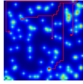
(a)

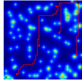
(b)

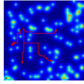
(c)

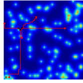
(d)

Figure 1: Different behaviors under different goal states and goal rewards: Figure 1a and Figure 1b share the same goal state, but the goal reward of Figure 1b is larger than Figure 1a.Figure 1c and Figure 1d share the same goal state, but the goal reward of Figure 1d is larger than Figure 1c. Five trajectories are plotted in each figure, where red dots denote the starting point and black dots denote the ending point.

In many IRL applications, we observe that a demonstrator usually has an inherent reward for each state, materialized as the innate state preferences of a human, the hardware-dependent cost function of a robot, the default structure of an environment, etc. For a given task, the demonstrators are usually reluctant to drastically change the inherent reward function to complete the task; instead, they alter the innate reward function minimally to generate a task-specific reward function and plan the motion. For example, in path planning, the C-space of a mobile robot at home rarely changes, and the robot’s motion depends on the goal state; in human motion analysis, the costs of different poses are mostly invariant, while the actual motion depends on the desired directions.

Based on this observation, we propose a meta inverse reinforcement learning algorithm by maximizing the shared rewards among all tasks. We model the reward function for each task as a probabilistic distribution conditioned on an inherent baseline function, and estimate the most likely reward function in the distribution that explains the observed task-specific demonstrations.

We review existing IRL and meta-learning algorithms in Section II, and then introduce the proposed method in Section III. We show a simulated experiments for evaluation and a real-world experiment for application in Section IV, with conclusions in Section V.

II Related Works

The idea of inverse optimal control is proposed by Kalman [5], white the inverse reinforcement learning problem is firstly formulated in [1], where the agent observes the states resulting from an assumingly optimal policy, and tries to learn a reward function that makes the policy better than all alternatives. Since the goal can be achieved by multiple reward functions, this paper tries to find one that maximizes the difference between the observed policy and the second best policy. This idea is extended by [6], in the name of max-margin learning for inverse optimal control. Another extension is proposed in [3], where the purpose is not to recover the real reward function, but to find a reward function that leads to a policy equivalent to the observed one, measured by the amount of rewards collected by following that policy.

Since a motion policy may be difficult to estimate from observations, a behavior-based method is proposed in [7], which models the distribution of behaviors as a maximum-entropy model on the amount of reward collected from each behavior. This model has many applications and extensions. For example, [8] considers a sequence of changing reward functions instead of a single reward function. [9] and [10] consider complex reward functions, instead of linear one, and use Gaussian process and neural networks, respectively, to model the reward function. [11] considers complex environments, instead of a well-observed Markov Decision Process, and combines partially observed Markov Decision Process with reward learning. [12] models the behaviors based on the local optimality of a behavior, instead of the summation of rewards. [13] uses a multi-layer neural network to represent nonlinear reward functions.

Another method is proposed in [14], which models the probability of a behavior as the product of each state-action’s probability, and learns the reward function via maximum a posteriori estimation. However, due to the complex relation between the reward function and the behavior distribution, the author uses computationally expensive Monte-Carlo methods to sample the distribution. This work is extended by [15], which uses sub-gradient methods to simplify the problem. Another extensions is shown in [16], which tries to find a reward function that matches the observed behavior. For motions involving multiple tasks and varying reward functions, methods are developed in [17] and [18], which try to learn multiple reward functions.

Most of these methods need to solve a reinforcement learning problem in each step of reward learning, thus practical large-scale application is computationally infeasible. Several methods are applicable to large-scale applications. The method in [1] uses a linear approximation of the value function, but it requires a set of manually defined basis functions. The methods in [10, 19] update the reward function parameter by minimizing the relative entropy between the observed trajectories and a set of sampled trajectories based on the reward function, but they require a set of manually segmented trajectories of human motion, where the choice of trajectory length will affect the result. Besides, these methods solve large-scale problems by approximating the Bellman Optimality Equation, thus the learned reward function and Q function are only approximately optimal. In our previous work, we proposed an approximation method that guarantees the optimality of the learned functions as well as the scalability to large state space problems [20].

To learn a model from limited data, meta learning algorithms are developed. A survey of different work is given in [21], viewing meta-learner as a way to improve biases for base-learners. The method in [22] uses neural memory machine to do the meta learning. The method in [23] minimizes the representations. The method in [24] learns by gradient descent. The method [25] learns optimizers.

Meta learning algorithms are also applied to reinforcement learning problems. The method in [26] tunes meta parameters for reinforcement learning, learning rate for TD learning, action selection trade-off, and discount factor. The method in [27] uses one network to play multiple games. The method in [28] trains reinforcement learning with slower rl. The method in [29] learns a good initial parameter that reaches optimal parameters with limited gradient descent. Meta learning in inverse reinforcement learning focuses on imitation learning, like one-shot imitation learning[30].

III Meta Inverse Reinforcement Learning

III-A Meta Inverse Reinforcement Learning

We assume that an agent needs to handle multiple tasks in an environment, denoted by $\{\mathbb{T}_{i}|i=1,N_{\mathbb{T}}\}$, where $\mathbb{T}_{i}$ denotes the $i_{th}$ task and $N_{\mathbb{T}}$ denotes the number of tasks.

We describe a task $\mathbb{T}_{i}$ as a Markov Decision Process, consisting of the following variables:

• $S_{i}=\{s\}$, a set of states

• $A_{i}=\{a\}$, a set of actions

• $P_{i,ss^{\prime}}^{a}$, a state transition function that defines the probability that state $s$ becomes $s^{\prime}$ after action $a$.

• $R_{i}=\{r_{i}(s)\}$, a reward function that defines the immediate reward of state $s$.

• $\gamma_{i}$, a discount factor that ensures the convergence of the MDP over an infinite horizon.

For a task $\mathbb{T}_{i}$, the agent performs a set of demonstrations $\zeta_{i}=\{\zeta_{i,j}|j=1,\cdots,N_{\zeta_{i}}\}$, represented by $N_{\zeta_{i}}$ sequences of state-action pairs:

$$\zeta_{i,j}=\{(s^{t}_{i,j},a^{t}_{i,j})|t=0,\cdots,N_{\zeta_{i,j}}\},$$

where $N_{\zeta_{i,j}}$ denotes the length of the $j_{th}$ sequence $\zeta_{i,j}$. Given the observed sequences $\zeta=\{\zeta_{i}|i=1,\cdots,N_{\mathbb{T}}\}$ for the $N_{\mathbb{T}}$ tasks, inverse reinforcement learning algorithms try to recover a reward function $r_{i}(s)$ for each task.

Our key observation in multi-task IRL is that the demonstrator has an inherent reward function $r_{b}(s)$, generating a baseline reward for each state in all tasks. To complete the $i_{th}$ task, the agent generates a reward function $r_{i}(s)$ from a distribution $P(r_{i}|r_{b})$ conditioned on $r_{b}(s)$ to plan the motion. Therefore, the motion $\zeta_{i}$ is generated as:

$$P(\zeta_{i}|r_{i})P(r_{i}|r_{b})$$

For the $i_{th}$ task, we want to find the most likely $r_{i}(s)$ sampled from $P(r_{i}|r_{b})$ that explains the demonstration $\zeta_{i}$. Assuming all the tasks are independent from each other, the following joint distribution is formulated:

$$\prod_{i=1}^{N_{\mathbb{T}}}P(\zeta_{i}|r_{i})P(r_{i}|r_{b})$$

The reward functions can be found via maximum-likelihood estimation:

$$\min_{r_{b}(s),r_{1}(s),\cdots,r_{\mathbb{T}}(s)\in\mathbb{F}}\sum_{i=1}^{N_{\mathbb{T}}}\underbrace{L_{i}(\zeta_{i},r_{i}(s))}_{\text{IRL loss}}+\underbrace{L(r_{i}(s),r_{b}(s))}_{\text{reward sharing loss}}$$ (1)

where $\mathbb{F}$ denotes a function space, $L_{i}(\zeta_{i},r_{i}(s))$ is the negative loglikelihood of $P(\zeta_{i}|r_{i})$, and $L(r_{i}(s),r_{b}(s))$ is the negative loglikelihood $P(r_{i}|r_{b})$.

III-B Loss for Inverse Reinforcement Learning

While many solutions exist for the inverse reinforcement learning problem, we adopt the solution based on function approximation developed in our earlier work [20] to handle the practical high-dimensional state spaces.

The core idea of the method is to approximate the Bellman Optimality Equation [2] with a function approximation framework. The Bellman Optimality Equation is given as:

$$V^{*}_{i}(s)=\max_{a\in A}\sum_{s^{\prime}|s,a}P_{i,ss^{\prime}}^{a}[r_{i}(s^{\prime})+\gamma*V_{i}^{*}(s^{\prime})],$$ (2)

$$Q^{*}_{i}(s,a)=\sum_{s^{\prime}|s,a}P_{i,ss^{\prime}}^{a}[r_{i}(s^{\prime})+\gamma*\max_{a^{\prime}\in A}Q_{i}^{*}(s^{\prime},a^{\prime})].$$ (3)

It is computationally prohibitive to solve in high-dimensional state spaces.

But with a parameterized VR function, we describe the summation of the reward function and the discounted optimal value function as:

$$f_{i}(s,\theta_{i})=r_{i}(s)+\gamma*V_{i}^{*}(s),$$ (4)

where $\theta_{i}$ denotes the parameter of VR function. The function value of a state is named as VR value.

Substituting Equation (4) into Bellman Optimality Equation, the optimal Q function is given as:

$$Q_{i}^{*}(s,a)=\sum_{s^{\prime}|s,a}P_{i,ss^{\prime}}^{a}f_{i}(s^{\prime},\theta_{i}),$$ (5)

the optimal value function is given as:

$$V_{i}^{*}(s)=\max_{a\in A}\sum_{s^{\prime}|s,a}P_{i,ss^{\prime}}^{a}f_{i}(s^{\prime},\theta_{i}),$$ (6)

and the reward function can be computed as:

$$r_{i}(s)=f_{i}(s,\theta_{i})-\gamma*\max_{a\in A}\sum_{s^{\prime}|s,a}P_{i,ss^{\prime}}^{a}f_{i}(s^{\prime},\theta_{i}).$$ (7)

This framework avoids solving the Bellman Optimality Equation. Besides, this formulation can be generalized to other extensions of Bellman Optimality Equation by replacing the $max$ operator with other types of Bellman backup operators. For example, $V^{*}(s)=\log\sum_{a\in A}\exp Q^{*}(s,a)$ is used in the maximum-entropy method[7]; $V^{*}(s)=\frac{1}{k}\log\sum_{a\in A}\exp k*Q^{*}(s,a)$ is used in Bellman Gradient Iteration [31].

To apply this framework to IRL problems, this work chooses a motion model $p(a|s)$ based on the optimal Q function $Q_{i}^{*}(s,a)$ [14]:

$$P(a|s)=\frac{\exp{b*Q_{i}^{*}(s,a)}}{\sum_{\tilde{a}\in A}\exp{b*Q_{i}^{*}(s,\tilde{a})}},$$ (8)

where $b$ is a parameter controlling the degree of confidence in the agent’s ability to choose actions based on Q values. Other models can also be used, like $p(a|s)=\exp(Q(s,a)-V(s))$ in [7].

Assuming the approximation function is a neural network, the parameter $\theta_{i}=\{w,b\}$-weights and biases, the negative log-likelihood of $P(\zeta_{i}|\theta_{i})$ is given by:

$$L_{i}(\theta_{i})=-\sum_{(s,a)\in\zeta_{i}}(b*Q_{i}^{*}(s,a)-\log{\sum_{\hat{a}\in A}\exp{b*Q_{i}^{*}(s,\hat{a}))}},$$ (9)

where the optimal Q function is given by Equation (5). After estimating the parameter $\theta_{i}$, the value function and reward function can be computed with Equation (4), (6), and (7).

III-C Loss for Reward Sharing

Since the demonstrator makes minimal changes to adapt the inherent reward function $r_{b}(s)$ into task-specific one $r_{i}(s)$, we model the distribution as:

$$P(r_{i}(s)|r_{b}(s))\propto\exp{(\mathbb{D}(r_{i}(s),r_{b}(s))))}$$

where $\mathbb{D}(r_{i}(s),r_{b}(s)))$ measures the difference between $r_{i}(s)$ and $r_{b}(s)$. Thus the loss function for reward sharing is given as:

$$L(r_{i}(s),r_{b}(s))=\log{Z}-\mathbb{D}(r_{i}(s),r_{b}(s)))$$

where $\log{Z}$ is the partition function and remains the same for all $r_{i}(s)$.

We test several functions as $\mathbb{D}(r_{i}(s),r_{b}(s)))$. The first choice is L2 loss, where

$$D(r_{i}(s),r_{b}(s))=||\{r_{i}(s)-r_{b}(s)\}||$$

where $\{r_{i}(s)-r_{b}(s)\}$ denotes the set of differences, evaluated on the full state space or only the visited states.

The second choice is Huber loss with $\delta=1$, a differentiable approximation of the L1 loss popular in sparse models:

$$L_{\delta}(a)={\begin{cases}{\frac{1}{2}}{a^{2}}&{\text{for }}|a|\leq\delta,\\ \delta(|a|-{\frac{1}{2}}\delta),&{\text{otherwise,}}\end{cases}},$$

and

$$D(r_{i}(s),r_{b}(s))=\sum_{s}L_{1}(r_{i}(s)-r_{b}(s)).$$

The third choice is standard deviation:

$$D(r_{i}(s),r_{b}(s))=stdev(\{r_{i}(s)-r_{b}(s)\})$$

The fourth choice is information entropy, after converting $\{r_{i}(s)-r_{b}(s)\}$ into a probabilistic distribution with sofmax function:

$$D(r_{i}(s),r_{b}(s))=entropy(softmax(\{r_{i}(s)-r_{b}(s)\}))$$

With the loss function for IRL and reward sharing, the reward functions can be learned via gradient method. The algorithm is shown in Algorithm 1.

Algorithm 1 Meta IRL

1:  Data: $\zeta,S,A,P,\gamma,b,\alpha$

2:  Result: reward value $R[S]$

3:  create variable $\theta_{b}=\{W,b\}$ for a neural network

4:  create variable $\theta_{i}=\{W,b\},i=1,\cdots,\mathbb{T}$ for each task

5:  initialize $\theta_{b},\theta_{i}=\{W,b\},i=1,\cdots,\mathbb{T}$

6:  while Not converging do

7:     update $\theta_{b},\theta_{i}=\{W,b\},i=1,\cdots,\mathbb{T}$ based on optimization (1)

8:  end while

9:  compute and return all $R_{i}[S]$

IV Experiments

IV-A Path Planning

We consider a path planning problem on an uneven terrain, where an agent can observe the whole terrain to find the optimal paths from random starting points to arbitrary goal points, but a mobile robot can only observe the agent’s demonstrations to learn how to plan paths. Given a starting point and a goal point, an optimal path depends solely on the costs to move across the terrain. To learn the costs, we formulate a Markov Decision Process for each goal point, where a state denotes a small region of the terrain and an action denotes a possible movement. The reward of a state equals to the negative of the cost to move across the corresponding region, while the goal state has an additional reward to attract movements.

In this work, we create a discretized terrain with several hills, where each hill is defined as a peak of cost distribution and the costs around each hill decay exponentially, and the true cost of a region is the summation of the costs from all hills. Ten worlds are randomly generated, and in each world, ten tasks are generated, each with a different goal state. For each task, the agent demonstrates ten trajectories, where the length of a trajectory depends on how many steps to reach the goal state.

We evaluate the proposed method with different reward sharing loss functions under different number of tasks and different number of trajectories. The evaluated loss functions include no reward sharing, reward sharing with standard deviation, information entropy, L2 loss, and huber loss. The number of tasks ranges from 1 to 16, and for each task, the number of trajectories ranges from 1 to 10. The learning rate is 0.01, with Adam optimizer. The accuracy of a reward is computed as the correlation coefficient between the learned reward function and the ground truth one. The results are shown in Figure 2.

The result shows that the meta learning step can significantly improve the accuracy of reward learning, among which the huber loss function leads to the best performance in average. L2 loss and standard deviation have similar performance, not surprisingly. However, the information entropy has a really bad performance.

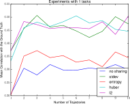
(a) 1 task

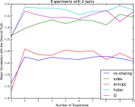
(b) 2 tasks

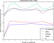
(c) 3 tasks

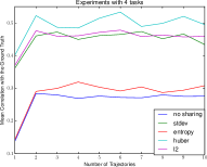
(d) 4 tasks

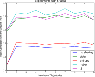
(e) 5 tasks

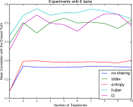
(f) 6 tasks

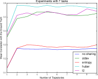
(g) 7 tasks

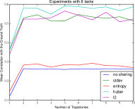
(h) 8 tasks

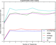
(i) 9 tasks

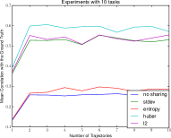
(j) 10 tasks

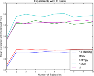
(k) 11 tasks

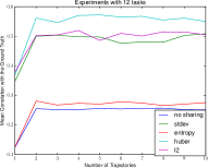
(l) 12 tasks

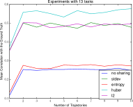
(m) 13 tasks

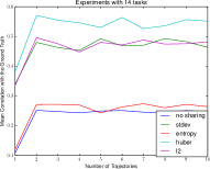
(n) 14 tasks

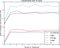
(o) 15 tasks

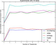
(p) 16 tasks

Figure 2: The result with five reward sharing loss functions on 16 tasks with at most 10 demonstrations for each task in 10 environment.

IV-B Motion Analysis

During rehabilitation, a patient with spinal cord injuries sits on a box, with a flat plate force sensor mounted on box to capture the center-of-pressure (COP) of the patient during movement. Each experiment is composed of two sessions, one without transcutaneous stimulation and one with stimulation. The electrodes configuration and stimulation signal pattern are manually selected by the clinician [32].

In each session, the physician gives eight (or four) directions for the patient to follow, including left, forward left, forward, forward right, right, right backward, backward, backward left, and the patient moves continuously to follow the instruction. The physician observes the patient’s behaviors and decides the moment to change the instruction.

Six experiments are done, each with two sessions. The COP trajectories in Figure 3 denote the case with four directional instructions; Figure 4, 5, 6, 7, and 8 denote the sessions with eight directional instructions.

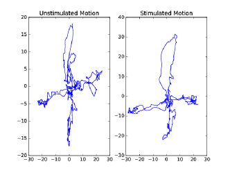
Figure 3: Patient 1 under four directional instructions: ”unstimulated motion” means that the patient moves without transcutaneous stimulations, while ”stimulated motion” represents the motion under stimulations.

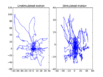
Figure 4: Patient 2 under eight directional instructions: ”unstimulated motion” means that the patient moves without transcutaneous stimulations, while ”stimulated motion” represents the motion under stimulations.

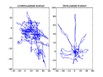
Figure 5: Patient 3 under eight directional instructions: ”unstimulated motion” means that the patient moves without transcutaneous stimulations, while ”stimulated motion” represents the motion under stimulations.

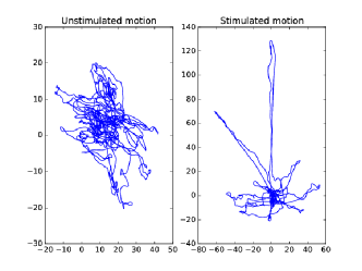
Figure 6: Patient 4 under eight directional instructions: ”unstimulated motion” means that the patient moves without transcutaneous stimulations, while ”stimulated motion” represents the motion under stimulations.

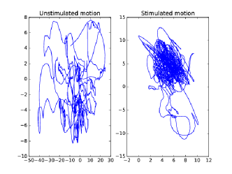
Figure 7: Patient 5 under eight directional instructions: ”unstimulated motion” means that the patient moves without transcutaneous stimulations, while ”stimulated motion” represents the motion under stimulations.

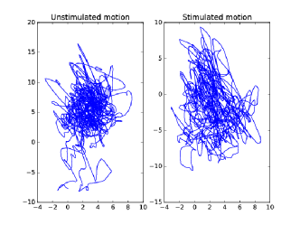
Figure 8: Patient 6 under eight directional instructions: ”unstimulated motion” means that the patient moves without transcutaneous stimulations, while ”stimulated motion” represents the motion under stimulations.

The COP sensory data from each session is discretized on a $100\times 100$ grid, which is fine enough to capture the patient’s small movements. The problem is formulated into a MDP, where each state captures the patient’s discretized location and velocity, and the set of actions changes the velocity into eight possible directions. The velocity is represented with a two-dimensional vector showing eight possible velocity directions. Thus the problem has 80000 states and 8 actions, and each action is assumed to lead to a deterministic state.

TABLE I: Evaluation of the learned rewards: ”forward” etc. denote the instructed direction; item name”1u” denotes the patient id ”1”, with ”u” denoting unstimulated session and ”s” denoting stimulated sessions. The table shows the correlation coefficient between the ideal reward and the recovered reward.

	forward	backward	left	right	top left	top right	bottom left	bottom right	origin
1u	0.411741	0.257564	0.0691989	-0.210216					0.49016
1s	0.200355	0.486723	0.129839	0.436533					0.207188
2u	0.161595	-0.17814	0.153376	-0.16767	0.162906	0.105993	-0.0211192	-0.220457	0.156034
2s	-0.0310265	-0.0803484	0.0474505	-0.00146299	0.0442916	0.0874981	0.00668849	0.0742221	0.0726437
3u	0.362801	-0.2995	0.245916	-0.178778	0.386421	0.0148849	-0.00335653	-0.385605	0.0507719
3s	-0.265834	0.146516	0.379665	-0.272437	0.138805	-0.2683	0.212331	0.00301386	-0.182916
4u	0.301472	-0.281474	0.377787	-0.320403	0.410212	-0.119599	0.136309	-0.306677	0.171433
4s	-0.104719	0.0930068	0.327783	-0.229091	0.175432	-0.161819	0.323862	-0.0521654	-0.202197
5u	0.360293	-0.311692	-0.253715	0.260426	0.0863029	0.495134	-0.38137	-0.140836	-0.160687
5s	-0.212823	0.0414435	0.0908994	-0.124174	0.00414109	-0.107462	0.122018	0.0453461	0.145686
6u	-0.0416432	0.0570847	0.210028	-0.104113	0.0363181	-0.0672399	0.0704143	-0.00392284	0.190253
6s	-0.157148	0.178879	0.0880393	-0.0718817	-0.102579	-0.298918	0.307328	0.171319	0.359168

To learn the reward function from the observed trajectories based on the formulated MDP, we use the coordinate and velocity direction of each grid as the feature, and learn the reward function parameter from each set of data after segmentation based on peak detection on distances from the origin. The function approximator is a neural network with three hidden layers and $[100,50,25]$ nodes. The huber loss function is used in reward sharing, and the result is show in Table I.

It shows that the patient’s ability to following instructions vary among different directions, and the values will assist physicians to design the stimulating signals.

V Conclusions

This work proposes a solution to learn an accurate reward function for each task with limited demonstrations but from the same demonstrator, by maximizing the shared rewards among different tasks. We proposed several loss functions to maximize the shared reward, and compared their accuracies in a simulated environment. It shows that huber loss has the best performance.

In future work, we will apply the proposed method to imitation learning.

References

- [1] A. Y. Ng and S. Russell, “Algorithms for inverse reinforcement learning,” in in Proc. 17th International Conf. on Machine Learning, 2000.
- [2] R. S. Sutton and A. G. Barto, Reinforcement learning: An introduction. MIT press Cambridge, 1998, vol. 1, no. 1.
- [3] P. Abbeel and A. Y. Ng, “Apprenticeship learning via inverse reinforcement learning,” in Proceedings of the twenty-first international conference on Machine learning. ACM, 2004, p. 1.
- [4] B. Najafi, K. Aminian, A. Paraschiv-Ionescu, F. Loew, C. J. Bula, and P. Robert, “Ambulatory system for human motion analysis using a kinematic sensor: monitoring of daily physical activity in the elderly,” IEEE Transactions on biomedical Engineering, vol. 50, no. 6, pp. 711–723, 2003.
- [5] R. Kalman and M. M. C. B. D. R. I. for Advanced Studies. Center for Control Theory, When is a Linear Control System Optimal?., ser. RIAS technical report. Martin Marietta Corporation, Research Institute for Advanced Studies, Center for Control Theory, 1963.
- [6] N. D. Ratliff, J. A. Bagnell, and M. A. Zinkevich, “Maximum margin planning,” in Proceedings of the 23rd international conference on Machine learning. ACM, 2006, pp. 729–736.
- [7] B. D. Ziebart, A. Maas, J. A. Bagnell, and A. K. Dey, “Maximum entropy inverse reinforcement learning,” in Proc. AAAI, 2008, pp. 1433–1438.
- [8] Q. P. Nguyen, B. K. H. Low, and P. Jaillet, “Inverse reinforcement learning with locally consistent reward functions,” in Advances in Neural Information Processing Systems, 2015, pp. 1747–1755.
- [9] S. Levine, Z. Popovic, and V. Koltun, “Nonlinear inverse reinforcement learning with gaussian processes,” in Advances in Neural Information Processing Systems 24, J. Shawe-Taylor, R. S. Zemel, P. L. Bartlett, F. Pereira, and K. Q. Weinberger, Eds. Curran Associates, Inc., 2011, pp. 19–27.
- [10] C. Finn, S. Levine, and P. Abbeel, “Guided cost learning: Deep inverse optimal control via policy optimization,” arXiv preprint arXiv:1603.00448, 2016.
- [11] J. Choi and K.-E. Kim, “Inverse reinforcement learning in partially observable environments,” Journal of Machine Learning Research, vol. 12, no. Mar, pp. 691–730, 2011.
- [12] S. Levine and V. Koltun, “Continuous inverse optimal control with locally optimal examples,” arXiv preprint arXiv:1206.4617, 2012.
- [13] M. Wulfmeier, P. Ondruska, and I. Posner, “Deep inverse reinforcement learning,” arXiv preprint arXiv:1507.04888, 2015.
- [14] D. Ramachandran and E. Amir, “Bayesian inverse reinforcement learning,” in Proceedings of the 20th International Joint Conference on Artifical Intelligence, ser. IJCAI’07. San Francisco, CA, USA: Morgan Kaufmann Publishers Inc., 2007, pp. 2586–2591.
- [15] G. Neu and C. Szepesvári, “Apprenticeship learning using inverse reinforcement learning and gradient methods,” arXiv preprint arXiv:1206.5264, 2012.
- [16] K. Mombaur, A. Truong, and J.-P. Laumond, “From human to humanoid locomotion—an inverse optimal control approach,” Autonomous robots, vol. 28, no. 3, pp. 369–383, 2010.
- [17] C. Dimitrakakis and C. A. Rothkopf, “Bayesian multitask inverse reinforcement learning,” in European Workshop on Reinforcement Learning. Springer, 2011, pp. 273–284.
- [18] J. Choi and K.-E. Kim, “Nonparametric bayesian inverse reinforcement learning for multiple reward functions,” in Advances in Neural Information Processing Systems, 2012, pp. 305–313.
- [19] A. Boularias, J. Kober, and J. R. Peters, “Relative entropy inverse reinforcement learning,” in International Conference on Artificial Intelligence and Statistics, 2011, pp. 182–189.
- [20] K. Li and J. W. Burdick, “Large-scale inverse reinforcement learning via function approximation for clinical motion analysis,” arXiv preprint arXiv:1707.09394, 2017.
- [21] R. Vilalta and Y. Drissi, “A perspective view and survey of meta-learning,” Artificial Intelligence Review, vol. 18, no. 2, pp. 77–95, 2002.
- [22] A. Santoro, S. Bartunov, M. Botvinick, D. Wierstra, and T. Lillicrap, “Meta-learning with memory-augmented neural networks,” in International conference on machine learning, 2016, pp. 1842–1850.
- [23] B. Hariharan and R. Girshick, “Low-shot visual recognition by shrinking and hallucinating features,” arXiv preprint arXiv:1606.02819, 2016.
- [24] M. Andrychowicz, M. Denil, S. Gomez, M. W. Hoffman, D. Pfau, T. Schaul, and N. de Freitas, “Learning to learn by gradient descent by gradient descent,” in Advances in Neural Information Processing Systems, 2016, pp. 3981–3989.
- [25] D. Ha, A. Dai, and Q. V. Le, “Hypernetworks,” arXiv preprint arXiv:1609.09106, 2016.
- [26] N. Schweighofer and K. Doya, “Meta-learning in reinforcement learning,” Neural Networks, vol. 16, no. 1, pp. 5–9, 2003.
- [27] E. Parisotto, J. L. Ba, and R. Salakhutdinov, “Actor-mimic: Deep multitask and transfer reinforcement learning,” arXiv preprint arXiv:1511.06342, 2015.
- [28] Y. Duan, J. Schulman, X. Chen, P. L. Bartlett, I. Sutskever, and P. Abbeel, “Rl2: Fast reinforcement learning via slow reinforcement learning,” arXiv preprint arXiv:1611.02779, 2016.
- [29] C. Finn, P. Abbeel, and S. Levine, “Model-agnostic meta-learning for fast adaptation of deep networks,” arXiv preprint arXiv:1703.03400, 2017.
- [30] Y. Duan, M. Andrychowicz, B. Stadie, J. Ho, J. Schneider, I. Sutskever, P. Abbeel, and W. Zaremba, “One-shot imitation learning,” arXiv preprint arXiv:1703.07326, 2017.
- [31] K. Li and J. W. Burdick, “Bellman Gradient Iteration for Inverse Reinforcement Learning,” ArXiv e-prints, Jul. 2017.
- [32] S. Harkema, Y. Gerasimenko, J. Hodes, J. Burdick, C. Angeli, Y. Chen, C. Ferreira, A. Willhite, E. Rejc, R. G. Grossman et al., “Effect of epidural stimulation of the lumbosacral spinal cord on voluntary movement, standing, and assisted stepping after motor complete paraplegia: a case study,” The Lancet, vol. 377, no. 9781, pp. 1938–1947, 2011.