MoNoise: Modeling Noise Using a Modular Normalization System.

Abstract

We propose MoNoise: a normalization model focused on generalizability and efficiency, it aims at being easily reusable and adaptable. Normalization is the task of translating texts from a non-canonical domain to a more canonical domain, in our case: from social media data to standard language. Our proposed model is based on a modular candidate generation in which each module is responsible for a different type of normalization action. The most important generation modules are a spelling correction system and a word embeddings module. Depending on the definition of the normalization task, a static lookup list can be crucial for performance. We train a random forest classifier to rank the candidates, which generalizes well to all different types of normalization actions. Most features for the ranking originate from the generation modules; besides these features, N-gram features prove to be an important source of information. We show that MoNoise beats the state-of-the-art on different normalization benchmarks for English and Dutch, which all define the task of normalization slightly different.

1 Introduction

The spontaneous and diverse nature of language use on social media leads to many problems for existing natural language processing models. Most existing models are developed with a focus on more canonical language. These models do not cope with the disfluencies and unknown phenomena occurring in social media data. This is also known as the problem of domain adaptation: in which we try to adapt a model trained on a source domain to another target domain. Solutions for this problem can be broadly divided in two strategies: adapting the model to the target domain, or adapting the data to the source domain (?).

Domain adaptation by adapting the model to the target domain can be done in different ways. The most straightforward method is to train the model on annotated data from the target domain. Newly annotated data can be obtained by hiring human annotators. However, it is cheaper to annotate data automatically using an existing model. This is called self-training, or up-training if the data is annotated by an external model. The effect of adding this newly annotated data depends on the nature of the new data compared to the data of the target and source domain. The added data should be annotated with a high accuracy, so it can not be too distant from the source domain. However, it should add some information inherent to the target domain. There is ample previous work in this direction in which different strategies of up-training are used (?, ?, ?).

The other strategy for domain adaptation is to convert the data to the source domain; this is the strategy explored in this work. This task is often referred to as normalization, because we aim to convert data from the target domain to the more ’normal’ source domain, for which a model is already available. The main advantage of this approach is that we only need one normalization model, which we can use as preprocessing step for multiple natural language processing systems.

Normalization is a subjective task; the goal is to convert to ‘normal’ language. At the same time, we must preserve the meaning of the original utterance. This task comprises the correction of unintentional anomalies (spell correction) as well as intentional anomalies (domain specific language phenomena). Annotator disagreement can thus have two sources, the decision whether a word should be normalized, and the choice of the correct normalization candidate. We discuss these problems in more depth in Section 3.1. In the rest of this paper we will use the term ‘anomaly’ for words in need of normalization according to the annotators.

Ima regret bein up this late 2mr
I’m going to regret being up this late tomorrow

Example 1 shows that the normalization task comprises of different types of transformations. Replacements like ‘bein’ $\mapsto$ ‘being’ are quite similar on the surface, whereas ‘tmr’ $\mapsto$ tomorrow shows that we need more than edit distances on the character level. This example includes a 1-N replacement (Ima $\mapsto$ ‘I’m going to’, meaning that a single token is mapped to multiple tokens. Not all the annotated corpora we use include annotation for these cases (see Section 3.1). 1-N replacements show a strong Zipfian distribution in the corpora that include them in the annotation, because of the expansion of phrasal abbreviations like ‘lol’ and ‘idk’ which are very common. Some of the corpora also include N-1 replacements, meaning the merging of two consecutive words; however, this is a very rare phenomenon.

Because the normalization problem comprises of a variety of different normalization actions required for different types of anomalies, we propose to tackle this problem in a modular way. Different modules can then be designed for different types of anomalies. Our most important modules are: a spell correction module, a word embeddings module, and a static lookup list generated from the training data. We use features from the generation modules as well as additional features in a random forest classifier, which decides which candidate is the correct normalization. We experiment with a variety of additional features, of which the N-gram features are by far the best predictor.

The rest of this paper is structured as follows: We first discuss related work (Section 2), after which we shortly describe the used data (Section 3). Next follows the methodology section (4) and the evaluation section (5), which are both splitted by the two different parts of our system; candidate generation and candidate ranking. Finally, we conclude in Section 6.

2 Related Work

The first attempts at normalizing user generated content were focused on SMS data; ? annotated a dataset for this domain, and reported the first results. They use a Hidden Markov Model encoding based on characters and phonemic transcriptions to model the word variation in SMS data. The Viterbi algorithm is then used to find the most likely replacement for each position.

Later, focus shifted towards normalization for social media, more specifically: the Twitter domain. The first work on normalization for this domain was from ?. They released the LexNorm corpus, consisting of 549 Tweets annotated with their normalization on the word level. Annotation is restricted to word to word replacements, so words like ‘gonna’ are kept untouched. ? also reported the first results on this dataset. They train a support vector machine which predicts if a word needs normalization based on dependency tree context; the length of the arcs and the head words are used as predictors. After this, they generate candidates using a combination of lexical and phonetic edit distances. Candidates are ranked using a combination of dictionary lookup, word similarity and N-gram probabilities. Note that on this corpus, gold error detection is usually assumed, accuracy is reported on only the words that need normalization.

Over the years, many different approaches have been benchmarked on this dataset;  ? experiment with character based machine translation. ? use random walks in a bipartite graph based on words and their contexts to generate normalization candidates, which they rank using the Viterbi algorithm. A log-linear model was explored by ?, they use sequential Monte Carlo to approximate feature expectation, and rank them using a Viterbi-encoding. Whereas most previous work normalizes on the word level or character level,  ? attempt to normalize on the syllable level. They translate noisy words to sequences of syllables, which can then be normalized to canonical syllables, which can in turn be merged back to form normalization candidates.

To the best of our knowledge, ? reported the highest accuracy on the LexNorm dataset. They rerank the results of six different normalization systems, including machine translation systems, a character sequence labeling model and a spell checker. Each normalization system suggests one candidate. A Viterbi decoding based on the candidates and their possible POS tags is then used to rank the candidates. This joint approach is beneficial for both tasks.

More recently, the 2015 Workshop on Noisy User-generated Text hosted a shared task on lexical normalization (?). They defined the task slightly different compared to the annotation of the LexNorm corpus. Annotation included 1-N and N-1 replacements. N-1 replacements indicate merging, which occurs very rarely. For the shared task, gold error detection was not assumed, and was part of the task. A total of 10 teams participated in this shared task, using a wide variety of approaches. For generation of candidates the most commonly used methods include: character N-grams, edit-distances and lookup lists. Ranking was most often done by conditional random fields, recurrent neural networks or the Viterbi algorithm.

The best results on this new benchmark were obtained by ?. This model generates candidates based on a lookup list, all possible splits and a novel similarity index: the Jaccard index based on character N-grams and character skip-grams. This novel similarity index is used to find the most similar candidates from a dictionary compiled from the golden training data.  ? also tests if it is beneficial to find similar candidates in the Aspell dictionary, but concludes that this leads to over-normalization. The candidates are ranked using a random forest classifier, using a variety of features: frequency counts in training data, a novel similarity index and POS tagging confidence.

Most of the previous work has been on the English language, although there has been some work on other languages. We will consider normalization for Dutch to test if our proposed model can be effective for other languages. There has already been some previous work on normalization for the Dutch language.  ? annotated a normalization corpus consisting of three user generated domains. They experiment on this data with machine translation on the word and character level, and report a 20% gain in BLEU score, including tokenization corrections. Building on this work,  ? built a multi-modular model, in which each module accounts for different normalization problems, including: machine translation modules, a lookup list and a spell checker. They also report improved results for extrinsic evaluations on three tasks: POS tagging, lemmatization and named entity recognition.

Our proposed system is the most similar to ?; however, there are many differences. The main differences are that we use word-embeddings for generation and include N-grams features for ranking, which can easily be obtained from raw text. This makes the system more general and easier adaptable to new data. The system from ? is more focused towards the given corpus, and might have more difficulties on data from another time span or another social media domain.

3 Data

The data we use can be divided in two parts: data annotated for normalization, and other data.

3.1 Normalization Corpora

The normalization task can be seen as a rather subjective task; the annotators are asked to convert noisy texts to ‘normal’ language. The annotation guidelines are usually quite limited (?, ?), leaving space for interpretation; which might lead to inconsistent annotation. ? report a Fleiss’ $\kappa$ of 0.891 on the detection of words in the need of normalization. They also shared the annotation efforts of each annotator, we used this data to calculate the pairwise human performance on the choice of the correct normalization candidate. This revealed that the annotators agree on the choice of the normalized word in 98.73% of the cases. Note that this percentage is calculated assuming gold error detection. ? report a Cohen’s $\kappa$ of 0.5854 on the complete normalization task, a lot lower compared to ?. Hence, we can conclude that the inter-annotator agreement is quite dependent on the annotation guidelines. After the decision whether to normalize, annotator agreement is quite high on the choice of the correct candidate.

Corpus	Source	Words	Lang.	Caps	Multiword	%normalized
LexNorm1.2	?	10,564	en	no	no	11.6
LiLiu	?	40,560	en	some	no	10.5
LexNorm2015	?	44,385	en	no	yes	8.9
GhentNorm	?	12,901	nl	yes	yes	4.8

Table 1: Comparison of the different corpora used in this work.

The main differences between the different normalization corpora are shown in Table 1. Note that we use the LexNorm1.2 corpus, which contains some annotation improvements compared to the original LexNorm corpus. The GhentNorm corpus is the only corpus fully annotated with capitals, even though the capital-use is not corrected; it is preserved from the original utterance (?). The multiword column represents whether 1-N and N-1 replacements are included in the annotation guidelines; the corpora which do include this, also include expansions of commonly used phrasal abbreviations as ‘lol’ and ‘lmao’, and N-1 replacements are extremely rare. There is some difference in the percentage of tokens that are normalized, probably due to differences in filtering and annotation.

To give a better idea of the nature of the data and annotation, we will discuss some example sentences below.

lol or it could b sumthn else …
lol or it could be something else …

Example 3.1 comes from the LiLiu corpus, this example contains two replacements. The replacements are subsequent words, which is not uncommon; this leads to problems for using context directly. The replacement ‘b’ $\mapsto$ ‘be’ is grammatically close, whereas the replacement of ‘sumthn’ $\mapsto$ ‘something’ is more distant, and would be harder to solve with traditional spelling correction algorithms.

$<$USERNAME$>$ i aint messin with no1s wifey yo lol
$<$USERNAME$>$ i ain’t messing with no one’s wifey you laughing out loud

Example 3.1 is taken from the LexNorm2015 corpus. This annotation also include 1-N replacements; ‘no1s’ and ‘lol’ are expanded. the word ‘no1s’ is not only splitted, but also contains a substitution of of a number to it’s written form; two actions are necessary. In contrast to the previous example, here the token ‘lol’ is expanded; this is a matter of differences in annotation guidelines. The annotator decided to leave the word ‘wifey’ as is, whereas it could have been normalized to wife, this reflects the suggested conservativity described in the annotation guidelines (?).

$<$USERNAME$>$ nee ! :-D kzal no es vriendelijk doen lol
$<$USERNAME$>$ nee ! :-D ik zal nog eens vriendelijk doen laughing out loud

Example 3.1 comes from the GhentNorm corpus. The word ‘ik’ (I) is often abbreviated and merged with a verb in Dutch Tweets, leading to ‘kzal’ which is correctly splitted in the annotation to ‘ik zal’ (I will). ‘no’ is probably a typographical mistake, whereas ‘es’ is a shortening based on pronunciation. Similar to the LexNorm 2015 annotation, the phrasal abbreviation ‘lol’ is expanded.

3.2 Other Data

In addition to the training data, we also use some external data for our features. The Aspell dictionaries for Dutch and English are used as-is, including the expansions of words. Furthermore, we use two large raw text databases; one with social media data, and one from a more canonical domain.

For Dutch we used a collection of 1,545,871,819 unique Tweets collected between 2010 and 2016, they were collected based on a list of frequent Dutch tokens which are infrequent in other languages (?). For English we collected Tweets throughout 2016, based on the 100 most frequent words of the Oxford English Corpus , resulting in a dataset of 760,744,676 Tweets. We used some preprocessing to reduce the number of types, this leads to smaller models, and thus faster processing. We replace usernames and urls by $<$USERNAME$>$ and $<$URL$>$ respectively. As canonical raw data, we used Wikipedia dumps for both Dutch and English.

4 Method

The normalization task can be split into two sub-tasks:

• Candidate generation: generate possible normalization candidates based on the original word. This step is responsible for an uppperbound on recall; but care should also be taken to not generate too many candidates, since this could complicate the next sub-task.

• Candidate ranking: takes the generated candidate list from the previous sub-tasks as input, and tries to extract the correct candidate by ranking the candidates. In our setup we score all the candidates, so that a list of top-N candidates can be outputted.

Most previous work includes error detection as first step, and only explores the possibilities for normalization of words detected as anomaly. However, we postpone this decision by adding the original word as a candidate. This results in a more informed decision whether to normalize or not at ranking time. We will discuss the methods used for each of the two tasks separately in the next subsections.

4.1 Candidate Generation

We use different modules for candidate generation. Each module is focused on a different type of anomaly.

Original token

Because we do not include an error detection step, we need to include the original token in the candidate list. This module should provide the correct candidate in 90% of the cases in our corpora (Table 1).

Word embeddings

We use a word embeddings model trained on the social media domain using the Tweets described in Section 3.2. For each word we find the top 40 closest candidates in the vector space based on the cosine distance. We train a skip-gram model (?) for 5 iterations with a vector size of 400 and a window of 1.

Aspell

We use the Aspell spell checker to repair typographical errors. Aspell uses a combination of character edit distance, and a phonetic distance to generate similar looking and similar sounding words. We will use the ‘normal’ mode as default, but also experiment with the ‘bad-spellers’ mode, in which the algorithm allows for candidates with a larger distance to the original word, resulting in much bigger candidate lists. The effect of this setting is evaluated in more detail in Section 6.

Lookup-list

We generate a list of all replacement pairs occurring in the training data. When we encounter a word that occurs in this list, every normalization replacement occurring in the training data is added as candidate.

Word.*

As a result of space restrictions and input devices native to this domain, users often use abbreviated versions of words. To capture this phenomenon, we include a generation module that simply searches for all words in the Aspell dictionary which start with the character sequence of our original word. To avoid large candidate lists, we only activate this module for words longer than two characters.

Split

We generate word splits by splitting a word on every possible position and checking if both resulting words are canonical according to the Aspell dictionary. To avoid over-generation, this is only considered for input words larger than three characters.

To illustrate the effect of these generation modules, the top 3 candidates each of these modules generate for our example sentence are shown in Figure 1. This examples shows that the multiple modules complement each other rather well, they all handle different types of anomalies. The modules are evaluated separately in Section 5.1

Figure 1: The top 3 generated candidates for each of the generation modules.

4.2 Candidate Ranking

In this section we will first describe the features used for ranking, starting with the features which originate from the generation step. After this, we discuss the used classifier.

Original

A binary feature which indicates if a candidate is the original token.

Word embeddings

We use the cosine distance between the candidate and the original word in the vector space as a feature. Additionally, the rank of the candidate in the returned list is used as feature.

Aspell

Aspell returns a ranked list of correction candidates, we use the rank in this list as a feature. Additionally, we use the internal calculated distance between the candidate and the original word; this distance is based on lexical and phonetical edit distances. The internal edit distance can be obtained from the Aspell library using C++ function calls. Note that both of these features are only used for candidates generated by the Aspell module.

Lookup-list

In our training data we count the occurrences of every correction pair, this count is used as feature. Note that we also include counts for unchanged pairs in the training data; this strengthens the decision whether to keep the original word.

Word.*

We use a binary feature to indicate if a candidate is generated by this module.

N-grams

We use two different N-gram models from which we calculate the unigram probability, the bigram probability with the previous word, and the bigram probability with the next word. The first N-gram model is trained on the same Twitter data as the word embeddings, the second N-gram model is based on more canonical Wikipedia data (Section 3.2).

Dictionary lookup

A binary feature indicating if the candidate can be found in the Aspell dictionary.

Character order

We also include a binary feature indicating if the characters of the original token occur in the same order in the candidate.

Length

One feature indicates the length of the original word, and one for the length of the candidate.

ContainsAlpha

A binary feature indicating whether a token contains any alphabetical characters; in some annotation guidelines tokens which do not fit this restriction are kept untouched.

The task of picking the correct candidate can be seen as a binary classification task; a candidate is either the correct candidate or not. However, we can not use a binary classifier directly; because we need exactly one instance for the ‘correct’ class. Whereas the classifier might classify multiple or zero candidates per position as correct. Instead, we use the confidence of the classifier that a candidate belongs to the ‘correct’ class to rank the candidates. This has the additional advantage that it enables the system to output lists of top-N candidates for use in a pipeline.

We choose to use a random forest classifier (?) for the ranking of candidates. We choose this classifier because the problem of normalization can be divided in multiple normalization actions which behave differently feature wise, however in our setup they are all classified as the same class. A random forest classifier makes decisions based on multiple trees, which might take into account different features. Our hypothesis is that it builds different types of trees for different normalization actions. More concretely: if a candidate scores high on the Aspell feature (it has a low edit distance), this can be an indicator for a specific set of trees to give this candidate a high score. At the same time the model can still give very high scores to candidates with low values for the Aspell features. We use the implementation of Ranger (?), with the default parameters.

? showed that it might have a negative effect on performance to generate candidates that do not occur in the training data. For this reason we add an option to MoNoise to filter candidates based on a word list generated from the training data. Additionally we add an option to filter based on all words occurring in the training data complemented by the Aspell dictionary; these settings are evaluated in more detail in Section 6.

5 Evaluation

In this section, we will evaluate different aspects of the normalization systems. We evaluate on three benchmarks:

• LexNorm1.2: for testing on the LexNorm corpus, we use 2,000 Tweets from LiLiu (see Section 3.1) as training and the other 577 Tweets as development data.

• LexNorm2015: Consisting of 2,950 Tweets for training and 1,967 for testing. We use 950 Tweets from the training set as development data.

• GhentNorm: similar to previous work, we split the data in 60% training data, and both 20% development and test data.

For all these three datasets we evaluate the different modules of the candidate generation and the ranking. All evaluation in this section is done with all words lowercased, because it is in line with previous work and capitalization is not consistently annotated in the available datasets.

5.1 Candidate Generation

In this section we will first compare each of the modules in isolation. Next, we test how many unique correct normalization candidates each module contributes in an ablation experiment.

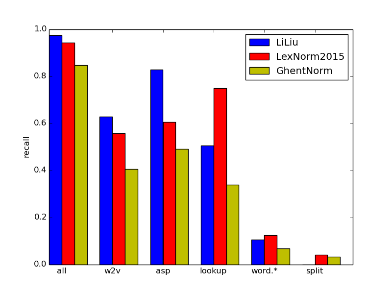
Figure 2: Recall of generation modules in isolation on the development corpora.

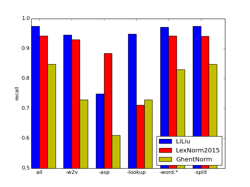
Figure 3: Ablation experiments for generation modules on the development corpora.

Module	Average candidates
w2v	34.13
Aspell	31.29
lookup	0.72
word.*	20.80
split	0.35

Table 2: The number of candidates generated by generation modules, averaged over the different development data sets.

The recall of the generation modules in isolation are plotted in Figure 2; the number of candidates each module generates on average over all datasets is shown in Table 2. The best performing modules in isolation are Aspell, word embeddings and the lookup module. The lookup module performs especially well on the LexNorm2015 corpus. This is due to a couple of correction pairs which occur very frequently (u, lol, idk, bro). The word.* module does not perform very well, it over-generates mainly on the GhentNorm corpus (average of 48 candidates). The split module can only generate correct candidates for corpora that contain 1-n word replacements. For these corpora, it generates a few correct candidates.

The performances of the ablation experiments are shown in Figure 3. Similar to the previous experiment, the most important modules are Aspell, word embeddings and the lookup module. However, the word embeddings contribute less unique candidates; presumably because it has overlap with both of the other modules. The differences between corpora are also similar to the previous experiment; the lookup list is also generating the most unique correct candidates for the LexNorm2015 corpus. Furthermore, this graph shows that word.* still generates some unique candidates, especially for the GhentNorm corpus. This suggests that this way of abbreviating is more common in Dutch.

5.2 Candidate Ranking

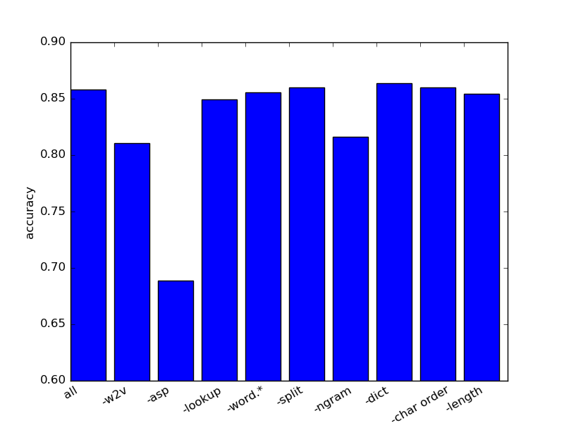
Figure 4: Accuracy only on words needing normalization when excluding feature groups on LiLiu development data.

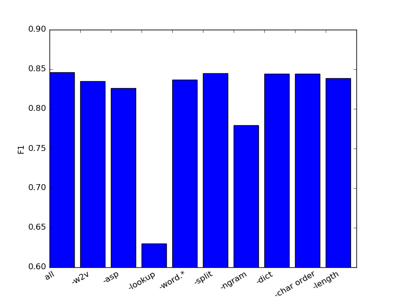
Figure 5: F1 scores when excluding feature groups on the LexNorm2015 development data.

Since candidate ranking is the final step, this section discusses the performance of the whole system. We compare the performance of our system with different benchmarks. First we consider the LexNorm corpus, for which most previous work assumed gold error detection. In order to be able to compare our results, we will assume the same. Additionally, we test our performance on LexNorm2015, which was used in the shared task of the 2015 workshop on Noisy User-generated Text (?). Here, error detection was included in the task, hence we will also use automatic error detection by including the original token as a candidate.

Figure 4 shows the importance of the different feature groups in the final model for the LiLiu development set. Aspell is the most important feature for this dataset. Except for the split module (which is not included in the annotation) all the features contribute to obtaining the highest score.

Figure 5 shows the F1 scores of the ablation experiments on the LexNorm2015 corpus. In this setup, the differences are smaller, except for the lookup module, which generates many unique phrasal abbreviations (lol, idk, smh). Perhaps surprisingly, word embeddings show a relatively small effect on the final performance. On both datasets, the N-gram module proves to be very valuable for this task.

#cands	LiLiu	LexNorm2015	GhentNorm
1	95.6	97.6	98.3
2	98.6	99.0	99.0
3	99.1	99.2	99.1
4	99.3	99.3	99.3
5	99.3	99.3	99.3
ceil.	99.6	99.4	99.8

Table 3: Recall achieved by the top-N candidates for our different development data sets. Note that this is over all words, also words not needing normalization.

To evaluate the performance of the ranking beyond the top-1 candidate, Table 3 shows the recall of the top-N candidates on the different datasets. This table shows that most of the mistakes the classifier makes are between the first and the second candidate. Manual inspection revealed that many of these are confusions with the original token; thus the decision whether normalization is necessary at all. Beyond the second candidate, there are only a few correct candidates to be found.

5.3 Additional Experiments

We test the effect of the size of the training data for the two largest datasets: LiLiu and LexNorm2015. The results are plotted in Figure 6. The higher F1 scores on the LexNorm2015 dataset are probably due to the common phrasal abbreviations. Based on these graphs, we can conclude that a reasonable performance can be achieved by using around 500 Tweets. However, the performance still improves at a training size of 2,000 Tweets.

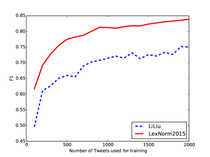
Figure 6: The effect of the size of training data on the LexNorm2015 and LiLiu dataset

As explained in Section 4 we included two options to tune the speed-performance ratio. Firstly, we can allow Aspell to generate larger lists of candidates by using the ‘bad-spellers’ mode. Secondly, we can filter the generated candidates, keeping only candidates which occur in the training data or in the Aspell dictionary. Table 4 shows the times the different combinations of parameters take to train and run on the LexNorm2015 dataset, as well as the performance and the number of candidates generated. The best performance is achieved by filtering based on words occurring in the training data combined with the Aspell dictionary and using the ‘normal’ mode. However, the ‘bad-spellers’ mode without filtering reaches on par performance and might be the preferable option, since it can be more robust to data from a different time period or different domain.

Aspell mode	Filter	Train time (m:s)	Words/sec.	F1	Upperbound	Avg. cands.
normal	-	4:56	82.4	83.4	99.5	74.2
normal	train+asp	2:35	121.2	84.2	99.2	38.7
normal	train	0:59	203.1	82.9	99.0	13.8
bad-spellers	-	28:31	23.4	84.1	99.5	306.8
bad-spellers	train+asp	19:19	31.4	84.0	99.3	208.7
bad-spellers	train	7:12	58.8	83.3	99.1	71.9

Table 4: Effect of using different Aspell modes on the LexNorm2015 dataset, using our standard splits (2,000 Tweets train/950 Tweets dev). Train times are in minutes:seconds and averaged over 5 runs; the time needed to load the models is neglected.

5.4 Test Data

Corpus	Prev. source	Eval	Prev.	MoNoise
LexNorm1.2	?	acc	87.58	87.63
LexNorm2015	?	F1	84.21	86.39
GhentNorm	?	WER	3.2	1.7

Table 5: Results on test data compared to the state-of-the-art.

The performance of our system on the test data sets is compared with existing state-of-the-art systems in Table 5. Note that different evaluation metrics are used to be able to compare the results with previous work. For the LexNorm1.2 corpus we assume gold error detection, in line with previous work; for more details on the metrics we refer to the original papers. We use the best settings; meaning the ‘bad-spellers’ mode, no filtering and including all feature groups. MoNoise reaches a new state-of-the-art for all benchmarks. The difference on the LexNorm dataset is rather small; however, our model is much simpler compared to the ensemble system used by ?. The performance gap on the LexNorm2015 dataset is a bit bigger, showing that MoNoise is also doing well for the error detection task. Finally, the Word Error Rate (WER) on the Dutch dataset is lower compared to the previous work. Note that the evaluation is not directly comparable on this dataset, since we used different random splits.

Additionally, we report the recall, precision and F1 score for all the different datasets. We use these evaluation metrics because it allows for a direct interpretation of the results (?) and it is in line with the default benchmark of the most recent dataset (?). We first categorize each word as follows:

$TP=$ annotators normalized, systems ranks the correct candidate highest
$FP=$ annotators did not normalize, system normalized
$TN=$ annotators did not normalize, system did not normalize
$FN=$ annotators normalized, but system did not normalize

Then we calculate recall, precision and F1 score (?):

$Recall=\frac{TP}{TP+FN}$

$Precision=\frac{TP}{TP+FP}$

$F1=2*\frac{Recall*Precision}{Recall+Precision}$

The results are shown in Table 6; our system scores better on precision compared to recall. Arguably, this is a desirable result, since we want to avoid over-normalization. For cases where high recall is more important, we introduce a weight parameter for the ranking of the original token; in this way we can control the aggressiveness of the model. However, tuning this weight did not result in a higher F1 score. Our model scores lower for the GhentNorm corpus, this is partly an effect of having less training data. However does not explain the complete performance difference (see Figure 6), other explaining factors include differences in language and annotation.

	Recall	Precision	F1 score
LexNorm1.2	74.45	77.56	75.97
LexNorm2015	80.26	93.53	86.39
GhentNorm	28.81	80.95	42.50

Table 6: Recall, Precision and F1 score for each of our test sets.

5.5 Extrinsic Evaluation

To test if this normalization model can be useful in a domain adaptation setup we used it as a preprocessing step for the Berkeley parser (?). We used the resulting best normalization sequence, but also experimented with using the top-n candidates from the ranking. We observed an improvement in F1 score of 0.68% on a Twitter treebank (?) when using only the best normalization sequence and a grammar trained on more canonical data. Whereas, giving the parser access to more candidates lead to an improvement of 1.26%. Note that the Twitter treebank is less noisy compared to our normalization corpora, which makes the effects of normalization smaller. For more details on this experiment we refer to the original paper (?).

Additionally, we tested the performance of the bidirectional LSTM POS tagger Bilty (?), which we train and test on the datasets from from ?. We use the word embeddings model described in Section 3.2 to initialize Bilty, as well as character level embeddings. This results in a POS tagging model that is already adapted to the domain to some extent. However, using MoNoise as preprocessing still leads to an improvement in accuracy from 88.53 to 89.63 and 90.02 to 90.25 on the different test sets. More details can be found in the original paper (?).

6 Conclusion

We have proposed MoNoise; a universal, modular normalization model, which beats the state-of-the-art on different normalization benchmarks. The model is easily extendable with new modules, although the existing modules should cover most cases for the normalization task. MoNoise reaches a new state-of-the-art on three different benchmarks, proving that it can generalize over different annotation efforts. A more detailed evaluation showed that traditional spelling correction complemented with word embeddings combine to provide robust candidate generation for the normalization task. If the expansion of common phrasal abbreviations like ‘lol’ and ‘lmao’ is included in the task, a lookup list is necessary to obtain competitive performance. For the ranking we can conclude that a random forest classifier can learn to generalize over the different normalization actions quite well. Besides the features from the generation, N-gram features prove to be an important predictor for the classifier.

Future work includes more exploration concerning multi-word normalizations, evaluation on different domains and languages, a more in-depth evaluation for different types of replacements, and the usefulness of using normalization as preprocessing. Furthermore, it would be interesting to explore how well an unsupervised ranking method would compete with the random forest classifier.

The code of MoNoise is publicly available.

References

- [1] [] Baldwin, Timothy, Marie-Catherine de Marneffe, Bo Han, Young-Bum Kim, Alan Ritter, and Wei Xu (2015a), Guidelines for English lexical normalisation. https://github.com/noisy-text/noisy-text.github.io/blob/master/2015/files/annotation_guideline_v1.1.pdf.
- [2] [] Baldwin, Timothy, Marie-Catherine de Marneffe, Bo Han, Young-Bum Kim, Alan Ritter, and Wei Xu (2015b), Shared tasks of the 2015 workshop on noisy user-generated text: Twitter lexical normalization and named entity recognition, Proceedings of the Workshop on Noisy User-generated Text, Association for Computational Linguistics, Beijing, China, pp. 126–135.
- [3] [] Breiman, Leo (2001), Random forests, Machine learning 45 (1), pp. 5–32, Springer.
- [4] [] Choudhury, Monojit, Rahul Saraf, Vijit Jain, Animesh Mukherjee, Sudeshna Sarkar, and Anupam Basu (2007), Investigation and modeling of the structure of texting language, International Journal on Document Analysis and Recognition 10 (3), pp. 157–174, Springer.
- [5] [] De Clercq, Orphée, Bart Desmet, and Véronique Hoste (2014a), Guidelines for normalizing Dutch and English user generated content, Technical report, Ghent University.
- [6] [] De Clercq, Orphée, Sarah Schulz, Bart Desmet, and Véronique Hoste (2014b), Towards shared datasets for normalization research, Proceedings of the Ninth International Conference on Language Resources and Evaluation (LREC’14), European Language Resources Association (ELRA), Reykjavik, Iceland.
- [7] [] Eisenstein, Jacob (2013), What to do about bad language on the internet, Proceedings of the 2013 Conference of the North American Chapter of the Association for Computational Linguistics: Human Language Technologies, Association for Computational Linguistics, Atlanta, Georgia, pp. 359–369.
- [8] [] Foster, Jennifer, Özlem Çetinoglu, Joachim Wagner, Joseph Le Roux, Stephen Hogan, Joakim Nivre, Deirdre Hogan, and Josef Van Genabith (2011), # hardtoparse: POS tagging and parsing the twitterverse, Workshop on Analyzing Microtext 2011 (AAAI), pp. 20–25.
- [9] [] Han, Bo and Timothy Baldwin (2011), Lexical normalisation of short text messages: Makn sens a #twitter, Proceedings of the 49th Annual Meeting of the Association for Computational Linguistics: Human Language Technologies, Association for Computational Linguistics, Portland, Oregon, USA, pp. 368–378.
- [10] [] Hassan, Hany and Arul Menezes (2013), Social text normalization using contextual graph random walks, Proceedings of the 51st Annual Meeting of the Association for Computational Linguistics (Volume 1: Long Papers), Association for Computational Linguistics, Sofia, Bulgaria, pp. 1577–1586.
- [11] [] Jin, Ning (2015), NCSU-SAS-Ning: Candidate generation and feature engineering for supervised lexical normalization, Proceedings of the Workshop on Noisy User-generated Text, Association for Computational Linguistics, Beijing, China, pp. 87–92.
- [12] [] Khan, Mohammad, Markus Dickinson, and Sandra Kübler (2013), Towards domain adaptation for parsing web data, Proceedings of the International Conference Recent Advances in Natural Language Processing RANLP 2013, INCOMA Ltd. Shoumen, Bulgaria, Hissar, Bulgaria, pp. 357–364.
- [13] [] Li, Chen and Yang Liu (2012), Improving text normalization using character-blocks based models and system combination, Proceedings of COLING 2012, The COLING 2012 Organizing Committee, Mumbai, India, pp. 1587–1602.
- [14] [] Li, Chen and Yang Liu (2014), Improving text normalization via unsupervised model and discriminative reranking, Proceedings of the ACL 2014 Student Research Workshop, Association for Computational Linguistics, Baltimore, Maryland, USA, pp. 86–93.
- [15] [] Li, Chen and Yang Liu (2015), Joint POS tagging and text normalization for informal text, Proceedings of IJCAI.
- [16] [] Mikolov, Tomas, Kai Chen, Greg Corrado, and Jeffrey Dean (2013), Efficient estimation of word representations in vector space, Proceedings of Workshop at ICLR.
- [17] [] Pennell, Deana L. and Yang Liu (2014), Normalization of informal text, 28 (1), pp. 256 – 277, Academic Press Inc.
- [18] [] Petrov, Slav and Dan Klein (2007), Improved inference for unlexicalized parsing, Human Language Technologies 2007: The Conference of the North American Chapter of the Association for Computational Linguistics; Proceedings of the Main Conference, Association for Computational Linguistics, Rochester, New York, pp. 404–411.
- [19] [] Petrov, Slav and Ryan McDonald (2012), Overview of the 2012 shared task on parsing the web, Notes of the First Workshop on Syntactic Analysis of Non-Canonical Language (SANCL), Vol. 59.
- [20] [] Plank, Barbara, Anders Søgaard, and Yoav Goldberg (2016), Multilingual part-of-speech tagging with bidirectional long short-term memory models and auxiliary loss, Proceedings of the 54th Annual Meeting of the Association for Computational Linguistics (Volume 2: Short Papers), Association for Computational Linguistics, Berlin, Germany, pp. 412–418.
- [21] [] Reynaert, Martin (2008), All, and only, the errors: more complete and consistent spelling and ocr-error correction evaluation, Proceedings of the Sixth International Conference on Language Resources and Evaluation (LREC’08), European Language Resources Association (ELRA), Marrakech, Morocco.
- [22] [] Rijsbergen, CJ (1979), Information Retrieval, Vol. 2, University of Glasgow.
- [23] [] Schulz, Sarah, Guy De Pauw, Orphée De Clercq, Bart Desmet, Véronique Hoste, Walter Daelemans, and Lieve Macken (2016), Multimodular text normalization of Dutch user-generated content, ACM Transactions on Intelligent Systems Technology 7 (4), pp. 61:1–61:22, ACM, New York, NY, USA.
- [24] [] Tjong Kim Sang, Erik and Antal van den Bosch (2013), Dealing with big data: The case of twitter, Computational Linguistics in the Netherlands Journal 3, pp. 121–134.
- [25] [] van der Goot, Rob and Gertjan van Noord (2017), Parser adaptation for social media by integrating normalization, Proceedings of the 55th Annual Meeting of the Association for Computational Linguistics (Volume 1: Long Papers), Association for Computational Linguistics, Vancouver, Canada.
- [26] [] van der Goot, Rob, Barbara Plank, and Malvina Nissim (2017), To normalize, or not to normalize: The impact of normalization on part-of-speech tagging, Proceedings of the 3th Workshop on Noisy User-generated Text (WNUT), The EMNLP 2017 Organizing Committee, Copenhagen, Denmark.
- [27] [] Wright, Marvin N. and Andreas Ziegler (2017), Ranger: A fast implementation of Random Forests for high dimensional data in C++ and R., 77, pp. 1–17, Journal of Statistical Software.
- [28] [] Xu, Ke, Yunqing Xia, and Chin-Hui Lee (2015), Tweet normalization with syllables, Proceedings of the 53rd Annual Meeting of the Association for Computational Linguistics and the 7th International Joint Conference on Natural Language Processing (Volume 1: Long Papers), Association for Computational Linguistics, Beijing, China, pp. 920–928.
- [29] [] Yang, Yi and Jacob Eisenstein (2013), A log-linear model for unsupervised text normalization, Proceedings of the 2013 Conference on Empirical Methods in Natural Language Processing, Association for Computational Linguistics, Seattle, Washington, USA, pp. 61–72.
- [30]