Sparse Semidefinite Programs with Guaranteed Near-Linear Time Complexity via Dualized Clique Tree Conversion

Abstract

Clique tree conversion solves large-scale semidefinite programs by splitting an $n\times n$ matrix variable into up to $n$ smaller matrix variables, each representing a principal submatrix of up to $\omega\times\omega$. Its fundamental weakness is the need to introduce overlap constraints that enforce agreement between different matrix variables, because these can result in dense coupling. In this paper, we show that by dualizing the clique tree conversion, the coupling due to the overlap constraints is guaranteed to be sparse over dense blocks, with a block sparsity pattern that coincides with the adjacency matrix of a tree. We consider two classes of semidefinite programs with favorable sparsity patterns that encompass the MAXCUT and MAX $k$-CUT relaxations, the Lovasz Theta problem, and the AC optimal power flow relaxation. Assuming that $\omega\ll n$, we prove that the per-iteration cost of an interior-point method is linear $O(n)$ time and memory, so an $\epsilon$-accurate and $\epsilon$-feasible iterate is obtained after $O(\sqrt{n}\log(1/\epsilon))$ iterations in near-linear $O(n^{1.5}\log(1/\epsilon))$ time. We confirm our theoretical insights with numerical results on semidefinite programs as large as $n=13659$.

1 Introduction

Given $n\times n$ real symmetric matrices $C,A_{1},\ldots,A_{m}$ and real scalars $b_{1},\ldots,b_{m}$, we consider the standard form semidefinite program

minimize $$C\bullet X$$ (SDP)

subject to $$A_{i}\bullet X =b_{i}\quad\text{for all }i\in\{1,\ldots,m\}$$

$$X \succeq 0,$$

over the $n\times n$ real symmetric matrix variable $X$. Here, $A_{i}\bullet X=\mathrm{tr}\,A_{i}X$ refers to the usual matrix inner product, and $X\succeq 0$ restricts to be symmetric positive semidefinite. Instances of (SDP) arise as some of the best convex relaxations to nonconvex problems like graph optimization lovasz1979shannon ; goemans1995improved , integer programming sherali1990hierarchy ; lovasz1991cones ; lasserre2001explicit ; laurent2003comparison , and polynomial optimization lasserre2001global ; parrilo2000structured .

Interior-point methods are the most reliable approach for solving small- and medium-scale instances of (SDP), but become prohibitively time- and memory-intensive for large-scale instances. A fundamental difficulty is the constraint $X\succeq 0$, which densely couples all $O(n^{2})$ elements within the matrix variable $X$ to each other. The linear system solved at each iteration, known as the normal equation or the Schur complement equation, is usually fully-dense, irrespective of sparsity in the data matrices $C,A_{1},\ldots,A_{m}$. With a naïve implementation, the per-iteration cost of an interior-point method is roughly the same for highly sparse semidefinite programs as it is for fully-dense ones of the same dimensions: at least cubic $(n+m)^{3}$ time and quadratic $(n+m)^{2}$ memory. (See e.g. Nesterov (nesterov2013introductory, , Section 4.3.3) for a derivation.)

Much larger instances of (SDP) can be solved using the clique tree conversion technique of Fukuda et al. fukuda2001exploiting . The main idea is to use an interior-point method to solve a reformulation whose matrix variables $X_{1},\ldots,X_{n}\succeq 0$ represent principal submatrices of the original matrix variable $X\succeq 0$, as in

$$X_{j}\equiv X[J_{j},J_{j}]\succeq 0\qquad\text{ for all }j\in\{1,\ldots,n\}$$ (1)

where $J_{1},J_{2},\dots,J_{n}\subseteq\{1,2,\dots,n\}$ denote row/column indices, and to use its solution to recover a solution to the original problem in closed-form. Here, different $X_{i}$ and $X_{j}$ interact only through the linear constraints

$$A_{i}\bullet X=A_{i,1}\bullet X_{1}+\cdots+A_{i,n}\bullet X_{n}=b_{i}\qquad\text{ for all }i\in\{1,\ldots,m\},$$ (2)

and the need for their overlapping elements to agree,

$$X_{i}[\alpha,\beta]=X_{j}[\alpha^{\prime},\beta^{\prime}]\qquad\text{ for all }J_{i}(\alpha)=J_{j}(\alpha^{\prime}),\quad J_{i}(\beta)=J_{j}(\beta^{\prime}).$$ (3)

As a consequence, the normal equation associated with the reformulation is often block sparse—sparse over fully-dense blocks. When the maximum order of the submatrices

$$\omega=\max\{|J_{1}|,|J_{2}|,\ldots,|J_{n}|\}$$ (4)

is significantly smaller than $n$, the number of linearly independent constraints is bounded $m\leq\omega n$, and the per-iteration cost of an interior-point method scales as low as linearly with respect to $n+m$. This is a remarkable speed-up over a direct interior-point solution of (SDP), particularly in view of the fact that the original matrix variable $X\succeq 0$ already contains more than $n^{2}/2$ degrees of freedom on its own.

In practice, clique tree conversion has successfully solved large-scale instances of (SDP) with $n$ as large as tens of thousands molzahn2013implementation ; madani2015convex ; madani2016promises ; Eltved2019 . Where applicable, the empirical time complexity is often as low as linear $O(n+m)$. However, this speed-up is not guaranteed, not even on highly sparse instances of (SDP). We give an example in Section 4 whose data matrices $A_{1},\ldots,A_{m}$ each contains just a single nonzero element, and show that it nevertheless requires at least $(n+m)^{3}$ time and $(n+m)^{2}$ memory to solve using clique tree conversion.

The core issue, and indeed the main weakness of clique tree conversion, is the overlap constraints (3), which are imposed in addition to the constraints (2) already present in the original problem (vandenberghe2015chordal, , Section 14.2). These overlap constraints can significantly increase the size of the normal equation solved at each interior-point iteration, thereby offsetting the benefits of increased sparsity sun2014decomposition . In fact, they may contribute more nonzeros to the normal matrix of the converted problem than contained in the fully-dense normal matrix of the original problem. In andersen2014reduced , omitting some of the overlap constraints made the converted problem easier to solve, but at the cost of also making the reformulation from (SDP) inexact.

1.1 Contributions

In this paper, we show that the density of the overlap constraints can be fully addressed using the dualization technique of Löfberg lofberg2009dualize . By dualizing the reformulation generated by clique tree conversion, the overlap constraints are guaranteed to contribute $O(\omega^{4}n)$ nonzero elements to the normal matrix. Moreover, these nonzero elements appear with a block sparsity pattern that coincides with the adjacency matrix of a tree. Under suitable assumptions on the original constraints (2), this favorable block sparsity pattern allows us to guarantee an interior-point method per-iteration cost of $O(\omega^{6}n)$ time and memory, by using a specific fill-reducing permutation in computing the Cholesky factor of the normal matrix. After $O(\sqrt{\omega n}\log(1/\epsilon))$ iterations, we arrive at an $\epsilon$-accurate solution of (SDP) in near-linear $O(\omega^{6.5}n^{1.5}\log(1/\epsilon))$ time.

Our first main result guarantees these complexity figures for a class of semidefinite programs that we call partially separable semidefinite programs. Our notion is an extension of the partially separable cones introduced by Sun, Andersen, and Vandenberghe sun2014decomposition , based in turn on the notion of partial separability due to Griewank and Toint griewank1982partitioned . We show that if an instance of (SDP) is partially separable, then an optimally sparse clique tree conversion reformulation can be constructed in $O(\omega^{3}n)$ time, and then solved using an interior-point method to $\epsilon$-accuracy in $O(\omega^{6.5}n^{1.5}\log(1/\epsilon))$ time. Afterwards, a corresponding $\epsilon$-accurate solution to (SDP) is recovered in $O(\omega^{3}n)$ time, for a complete end-to-end cost of $O(\omega^{6.5}n^{1.5}\log(1/\epsilon))$ time.

Semidefinite programs that are not partially separable can be systematically “separated” by introducing auxiliary variables, at the cost of increasing the number of variables that must be optimized. For a class of semidefinite programs that we call network flow semidefinite programs, the number of auxiliary variables can be bounded in closed-form. This insight allows us to prove our second main result, which guarantees the near-linear time figure for network flow semidefinite programs on graphs with small degrees and treewidth.

1.2 Comparisons to prior work

At the time of writing, clique tree conversion is primarily used as a preprocessor for an off-the-shelf interior-point method, like SeDuMi and MOSEK. It is often implemented using a parser like CVX andersen2013cvxopt and YALMIP lofberg2004yalmip that converts mathematical expressions into a compatible data format for the solver, but this process is very slow, and usually destroys the inherent structure in the problem. Solver-specific implementations of clique tree conversion like SparseColo fujisawa2009user ; kim2011exploiting and OPFSDR andersen2018opfsdr are much faster while also preserving the structure of the problem for the solver. Nevertheless, the off-the-shelf solver is itself structure-agnostic, so an improved complexity figure cannot be guaranteed.

In the existing literature, solvers designed specifically for clique tree conversion are generally first-order methods sun2014decomposition ; madani2015admm ; zheng2019chordal . While their per-iteration cost is often linear time and memory, they require up to $O(1/\epsilon)$ iterations to achieve $\epsilon$-accuracy, which is exponentially worse than the $O(\log(1/\epsilon))$ figure of interior-point methods. While it is possible to incorporate a first-order method within an outer interior-point iteration annergren2014distributed ; pakazad2014distributed ; zhang2018gmres , this does not improve upon the $O(1/\epsilon)$ iteration bound, because the first-order method solves an increasingly ill-conditioned subproblem, with condition number that scales $O(1/\epsilon^{2})$ for $\epsilon$-accuracy.

Andersen, Dahl, and Vandenberghe andersen2010implementation describe an interior-point method that exploits the same chordal sparsity structure that underlies clique tree conversion, with a per-iteration cost of $O(\omega^{3}nm+\omega m^{2}n+m^{3})$ time. The algorithm solves instances of (SDP) with a small number of constraints $m=O(1)$ in near-linear $O(\omega^{3}n^{1.5}\log(1/\epsilon))$ time. However, substituting $m\leq\omega n$ yields a general time complexity figure of $O(\omega^{3}n^{3.5}\log(1/\epsilon))$, which is comparable to the cubic time complexity of a direct interior-point solution of (SDP).

In this paper, we show that off-the-shelf interior-point methods can be modified to exploit the structure of clique tree conversion, by forcing a specific choice of fill-reducing permutation in factorizing the normal equation. For partially separable semidefinite programs, the resulting modified solver achieves a guaranteed per-iteration cost of $O(\omega^{6}n)$ time and $O(\omega^{4}n)$ memory on the dualized version of the clique tree conversion.

Our complexity guarantees are independent of the actual algorithm used to factorize the normal equation. Most off-the-shelf interior-point methods use a standard implementation of the multifrontal method duff1983multifrontal ; liu1992multifrontal , but further efficiency can be gained by adopting a parallel and/or distributed implementation. For example, the interior-point method of Khoshfetrat Pakazad et al. khoshfetrat2017distributed ; pakazad2017distributed factorizes the normal equation using a message passing algorithm, which can be understood as a distributed implementation of the multifrontal method. Of course, distributed algorithms are most efficient when the workload is evenly distributed, and when communication is minimized. It remains an important future work to understand these issues in the context of the sparsity patterns analyzed within this paper.

Finally, a reviewer noted that if the original problem (SDP) has a low-rank solution, then the interior-point method iterates approach a low-dimensional face of the semidefinite cone, which could present conditioning issues. In contrast, the clique tree conversion might expect solutions strictly in the interior of the semidefinite cone, which may be better conditioned. It remains an interesting future direction to understand the relationship in complementarity, uniqueness, and conditioning alizadeh1997complementarity between (SDP) and its clique tree conversion.

2 Main results

2.1 Assumptions

To guarantee an exact reformulation, clique tree conversion chooses the index sets $J_{1},\ldots,J_{\ell}$ in (1) as the bags of a tree decomposition for the sparsity graph of the data matrices $C,A_{1},\ldots,A_{m}$. Accordingly, the parameter $\omega$ in (4) can only be small if the sparsity graph has a small treewidth. Below, we define a graph $G$ by its vertex set $V(G)\subseteq\{1,2,\ldots,n\}$ and its edge set $E(G)\subseteq V(G)\times V(G)$.

Definition 1 (Sparsity graph)

The $n\times n$ matrix $M$ (resp. the set of $n\times n$ matrices $\{M_{1},\ldots,M_{m}\}$) is said to have sparsity graph $G$ if $G$ is an undirected simple graph on $n$ vertices $V(G)=\{1,\ldots,n\}$ and that $(i,j)\in E(G)$ if $M[i,j]\neq 0$ (resp. if there exists $M\in\{M_{1},\ldots,M_{m}\}$ such that $M[i,j]\neq 0$).

Definition 2 (Tree decomposition)

A tree decomposition $\mathcal{T}$ of a graph $G$ is a pair $(\mathcal{J},T)$, where each bag of vertices $J_{j}\in\mathcal{J}$ is a subset of $V(G)$, and $T$ is a tree on $|\mathcal{J}|\leq n$ vertices, such that:

1. (Vertex cover) For every $v\in V(G)$, there exists $J_{k}\in\mathcal{J}$ such that $v\in J_{k}$;

2. (Edge cover) For every $(u,v)\in E(G)$, there exists $J_{k}\in\mathcal{J}$ such that $u\in J_{k}$ and $v\in J_{k}$; and

3. (Running intersection) If $v\in J_{i}$ and $v\in J_{j}$, then we also have $v\in J_{k}$ for every $k$ that lies on the path from $i$ to $j$ in the tree $T$.

The width $\mathrm{wid}(\mathcal{T})$ of the tree decomposition $\mathcal{T}=(\mathcal{J},T)$ is the size of its largest bag minus one, as in $\max\{|J_{k}|:J_{k}\in\mathcal{J}\}-1.$ The treewidth $\mathrm{tw}(G)$ of the graph $G$ is the minimum width amongst all tree decompositions $\mathcal{T}$.

Throughout this paper, we make the implicit assumption that a tree decomposition with small width is known a priori for the sparsity graph. In practice, such a tree decomposition can usually be found using fill-reducing heuristics for sparse linear algebra; see Section 3.

We also make two explicit assumptions, which are standard in the literature on interior-point methods.

Assumption 1 (Linear independence)

We have $\sum_{i=1}^{m}y_{i}A_{i}=0$ if and only if $y=0$.

The assumption is without loss of generality, because it can either be enforced by eliminating $A_{i}\bullet X=b_{i}$ for select $i$, or else these constraints are not consistent for all $i$. Under Assumption 1, the total number of constraints is bounded $m\leq\omega n$ (due to the fact that $|E(G)|\leq n\cdot\mathrm{tw}(G)$ arnborg1987complexity ).

Assumption 2 (Primal-dual Slater’s condition)

There exist $X\succ 0,$ $y,$ and $S\succ 0$ satisfying $A_{i}\bullet X=b_{i}$ for all $i\in\{1,\ldots,m\}$ and $\sum_{i=1}^{m}y_{i}A_{i}+S=C$.

In fact, our proofs solve the homogeneous self-dual embedding ye1994homogeneous , so our conclusions can be extended with few modifications to a much larger array of problems that mostly do not satisfy Assumption 2; see de Klerk et al. de2000self and Permenter et al. permenter2017solving . Nevertheless, we adopt Assumption 2 to simplify our discussions, by focusing our attention towards the computational aspects of the interior-point method, and away from the theoretical intricacies of the self-dual embedding.

2.2 Partially separable

We define the class of partially separable semidefinite program based on the partially separable cones introduced by Sun, Andersen, and Vandenberghe sun2014decomposition . The general concept of partial separability is due to Griewank and Toint griewank1982partitioned .

Definition 3 (Partially separable)

Let $\mathcal{T}=(\mathcal{J},T)$ be a tree decomposition for the sparsity graph of $C,A_{1},\ldots,A_{m}$. The matrix $A_{i}$ is said to be partially separable on $\mathcal{T}$ if there exist $J_{j}\in\mathcal{J}$ and some choice of $A_{i,j}$ such that

$$A_{i}\bullet X=A_{i,j}\bullet X[J_{j},J_{j}]$$

for all $n\times n$ matrices $X$. We say that (SDP) is partially separable on $\mathcal{T}$ if every constraint matrix $A_{1},\ldots,A_{m}$ is partially separable on $\mathcal{T}$.

Due to the edge cover property of the tree decomposition, any $A_{i}$ that indexes a single element of $X$ (can be written as $A_{i}\bullet X=X[j,k]$ for suitable $j,k$) is automatically partially separable on any valid tree decomposition $\mathcal{T}$. In this way, many of the classic semidefinite relaxations for NP-hard combinatorial optimization problems can be shown as partially separable.

Example 1 (MAXCUT and MAX $k$-CUT)

Let $C$ be the (weighted) Laplacian matrix for a graph $G$ with $n$ vertices. Frieze and Jerrum frieze1997improved proposed a randomized algorithm to solve MAX $k$-CUT with an approximation ratio of $1-1/k$ based on solving

maximize $$\frac{k-1}{2k}C\bullet X$$ (MkC)

subject to $$X[i,i] =1\quad i\in\{1,\ldots,n\}$$ for all

$$X[i,j] \geq\frac{-1}{k-1}\quad (i,j)\in E(G)$$ for all

$$X \succeq 0.$$

The classic Goemans–Williamson 0.878 algorithm goemans1995improved for MAXCUT is recovered by setting $k=2$ and removing the redundant constraint $X[i,j]\geq-1$. In both the MAXCUT relaxation and the MAX $k$-CUT relaxation, observe that each constraint affects a single matrix element in $X$, so the problem is partially separable on any tree decomposition. ∎

Example 2 (Lovasz Theta)

The Lovasz number $\vartheta(G)$ of a graph $G$ lovasz1979shannon is the optimal value to the following dual semidefinite program

minimize $$\lambda$$ (LT)

subject to $$\mathbf{1}\mathbf{1}^{T}-\sum_{(i,j)\in E}y_{i,j}(e_{i}e_{j}^{T}+e_{j}e_{i}^{T})\preceq\lambda I$$

over $\lambda\in\mathbb{R}$ and $y_{i,j}\in\mathbb{R}$ for $(i,j)\in E(G)$. Here, $e_{j}$ is the $j$-th column of the $n\times n$ identity matrix and $\mathbf{1}$ is the length-$n$ vector-of-ones. Problem (LT) is not partially separable. However, given that $\vartheta(G)\geq 1$ holds for all graphs $G$, we may divide the linear matrix inequality through by $\lambda$, redefine $y\leftarrow y/\lambda$, apply the Schur complement lemma, and take the Lagrangian dual to yield a sparse formulation

minimize $$\begin{bmatrix}I&\mathbf{1}\\ \mathbf{1}^{T}&0\end{bmatrix}\bullet X$$ (LT^′)

subject to $$X[i,j] =0\quad\text{for all }(i,j)\in E$$

$$X[n+1,n+1] =1$$

$$X \succeq 0.$$

Each constraint affects a single matrix element in $X$, so (LT^′) is again partially separable on any tree decomposition.∎

We remark that instances of the MAXCUT, MAX $k$-CUT, and Lovasz Theta problems constitute a significant part of the DIMACS pataki2002dimacs and the SDPLIB borchers1999sdplib test libraries. In Section 5, we prove that partially separable semidefinite programs like these admit a clique tree conversion reformulation that can be dualized and then solved using an interior-point method in $O(n^{1.5}\log(1/\epsilon))$ time, under the assumption that the parameter $\omega$ in (4) is significantly smaller than $n$. Moreover, we prove in Section 6 that this reformulation can be efficiently found using an algorithm based on the running intersection property of the tree decomposition. Combining these results with an efficient low-rank matrix completion algorithm (sun2015decomposition, , Algorithm 2) yields the following.

Theorem 2.1

Let $\mathcal{T}=(\{J_{1},\ldots,J_{\ell}\},T)$ be a tree decomposition for the sparsity graph of $C,A_{1},\ldots,A_{m}$. If (SDP) is partially separable on $\mathcal{T}$, then under Assumptions 1 & 2, there exists an algorithm that computes $U\in\mathbb{R}^{n\times\omega}$, $y\in\mathbb{R}^{m}$, and $S\succeq 0$ satisfying

$$\sqrt{\sum_{i=1}^{m}|A_{i}\bullet UU^{T}-b_{i}|^{2}}\leq\epsilon,\quad\left\|\sum_{i=1}^{m}y_{i}A_{i}+S-C\right\|_{F}\leq\epsilon,\quad\frac{UU^{T}\bullet S}{n}\leq\epsilon$$

in $O(\omega^{6.5}n^{1.5}\log(1/\epsilon))$ time and $O(\omega^{4}n)$ space, where $\omega=\max_{j}|J_{j}|=1+\mathrm{wid}(\mathcal{T})$ and $\|M\|_{F}=\sqrt{M\bullet M}$ denotes the Frobenius norm.

The proof of Theorem 2.1 is given at the end of Section 6.

2.3 Network flow

Problems that are not partially separable can be systematically separated by introducing auxiliary variables. The complexity of solving the resulting problem then becomes parameterized by the number of additional auxiliary variables. In a class of graph-based semidefinite programs that we call network flow semidefinite programs, the number of auxiliary variables can be bounded using properties of the tree decomposition.

Definition 4 (Network flow)

Given a graph $G=(V,E)$ on $n$ vertices $V=\{1,\ldots,n\}$, we say that the linear constraint $A\bullet X=b$ is a network flow constraint (at vertex $k$) if the $n\times n$ constraint matrix $A$ can be rewritten

$$A=\alpha_{k}e_{k}e_{k}^{T}+\frac{1}{2}\sum_{(j,k)\in E}\alpha_{j}(e_{j}e_{k}^{T}+e_{k}e_{j}^{T}),$$

in which $e_{k}$ is the $k$-th column of the identity matrix and $\{\alpha_{j}\}$ are scalars. We say that an instance of (SDP) is a network flow semidefinite program if every constraint matrix $A_{1},\ldots,A_{m}$ is a network flow constraint, and $G$ is the sparsity graph for the objective matrix $C$.

Such problems frequently arise on physical networks subject to Kirchhoff’s conservation laws, such as electrical circuits and hydraulic networks.

Example 3 (Optimal power flow)

The AC optimal power flow (ACOPF) problem is a nonlinear, nonconvex optimization that plays a vital role in the operations of an electric power system. Let $G$ be a graph representation of the power system. Then, ACOPF has a well-known semidefinite relaxation

minimize $$\sum_{i\in W}(f_{i,i}X[i,i]+\sum_{(i,j)\in E(G)}\mathrm{Re}\{f_{i,j}X[i,j]\})$$ (OPF)

over a Hermitian matrix variable $X$, subject to

$$a_{i,i}X[i,i]+\sum_{(i,j)\in E(G)}\mathrm{Re}\{a_{i,j}X[i,j]\} \leq b_{i}\quad\text{ for all }i\in V(G)$$

$$\mathrm{Re}\{c_{i,j}X[i,j]\} \leq d_{i,j}\quad\text{ for all }(i,j)\in E(G)$$

$$X \succeq 0.$$

Here, each $a_{i,j}$ and $c_{i,j}$ is a complex vector, each $b_{i}$ and $d_{i,j}$ is a real vector, and $W\subseteq V(G)$ is a subset of vertices. If a rank-1 solution $X^{\star}$ is found, then the relaxation (OPF) is exact, and a globally-optimal solution to the original NP-hard problem can be extracted. Clearly, each constraint in (OPF) is a network flow constraint, so the overall problem is also a network flow semidefinite program. ∎

In Section 7, we prove that network flow semidefinite programs can be reformulated in closed-form, dualized, and efficiently solved using an interior-point method.

Theorem 2.2

Let (SDP) be a network flow semidefinite program on a graph $G$ on $n$ vertices, and let $\mathcal{T}=(\{J_{1},\ldots,J_{\ell}\},T)$ be a tree decomposition for $G$. Then, under Assumptions 1 & 2, there exists an algorithm that computes $U\in\mathbb{R}^{n\times\omega}$, $y\in\mathbb{R}^{m}$, and $S\succeq 0$ satisfying

$$\sqrt{\sum_{i=1}^{m}|A_{i}\bullet UU^{T}-b_{i}|^{2}}\leq\epsilon,\quad\left\|\sum_{i=1}^{m}y_{i}A_{i}+S-C\right\|_{F}\leq\epsilon,\quad\frac{UU^{T}\bullet S}{n}\leq\epsilon$$

in

$$O((\omega+d_{\max}m_{k})^{3.5}\cdot\omega^{3.5}\cdot n^{1.5}\cdot\log(1/\epsilon))\text{ time }\\ \text{and }O((\omega+d_{\max}m_{k})^{2}\cdot\omega^{2}\cdot n)\text{ memory}$$

where:

• $\omega=\max_{j}|J_{j}|=1+\mathrm{wid}(\mathcal{T})$,

• $d_{\max}$ is the maximum degree of the tree $T$,

• $m_{k}$ is the maximum number of network flow constraints at any vertex $k\in V(G)$.

The proof of Theorem 2.1 is given at the end of Section 7.

3 Preliminaries

3.1 Notation

The sets $\mathbb{R}^{n}$ and $\mathbb{R}^{m\times n}$ are the length-$n$ real vectors and $m\times n$ real matrices. We use “MATLAB notation” in concatenating vectors and matrices:

$$[a,b]=\begin{bmatrix}a&b\end{bmatrix},\qquad[a;b]=\begin{bmatrix}a\\ b\end{bmatrix},\qquad\mathrm{diag}(a,b)=\begin{bmatrix}a&0\\ 0&b\end{bmatrix},$$

and the following short-hand to construct them:

$$[x_{i}]_{i=1}^{n}=\begin{bmatrix}x_{1}\\ \vdots\\ x_{n}\end{bmatrix},\qquad[x_{i,j}]_{i,j=1}^{m,n}=\begin{bmatrix}x_{1,1}&\cdots&x_{1,n}\\ \vdots&\ddots&\vdots\\ x_{m,1}&\cdots&x_{m,n}\end{bmatrix}.$$

The notation $X[i,j]$ refers to the element of $X$ in the $i$-th row and $j$-th column, and $X[I,J]$ refers to the submatrix of $X$ formed from the rows in $I\subseteq\{1,\ldots,m\}$ and columns in $J\subseteq\{1,\ldots,n\}$. The Frobenius inner product is $X\bullet Y=\mathrm{tr}\,(X^{T}Y)$, and the Frobenius norm is $\|X\|_{F}=\sqrt{X\bullet X}$. We use $\mathrm{nnz}\,(X)$ to denote the number of nonzero elements in $X$.

The sets $\mathbb{S}^{n}\subseteq\mathbb{R}^{n\times n},$ $\mathbb{S}_{+}^{n}\subset\mathbb{S}^{n},$ and $\mathbb{S}_{++}^{n}\subset\mathbb{S}_{+}^{n}$ are the $n\times n$ real symmetric matrices, positive semidefinite matrices, and positive definite matrices, respective. We write $X\succeq Y$ to mean $X-Y\in\mathbb{S}_{+}^{n}$ and $X\succ Y$ to mean $X-Y\in\mathbb{S}_{++}^{n}$. The (symmetric) vectorization

$$\mathrm{svec}\,(X)=[X[1,1];\sqrt{2}X[2,1];\ldots;\sqrt{2}X[m,1];X[2,2],\ldots]$$

outputs the lower-triangular part of a symmetric matrix as a vector, with factors of $\sqrt{2}$ added so that $\mathrm{svec}\,(X)^{T}\mathrm{svec}\,(Y)=X\bullet Y$.

A graph $G$ is defined by its vertex set $V(G)\subseteq\{1,2,3,\ldots\}$ and its edge set $E(G)\subseteq V(G)\times V(G)$. The graph $T$ is a tree if it is connected and does not contain any cycles; we refer to its vertices $V(T)$ as its nodes. Designating a special node $r\in V(T)$ as the root of the tree allows us to define the parent $p(v)$ of each node $v\neq r$ as the first node encountered on the path from $v$ to $r$, and $p(r)=r$ for consistency. The set of children is defined $\mathrm{ch}(v)=\{u\in V(T)\backslash v:p(u)=v\}$. Note that the edges $E(T)$ are fully determined by the parent pointer $p$ as $\{v,p(v)\}$ for all $v\neq r$.

The set $\mathbb{S}_{G}^{n}\subseteq\mathbb{S}^{n}$ is the set of $n\times n$ real symmetric matrices with sparsity graph $G$. We denote $P_{G}(X)=\min_{Y\in\mathbb{S}_{G}^{n}}\|X-Y\|_{F}$ as the Euclidean projection of $X\in\mathbb{S}^{n}$ onto $\mathbb{S}_{G}^{n}$.

3.2 Tree decomposition via the elimination tree

The standard procedure for solving $Sx=b$ with $S\succ 0$ consists of a factorization step, where $S$ is decomposed into the unique Cholesky factor $L$ satisfying

$$LL^{T}=S,\quad L\text{ is lower-triangular},\quad L_{i,i}>0\quad\text{for all }i,$$ (5)

and a substitution step, where the two triangular systems $Lu=r$ and $L^{T}x=u$ are back-substituted to yield $x$.

In the case that $S$ is sparse, the location of nonzero elements in $L$ encodes a tree decomposition for the sparsity graph of $S$ known as the elimination tree liu1990role . Specifically, define the index sets $J_{1},\ldots,J_{n}\subseteq\{1,\ldots,n\}$ as in

$$J_{j}=\{i\in\{1,\ldots,n\}:L[i,j]\neq 0\},$$ (6)

and the tree $T$ via the parent pointers

$$p(j)=\begin{cases}\min_{i}\{i>j:L[i,j]\neq 0\}&|J_{j}|>1,\\ j&|J_{j}|=1.\end{cases}$$ (7)

Then, ignoring perfect numerical cancellation, $\mathcal{T}=(\{J_{1},\ldots,J_{n}\},T)$ is a tree decomposition for the sparsity graph of $S$.

Elimination trees with reduced widths can be obtained by reordering the rows and columns of $S$ using a fill-reducing permutation $\Pi$, because the sparsity graph of $\Pi S\Pi^{T}$ is just the sparsity graph of $S$ with its vertices reordered. The minimum width of an elimination tree over all permutations $\Pi$ is precisely the treewidth of the sparsity graph of $S$; see Bodlaender et al. bodlaender1995approximating and the references therein. The general problem is well-known to be NP-complete in general arnborg1987complexity , but polynomial-time approximation algorithms exist to solve the problem to a logarithmic factor leighton1988approximate ; klein1990leighton ; bodlaender1995approximating . In practice, heuristics like the minimum degree george1989evolution and nested dissection lipton1979generalized are considerably faster while still producing high-quality choices of $\Pi$.

Note that the sparsity pattern of $L$ is completely determined by the sparsity pattern of $S$, and not by its numerical value. The former can be computed from the latter using a symbolic Cholesky factorization algorithm, a standard routine in most sparse linear algebra libraries, in time linear to the number of nonzeros in $L$; see (rose1976algorithmic, , Section 5) and (george1981computer, , Theorem 5.4.4), and also the discussion in lipton1979generalized .

3.3 Clique tree conversion

Let $\mathcal{T}=(\{J_{1},\ldots,J_{\ell}\},T)$ be a tree decomposition with small width for the sparsity graph $G$ of the data matrices $C,A_{1},\ldots,A_{m}$. We define the graph $F\supseteq G$ by taking each index set $J_{j}$ of $\mathcal{T}$ and interconnecting all pairs of vertices $u,v\in J_{j}$, as in

$$V(F) =V(G), E(F) =\bigcup_{j=1}^{\ell}\{(u,v):u,v\in J_{j}\}.$$ (8)

The following fundamental result was first established by Grone et al. grone1984positive . Constructive proofs allow us to recover all elements in $X\succeq 0$ from only the elements in $P_{F}(X)$ using a closed-form formula.

Theorem 3.1 (Grone et al. grone1984positive )

Given $Z\in\mathbb{S}_{F}^{n}$, there exists an $X\succeq 0$ satisfying $P_{F}(X)=Z$ if and only if $Z[J_{j},J_{j}]\succeq 0$ for all $j\in\{1,2,\ldots,\ell\}$.

We can use Theorem 3.1 to reformulate (SDP) into a reduced-complexity form. The key is to view (SDP) as an optimization over $P_{F}(X)$, since

$$C\bullet X=\sum_{i,j=1}^{n}C_{i,j}X_{i,j}=\sum_{(i,j)\in F}C_{i,j}X_{i,j}=C\bullet P_{F}(X),$$

and similarly $A_{i}\bullet X=A_{i}\bullet P_{F}(X)$. Theorem 3.1 allows us to account for $X\succeq 0$ implicitly, by optimizing over $Z=P_{F}(X)$ in the following

minimize $$C\bullet Z$$ (9)

subject to $$A_{i}\bullet Z =b_{i} i\in\{1,\ldots,m\},$$ for all

$$Z[J_{j},J_{j}] \succeq 0 j\in\{1,\ldots,\ell\}.$$ for all

Next, we split the principal submatrices into distinct matrix variables, coupled by the need for their overlapping elements to agree. Define the overlap operator $\mathcal{N}_{i,j}(\cdot)$ to output the overlapping elements of two principal submatrices given the latter as input:

$$\mathcal{N}_{i,j}(X[J_{j},J_{j}])=X[J_{i}\cap J_{j},\;J_{i}\cap J_{j}]=\mathcal{N}_{j,i}(X[J_{i},J_{i}]).$$

The running intersection property of the tree decomposition allows us to enforce this agreement using $\ell-1$ pairwise block comparisons.

Theorem 3.2 (Fukuda et al. fukuda2001exploiting )

Given $X_{1},X_{2},\ldots,X_{\ell}$ for $X_{j}\in\mathbb{S}^{|J_{j}|}$, there exists $Z$ satisfying $Z[J_{j},J_{j}]=X_{j}$ for all $j\in\{1,2,\ldots,\ell\}$ if and only if $\mathcal{N}_{i,j}(X_{j})=\mathcal{N}_{j,i}(X_{i})$ for all $(i,j)\in E(T)$.

Splitting the objective $C$ and constraint matrices $A_{1},\ldots,A_{m}$ into $C_{1},\ldots,C_{\ell}$ and $A_{1,1},\ldots,A_{m,\ell}$ to satisfy

$$C_{1}\bullet X[J_{1},J_{1}]+C_{2}\bullet X[J_{2},J_{2}]+\cdots+C_{\ell}\bullet X[J_{\ell},J_{\ell}] =C\bullet X,$$ (10)

$$A_{i,1}\bullet X[J_{1},J_{1}]+A_{i,2}\bullet X[J_{2},J_{2}]+\cdots+A_{i,\ell}\bullet X[J_{\ell},J_{\ell}] =A_{i}\bullet X,$$

and applying Theorem 3.2 yields the following

minimize $$\sum_{j=1}^{\ell}C_{j}\bullet X_{j}$$ (CTC)

subject to $$\sum_{j=1}^{\ell}A_{i,j}\bullet X_{j} =b_{i} i\in\{1,\ldots,m\},$$ for all

$$\mathcal{N}_{i,j}(X_{j}) =\mathcal{N}_{j,i}(X_{i}) (i,j)\in E(T),$$ for all

$$X_{j} \succeq 0 j\in\{1,\ldots,\ell\},$$ for all

which vectorizes into a linear conic program in standard form

minimize $$c^{T}x, \begin{bmatrix}b\\ 0\end{bmatrix}^{T}y,$$ maximize (11)

subject to $$\begin{bmatrix}\mathbf{A}\\ \mathbf{N}\end{bmatrix}x =\begin{bmatrix}b\\ 0\end{bmatrix}, \begin{bmatrix}\mathbf{A}\\ \mathbf{N}\end{bmatrix}^{T}y+s =c,$$ subject to

$$x \in\mathcal{K}, s \in\mathcal{K}_{*}$$

over the Cartesian product of $\ell\leq n$ smaller semidefinite cones

$$\mathcal{K}=\mathcal{K}_{*}=\mathbb{S}_{+}^{|J_{1}|}\times\mathbb{S}_{+}^{|J_{2}|}\times\cdots\times\mathbb{S}_{+}^{|J_{\ell}|}.$$ (12)

Here, $\mathbf{A}=[\mathrm{svec}\,(A_{i,j})^{T}]_{i,j=1}^{m,\ell}$ and $c=[\mathrm{svec}\,(C_{j})]_{j=1}^{\ell}$ correspond to (10), and the overlap constraints matrix $\mathbf{N}=[\mathbf{N}_{i,j}]_{i,j=1}^{\ell,\ell}$ is implicitly defined by the relation

$$\mathbf{N}_{i,j}\mathrm{svec}\,(X_{j})=\begin{cases}+\mathrm{svec}\,(\mathcal{N}_{p(i),i}(X_{i}))&j=i,\\ -\mathrm{svec}\,(\mathcal{N}_{i,p(i)}(X_{p(i)}))&j=p(i),\\ 0&\text{otherwise},\end{cases}$$ (13)

for every non-root node $i$ on $T$. (To avoid all-zero rows in $\mathbf{N}$, we define $\mathbf{N}_{i,j}\,\mathrm{svec}\,(X_{j})$ as the empty length-zero vector $\mathbb{R}^{0}$ if $i$ is the root node.)

The converted problem (CTC) inherits the standard regularity assumptions from (SDP). Accordingly, an interior-point method is well-behaved in solving (11). (Proofs for the following statements are deferred to Appendix A.)

Lemma 1 (Linear independence)

There exists $[u;v]\neq 0$ such that $\mathbf{A}^{T}u+\mathbf{N}^{T}v=0$ if and only if there exists $y\neq 0$ such that $\sum_{i}y_{i}A_{i}=0$.

Lemma 2 (Primal Slater)

There exists $x\in\mathrm{Int}(\mathcal{K})$ satisfying $\mathbf{A}x=b$ and $\mathbf{N}x=0$ if and only if there exists an $X\succ 0$ satisfying $A_{i}\bullet X=b_{i}$ for all $i\in\{1,\ldots,m\}$.

Lemma 3 (Dual Slater)

There exists $u,v$ satisfying $c-\mathbf{A}^{T}u-\mathbf{N}^{T}v\in\mathrm{Int}(\mathcal{K}_{*})$ if and only if there exists $y$ satisfying $C-\sum_{i}y_{i}A_{i}\succ 0$.

After an $\epsilon$-accurate solution $X_{1}^{\star},\ldots,X_{\ell}^{\star}$ to (CTC) is found, we recover, in closed-form, a positive semidefinite completion $X^{\star}\succeq 0$ satisfying $X^{\star}[J_{j},J_{j}]=X_{j}^{\star}$, which in turn serves as an $\epsilon$-accurate solution to (SDP). Of all possible choices of $X^{\star}$, a particularly convenient one is the low-rank completion $X^{\star}=UU^{T}$, in which $U$ is a dense matrix with $n$ rows and at most $\omega=\max_{j}|J_{j}|$ columns. While the existence of the low-rank completion was known since Dancis dancis1992positive (see also Laurent and Varvitsiotis laurent2014new and Madani et al. madani2017finding ), Sun (sun2015decomposition, , Algorithm 2) gave an explicit algorithm to compute $U^{\star}$ from $X_{1}^{\star},\ldots,X_{\ell}^{\star}$ in $O(\omega^{3}n)$ time and $O(\omega^{2}n)$ memory. The practical effectiveness of Sun’s algorithm was later validated on a large array of power systems problems by Jiang jiang2017minimum .

4 Cost of an interior-point iteration on (CTC)

When the vectorized version (11) of the converted problem (CTC) is solved using an interior-point method, the cost of each iteration is dominated by the cost of forming and solving the normal equation (also known as the Schur complement equation)

$$\begin{bmatrix}\mathbf{A}\\ \mathbf{N}\end{bmatrix}\mathbf{D}_{s}\begin{bmatrix}\mathbf{A}\\ \mathbf{N}\end{bmatrix}^{T}\Delta y=\begin{bmatrix}\mathbf{A}\mathbf{D}_{s}\mathbf{A}^{T}&\mathbf{A}\mathbf{D}_{s}\mathbf{N}^{T}\\ \mathbf{N}\mathbf{D}_{s}\mathbf{A}^{T}&\mathbf{N}\mathbf{D}_{s}\mathbf{N}^{T}\end{bmatrix}\begin{bmatrix}\Delta y_{1}\\ \Delta y_{2}\end{bmatrix}=\begin{bmatrix}r_{1}\\ r_{2}\end{bmatrix},$$ (14)

where the scaling matrix $\mathbf{D}_{s}$ is block-diagonal with fully-dense blocks

$$\mathbf{D}_{s}=\mathrm{diag}(\mathbf{D}_{s,1},\ldots,\mathbf{D}_{s,\ell}),\qquad\mathbf{D}_{s,j}\succ 0\quad\text{for all }j\in\{1,\ldots,\ell\}.$$ (15)

Typically, each dense block in $\mathbf{D}_{s}$ is the Hessian of a log-det penalty, as in $\mathbf{D}_{s,j}=\nabla^{2}[\log\det(X_{j})]$. The submatrix $\mathbf{A}\mathbf{D}_{s}\mathbf{A}^{T}$ is often sparse sun2014decomposition , with a sparsity pattern that coincides with the correlative sparsity kobayashi2008correlative of the problem.

Unfortunately, $\mathbf{N}\mathbf{D}_{s}\mathbf{N}^{T}$ can be fully-dense, even when $\mathbf{A}\mathbf{D}_{s}\mathbf{A}^{T}$ is sparse or even diagonal. To explain, observe from (13) that the block sparsity pattern of $\mathbf{N}=[\mathbf{N}_{i,j}]_{i,j=1}^{\ell,\ell}$ coincides with the incidence matrix of the tree decomposition tree $T$. Specifically, for every $i$ with parent $p(i)$, the block $\mathbf{N}_{i,j}$ is nonzero if and only if $j\in\{i,p(i)\}$. As an immediate corollary, the block sparsity pattern of $\mathbf{N}\mathbf{D}_{s}\mathbf{N}^{T}$ coincides with the adjacency matrix of the line graph of $T$:

$$\sum_{k=1}^{\ell}\mathbf{N}_{i,k}\mathbf{D}_{s,k}\mathbf{N}_{j,k}^{T}\neq 0\quad\iff\quad j\in\{i,p(i)\}\text{ or }p(j)\in\{i,p(i)\}.$$ (16)

The line graph of a tree is not necessarily sparse. If $T$ were the star graph on $n$ vertices, then its associated line graph $\mathcal{L}(T)$ would be the complete graph on $n-1$ vertices. Indeed, consider the following example.

Example 4 (Star graph)

Given $b\in\mathbb{R}^{n}$, embed $\max\{b^{T}y:\|y\|\leq 1\}$ into the order-$(n+1)$ semidefinite program:

minimize $$\mathrm{tr}\,(X)$$

subject to $$X[i,(n+1)] =b_{i} \quad\text{for all }i\in\{1,\ldots,n\}$$

$$X \succeq 0$$

The associated sparsity graph $G$ is the star graph on $n+1$ nodes, and its elimination tree $\mathcal{T}=(\{J_{1},\ldots,J_{n}\},T)$ has index sets $J_{j}=\{j,n+1\}$ and parent pointer $p(j)=n$. Applying clique tree conversion and vectorizing yields an instance of (11) with

$$\mathbf{A} =\begin{bmatrix}e_{2}^{T}&&0\\ &\ddots\\ 0&&e_{2}^{T}\end{bmatrix}, \mathbf{N} =\begin{bmatrix}e_{3}^{T}&&0&-e_{3}^{T}\\ &\ddots&&\vdots\\ 0&&e_{3}^{T}&-e_{3}^{T}\end{bmatrix},$$

where $e_{j}$ is the $j$-th column of the $3\times 3$ identity matrix. It is straightforward to verify that $\mathbf{A}\mathbf{D}_{s}\mathbf{A}^{T}$ is $n\times n$ diagonal but $\mathbf{N}\mathbf{D}_{s}\mathbf{N}^{T}$ is $(n-1)\times(n-1)$ fully dense for the $\mathbf{D}_{s}$ in (15). The cost of solving the corresponding normal equation (14) must include the cost of factoring this fully dense submatrix, which is at least $(n-1)^{3}/3$ operations and $(n-1)^{2}/2$ units of memory. ∎

On the other hand, observe that the block sparsity graph of $\mathbf{N}^{T}\mathbf{N}$ coincides with the tree graph $T$

$$\sum_{k=1}^{\ell}\mathbf{N}_{k,i}^{T}\mathbf{N}_{k,j}\neq 0\quad\iff\quad i=j\text{ or }(i,j)\in E(T).$$ (17)

Such a matrix is guaranteed to be block sparse: sparse over dense blocks. More importantly, after a topological block permutation $\Pi$, the matrix $\Pi(\mathbf{N}^{T}\mathbf{N})\Pi^{T}$ factors into $\mathbf{L}\mathbf{L}^{T}$ with no block fill.

Definition 5 (Topological ordering)

An ordering $\pi:\{1,2,\ldots,n\}\to V(T)$ on the tree graph $T$ with $n$ nodes is said to be topological (vandenberghe2015chordal, , p. 10) if, by designating $\pi(n)$ as the root of $T$, each node is indexed before its parent:

$$\pi^{-1}(v)<\pi^{-1}(p(v))\qquad\text{ for all }v\neq r,$$

where $\pi^{-1}(v)$ denotes the index associated with the node $v$.

Lemma 4 (No block fill)

Let $J_{1},\ldots,J_{n}$ satisfy $\bigcup_{j=1}^{n}J_{j}=\{1,\ldots,d\}$ and $J_{i}\cap J_{j}=\emptyset$ for all $i\neq j$, and let $H\succ 0$ be a $d\times d$ matrix satisfying

$$H[J_{i},J_{j}]\neq 0\qquad\implies\qquad(i,j)\in E(T)$$

for a tree graph $T$ on $n$ nodes. If $\pi$ is a topological ordering on $T$ and $\Pi$ is a permutation matrix satisfying

$$(\Pi H\Pi)[J_{i},J_{j}]=H[J_{\pi(i)},J_{\pi(j)}]\qquad\text{for all }i,j\in\{1,\ldots,n\},$$

then $\Pi H\Pi^{T}$ factors into $LL^{T}$ where the Cholesky factor $L$ satisfies

$$L[J_{i},J_{j}]\neq 0\qquad\implies\qquad(\Pi H\Pi)[J_{i},J_{j}]\neq 0\qquad\text{ for all }i>j.$$

Therefore, sparse Cholesky factorization solves $Hx=b$ for $x$ by: (i) factoring $\Pi H\Pi^{T}$ into $LL^{T}$ in $O(\beta^{3}n)$ operations and $O(\beta^{2}n)$ memory where $\beta=\max_{j}|J_{j}|$, and (ii) solving $Ly=\Pi b$ and $L^{T}z=y$ and $x=\Pi^{T}z$ in $O(\beta^{2}n)$ operations and memory.

This is a simple block-wise extension of the tree elimination result originally due to Parter parter1961use ; see also George and Liu (george1981computer, , Lemma 6.3.1). In practice, a topological ordering can be found by assigning indices $n,n-1,n-2,\ldots$ in decreasing ordering during a depth-first search traversal of the tree. In fact, the minimum degree heuristic is guaranteed to generate a topological ordering george1989evolution .

One way of exploiting the favorable block sparsity of $\mathbf{N}^{T}\mathbf{N}$ is to view the normal equation (14) as the Schur complement equation to an augmented system with $\epsilon=0$:

$$\begin{bmatrix}\mathbf{D}_{s}^{-1}&\mathbf{A}^{T}&\mathbf{N}^{T}\\ \mathbf{A}&-\epsilon I&0\\ \mathbf{N}&0&-\epsilon I\end{bmatrix}\begin{bmatrix}\Delta x\\ \Delta y_{1}\\ \Delta y_{2}\end{bmatrix}=\begin{bmatrix}0\\ -r_{1}\\ -r_{2}\end{bmatrix}.$$ (18)

Instead, we can solve the dual Schur complement equation for $\epsilon>0$

$$\left(\mathbf{D}_{s}^{-1}+\frac{1}{\epsilon}\mathbf{A}^{T}\mathbf{A}+\frac{1}{\epsilon}\mathbf{N}^{T}\mathbf{N}\right)\Delta x=-\frac{1}{\epsilon}\mathbf{A}^{T}r_{1}-\frac{1}{\epsilon}\mathbf{A}^{T}r_{2}$$ (19)

and recover an approximate solution. Under suitable sparsity assumptions on $\mathbf{A}^{T}\mathbf{A}$, the block sparsity graph of the matrix in (19) coincides with that of $\mathbf{N}^{T}\mathbf{N}$, which is itself the tree graph $T$. Using sparse Cholesky factorization with a topological block permutation, we solve (19) in linear time and back substitute to obtain a solution to (18) in linear time. In principle, a sufficiently small $\epsilon>0$ will approximate the exact case at $\epsilon=0$ to arbitrary accuracy, and this is all we need for the outer interior-point method to converge in polynomial time.

A more subtle way to exploit the block sparsity of $\mathbf{N}^{T}\mathbf{N}$ is to reformulate (CTC) into a form whose normal equation is exactly (19). As we show in the next section, this is achieved by a simple technique known as dualization.

5 Dualized clique tree conversion

The dualization technique of Löfberg lofberg2009dualize swaps the roles played by the primal and the dual problems in a linear conic program, by rewriting a primal standard form problem into dual standard form, and vice versa. Applying dualization to (11) yields the following

minimize $$\begin{bmatrix}b\\ 0\end{bmatrix}^{T}x_{1} -c^{T}y$$ maximize (20)

subject to $$\begin{bmatrix}\mathbf{A}\\ \mathbf{N}\end{bmatrix}^{T}x_{1}-x_{2} =-c, \begin{bmatrix}\mathbf{A}\\ \mathbf{N}\end{bmatrix}y+s_{1} =\begin{bmatrix}b\\ 0\end{bmatrix},$$ subject to

$$x_{1}\in\mathbb{R}^{f},\,x_{2} \in\mathcal{K}. -y+s_{2} =0,$$

$$s_{1}\in\{0\}^{f},\,s_{2} \in\mathcal{K}.$$

where we use $f$ to denote the number of equality constraints in (CTC). Observe that the dual problem in (20) is identical to the primal problem in (11), so that a dual solution $y^{\star}$ to (20) immediately serves as a primal solution to (11), and hence also (CTC).

Modern interior-point methods solve (20) by embeding the free variable $x_{1}\in\mathbb{R}^{f}$ and fixed variable $s_{1}\in\{0\}^{f}$ into a second-order cone (see Sturm sturm1999using and Andersen andersen2002handling ):

minimize $$\begin{bmatrix}b\\ 0\end{bmatrix}^{T}x_{1} -c^{T}y$$ maximize (21)

subject to $$\begin{bmatrix}\mathbf{A}\\ \mathbf{N}\end{bmatrix}^{T}x_{1}-x_{2} =-c, \begin{bmatrix}\mathbf{A}\\ \mathbf{N}\end{bmatrix}y+s_{1} =\begin{bmatrix}b\\ 0\end{bmatrix},$$ subject to

$$\|x_{1}\|\leq x_{0},\,x_{2} \in\mathcal{K}. -y+s_{2} =0,$$

$$s_{0} =0,$$

$$\|s_{1}\|\leq s_{0},\,s_{2} \in\mathcal{K}.$$

When (21) is solved using an interior-point method, the normal equation solved at each iteration takes the form

$$\left(\mathbf{D}_{s}+\begin{bmatrix}\mathbf{A}\\ \mathbf{N}\end{bmatrix}^{T}\mathbf{D}_{f}\begin{bmatrix}\mathbf{A}\\ \mathbf{N}\end{bmatrix}\right)\Delta y=r$$ (22)

where $\mathbf{D}_{s}$ is comparable as before in (15), and

$$\mathbf{D}_{f}=\sigma I+ww^{T},\qquad\sigma>0$$ (23)

is the rank-1 perturbation of a scaled identity matrix. The standard procedure, as implemented in SeDuMi sturm1999using ; sturm2002implementation and MOSEK andersen2003implementing , is to form the sparse matrix $\mathbf{H}$ and dense vector $\mathbf{q}$, defined

$$\mathbf{H} =\mathbf{D}_{s}+\sigma\mathbf{A}^{T}\mathbf{A}+\sigma\mathbf{N}^{T}\mathbf{N}, \mathbf{q} =\begin{bmatrix}\mathbf{A}^{T}&\mathbf{N}^{T}\end{bmatrix}w.$$ (24)

and then solve (22) using a rank-1 update

$$\Delta y=(\mathbf{H}+\mathbf{q}\mathbf{q}^{T})^{-1}r=\left(I-\frac{(\mathbf{H}^{-1}\mathbf{q})\mathbf{q}^{T}}{1+\mathbf{q}^{T}(\mathbf{H}^{-1}\mathbf{q})}\right)\mathbf{H}^{-1}r,$$ (25)

at a cost comparable to the solution of $\mathbf{H}u=r$ for two right-hand sides. (In Appendix B, we repeat these derivations for the version of (11) in which $\mathbf{A}x=b$ is replaced by the inequality $\mathbf{A}x\leq b$.)

The matrix $\mathbf{H}$ is exactly the dual Schur complement derived in (19) with $\sigma=1/\epsilon$. If the $\mathbf{A}^{T}\mathbf{A}$ shares its block sparsity pattern with $\mathbf{N}^{T}\mathbf{N}$, then the block sparsity graph of $\mathbf{H}$ coincides with the tree graph $T$, and $\mathbf{H}u=r$ can be solved in linear time. The cost of making the rank-1 update is also linear time, so the cost of solving the normal equation is linear time.

Lemma 5 (Linear-time normal equation)

Let there exist $v_{i}\in V(T)$ for each $i\in\{1,\ldots,m\}$ such that

$$A_{i,j}\neq 0\qquad\implies\qquad j=v_{i}\text{ or }j=p(v_{i}).$$ (26)

Define $\mathbf{H}$ and $\mathbf{q}$ according to (24). Then, under Assumption 1:

1. (Forming) It costs $O(\omega^{6}n)$ time and $O(\omega^{4}n)$ space to form $\mathbf{H}$ and $\mathbf{q}$, where $\omega=\max_{j}|J_{j}|=1+\mathrm{wid}(\mathcal{T})$.

2. (Factoring) Let $\pi$ be a topological ordering on $T$, and define the associated block topological permutation $\Pi$ as in Lemma 4. Then, it costs $O(\omega^{6}n)$ time and $O(\omega^{4}n)$ space to factor $\Pi\mathbf{H}\Pi^{T}$ into $\mathbf{L}\mathbf{L}^{T}$.

3. (Solving) Given $r$, $\mathbf{q}$, $\Pi$, and the Cholesky factor $\mathbf{L}$ satisfying $\mathbf{L}\mathbf{L}^{T}=\Pi\mathbf{H}\Pi^{T}$, it costs $O(\omega^{4}n)$ time and space to solve $(\mathbf{H}+\mathbf{q}\mathbf{q}^{T})u=r$ for $u$.

Proof

For an instance of (CTC), denote $\ell=|\mathcal{J}|\leq n$ as its number of conic constraints, and $d=\frac{1}{2}\sum_{j=1}^{\ell}|J_{j}|(|J_{j}|+1)\leq\omega^{2}\ell$ as its total number of variables. Under linear independence (Assumption 1), the constraint matrix $[\mathbf{A};\mathbf{N}]$ associated with (CTC) has $d$ columns and at most $d$ rows (Lemma 1). Write $\xi_{i}^{T}$ as the $i$-th row of $[\mathbf{A};\mathbf{N}]$, and assume without loss of generality that $[\mathbf{A};\mathbf{N}]$ has exactly $d$ rows. Observe that $\mathrm{nnz}\,(\xi_{i})\leq\omega(\omega+1)$ by the definition of $\mathbf{N}$ (13) and the hypothesis on $\mathbf{A}$ via (26), so $\mathrm{nnz}\,([\mathbf{A};\mathbf{N}])\leq 2\omega^{4}\ell$.

(i) We form $\mathbf{H}$ by setting $\mathbf{H}\leftarrow\mathbf{D}_{s}$ and then adding $\mathbf{H}\leftarrow\mathbf{H}+\sigma\xi_{i}\xi_{i}^{T}$ one at a time, for $i\in\{1,2,\ldots,d\}$. The first step forms $\mathbf{D}_{s}=\mathrm{diag}(\mathbf{D}_{s}^{(1)},\mathbf{D}_{s}^{(2)},\ldots,\mathbf{D}_{s}^{(\ell)})$ where $\mathbf{D}_{s}^{(j)}=W_{j}\otimes W_{j}$. Each $\mathrm{nnz}\,(\mathbf{D}_{s}^{(j)})=\mathrm{nnz}\,(W_{j})^{2}=|J_{j}|^{2}(|J_{j}|+1)^{2}/4\leq\omega^{4}$ for $j\in\{1,2,\ldots,\ell\}$, so the total cost is $O(\omega^{4}n)$ time and space. The second step adds $\mathrm{nnz}\,(\xi_{i}\xi_{i}^{T})^{2}\leq\omega^{2}(\omega+1)^{2}$ nonzeros per constraint over $d$ total constraints, for a total cost of $O(\omega^{6}n)$ time and apparently $O(\omega^{6}n)$ space. However, by the definition of $\mathbf{N}$ (13) and the hypothesis on $\mathbf{A}$ via (26), the $(j,k)$-th off-diagonal block of $\xi_{i}\xi_{i}^{T}$ is nonzero only if $(j,k)$ is an edge of the tree $T$, as in

$$\xi_{i}\xi_{i}^{T}[J_{j},J_{k}]\neq 0\qquad\implies\qquad(j,k)\in E(T)\qquad\text{for all }j\neq k.$$

Hence, adding $\mathbf{H}\leftarrow\mathbf{H}+\sigma\xi_{i}\xi_{i}^{T}$ one at a time results in at most $|V(T)|+|E(T)|$ dense blocks of at most $\frac{1}{2}\omega(\omega+1)\times\frac{1}{2}\omega(\omega+1)$, for a total memory cost of $O(\omega^{4}n)$.

(ii) We form $\mathbf{q}=[\mathbf{A}^{T},\mathbf{N}^{T}]w_{1}$ using a sparse matrix-vector product. Given that $\mathrm{nnz}\,(w_{1})\leq d$ and $\mathrm{nnz}\,([\mathbf{A};\mathbf{N}])\leq 2\omega^{4}\ell$, this step costs $O(\omega^{4}n)$ time and space.

(iii) We partition $\mathbf{H}$ into $[\mathbf{H}_{i,j}]_{i,j=1}^{\ell}$ to reveal a block sparsity pattern that coincides with the adjacency matrix of $T$:

$$\mathbf{H}_{i,j} =\begin{cases}\mathbf{D}_{s,i}+\sigma\sum_{k=1}^{\ell}\mathbf{N}_{k,i}^{T}\mathbf{N}_{k,i}+\sigma\sum_{q=1}^{m}a_{q,i}a_{q,i}^{T}&i=j\\ \sigma\sum_{k=1}^{\ell}\mathbf{N}_{k,i}^{T}\mathbf{N}_{k,j}+\sigma\sum_{q=1}^{m}a_{q,i}a_{q,j}^{T}&(i,j)\in E(T)\\ 0&\text{otherwise}\end{cases}$$

where $a_{q,i}=\mathrm{svec}\,(A_{q,i})$. According to Lemma 4, the permuted matrix $\Pi\mathbf{H}\Pi^{T}$ factors into $\mathbf{L}\mathbf{L}^{T}$ with no block fill in $O(\omega^{6}n)$ time and $O(\omega^{4}n)$ space, because each block $\mathbf{H}_{i,j}$ for $i,j\in\{1,2,\ldots,\ell\}$ is at most order $\frac{1}{2}\omega(\omega+1)$.

(iv) Using the rank-1 update formula (25), the cost of solving $(\mathbf{H}+\mathbf{q}\mathbf{q}^{T})u=r$ is the same as the cost of solving $\mathbf{H}u=r$ for two right-hand sides, plus algebraic manipulations in $O(d)=O(\omega^{2}n)$ time. Applying Lemma 4 shows that the cost of solving $\mathbf{H}u=r$ for each right-hand side is $O(\omega^{4}n)$ time and space. ∎

Incorporating the block topological permutation of Lemma 5 within any off-the-self interior-point method yields a fast interior-point method with near-linear time complexity.

Theorem 5.1 (Near-linear time)

Let $\mathcal{T}=(\{J_{1},\ldots,J_{\ell}\},T)$ be a tree decomposition for the sparsity graph of $C,A_{1},\ldots,A_{m}\in\mathbb{S}^{n}$. In the corresponding instance of (CTC), let each constraint be written

$$\sum_{j=1}^{\ell}A_{i,j}\bullet X_{j}=A_{i,j}\bullet X_{j}+A_{i,k}\bullet X_{k}=b_{i}\qquad(j,k)\in E(T).$$ (27)

Under Assumptions 1 & 2, there exists an algorithm that computes an iterate $(x,y,s)\in\mathcal{K}\times\mathbb{R}^{p}\times\mathcal{K}_{*}$ satisfying

$$\left\|\begin{bmatrix}\mathbf{A}\\ \mathbf{N}\end{bmatrix}x-\begin{bmatrix}b\\ 0\end{bmatrix}\right\| \leq\epsilon, \left\|\begin{bmatrix}\mathbf{A}\\ \mathbf{N}\end{bmatrix}^{T}y-s+c\right\| \leq\epsilon, \frac{x^{T}s}{\sum_{j=1}^{\ell}|J_{j}|} \leq\epsilon$$ (28)

in $O(\omega^{6.5}n^{1.5}\log(1/\epsilon))$ time and $O(\omega^{4}n)$ space, where $\omega=\max_{j}|J_{j}|=1+\mathrm{wid}(\mathcal{T})$.

For completeness, we give a proof of Theorem 5.1 in Appendix C, based on the primal-dual interior-point method found in SeDuMi sturm1999using ; sturm2002implementation . Our proof amounts to replacing the fill-reducing permutation—usually a minimum degree ordering—by the block topological permutation of of Lemma 5. In practice, the minimum degree ordering is often approximately block topological, and as such, Theorem 5.1 is often attained by off-the-shelf implementations without modification.

Algorithm 1 Dualized clique tree conversion

Input. Data vector $b\in\mathbb{R}^{m}$, data matrices $C,A_{1},\ldots,A_{m}$, and tree decomposition $\mathcal{T}=(\{J_{1},\ldots,J_{\ell}\},T)$ for the sparsity graph of the data matrices.

Output. An $\epsilon$-accurate solution of (SDP) in factored form $X^{\star}=UU^{T}$, where $U\in\mathbb{R}^{n\times\omega}$ and $\omega=\max_{j}|J_{j}|$.

Algorithm.

1. (Conversion) Reformulate (SDP) into (CTC).

2. (Dualization) Vectorize (CTC) into (11) and dualize into (21).

3. (Solution) Solve (21) as an order-$\nu$ conic linear program in standard form, using an interior-point method with $O(\sqrt{\nu}\log(1/\epsilon))$ iteration complexity. At each iteration of the interior-point method, solve the normal equation using sparse Cholesky factorization and the fill-reducing permutation $\Pi$ in Lemma 5. Obtain $\epsilon$-accurate solutions $X_{1}^{\star},\ldots,X_{\ell}^{\star}$.

4. (Recovery) Recover $X^{\star}=UU^{T}$ satisfying $X^{\star}[J_{i},J_{i}]=X_{i}^{\star}$ using the low-rank matrix completion algorithm (sun2015decomposition, , Algorithm 2).

The complete end-to-end procedure for solving (SDP) using dualized clique tree conversion is summarized as Algorithm 1. Before we can use Algorithm 1 to prove our main results, however, we must first address the cost of the pre-processing involved in Step 1. Indeed, naively converting (SDP) into (CTC) by comparing each nonzero element of $A_{i}$ against each index set $J_{j}$ would result in $\ell m=O(n^{2})$ comparisons, and this would cause Step 1 to become the overall bottleneck of the algorithm.

In the next section, we show that if (SDP) is partially separated, then the cost of Step 1 is no more than $O(\omega^{3}n)$ time and memory. This is the final piece in the proof of Theorem 2.1.

6 Optimal constraint splitting

A key step in clique tree conversion is the splitting of a given $M\in\mathbb{S}_{F}^{n}$ into $M_{1},\ldots,M_{\ell}$ that satisfy

$$M_{1}\bullet X[J_{1},J_{1}]+M_{2}\bullet X[J_{2},J_{2}]+\cdots+M_{\ell}\bullet X[J_{\ell},J_{\ell}]=M\bullet X\qquad\text{for all }X\in\mathbb{S}^{n}.$$ (29)

The choice is not unique, but has a significant impact on the complexity of an interior-point solution. The problem of choosing the sparsest choice with the fewest nonzero $M_{j}$ matrices can be written

$$\mathcal{S}^{\star}=\underset{\mathcal{S}\subseteq\{1,\ldots,\ell\}}{\text{ minimize }}\quad|\mathcal{S}|\quad\text{ subject to }\quad\bigcup_{j\in\mathcal{S}}(J_{j}\times J_{j})\supseteq\mathcal{M},$$ (30)

where $\mathcal{M}=\{(i,j):M[i,j]\neq 0\}$ are the nonzero matrix elements to be covered. Problem (30) is an instance of SET COVER, one of Karp’s 21 NP-complete problems, but becomes solvable in polynomial time given a tree decomposition (with small width) for the covering sets guo2006exact .

In this section, we describe an algorithm that computes the sparsest splitting for each $M$ in $O(\mathrm{nnz}\,(M))$ time and space, after a precomputation set taking $O(\omega n)$ time and memory. Using this algorithm, we convert a partially separable instance of (SDP) into (CTC) in $O(\omega^{3}n)$ time and memory. Then, give a complete proof to Theorem 2.1 by using this algorithm to convert (SDP) into (CTC) in Step 1 of Algorithm 1.

Our algorithm is adapted from the leaf-pruning algorithm of Guo and Niedermeier guo2006exact , but appears to be new within the context of clique tree conversion. Observe that the covering sets inherit the edge cover and running intersection properties of $\mathcal{T}$:

$$\bigcup_{j=1}^{\ell}(J_{j}\times J_{j}) \supseteq\mathcal{M}\quad\text{for all possible choices of }\mathcal{M},$$ (31)

$$(J_{i}\times J_{i})\cap(J_{j}\times J_{j}) \subseteq(J_{k}\times J_{k})\quad\text{for all }k\text{ on the path from }i\text{ to }j.$$ (32)

For every leaf node $j$ with parent node $p(j)$ on $T$, property (32) implies that the subset $(J_{j}\times J_{j})\backslash(J_{p(j)}\times J_{p(j)})$ contains elements unique to $J_{j}\times J_{j}$, because $p(j)$ lies on the path from $j$ to all other nodes in $T$. If $\mathcal{M}$ contains an element from this subset, then $j$ must be included in the cover set $\mathcal{S}$, so we set $\mathcal{S}\leftarrow\mathcal{S}\cup\{j\}$ and $\mathcal{M}\leftarrow\mathcal{M}\backslash(J_{j}\times J_{j})$; otherwise, we do nothing. Pruning the leaf node reveals new leaf nodes, and we repeat this process until the tree $T$ is exhausted of nodes. Then, property (31) guarantees that $\mathcal{M}$ will eventually be covered.

Algorithm 2 Optimal algorithm for splitting constraints

Input. Data matrices $M_{1},\ldots,M_{m}$. Tree decomposition $\mathcal{T}=(\{J_{1},\ldots,J_{\ell}\},T)$ for the sparsity graph of the data matrices.

Output. Split matrices $M_{i,j}$ satisfying $M_{i}\bullet X=\sum_{j=1}^{\ell}M_{i,j}\bullet X[J_{j},J_{j}]$ for all $i\in\{1,\ldots,m\}$ in which the number of nonzero split matrices $\{j:M_{i,j}\neq 0\}$ is minimized.

Algorithm.

1. (Precomputation) Arbitrarily root $T$, and iterate over $j\in\{1,\ldots,\ell\}$ in any order. For each $j$ with parent $k$, define $U_{j}\equiv J_{j}\backslash J_{k}$. For the root $j$, define $U_{j}=J_{j}$. For each $k\in U_{j}$, set $u(k)=j$.

2. (Overestimation) Iterate over $i\in\{1,\ldots,m\}$ in any order. For each $i$, compute the overestimate $\mathcal{S}_{i}=\bigcup_{(i,j)\in\mathcal{M}}u(j)$ where $\mathcal{M}=\{(j,k):M_{i}[j,k]\neq 0\}$ are the nonzeros to be covered.

3. (Leaf pruning on the overestimation) Iterate over $j\in\mathcal{S}_{i}$ in topological order on $T$ (children before parents). If $M_{i}[J_{j},U_{j}]\neq 0$ then add $j$ to the set cover, and remove the covered elements

   $$M_{i,j}\leftarrow M_{i}[J_{j},J_{j}],\qquad M_{i}[J_{j},J_{j}]\leftarrow 0.$$

   If $M_{i}=0$, break. Return to Step 2 for a new value of $i$.

Algorithm 2 is an adaptation of the leaf-pruning algorithm described above, with three important simplifications. First, it uses a topological traversal (Definition 5) to simulate the process of leaf pruning without explicitly deleting nodes from the tree. Second, it notes that the unique subset $(J_{j}\times J_{j})\backslash(J_{p(j)}\times J_{p(j)})$ can be written in terms of another unique set $U_{j}$:

$$(J_{j}\times J_{j})\backslash(J_{p(j)}\times J_{p(j)})=(U_{j}\times J_{j})\cup(J_{j}\times U_{j})\qquad\text{where }U_{j}\equiv J_{j}\backslash J_{p(j)}.$$

Third, it notes that the unique set $U_{j}$ defined above is a partitioning of $\{1,\ldots,n\}$, and has a well-defined inverse map. The following is taken from lewis1989fast ; pothen1990compact , where $U_{j}$ is denoted $\mathrm{new}(J_{j})$ and referred to as the “new set” of $J_{j}$; see also andersen2013logarithmic .

Lemma 6 (Unique partition)

Define $U_{j}=J_{j}\backslash J_{p(j)}$ for all nodes $j$ with parent $p(j)$, and $U_{r}=J_{r}$ for the root node $r$. Then: (i) $\bigcup_{j=1}^{\ell}U_{j}=\{1,\ldots,n\}$; and (ii) $U_{i}\cap U_{j}=\emptyset$ for all $i\neq j$.

In the case that $\mathcal{M}$ contains just $O(1)$ items to be covered, we may use the inverse map associated with $U_{j}$ to directly identify covering sets whose unique sets contain elements from $\mathcal{M}$, without exhaustively iterating through all $O(n)$ covering sets. This final simplification reduces the cost of processing each $M_{i}$ from linear $O(n)$ time to $O(\mathrm{nnz}\,(M_{i}))$ time, after setting up the inverse map in $O(\omega n)$ time and space.

Theorem 6.1

Algorithm 2 has complexity

$$O(\omega n+\mathrm{nnz}\,(M_{1})+\mathrm{nnz}\,(M_{2})+\cdots+\mathrm{nnz}\,(M_{m}))\text{ time and memory,}$$

where $\omega\equiv 1+\mathrm{wid}(\mathcal{T})$.

For partially separable instances of (SDP), the sparsest instance of (CTC) contains exactly one nonzero split matrix $A_{i,j}\neq 0$ for each $i$, and Algorithm 2 is guaranteed to find it. Using Algorithm 2 to convert (SDP) into (CTC) in Step 1 of Algorithm 1 yields the complexity figures quoted in Theorem 2.1.

Proof (Theorem 2.1)

By hypothesis, $\mathcal{T}=\{J_{1},\ldots,J_{\ell}\}$ is a tree decomposition for the sparsity graph of the data matrices $C,A_{1},\ldots,A_{m}$, and (SDP) is partially separable on $\mathcal{T}$. We proceed to solve (SDP) using Algorithm 1, while performing the splitting into $C_{j}$ and $A_{i,j}$ using Algorithm 2. Below, we show that each step of the algorithm costs no more than $O(\omega^{6.5}n^{1.5}\log(1/\epsilon))$ time and $O(\omega^{4}n)$ memory:

Step 1 (Matrix $\mathbf{A}$ and vector $\mathbf{c}$). We have $\dim(\mathbb{S}_{G}^{n})=|V(G)|+|E(G)|\leq n+n\cdot\mathrm{wid}(\mathcal{T})\leq\omega n$, and hence $\mathrm{nnz}\,(C)\leq\omega n$. Under partial separability (Definition 3), we also have $\mathrm{nnz}\,(A_{i})\leq\omega^{2}$. Assuming linear independence (Assumption 1) yields $m\leq\dim(\mathbb{S}_{G}^{n})\leq\omega n$, and this implies that $\mathrm{nnz}\,(C)+\sum_{i}\mathrm{nnz}\,(A_{i})=O(\omega^{3}n)$, so the cost of forming $\mathbf{A}$ and $\mathbf{c}$ using Algorithm 1 is $O(\omega^{3}n)$ time and memory via Theorem 6.1.

Step 1 (Matrix $\mathbf{N}$). For $\mathbf{N}=[\mathbf{N}_{i,j}]_{i,j=1}^{\ell}$, we note that each block $\mathbf{N}_{i,j}$ is diagonal, and hence $\mathrm{nnz}\,(\mathbf{N}_{i,j})\leq\omega^{2}$. The overall $\mathbf{N}$ contains $\ell$ block-rows, with $2$ nonzero blocks per block-row, for a total of $2\ell$ nonzero blocks. Therefore, the cost of forming $\mathbf{N}$ is $\mathrm{nnz}\,(\mathbf{N})=O(\omega^{2}n)$ time and memory.

Step 2. We dualize by forming the matrix $\mathbf{M}=[0,-\mathbf{A}^{T},\mathbf{N}^{T},+I]$ and vectors $\mathbf{c}^{T}=[0,b^{T},0,0]$ and vectors $\mathbf{b}=-c$ in $O(\mathrm{nnz}\,(\mathbf{A})+\mathrm{nnz}\,(\mathbf{N}))=O(\omega^{3}n)$ time and memory.

Step 3. The resulting instance of (CTC) satisfies the assumptions of Theorem 5.1 and therefore costs $O(\omega^{6.5}n^{1.5}\log(1/\epsilon))$ time and $O(\omega^{4}n)$ memory to solve.

Step 4. The low-rank matrix completion algorithm (sun2015decomposition, , Algorithm 2) makes $\ell\leq n$ iterations, where each iteration performs $O(1)$ matrix-matrix operations over $\omega\times\omega$ dense matrices. Its cost is therefore $O(\omega^{3}n)$ time and $O(\omega^{2}n)$ memory.∎

7 Dualized Clique Tree Conversion with auxiliary Variables

Theorem 5.1 bounds the cost of solving instances of (CTC) that satisfy the sparsity assumption (27) as near-linear time and linear memory. Instances of (CTC) that do not satisfy the sparsity assumption can be systematically transformed into ones that do by introducing auxiliary variables. Let us illustrate this idea with an example.

Example 5 (Path graph)

Given $(n+1)\times(n+1)$ symmetric tridiagonal matrices $A\succ 0$ and $C$ with $A[i,j]=C[i,j]=0$ for all $|i-j|>1$, consider the Rayleigh quotient problem

$$\text{minimize }C\bullet X\qquad\text{ subject to }\qquad A\bullet X=1,\quad X\succeq 0.$$ (33)

The associated sparsity graph is the path graph on $n+1$ nodes, and its elimination tree decomposition $\mathcal{T}=(\{J_{1},\ldots,J_{n}\},T)$ has index sets $J_{j}=\{j,j+1\}$ and parent pointer $p(j)=j+1$. Applying clique tree conversion and vectorizing yields an instance of (11) with

$$\mathbf{A} =\begin{bmatrix}a_{1}^{T}&\cdots&a_{n}^{T}\end{bmatrix}, \mathbf{N} =\begin{bmatrix}e_{3}^{T}&-e_{1}^{T}\\ &\ddots&\ddots\\ &&e_{3}^{T}&-e_{1}^{T}\end{bmatrix}$$

where $e_{j}$ is the $j$-th column of the $3\times 3$ identity matrix, and $a_{1},\ldots,a_{n}\in\mathbb{R}^{3}$ are appropriately chosen vectors. The dualized Schur complement $\mathbf{H}=\mathbf{D}_{s}+\sigma\mathbf{A}^{T}\mathbf{A}+\sigma\mathbf{N}^{T}\mathbf{N}$ is fully dense, so dualized clique tree conversion (Algorithm 1) would have a complexity of at least cubic $n^{3}$ time and quadratic $n^{2}$ memory. Instead, introducing $n-1$ auxiliary variables $u_{1},\ldots,u_{n-1}$ yields the following problem

minimize $$\sum_{j=1}^{n}c_{j}^{T}x_{j}$$ (34)

subject to $$a_{1}^{T}x_{1}-\begin{bmatrix}0&1\end{bmatrix}\begin{bmatrix}x_{2}\\ u_{2}\end{bmatrix} =b$$

$$\begin{bmatrix}a_{i}^{T}&1\end{bmatrix}\begin{bmatrix}x_{i}\\ u_{i}\end{bmatrix}-\begin{bmatrix}0&1\end{bmatrix}\begin{bmatrix}x_{i+1}\\ u_{i+1}\end{bmatrix} =0 \qquad\text{for all }i \in\{2,\ldots n-1\}$$

$$x_{1}\in\mathrm{svec}\,(\mathbb{S}_{+}^{2}),\;\begin{bmatrix}x_{j}\\ u_{j}\end{bmatrix}\in\mathrm{svec}\,(\mathbb{S}_{+}^{2}) \times\mathbb{R} \text{for all }j \in\{2,\ldots n\}$$

which does indeed satisfy the sparsity assumption (27) of Theorem 5.1. In turn, solving (34) using Steps 2-3 of Algorithm 1 recovers an $\epsilon$-accurate solution in $O(n^{1.5}\log\epsilon^{-1})$ time and $O(n)$ memory.∎

For a constraint $A_{i}\bullet X=b_{i}$ in (SDP), we assume without loss of generality that the corresponding constraint in (CTC) is split over a connected subtree of $T$ induced by a subset of vertices $W\subseteq V(T)$, as in

$$\sum_{j\in W}A_{i,j}\bullet X[J_{j},J_{j}]=b_{i},\qquad T_{W}\equiv(W,\;E(T))\text{ is connected}.$$ (35)

Then, the coupled constraint (35) can be decoupled into $|W|$ constraints, by introducing $|W|-1$ auxiliary variables, one for each edge of the connected subtree $T_{W}$:

$$A_{i,j}\bullet X[J_{j},J_{j}]+\sum_{k\in\mathrm{ch}(j)}u_{k} =\begin{cases}b_{i}&k\text{ is root of }T_{W},\\ u_{j}&\text{otherwise,}\end{cases}\qquad\text{for all }j\in W.$$ (36)

It is easy to see that (35) and (36) are equivalent by applying Gaussian elimination on the auxiliary variables.

Lemma 7

The matrix $X$ satisfies (35) if and only if there exists $\{u_{j}\}$ such that $X$ satisfies (36).

Repeating the splitting procedure for every constraint in (CTC) yields a problem of the form

minimize $$c^{T}x,$$ (37)

subject to $$\sum_{j\in W_{i}}(\mathbf{A}_{i,j}x_{j}+\mathbf{B}_{i,j}u_{i,j}) =\mathbf{f}_{i}\qquad\text{for all }i\in\{1,\ldots,m\}$$

$$\sum_{j=1}^{\ell}\mathbf{N}_{i,j}x_{j} =0\qquad\text{for all }i\in\{1,\ldots,\ell\}$$

$$\begin{bmatrix}x_{j}\\ {}[u_{i,j}]_{i=1}^{m}\end{bmatrix}\in\mathrm{svec}\,(\mathbb{S}_{+}^{|J_{j}|})\times \mathbb{R}^{\gamma_{j}}\qquad\text{for all }j\in\{1,\ldots,\ell\}$$

where $W_{i}$ is induces the connected subtree associated with $i$-th constraint, and $\gamma_{j}$ is the total number of auxiliary variables added to each $j$-th variable block. When (21) is dualized and solved using an interior-point method, the matrix $\mathbf{H}=[\mathbf{H}_{i,j}]_{i,j=1}^{\ell}$ satisfies $\mathbf{H}_{i,j}=0$ for every $(i,j)\notin E(T)$, so by repeating the proof of Lemma 5, the cost of solving the normal equation is again linear time. Incorporating this within any off-the-self interior-point method again yields a fast interior-point method.

Lemma 8

Let $\mathcal{T}=(\{J_{1},\ldots,J_{\ell}\},T)$ be a tree decomposition for the sparsity graph of $C,A_{1},\ldots,A_{m}\in\mathbb{S}^{n}$, and convert the corresponding instance of (CTC) into (37). Under Assumptions 1 & 2, there exists an algorithm that computes an iterate $(x,y,s)\in\mathcal{K}\times\mathbb{R}^{p}\times\mathcal{K}_{*}$ satisfying (28) in

$$O((\omega^{2}+\gamma_{\max})^{3}\omega^{0.5}n^{1.5}\log\epsilon^{-1})\text{ time and }O((\omega^{2}+\gamma_{\max})^{2}n)\text{ memory,}$$

where $\omega=1+\mathrm{wid}(\mathcal{T})$ and $\gamma_{\max}=\max_{j}\gamma_{j}$ is the maximum number of auxiliary variables added to a single variable block.

Proof

We repeat the proof of Theorem 5.1, but slightly modify the linear time normal equation result in Lemma 5. Specifically, we repeat the proof of Lemma 5, but note that each block $\mathbf{H}_{i,j}$ of $\mathbf{H}$ is now order $\frac{1}{2}\omega(\omega+1)+\gamma_{\max}$, so that factoring in (ii) now costs $O((\omega^{2}+\gamma_{\max})^{3}n)$ time and $O((\omega^{2}+\gamma_{\max})^{2}n)$ memory, and substituting in (iii) costs $O((\omega^{2}+\gamma_{\max})^{2}n)$ time and memory. After $O(\sqrt{\omega n}\log\epsilon^{-1})$ interior-point iterations, we again arrive at an $\epsilon$-accurate and $\epsilon$-feasible solution to (CTC). ∎

Algorithm 3 Dualized clique tree conversion with auxiliary variables

Input. Data vector $b\in\mathbb{R}^{m}$, data matrices $C,A_{1},\ldots,A_{m}$, and tree decomposition $\mathcal{T}=(\{J_{1},\ldots,J_{\ell}\},T)$ for the sparsity graph of the data matrices.

Output. An $\epsilon$-accurate solution of (SDP) in factored form $X^{\star}=UU^{T}$, where $U\in\mathbb{R}^{n\times\omega}$ and $\omega=\max_{j}|J_{j}|$.

Algorithm.

1. (Conversion) Reformulate (SDP) into (CTC).

2. (auxiliary variables) Vectorize (CTC) into (11), and separate into (37) by rewriting each (35) as (36).

3. (Dualization) Dualize (37) into (21).

4. (Solution) Solve (21) as an order-$\nu$ conic linear program in standard form, using an interior-point method with $O(\sqrt{\nu}\log(1/\epsilon))$ iteration complexity. At each iteration of the interior-point method, solve the normal equation using sparse Cholesky factorization and the fill-reducing permutation $\Pi$ in Lemma 5. Obtain $\epsilon$-accurate solutions $X_{1}^{\star},\ldots,X_{\ell}^{\star}$.

5. (Recovery) Recover $X^{\star}=UU^{T}$ satisfying $X^{\star}[J_{i},J_{i}]=X_{i}^{\star}$ using the low-rank matrix completion algorithm (sun2015decomposition, , Algorithm 2).

The complete end-to-end procedure for solving (SDP) using the auxiliary variables method is summarized as Algorithm 3. In the case of network flow semidefinite programs, the separating in Step 2 can be performed in closed-form using the induced subtree property of the tree decomposition blair1993introduction .

Definition 6 (Induced subtrees)

Let $\mathcal{T}=(\{J_{1},\ldots,J_{\ell}\},T)$ be a tree decomposition. We define $T_{k}$ as the connected subtree of $T$ induced by the nodes that contain the element $k$, as in

$$V(T_{k}) =\{j\in\{1,\ldots,\ell\}:k\in J_{j}\}, E(T_{k}) =E(T).$$

Lemma 9

Let $\mathcal{T}=(\{J_{1},\ldots,J_{\ell}\},T)$ be a tree decomposition for the graph $G$. For every $i\in V(G)$ and

$$A=\alpha_{i}e_{i}e_{i}^{T}+\sum_{(i,j)\in E(G)}\alpha_{j}(e_{i}e_{j}^{T}+e_{j}e_{i}^{T}),$$

there exists $A_{j}$ for $j\in V(T_{i})$ such that

$$A\bullet X=\sum_{j\in V(T_{i})}A_{j}\bullet X[J_{j},J_{j}]\qquad\text{for all }X\in\mathbb{S}^{n}.$$

Proof

We give an explicit construction. Iterate $j$ over the neighbors $\mathrm{nei}(i)=\{j:(i,j)\in E(G)\}$ of $i$. By the edge cover property of the tree decomposition, there exists $k\in\{1,\ldots,\ell\}$ satisfying $i,j\in J_{k}$. Moreover, $k\in V(T_{i})$ because $i\in J_{k}$. Define $A_{k}$ to satisfy

$$A_{k}\bullet X[J_{k},J_{k}]=(\alpha_{i}/\deg_{i})X[i,i]+\alpha_{j}(X[i,j]+X[j,i]),$$

where $\deg_{i}=|\mathrm{nei}(i)|$. ∎

If each network flow constraint is split using according to Lemma 9, then the number of auxiliary variables needed to decouple the problem can be bounded. This results in a proof of Theorem 2.2.

Proof (Theorem 2.2)

By hypothesis, $\mathcal{T}=\{J_{1},\ldots,J_{\ell}\}$ is a tree decomposition for the sparsity graph of the data matrices $C,A_{1},\ldots,A_{m}$, and each $A_{i}$ can be split according to Lemma 9 onto a connected subtree of $T$. We proceed to solve (SDP) using Algorithm 3. We perform Step 1 in closed-form, by splitting each $A_{i}$ in according to Lemma 9. The cost of Steps 2 and 3 are then bound as $\mathrm{nnz}\,(\mathbf{A})+\mathrm{nnz}\,(\mathbf{N})=O(\omega^{3}n)$ time and memory. The cost of step 5 is also $O(\omega^{3}n)$ time and $O(\omega^{2}n)$ memory, using the same reasoning as the proof of Theorem 2.1.

To quantify the cost of Step 4, we must show that under the conditions stated in the theorem, the maximum number of auxiliary variables added to each variable block is bound $\gamma_{j}\leq m_{k}\cdot\omega\cdot d_{\max}$. We do this via the following line of reasoning:

• A single network flow constraint at vertex $k$ contributes $|\mathrm{ch}(j)|\leq d_{\max}$ auxiliary variables to every $j$-th index set $J_{j}$ satisfying $j\in V(T_{k})$.

• Having one network flow constraint at every $k\in\{1,\ldots,\ell\}$ contributes at most $\omega\cdot d_{\max}$ auxiliary variables to every $j$-th clique $J_{j}$. This is because the set of $V(T_{k})$ for which $j\in V(T_{k})$ is exactly $J_{j}=\{\{1,\ldots,\ell\}:j\in V(T_{k})\}$, and $|J_{j}|\leq\omega$ by definition.

• Having $m_{k}$ network flow constraints at each $k\in\{1,\ldots,\ell\}$ contributes at most $m_{k}\cdot\omega\cdot d_{\max}$ auxiliary variables to every $j$-th clique $J_{j}$.

Finally, applying $\gamma_{j}\leq m_{k}\cdot\omega\cdot d_{\max}$ to Lemma 8 yields the desired complexity figure, which dominates the cost of the entire algorithm. ∎

8 Numerical Experiments

Using the techniques described in this paper, we solve sparse semidefinite programs posed on the 40 power system test cases in the MATPOWER suite zimmerman2011matpower , each with number of constraints $m$ comparable to $n$. The largest two cases have $n=9241$ and $n=13659$, and are designed to accurately represent the size and complexity of the European high voltage electricity transmission network josz2016ac . In all of our trials below, the accuracy of a primal-dual iterate $(X,y,S)$ is measured using the DIMACS feasibility and duality gap metrics mittelmann2003independent and stated as the number of accurate decimal digits:

$$\mathrm{pinf} =-\log_{10}\left[\;\|\mathcal{A}(X)-b\|_{2}/(1+\|b\|_{2})\;\right],$$

$$\mathrm{dinf} =-\log_{10}\left[\;\lambda_{\max}(\mathcal{A}^{T}(y)-C)/(1+\|C\|_{2})\;\right],$$

$$\mathrm{gap} =-\log_{10}\left[\;(C\bullet X-b^{T}y)/(1+|C\bullet X|+|b^{T}y|)\;\right],$$

where $\mathcal{A}(X)=[A_{i}\bullet X]_{i=1}^{m}$ and $\mathcal{A}^{T}(y)=\sum_{i=1}^{m}y_{i}A_{i}$. We will frequently measure the overall number of accurate digits as $L=\min\{\mathrm{gap},\mathrm{pinf},\mathrm{dinf}\}$.

In our trials, we implement Algorithm 1 and Algorithm 3 in MATLAB using a version of SeDuMi v1.32 sturm1999using that is modified to force a specific fill-reducing permutation during symbolic factorization. The actual block topological ordering that we force SeDuMi to use is a simple postordering of the elimination tree. For comparison, we also implement both algorithms using the standard off-the-shelf version of MOSEK v8.0.0.53 andersen2000mosek , without forcing a specific fill-reducing permutation. The experiments are performed on a Xeon 3.3 GHz quad-core CPU with 16 GB of RAM.

8.1 Elimination trees with small widths

⬇

E = C | A1 | A2 | A3 | A4;

p = amd(E); % fill-reducing ordering

[~,~,parT,~,R] = symbfact(E(p,p), ’sym’, ’lower’);

R(p,:) = R; % Reverse the ordering

for i = 1:n, J{i} = find(R(:,i)); end

Figure 1: MATLAB code for computing the tree decomposition of a given sparsity graph. The code terminates with tree decomposition $\mathcal{T}=(\mathcal{J},T)$ in which the index sets $\mathcal{J}=\{J_{1},\ldots,J_{n}\}$ are stored as the cell array J, and the tree $T$ is stored in terms of its parent pointer parT.

Table 1: Tree decompositions for the 40 test power systems under study: $|V(G)|$ - number of vertices; $|E(G)|$ - number of edges; $|\mathcal{J}|$ - number of bags in $\mathcal{T}$; $\omega=1+\mathrm{wid}(\mathcal{T})$ - computed clique number; “Time” - total computation time in seconds.

#	Name	$|V(G)|$	$|E(G)|$	$|\mathcal{J}|$	$\omega$	Time	#	Name	$|V(G)|$	$|E(G)|$	$|\mathcal{J}|$	$\omega$	Time
1	case4gs	4	4	2	3	0.171	21	case1354pegase	1354	1991	1287	13	0.155
2	case5	5	6	3	3	0.030	22	case1888rte	1888	2531	1816	13	0.213
3	case6ww	6	11	2	4	0.014	23	case1951rte	1951	2596	1879	14	0.219
4	case9	9	9	7	3	0.027	24	case2383wp	2383	2896	2312	25	0.278
5	case9Q	9	9	7	3	0.011	25	case2736sp	2736	3504	2652	25	0.310
6	case9target	9	9	7	3	0.002	26	case2737sop	2737	3506	2653	24	0.317
7	case14	14	20	12	3	0.006	27	case2746wop	2746	3514	2653	26	0.314
8	case24_ieee_rts	24	38	20	5	0.017	28	case2746wp	2746	3514	2659	24	0.312
9	case30	30	41	26	4	0.005	29	case2848rte	2848	3776	2739	18	0.334
10	case30Q	30	41	26	4	0.004	30	case2868rte	2868	3808	2763	17	0.323
11	case30pwl	30	41	26	4	0.004	31	case2869pegase	2869	4582	2700	15	0.317
12	case_ieee30	30	41	26	4	0.004	32	case3012wp	3012	3572	2916	28	0.344
13	case33bw	33	37	32	2	0.005	33	case3120sp	3120	3693	3029	27	0.353
14	case39	39	46	34	4	0.005	34	case3375wp	3374	4161	3248	30	0.378
15	case57	57	80	52	6	0.010	35	case6468rte	6468	9000	6153	30	0.725
16	case89pegase	89	210	77	12	0.011	36	case6470rte	6470	9005	6149	30	0.716
17	case145	145	453	111	5	0.018	37	case6495rte	6495	9019	6171	31	0.713
18	case118	118	186	108	11	0.020	38	case6515rte	6515	9037	6193	31	0.716
19	case_illinois200	200	245	189	9	0.024	39	case9241pegase	9241	16049	8577	35	1.009
20	case300	300	411	278	7	0.035	40	case13659pegase	13659	20467	12997	35	1.520

We begin by computing tree decompositions using MATLAB’s internal approximate minimum degree heuristic (due to Amestoy, Davis and Duff amestoy2004algorithm ). A simplified version of our code is shown as the snippet in Figure 1. (Our actual code uses Algorithm 4.1 in vandenberghe2015chordal to reduce the computed elimination tree to the supernodal elimination tree, for a slight reduction in the number of index sets $\ell$.) Table 1 gives the details and timings for the 40 power system graphs from the MATPOWER suite zimmerman2011matpower . As shown, we compute tree decompositions with $\mathrm{wid}(\mathcal{T})\leq 34$ in less than $2$ seconds. In practice, the bottleneck of the preprocessing step is not the tree decomposition, but the constraint splitting step in Algorithm 2.

8.2 MAX 3-CUT and Lovasz Theta

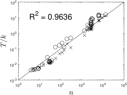
(a)

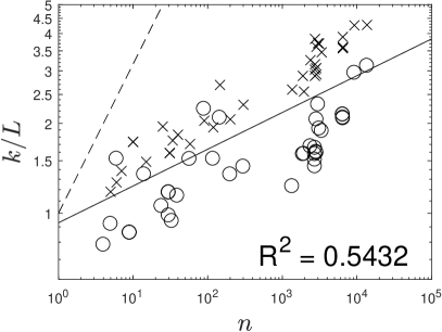
(b)

Figure 2: SeDuMi Timings for MAX $3$-CUT ($\circ$) and Lovasz Theta ($\times$) problems: (a) Time per iteration, with regression $T/k=10^{-3}n$; (b) Iterations per decimal digit of accuracy, with (solid) regression $k/L=0.929n^{0.123}$ and (dashed) bound $k/L=\sqrt{n}$.

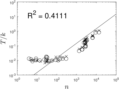
(a)

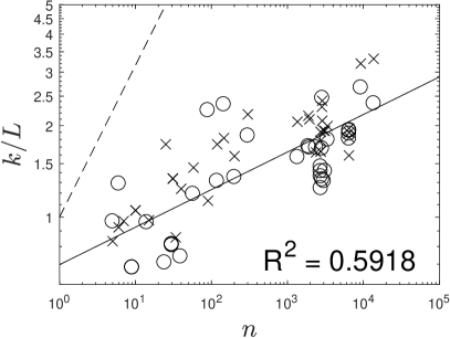
(b)

Figure 3: MOSEK Timings for MAX $3$-CUT ($\circ$) and Lovasz Theta ($\times$) problems: (a) Time per iteration, with regression $T/k=1.488\times 10^{-4}n$; (b) Iterations per decimal digit of accuracy, with (solid) regression $k/L=0.697n^{0.123}$ and (dashed) bound $k/L=\sqrt{n}$.

We begin by considering the MAX 3-CUT and Lovasz Theta problems, which are partially separable by default, and hence have solution complexities of $O(n^{1.5})$ time and $O(n)$ memory. For each of the 40 test cases, we use the MATPOWER function makeYbus to generate the bus admittance matrix $Y_{bus}=[Y_{i,j}]_{i,j=1}^{n},$ and symmetrize to yield $Y_{abs}=\frac{1}{2}[|Y_{i,j}|+|Y_{j,i}|]_{i,j=1}^{n}$. We view this matrix as the weighted adjacency matrix for the system graph. For MAX 3-CUT, we define the weighted Laplacian matrix $C=\mathrm{diag}(Y_{abs}\mathbf{1})-Y_{abs}$, and set up problem (MkC). For Lovasz Theta, we extract the location of the graph edges from $Y_{abs}$ and set up (LT^′).

First, we use Algorithm 1 with the modified version of SeDuMi to solve the 80 instances of (SDP). Of the 80 instances considered, 79 solved to $L\geq 5$ digits in $k\leq 23$ iterations and $T\leq 306$ seconds; the largest instance solved to $L=4.48$. Table 3 shows the accuracy and timing details for the 20 largest problems solved. Figure 3a plots $T/k$, the mean time taken per-iteration. As we guaranteed in Lemma 1, the per-iteration time is linear with respect to $n$. A log-log regression yields $T/k=10^{-3}n$, with $R^{2}=0.9636$. Figure 3b plots $k/L$, the number of iterations to a factor-of-ten error reduction. We see that SeDuMi’s guaranteed iteration complexity $k=O(\sqrt{n}\log\epsilon^{-1})=O(\sqrt{n}L)$ is a significant over-estimate; a log-log regression yields $k/L=0.929n^{0.123}\approx n^{1/8}$, with $R^{2}=0.5432$. Combined, the data suggests an actual time complexity of $T\approx 10^{-3}n^{1.1}L$.

Next, we use Algorithm 1 alongside the off-the-shelf version of MOSEK to solve the 80 same instances. It turns out that MOSEK is both more accurate than SeDuMi, as well as a factor of 5-10 faster. It manages to solve all 80 instances to $L\geq 6$ digits in $k\leq 21$ iterations and $T\leq 24$ seconds. Table 3 shows the accuracy and timing details for the 20 largest problems solved. Figure 3a plots $T/k$, the mean time taken per-iteration. Despite not forcing the use of a block topological ordering, MOSEK nevertheless attains an approximately linear per-iteration cost. Figure 3b plots $k/L$, the number of iterations to a factor-of-ten error reduction. Again, we see that MOSEK’s guaranteed iteration complexity $k=O(\sqrt{n}\log\epsilon^{-1})=O(\sqrt{n}L)$ is a significant over-estimate. A log-log regression yields an empirical time complexity of $T\approx 10^{-4}n^{1.12}L$, which is very close to being linear-time.

Table 2: Accuracy (in decimal digits) and timing (in seconds) for 20 largest MAX $3$-CUT problems: $n$ - order of matrix variable; $m$ - number of constraints; “Pre-proc” - post-processing time; “gap” - duality gap; “pinf” - primal infeasibility; “dinf” - dual infeasibility; $k$ - number of interior-point iterations; $T$ - total interior-point time; “Post-proc” - post-processing time.

			Pre-	MOSEK					SeDuMi					Post-
#	$n$	$m$	proc	gap	pinf	dinf	$k$	$T$	gap	pinf	dinf	$k$	$T$	proc.
21	1354	3064	1.1	9.6	8.9	9.1	14	0.6	11.6	7.5	9.7	12	17.0	0.1
22	1888	4196	1.5	8.9	8.2	8.4	14	0.8	8.2	7.1	9.4	13	24.9	0.2
23	1951	4326	1.6	8.9	8.3	8.4	14	0.8	8.9	7.3	10.1	14	46.2	0.2
24	2383	5269	2.1	9.0	8.3	8.4	14	2.2	7.8	7.3	8.5	13	37.1	0.4
25	2736	5999	2.4	8.8	8.2	8.3	12	2.0	12.0	7.5	10.6	16	99.6	0.4
26	2737	6000	2.4	9.0	8.5	8.5	12	1.9	11.4	6.8	9.7	14	47.7	0.4
27	2746	6045	2.4	11.3	10.4	10.8	13	2.4	11.3	6.4	9.5	15	69.3	0.4
28	2746	6019	2.4	10.9	10.3	10.3	14	2.2	11.9	7.1	10.3	17	117.3	0.4
29	2848	6290	2.5	8.9	8.3	8.4	14	1.2	8.1	6.9	9.4	13	46.7	0.4
30	2868	6339	2.6	10.4	9.8	9.9	13	1.2	8.2	6.9	9.5	13	49.5	0.4
31	2869	6837	2.7	8.7	8.1	8.2	20	2.0	9.6	5.2	8.2	17	84.7	0.5
32	3012	6578	2.7	9.8	9.1	9.3	12	2.5	7.8	7.3	10.1	18	157.1	0.5
33	3120	6804	2.8	9.3	8.5	8.7	12	2.6	11.7	7.7	10.4	20	166.4	0.5
34	3374	7442	3.2	9.1	8.3	8.5	15	3.6	10.0	5.8	8.5	16	124.7	0.6
35	6468	14533	7.6	9.2	8.5	8.7	16	5.6	9.4	4.9	7.5	16	210.9	1.6
36	6470	14536	7.6	9.7	8.8	9.2	16	5.6	9.4	5.0	7.5	16	218.2	1.6
37	6495	14579	7.7	9.0	8.3	8.5	16	5.6	9.4	4.7	7.6	16	193.8	1.6
38	6515	14619	7.7	9.0	8.3	8.5	16	5.6	9.8	5.3	8.2	17	257.8	1.6
39	9241	23448	14.0	9.2	8.2	8.7	22	17.6	5.1	4.1	6.6	15	187.5	3.5
40	13659	32284	23.5	9.2	8.4	8.7	20	16.3	4.5	3.8	6.0	14	216.9	6.0

Table 3: Accuracy and Timing for 20 largest Lovasz Theta problems.

			Pre-	MOSEK					SeDuMi					Post-
#	$n$	$m$	proc	gap	pinf	dinf	$k$	$T$	gap	pinf	dinf	$k$	$T$	proc.
21	1355	1711	0.8	11.6	8.3	8.8	17	1.0	6.4	5.4	6.2	16	11.7	0.2
22	1889	2309	1.2	11.4	7.9	8.4	17	1.3	5.9	5.1	6.7	17	27.0	0.3
23	1952	2376	1.2	11.2	7.6	8.1	16	1.2	6.3	5.5	6.9	16	31.6	0.3
24	2384	2887	1.6	12.2	8.6	9.1	14	3.3	5.8	5.1	6.6	19	33.9	0.4
25	2737	3264	1.8	11.4	7.9	8.4	13	3.4	6.6	5.6	6.8	19	36.9	0.5
26	2738	3264	1.8	10.9	7.3	7.8	14	3.5	7.4	5.8	6.3	19	35.3	0.5
27	2747	3300	1.8	13.2	9.1	9.8	15	4.3	5.2	4.7	6.7	20	57.6	0.6
28	2747	3274	1.9	11.4	7.8	8.4	14	3.5	7.5	5.3	5.7	18	30.5	0.5
29	2849	3443	1.9	11.1	7.4	7.8	17	2.0	8.5	5.1	5.6	17	33.3	0.5
30	2869	3472	1.9	11.4	7.7	8.2	16	1.9	5.8	4.9	6.5	17	41.4	0.5
31	2870	3969	2.0	11.1	7.5	7.9	18	3.0	6.1	5.2	6.1	22	74.0	0.6
32	3013	3567	2.1	11.4	7.8	8.3	15	4.1	9.1	5.9	5.9	22	65.5	0.6
33	3121	3685	2.2	14.6	8.9	10.5	17	5.1	8.8	5.6	5.7	21	44.5	0.7
34	3375	4069	2.4	12.6	8.5	9.7	17	6.5	9.2	5.8	6.1	21	73.1	0.8
35	6469	8066	5.5	13.7	8.8	9.4	14	7.2	5.1	4.8	6.9	20	137.0	2.1
36	6471	8067	5.5	12.2	8.2	8.7	16	7.5	5.7	4.9	5.6	20	125.9	2.1
37	6496	8085	5.6	12.9	9.0	9.4	17	7.9	5.7	4.9	5.6	20	131.4	2.0
38	6516	8105	5.6	13.2	8.8	9.3	16	7.1	5.7	4.9	5.6	20	133.9	2.1
39	9242	14208	10.0	10.4	6.2	6.7	20	20.3	6.2	4.7	5.4	23	237.2	4.6
40	13660	18626	16.4	10.8	6.3	6.7	21	23.3	5.7	4.5	5.4	23	305.9	8.0

8.3 Optimal power flow

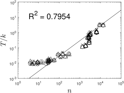
(a)

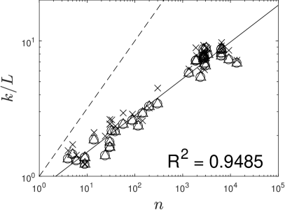
(b)

Figure 4: OPF problems solved using clique tree conversion ($\times$), dualized clique tree conversion ($\circ$) and dualized clique tree conversion with auxiliary variables ($\triangle$): (a) Time per iteration, with regression $T/k=2.931\times 10^{-4}n$; (b) Iterations per decimal digit of accuracy, with (solid) regression $k/L=0.807n^{0.271}$ and (dashed) bound $k/L=\sqrt{n}$.

Table 4: Accuracy (in decimal digits) and timing (in seconds) for 20 largest OPF problems: $n$ - order of matrix variable; $m$ - number of constraints; “Pre-proc” - post-processing time; $L=\min\{\mathrm{gap},\mathrm{pinf},\mathrm{dinf}\}$ - accurate decimal digits; $k$ - number of interior-point iterations; $T$ - total interior-point time; “Post-proc” - post-processing time.

			Pre-	CTC			Dual CTC			Dual CTC w/ aux			Post-
#	$n$	$m$	proc	$L$	$k$	$T$	$L$	$k$	$T$	$L$	$k$	$T$	proc.
21	1354	4060	3.0	7.3	45	6.9	7.2	42	4.2	7.1	41	4.5	0.2
22	1888	5662	4.1	7.2	64	11.0	6.9	48	6.3	6.8	48	6.2	0.3
23	1951	5851	4.2	7.8	61	10.9	7.1	46	6.0	7.0	50	6.7	0.3
24	2383	7147	5.9	7.2	43	30.4	6.9	38	16.6	6.9	37	16.2	0.4
25	2736	8206	7.0	7.2	60	46.2	6.8	53	23.8	6.5	48	22.3	0.5
26	2737	8209	6.8	7.1	66	45.7	6.7	57	24.5	6.9	53	23.1	0.5
27	2746	8236	7.0	6.9	50	45.1	6.6	50	24.7	6.3	47	23.9	0.5
28	2746	8236	6.9	7.1	60	44.2	6.7	56	25.2	6.9	60	26.7	0.6
29	2848	8542	6.8	7.1	56	18.9	6.4	49	10.1	6.4	48	10.2	0.5
30	2868	8602	6.8	7.4	56	18.8	6.6	51	10.6	6.7	52	10.8	0.5
31	2869	8605	7.4	7.7	47	19.6	7.1	46	12.7	7.4	50	14.1	0.6
32	3012	9034	7.9	7.0	55	54.5	6.1	54	31.6	6.9	45	28.5	0.6
33	3120	9358	8.1	7.2	64	70.7	6.3	58	38.5	6.7	59	38.2	0.7
34	3374	10120	8.9	7.1	62	69.3	6.6	56	39.8	6.6	52	39.0	0.7
35	6468	19402	17.9	7.6	64	99.9	7.0	54	53.7	6.9	53	56.7	2.0
36	6470	19408	18.0	7.4	68	106.1	6.8	57	56.3	6.9	56	57.2	2.0
37	6495	19483	17.7	7.5	66	102.8	7.3	54	53.2	7.0	60	62.3	2.0
38	6515	19543	17.7	7.2	70	103.4	6.8	54	54.7	6.8	59	58.1	2.0
39	9241	27721	31.3	7.5	64	230.1	7.0	57	165.0	7.6	55	169.7	4.3
40	13659	40975	47.9	6.8	49	177.4	7.9	48	154.6	7.9	54	157.4	7.7

We now solve instances of the OPF posed on the same 40 power systems as mentioned above. Here, we use the MATPOWER function makeYbus to generate the bus admittance matrix $Y_{bus}$, and then manually generate each constraint matrix $A_{i}$ from $Y_{bus}$ using the recipes described in lavaei2012zero . Specifically, we formulate each OPF problem given the power flow case as follows:

• Minimize the cost of generation. This is the sum of real-power injection at each generator times $1 per MW.

• Constrain all bus voltages to be from 95% to 105% of their nominal values.

• Constrain all load bus real-power and reactive-power values to be from 95% to 105% of their nominal values.

• Constrain all generator bus real-power and reactive-power values within their power curve. The actual minimum and maximum real and reactive power limits are obtained from the case description.

We use three different algorithms based to solve the resulting semidefinite program: 1) The original clique tree conversion of Fukuda and Nakata et al. fukuda2001exploiting ; nakata2003exploiting in Section 3.3; 2) Dualized clique tree conversion in Algorithm 1; 3) Dualized clique tree conversion with auxiliary variables in Algorithm 3. We solved all 40 problems using the three algorithms and MOSEK as the internal interior-point solver. Table 4 shows the accuracy and timing details for the 20 largest problems solved. All three algorithms achieved near-linear time performance, solving each problem instances to 7 digits of accuracy within 6 minutes. Upon closer examination, we see that the two dualized algorithms are both about a factor-of-two faster than the basic CTC method. Figure 4 plots $T/k$, the mean time taken per-iteration, and $k/L$, the number of iterations for a factor-of-ten error reduction, and their respective log-log regressions. The data suggests an empirical time complexity of $T\approx 2.3\times 10^{-4}n^{1.3}L$ over the three algorithms.

9 Conclusion

Clique tree conversion splits a large $n\times n$ semidefinite variable $X\succeq 0$ into up to $n$ smaller semidefinite variables $X_{j}\succeq 0$, coupled by a large number of overlap constraints. These overlap constraints are a fundamental weakness of clique tree conversion, and can cause highly sparse semidefinite program to be solved in as much as cubic time and quadratic memory.

In this paper, we apply dualization to clique tree decomposition. Under a partially separable sparsity assumption, we show that the resulting normal equations have a block-sparsity pattern that coincides with the adjacency matrix of a tree graph, so the per-iteration time and memory complexity of an interior-point method is guaranteed to be linear with respect to $n$, the order of the matrix variable $X$. Problems that do not satisfy the separable assumption can be systematically separated by introducing auxiliary variables. In the case of network flow semidefinite programs, the number of auxiliary variables can be bounded, so an interior-point method again has a per-iteration time and memory complexity that is linear with respect to $n$.

Using these insights, we prove that the MAXCUT and MAX $k$-CUT relaxations, the Lovasz Theta problem, and the AC optimal power flow relaxation can all be solved with a guaranteed time and memory complexity that is near-linear with respect to $n$, assuming that a tree decomposition with small width for the sparsity graph is known. Our numerical results confirm an empirical time complexity that is linear with respect to $n$ on the MAX 3-CUT and Lovasz Theta relaxations.

Appendix A Linear independence and Slater’s conditions

In this section, we prove that (CTC) inherits the assumptions of linear independence and Slater’s conditions from (SDP). We begin with two important technical lemmas.

Lemma 10

The matrix $\mathbf{N}$ in (13) has full row rank, that is $\det(\mathbf{N}\mathbf{N}^{T})\neq 0$.

Proof

We make $\mathbf{N}=[\mathbf{N}_{i,j}]_{i,j=1}^{\ell}$ upper-triangular by ordering its blocks topologically on $T$: each nonempty block row $\mathbf{N}_{j}$ contains a nonzero block at $\mathbf{N}_{j,j}$ and a nonzero block at $\mathbf{N}_{j,p(j)}$ where the parent node $p(j)>j$ is ordered after $j$. Then, the claim follows because each diagonal block $\mathbf{N}_{j,j}$ implements a surjection and must therefore have full row-rank. ∎

Lemma 11 (Orthogonal complement)

Let $d=\frac{1}{2}\sum_{j=1}^{\ell}|J_{j}|(|J_{j}|+1)$. Implicitly define the $d\times\frac{1}{2}n(n+1)$ matrix $\mathbf{P}$ to satisfy

$$\mathbf{P}\,\mathrm{svec}\,(X) =[\mathrm{svec}\,(X[J_{1},J_{1}]);\ldots;\mathrm{svec}\,(X[J_{\ell},J_{\ell}])]\qquad\forall X\in\mathbb{S}^{n}.$$

Then, (i) $\mathbf{N}\mathbf{P}=0$; (ii) every $x\in\mathbb{R}^{d}$ can be decomposed as $x=\mathbf{N}^{T}u+\mathbf{P}v$.

Proof

For each $x=[\mathrm{svec}\,(X_{j})]_{j=1}^{\ell}\in\mathbb{R}^{d}$, Theorem 3.2 says that there exists a $Z$ satisfying $\mathbf{P}\,\mathrm{svec}\,(Z)=x$ if and only if $\mathbf{N}x=0$. Equivalently, $x\in\mathrm{span}(\mathbf{P})$ if and only if $x\perp\mathrm{span}(\mathbf{N}^{T})$. The “only if” part implies (i), while the “if” part implies (ii).

Define the $m\times\frac{1}{2}n(n+1)$ matrix $\mathbf{M}$ as the vectorization of the linear constraints in (SDP), as in

$$\mathbf{M}\,\mathrm{svec}\,(X)=\begin{bmatrix}\mathrm{svec}\,(A_{1})^{T}\\ \vdots\\ \mathrm{svec}\,(A_{m})^{T}\end{bmatrix}\mathrm{svec}\,(X)=\begin{bmatrix}\mathrm{svec}\,(A_{1})^{T}\mathrm{svec}\,(X)\\ \vdots\\ \mathrm{svec}\,(A_{m})^{T}\mathrm{svec}\,(X)\end{bmatrix}=\begin{bmatrix}A_{1}\bullet X\\ \vdots\\ A_{m}\bullet X\end{bmatrix}.$$

In reformulating (SDP) into (CTC), the splitting conditions (10) can be rewritten as the following

$$c^{T}\mathbf{P} =\mathrm{svec}\,(C)^{T}, \mathbf{A}\mathbf{P} =\mathbf{M},$$ (38)

where $c=[\mathrm{svec}\,(C_{j})]_{j=1}^{\ell}$ and $\mathbf{A}=[\mathrm{svec}\,(A_{i,j})^{T}]_{i,j=1}^{m,\ell}$ are the data for the vectorized verison of (CTC).

Proof (Lemma 1)

We will prove that

$$\text{exists }[u;v]\neq 0,\quad\mathbf{A}^{T}u+\mathbf{N}^{T}v=0\qquad\iff\qquad\text{exists }y\neq 0,\quad\sum_{i=1}^{m}y_{i}A_{i}=0.$$

($\implies$) We must have $u\neq 0$, because $\mathbf{N}$ has full row rank by Lemma 10, and so $\mathbf{A}^{T}0+\mathbf{N}^{T}v=0$ if and only if $v=0$. Multiplying by $\mathbf{P}$ yields $\mathbf{P}^{T}(\mathbf{A}^{T}u+\mathbf{N}^{T}v)=\mathbf{M}^{T}u+0=0$ and so setting $y=u\neq 0$ yields $\mathbf{M}^{T}y=0$. ($\impliedby$) We use Lemma 11 to decompose $\mathbf{A}^{T}y=\mathbf{P}z+\mathbf{N}^{T}v$. If $\mathrm{svec}\,(\sum_{i}y_{i}A_{i})=\mathbf{M}^{T}y=\mathbf{P}^{T}\mathbf{A}^{T}y=0,$ then $\mathbf{P}^{T}\mathbf{P}z=\mathbf{P}^{T}\mathbf{A}^{T}y-\mathbf{P}^{T}\mathbf{N}^{T}v=0$ and so $\mathbf{P}z=0$. Setting $u=-y\neq 0$ yields $\mathbf{A}^{T}u+\mathbf{N}^{T}v=0$.∎

Proof (Lemma 2)

We will prove that

$$\text{exists }x\in\mathrm{Int}(\mathcal{K}),\quad\begin{bmatrix}\mathbf{A}\\ \mathbf{N}\end{bmatrix}x=\begin{bmatrix}b\\ 0\end{bmatrix}\qquad\iff\qquad\text{exists }X\succeq 0,\quad\mathbf{M}\,\mathrm{svec}\,(X)=b.$$

Define the chordal completion $F$ as in (8). Observe that $\mathbf{M}\,\mathrm{svec}\,(X)=\mathbf{M}\,\mathrm{svec}\,(Z)$ holds for all pairs of $P_{F}(X)=Z$, because each $A_{i}\in\mathbb{S}_{F}^{n}$ satisfies $A_{i}\bullet X=A_{i}\bullet P_{F}(X)$. Additionally, the positive definite version of Theorem 3.1 is written

$$\text{exists }X\succ 0,\quad P_{F}(X)=Z\qquad\iff\qquad\mathbf{P}\,\mathrm{svec}\,(Z)\in\mathrm{Int}(\mathcal{K}).$$ (39)

This result was first established by Grone et al. grone1984positive ; a succinct proof can be found in (vandenberghe2015chordal, , Theorem 10.1). ($\implies$) For every $x$ satisfying $\mathbf{N}x=0$, there exists $Z$ such that $\mathbf{P}\,\mathrm{svec}\,(Z)=x$ due to Lemma 11. If additionally $x\in\mathrm{Int}(\mathcal{K})$, then there exists $X\succ 0$ satisfying $Z=P_{F}(X)$ due to (39). We can verify that $\mathbf{M}\,\mathrm{svec}\,(X)=\mathbf{M}\,\mathrm{svec}\,(Z)=\mathbf{A}\mathbf{P}\,\mathrm{svec}\,(Z)=\mathbf{A}x=b$. ($\impliedby$) For every $X\succ 0,$ there exists $Z$ satisfying $Z=P_{F}(X)$ and $\mathbf{P}\,\mathrm{svec}\,(Z)\in\mathrm{Int}(\mathcal{K})$ due to (39). Set $u=\mathbf{P}\,\mathrm{svec}\,(Z)$ and observe that $u\in\mathrm{Int}(\mathcal{K})$ and $\mathbf{N}u=\mathbf{N}\mathbf{P}\,\mathrm{svec}\,(Z)=0$. If additionally $\mathbf{M}\,\mathrm{svec}\,(X)=b$, then $\mathbf{A}u=\mathbf{A}\mathbf{P}\,\mathrm{svec}\,(Z)=\mathbf{M}\,\mathrm{svec}\,(Z)=b$.∎

Proof (Lemma 2)

We will prove that

$$\text{exists }u,v,\quad c-\mathbf{A}^{T}u-\mathbf{N}^{T}v\in\mathrm{Int}(\mathcal{K}_{*})\qquad\iff\qquad\text{exists }y,\quad C-\sum_{i}y_{i}A_{i}\succ 0.$$

Define the chordal completion $F$ as in (8). Theorem 3.1 in (39) has a dual theorem

$$\text{exists }S\succ 0,\quad S\in\mathbb{S}_{F}^{n}\qquad\iff\qquad\text{exists }h\in\mathrm{Int}(\mathcal{K}_{*}),\quad\mathrm{svec}\,(S)=\mathbf{P}^{T}h.$$ (40)

This result readily follows from the positive semidefinite version proved by Alger et al. agler1988positive ; see also (vandenberghe2015chordal, , Theorem 9.2). ($\implies$) For each $h=c-\mathbf{A}^{T}u-\mathbf{N}^{T}v$, define $S=C-\sum_{i}u_{i}A_{i}$ and observe that

$$\mathbf{P}^{T}h=\mathbf{P}^{T}(c-\mathbf{A}^{T}u-\mathbf{N}^{T}v)=\mathrm{svec}\,(C)-\mathbf{M}^{T}u-0=\mathrm{svec}\,(S).$$

If additionally $h\in\mathcal{K}_{*}$, then $S\succ 0$ due to (40). ($\impliedby$) For each $S=C-\sum_{i}y_{i}A_{i}\succ 0$, there exists an $h\in\mathrm{Int}(\mathcal{K}_{*})$ satisfying $\mathrm{svec}\,(S)=\mathbf{P}^{T}h$ due to (40). We use Lemma 11 to decompose $h=\mathbf{P}u+\mathbf{N}^{T}v$. Given that $\mathrm{svec}\,(S)=\mathbf{P}^{T}h=\mathbf{P}^{T}\mathbf{P}u+0$, we must actually have $\mathbf{P}u=c-\mathbf{A}^{T}y$ since $\mathbf{P}^{T}(c-\mathbf{A}^{T}y)=\mathrm{svec}\,(C)-\mathbf{M}^{T}y=\mathrm{svec}\,(S)$. Hence $h=c-\mathbf{A}^{T}y+\mathbf{N}^{T}v$ and $h\in\mathrm{Int}(\mathcal{K}_{*})$.∎

Appendix B Extension to inequality constraints

Consider the modifying the equality constraint in (11) into an inequality constraint, as in

$$\text{minimize }c^{T}x\quad\text{subject to }\quad\mathbf{A}x\leq b,\quad\mathbf{N}x=0,\quad x\in\mathcal{K}.$$

The corresponding dualization reads

$$\text{maximize }-c^{T}y\quad\text{subject to }\quad\begin{bmatrix}\mathbf{A}\\ \mathbf{N}\\ -I\end{bmatrix}y+s=\begin{bmatrix}b\\ 0\\ 0\end{bmatrix},\quad s\in\mathbb{R}_{+}^{m}\times\{0\}^{f}\times\mathcal{K},$$

where $m$ denotes the number of rows in $\mathbf{A}$ and $f$ now denotes the number of rows in $\mathbf{N}$. Embedding the equality constraint into a second-order cone, the associated normal equation takes the form

$$\left(\mathbf{D}_{s}+\mathbf{A}^{T}\mathbf{D}_{l}\mathbf{A}+\mathbf{N}^{T}\mathbf{D}_{f}\mathbf{N}\right)\Delta y=r,$$

where $\mathbf{D}_{s}$ and $\mathbf{D}_{f}$ are comparable as before in (15) and (23), and $\mathbf{D}_{l}$ is a diagonal matrix with positive diagonal elements. This matrix has the same sparse-plus-rank-1 structure as (22), and can therefore be solved using the same rank-1 update

$$\Delta y=(\mathbf{H}+\mathbf{q}\mathbf{q}^{T})^{-1}r=\left(I-\frac{(\mathbf{H}^{-1}\mathbf{q})\mathbf{q}^{T}}{1+\mathbf{q}^{T}(\mathbf{H}^{-1}\mathbf{q})}\right)\mathbf{H}^{-1}r,$$

where $\mathbf{H}$ and $\mathbf{q}$ now read

$$\mathbf{H} =\mathbf{D}_{s}+\mathbf{A}^{T}\mathbf{D}_{l}\mathbf{A}+\sigma\mathbf{N}^{T}\mathbf{N}, \mathbf{q} =\mathbf{N}^{T}w.$$

The matrix $\mathbf{H}$ has the same block sparsity graph as the tree graph $T$, so we can evoke Lemma 5 to show that the cost of computing $\Delta y$ is again $O(\omega^{6}n)$ time and $O(\omega^{4}n)$ memory.

Appendix C Interior-point method complexity analysis

We solve the dualized problem (21) by solving its extended homogeneous self-dual embedding

min. $$(\nu+1)\theta$$ (41a)

s.t. $$\begin{bmatrix}0&+\mathbf{M}^{T}&-\mathbf{c}&-r_{d}\\ -\mathbf{M}&0&+\mathbf{b}&-r_{p}\\ +\mathbf{c}^{T}&-\mathbf{b}^{T}&0&-r_{c}\\ r_{d}^{T}&r_{p}^{T}&r_{c}&0\end{bmatrix}\begin{bmatrix}x\\ y\\ \tau\\ \theta\end{bmatrix}+\begin{bmatrix}s\\ 0\\ \kappa\\ 0\end{bmatrix} =\begin{bmatrix}0\\ 0\\ 0\\ \nu+1\end{bmatrix}$$ (41b)

$$x,s\in\mathcal{C}\quad\kappa,\tau \geq 0,$$ (41c)

where the data is given in standard form

$$\mathbf{M}=\begin{bmatrix}0&-\begin{bmatrix}\mathbf{A}^{T}&\mathbf{N}^{T}\end{bmatrix}&+I\end{bmatrix},\quad\mathbf{c}^{T}=\begin{bmatrix}0&\begin{bmatrix}b^{T}&0\end{bmatrix}&0\end{bmatrix},\quad\mathbf{b}=-c,$$ (41d)

$$\mathcal{C}=\{(x_{0},x_{1}\}\in\mathbb{R}^{p+1}:\|x_{1}\|\leq x_{0}\}\times\mathcal{K},$$ (41e)

and the residual vectors are defined

$$r_{d}=\mathbf{1}_{\mathcal{C}}-\mathbf{c},\quad r_{p}=-\mathbf{M}\mathbf{1}_{\mathcal{C}}+\mathbf{b},\quad r_{c}=1+\mathbf{c}^{T}\mathbf{1}_{\mathcal{C}}.$$ (41f)

Here, $\nu$ is the order of the cone $\mathcal{C}$, and $\mathbf{1}_{\mathcal{C}}$ is its identity element

$$\nu =1+|J_{1}|+\cdots+|J_{\ell}|, \mathbf{1}_{\mathcal{C}} =[1;0;\ldots;0;\mathrm{svec}\,(I_{|J_{1}|});\ldots;\mathrm{svec}\,(I_{|J_{\ell}|})].$$ (42)

Problem (41) has optimal value $\theta^{\star}=0$. Under the primal-dual Slater’s conditions (Assumption 2), an interior-point method is guaranteed to converge to an $\epsilon$-accurate solution with $\tau>0$, and this yields an $\epsilon$-feasible and $\epsilon$-accurate solution to the dualized problem (21) by rescaling $x/\tau$ and $y=y/\tau$ and $s=s/\tau$. The following result is adapted from (de2000self, , Lemma 5.7.2) and (vanderbei2015linear, , Theorem 22.7).

Lemma 12 ($\epsilon$-accurate and $\epsilon$-feasible)

If $(x,y,s,\tau,\theta,\kappa)$ satisfies (41b) and (41c) and

$$\mu=\frac{x^{T}s+\tau\kappa}{\nu+1} \leq\epsilon, \tau\kappa\geq \gamma\mu$$

for constants $\epsilon,\gamma>0$, then the rescaled point $(x/\tau,y/\tau,s/\tau)$ satisfies

$$\|\mathbf{M}(x/\tau)-\mathbf{b}\| \leq K\epsilon, \|\mathbf{M}^{T}(y/\tau)+(s/\tau)-\mathbf{c}\| \leq K\epsilon, \frac{(x/\tau)^{T}(s/\tau)}{\nu+1}\leq K\epsilon$$

where $K$ is a constant.

Proof

Note that (41b) implies $\mu=\theta$ and

$$\|\mathbf{M}(x/\tau)-\mathbf{b}\| =\frac{\|r_{p}\|\mu}{\tau}, \|\mathbf{M}^{T}(y/\tau)+(s/\tau)-\mathbf{c}\| =\frac{\|r_{d}\|\mu}{\tau}, \frac{(x/\tau)^{T}(s/\tau)}{\nu+1}=\frac{\mu}{\tau^{2}}.$$

Hence, we obtain our desired result by upper-bounding $1/\tau$. Let $(x^{\star},y^{\star},s^{\star},\tau^{\star},\theta^{\star},\kappa^{\star})$ be a solution of (41), and note that for every $(x,y,s,\tau,\theta,\kappa)$ satisfying (41b) and (41c), we have the following via the skew-symmetry of (41b)

$$(x-x^{\star})^{T}(s-s^{\star})+(\tau-\tau^{\star})(\kappa-\kappa^{\star})=0.$$

Rearranging yields

$$(\nu+1)\mu=x^{T}s+\tau\kappa=(x^{\star})^{T}s+x^{T}(s^{\star})+\tau\kappa^{\star}+\tau^{\star}\kappa\geq\tau^{\star}\kappa$$

and hence

$$\kappa\tau^{\star}\leq\mu(\nu+1),\quad\tau\kappa\geq\gamma\mu\qquad\implies\qquad\tau\geq\frac{\gamma}{\nu+1}\tau^{\star}.$$

If (SDP) satisfies the primal-dual Slater’s condition, then (CTC) also satisfies the primal-dual Slater’s condition (Lemmas 2 & 3). Therefore, the vectorized version (11) of (CTC) attains a solution $(\hat{x},\hat{y},\hat{s})$ with $\hat{x}^{T}\hat{s}=0$, and the following

$$x^{\star}=\tau^{\star}\begin{bmatrix}\|\hat{y}\|\\ \hat{y}\\ \hat{s}\end{bmatrix},\quad y^{\star}=\tau^{\star}\hat{x},\quad s^{\star}=\tau^{\star}\begin{bmatrix}0\\ 0\\ \hat{x}\end{bmatrix},\quad\tau^{\star}=\frac{\nu+1}{\|\hat{y}\|+\mathbf{1}_{\mathcal{K}}^{T}\hat{s}+\mathbf{1}_{\mathcal{K}}^{T}\hat{x}+1},$$

with $\theta^{\star}=\kappa^{\star}=0$ is a solution to (41). This proves the following upper-bound

$$\frac{1}{\tau}\leq K_{\tau}=\frac{1}{\gamma}\cdot\min_{\hat{x},\hat{y},\hat{s}}\{\|\hat{y}\|+\mathbf{1}_{\mathcal{K}}^{T}\hat{s}+\mathbf{1}_{\mathcal{K}}^{T}\hat{x}+1:(\hat{x},\hat{y},\hat{s})\text{ solves (\ref{eq:vecCTC}) with }\hat{x}^{T}\hat{s}=0\}.$$

Setting $K=\max\{\|r_{p}\|K_{\tau},\|r_{d}\|K_{\tau},K_{\tau}^{2}\}$ yields our desired result. ∎

We solve the homogeneous self-dual embedding (41) using the short-step method of Nesterov and Todd (nesterov1998primal, , Algorithm 6.1) (and also Sturm and S. Zhang (sturm1999symmetric, , Section 5.1)), noting that SeDuMi reduces to it in the worst case; see sturm2002implementation and sturm1997wide . Beginning at the following strictly feasible, perfectly centered point

$$\theta^{(0)}=\tau^{(0)}=\kappa^{(0)}=1,\quad y^{(0)}=0,\quad x^{(0)}=s^{(0)}=\mathbf{1}_{\mathcal{C}},$$ (43)

with barrier parameter $\mu=1$, we take the following steps

$$\mu^{+} =\left(1-\frac{1}{15\sqrt{\nu+1}}\right)\cdot\frac{x^{T}s+\tau\kappa}{\nu+1},$$ (44a)

$$(x^{+},y^{+},s^{+},\tau^{+},\theta^{+},\kappa^{+}) =(x,y,s,\tau,\theta,\kappa)+(\Delta x,\Delta y,\Delta s,\Delta\tau,\Delta\theta,\Delta\kappa).$$

along the search direction defined by the linear system (todd1998nesterov, , Eqn. 9)

$$\begin{bmatrix}0&+\mathbf{M}^{T}&-\mathbf{c}&-r_{p}\\ -\mathbf{M}&0&+\mathbf{b}&-r_{d}\\ +\mathbf{c}^{T}&-\mathbf{b}^{T}&0&-r_{c}\\ +r_{p}^{T}&+r_{d}^{T}&+r_{c}&0\end{bmatrix}\begin{bmatrix}\Delta x\\ \Delta y\\ \Delta\tau\\ \Delta\theta\end{bmatrix}+\begin{bmatrix}\Delta s\\ 0\\ \Delta\kappa\\ 0\end{bmatrix} =0,$$ (45a)

$$s+\Delta s+\nabla^{2}F(w)\Delta x+\mu^{+}\nabla F(x) =0,$$ (45b)

$$\kappa+\Delta\kappa+(\kappa/\tau)\Delta\tau-\mu^{+}\tau^{-1} =0.$$ (45c)

Here, $F$ is the usual self-concordant barrier function on $\mathcal{C}$

$$F([x_{0};x_{1};\mathrm{svec}\,(X_{1});\ldots;\mathrm{svec}\,(X_{\ell})])= -\log\left(\frac{1}{2}x_{0}^{2}-\frac{1}{2}x_{1}^{T}x_{1}\right)-\sum_{j=1}^{\ell}\log\det(X_{j})$$ (46)

and $w\in\mathrm{Int}(\mathcal{C})$ is the unique scaling point satisfying $\nabla^{2}F(w)x=s$, which can be computed from $x$ and $s$ in closed-form. The following iteration bound is an immediate consequence of (nesterov1998primal, , Theorem 6.4); see also (sturm1999symmetric, , Theorem 5.1).

Lemma 13 (Short-Step Method)

The sequence in (44) arrives at an iterate $(x,y,s,\tau,\theta,\kappa)$ satisfying the conditions of Lemma 12 with $\gamma=9/10$ in at most $O(\sqrt{\nu}\log(1/\epsilon))$ iterations.

The cost of each interior-point iteration is dominated by the cost of computing the search direction in (45). Using elementary but tedious linear algebra, we can show that if

$$(\mathbf{M}\mathbf{D}^{-1}\mathbf{M}^{T})\begin{bmatrix}v_{1}&v_{2}&v_{3}\end{bmatrix}=\begin{bmatrix}0&-\mathbf{b}&r_{p}\end{bmatrix}-\mathbf{M}\mathbf{D}^{-1}\begin{bmatrix}d&\mathbf{c}&r_{d}\end{bmatrix}$$ (47a)

where $$\mathbf{D}=\nabla^{2}F(w) d=-s-\mu^{+}\nabla F(x)$$ and , and

$$\begin{bmatrix}u_{1}&u_{2}&u_{3}\end{bmatrix}=\mathbf{D}^{-1}(\begin{bmatrix}d&c&r_{d}\end{bmatrix}+\mathbf{M}^{T}\begin{bmatrix}v_{1}&v_{2}&v_{3}\end{bmatrix}),$$ (47b)

then

$$\left(\begin{bmatrix}-\mathbf{D}_{0}&-r_{c}\\ r_{c}&0\end{bmatrix}-\begin{bmatrix}\mathbf{c}&r_{d}\\ -\mathbf{b}&r_{p}\end{bmatrix}^{T}\begin{bmatrix}u_{2}&u_{3}\\ v_{2}&v_{3}\end{bmatrix}\right)\begin{bmatrix}\Delta\tau\\ \Delta\theta\end{bmatrix} =\begin{bmatrix}-d_{0}\\ 0\end{bmatrix}-\begin{bmatrix}\mathbf{c}&r_{d}\\ -\mathbf{b}&r_{p}\end{bmatrix}^{T}\begin{bmatrix}u_{1}\\ v_{1}\end{bmatrix},$$ (47c)

$$\begin{bmatrix}\Delta x\\ \Delta y\end{bmatrix} =\begin{bmatrix}u_{1}\\ v_{1}\end{bmatrix}-\begin{bmatrix}u_{1}&u_{2}\\ v_{1}&v_{2}\end{bmatrix}\begin{bmatrix}\Delta\tau\\ \Delta\theta\end{bmatrix},$$ (47d)

$$\Delta s =d-\mathbf{D}\Delta x,$$ (47e)

$$\Delta\kappa =d_{0}-\mathbf{D}_{0}\Delta\tau,$$ (47f)

where $\mathbf{D}_{0}=\kappa/\tau$ and $d_{0}=-\kappa+\mu^{+}\tau^{-1}$. Hence, the cost of computing the search direction is dominated by the cost of solving the normal equation for three different right-hand sides. Here, the normal matrix is written

$$\mathbf{M}\mathbf{D}^{-1}\mathbf{M}^{T}=\mathrm{diag}(W_{1}\otimes_{s}W_{1},\ldots,W_{\ell}\otimes_{s}W_{\ell})+\begin{bmatrix}\mathbf{A}\\ \mathbf{N}\end{bmatrix}^{T}(w_{1}w_{1}^{T}+\sigma I)\begin{bmatrix}\mathbf{A}\\ \mathbf{N}\end{bmatrix},$$

where $\sigma=\frac{1}{2}(w_{0}^{2}-w_{1}^{T}w_{1})>0$ and $\otimes_{s}$ denotes the symmetric Kronecker product alizadeh1998primal implicitly defined to satisfy

$$(A\otimes_{s}B)\mathrm{svec}\,(X)=\frac{1}{2}\mathrm{svec}\,(AXB^{T}+BXA^{T})\qquad\text{for all }X=X^{T}.$$

Under the hypothesis on $\mathbf{A}$ stated in Theorem 5.1, the normal matrix satisfies the assumptions of Lemma 5, and can therefore be solved in linear $O(n)$ time and memory.

Proof (Theorem 5.1)

Combining Lemma 12 and Lemma 13 shows that the desired $\epsilon$-accurate, $\epsilon$-feasible iterate is obtained after $O(\sqrt{\nu}\log(1/\epsilon))$ interior-point iterations. At each iteration we perform the following steps: 1) compute the scaling point $w$; 2) solve the normal equation (47a) for three right-hand sides; 3) back-substitute (47b)-(47f) for the search direction and take the step in (44). Note from the proof of Lemma 5 that the matrix $[\mathbf{A};\mathbf{N}]$ has at most $O(\omega^{2}n)$ rows under Assumption 1, and therefore $\mathrm{nnz}\,(\mathbf{M})=O(\omega^{4}n)$ under the hypothesis of Theorem 5.1. Below, we show that the cost of each step is bounded by $O(\omega^{6}n)$ time and $O(\omega^{4}n)$ memory.

Scaling point. We partition $x=[x_{0};x_{1};\mathrm{svec}\,(X_{1});\ldots;\mathrm{svec}\,(X_{\ell})]$ and similarly for $s$. Then, the scaling point $w$ is given in closed-form (sturm2002implementation, , Section 5)

$$\begin{bmatrix}u_{0}\\ u_{1}\end{bmatrix}=2^{-3/4}\begin{bmatrix}1&1\\ -s_{1}/\|s_{1}\|&s_{1}/\|s_{1}\|\end{bmatrix}\begin{bmatrix}(s_{0}-\|s_{1}\|)^{1/2}\\ (s_{0}+\|s_{1}\|)^{1/2}\end{bmatrix},\quad\begin{bmatrix}v_{0}\\ v_{1}\end{bmatrix}=\begin{bmatrix}u_{0}&u_{1}^{T}\\ u_{1}&\frac{1}{2}(u_{0}^{2}-u_{1}^{T}u_{1})I\end{bmatrix}\begin{bmatrix}x_{0}\\ x_{1}\end{bmatrix},$$

$$\begin{bmatrix}w_{0}\\ w_{1}\end{bmatrix}=2^{-1/4}\begin{bmatrix}u_{0}&u_{1}^{T}\\ u_{1}&\frac{1}{2}(u_{0}^{2}-u_{1}^{T}u_{1})I\end{bmatrix}\begin{bmatrix}1&1\\ -v_{1}/\|v_{1}\|&v_{1}/\|v_{1}\|\end{bmatrix}\begin{bmatrix}(v_{0}-\|v_{1}\|)^{-1/2}\\ (v_{0}+\|v_{1}\|)^{-1/2}\end{bmatrix},$$

$$W_{j}=S_{j}^{1/2}(S_{j}^{1/2}X_{j}S_{j}^{1/2})^{-1/2}S_{j}^{1/2}\qquad\text{for all }j\in\{1,\ldots,\ell\}.$$

Noting that $\mathrm{nnz}\,(w_{1})\leq O(\omega^{2}n)$, $\ell\leq n$ and each $W_{j}$ is at most $\omega\times\omega$, the cost of forming $w=[w_{0};w_{1};\mathrm{svec}\,(W_{1});\ldots;\mathrm{svec}\,(W_{\ell})]$ is at most $O(\omega^{3}n)$ time and $O(\omega^{2}n)$ memory. Also, since

$$\mathbf{D}=\nabla^{2}F(w)=\mathrm{diag}\left(\begin{bmatrix}w_{0}&w_{1}^{T}\\ w_{1}&\frac{1}{2}(w_{0}^{2}-w_{1}^{T}w_{1})I\end{bmatrix},W_{1}\otimes_{s}W_{1},\ldots,W_{\ell}\otimes_{s}W_{\ell}\right)^{-1},$$

the cost of each matrix-vector product with $\mathbf{D}$ and $\mathbf{D}^{-1}$ is also $O(\omega^{3}n)$ time and $O(\omega^{2}n)$ memory.

Normal equation. The cost of matrix-vector products with $\mathbf{M}$ and $\mathbf{M}^{T}$ is $\mathrm{nnz}\,(\mathbf{M})=O(\omega^{4}n)$ time and memory. Using Lemma 5, we form the right-hand sides and solve the three normal equations in (47a) in $O(\omega^{6}n)$ time and $O(\omega^{4}n)$ memory.

Back-substitution. The cost of back substituting (47b)-(47f) and making the step (44) is dominated by matrix-vector products with $\mathbf{D}$, $\mathbf{D}^{-1}$, $\mathbf{M}$, and $\mathbf{M}^{T}$ at $O(\omega^{4}n)$ time and memory.∎

References

- (1) L. Lovász, “On the Shannon capacity of a graph,” IEEE Transactions on Information Theory 25(1), pp. 1–7, 1979.
- (2) M. X. Goemans and D. P. Williamson, “Improved approximation algorithms for maximum cut and satisfiability problems using semidefinite programming,” Journal of the ACM 42(6), pp. 1115–1145, 1995.
- (3) H. D. Sherali and W. P. Adams, “A hierarchy of relaxations between the continuous and convex hull representations for zero-one programming problems,” SIAM Journal on Discrete Mathematics 3(3), pp. 411–430, 1990.
- (4) L. Lovász and A. Schrijver, “Cones of matrices and set-functions and 0–1 optimization,” SIAM Journal on Optimization 1(2), pp. 166–190, 1991.
- (5) J. B. Lasserre, “An explicit exact SDP relaxation for nonlinear 0-1 programs,” in International Conference on Integer Programming and Combinatorial Optimization, pp. 293–303, Springer, 2001.
- (6) M. Laurent, “A comparison of the Sherali-Adams, Lovász-Schrijver, and Lasserre relaxations for 0–1 programming,” Mathematics of Operations Research 28(3), pp. 470–496, 2003.
- (7) J. B. Lasserre, “Global optimization with polynomials and the problem of moments,” SIAM Journal on Optimization 11(3), pp. 796–817, 2001.
- (8) P. A. Parrilo, Structured semidefinite programs and semialgebraic geometry methods in robustness and optimization. PhD thesis, California Institute of Technology, 2000.
- (9) Y. Nesterov, Introductory lectures on convex optimization: A basic course, vol. 87, Springer Science & Business Media, 2013.
- (10) M. Fukuda, M. Kojima, K. Murota, and K. Nakata, “Exploiting sparsity in semidefinite programming via matrix completion I: General framework,” SIAM Journal on Optimization 11(3), pp. 647–674, 2001.
- (11) D. K. Molzahn, J. T. Holzer, B. C. Lesieutre, and C. L. DeMarco, “Implementation of a large-scale optimal power flow solver based on semidefinite programming,” IEEE Transactions on Power Systems 28(4), pp. 3987–3998, 2013.
- (12) R. Madani, S. Sojoudi, and J. Lavaei, “Convex relaxation for optimal power flow problem: Mesh networks,” IEEE Transactions on Power Systems 30(1), pp. 199–211, 2015.
- (13) R. Madani, M. Ashraphijuo, and J. Lavaei, “Promises of conic relaxation for contingency-constrained optimal power flow problem,” IEEE Transactions on Power Systems 31(2), pp. 1297–1307, 2016.
- (14) A. Eltved, J. Dahl, and M. S. Andersen, “On the robustness and scalability of semidefinite relaxation for optimal power flow problems,” Optimization and Engineering , Mar 2019.
- (15) L. Vandenberghe, M. S. Andersen, et al., “Chordal graphs and semidefinite optimization,” Foundations and Trends in Optimization 1(4), pp. 241–433, 2015.
- (16) Y. Sun, M. S. Andersen, and L. Vandenberghe, “Decomposition in conic optimization with partially separable structure,” SIAM Journal on Optimization 24(2), pp. 873–897, 2014.
- (17) M. S. Andersen, A. Hansson, and L. Vandenberghe, “Reduced-complexity semidefinite relaxations of optimal power flow problems,” IEEE Transactions on Power Systems 29(4), pp. 1855–1863, 2014.
- (18) J. Löfberg, “Dualize it: software for automatic primal and dual conversions of conic programs,” Optimization Methods and Software 24(3), pp. 313–325, 2009.
- (19) A. Griewank and P. L. Toint, “Partitioned variable metric updates for large structured optimization problems,” Numerische Mathematik 39(1), pp. 119–137, 1982.
- (20) M. Andersen, J. Dahl, and L. Vandenberghe, “CVXOPT: A Python package for convex optimization,” abel.ee.ucla.edu/cvxopt , 2013.
- (21) J. Löfberg, “Yalmip: A toolbox for modeling and optimization in matlab,” in Proceedings of the CACSD Conference, 3, Taipei, Taiwan, 2004.
- (22) K. Fujisawa, S. Kim, M. Kojima, Y. Okamoto, and M. Yamashita, “User’s manual for SparseCoLO: Conversion methods for sparse conic-form linear optimization problems,” tech. rep., Department of Mathematical and Computing Sciences, Tokyo Institute of Technology, 2009. Research Report B-453.
- (23) S. Kim, M. Kojima, M. Mevissen, and M. Yamashita, “Exploiting sparsity in linear and nonlinear matrix inequalities via positive semidefinite matrix completion,” Mathematical Programming 129(1), pp. 33–68, 2011.
- (24) M. S. Andersen, “Opfsdr v0.2.3,” 2018.
- (25) R. Madani, A. Kalbat, and J. Lavaei, “ADMM for sparse semidefinite programming with applications to optimal power flow problem,” in IEEE 54th Annual Conference on Decision and Control (CDC), pp. 5932–5939, IEEE, 2015.
- (26) Y. Zheng, G. Fantuzzi, A. Papachristodoulou, P. Goulart, and A. Wynn, “Chordal decomposition in operator-splitting methods for sparse semidefinite programs,” Mathematical Programming , pp. 1–44, 2019.
- (27) M. Annergren, S. Khoshfetrat Pakazad, A. Hansson, and B. Wahlberg, “A distributed primal-dual interior-point method for loosely coupled problems using admm,” arXiv preprint arXiv:1406.2192 , 2014.
- (28) S. Khoshfetrat Pakazad, A. Hansson, and M. S. Andersen, “Distributed interior-point method for loosely coupled problems,” IFAC Proceedings Volumes 47(3), pp. 9587–9592, 2014.
- (29) R. Y. Zhang and J. K. White, “Gmres-accelerated admm for quadratic objectives,” SIAM Journal on Optimization 28(4), pp. 3025–3056, 2018.
- (30) M. S. Andersen, J. Dahl, and L. Vandenberghe, “Implementation of nonsymmetric interior-point methods for linear optimization over sparse matrix cones,” Mathematical Programming Computation 2(3), pp. 167–201, 2010.
- (31) I. S. Duff and J. K. Reid, “The multifrontal solution of indefinite sparse symmetric linear,” ACM Transactions on Mathematical Software (TOMS) 9(3), pp. 302–325, 1983.
- (32) J. W. Liu, “The multifrontal method for sparse matrix solution: Theory and practice,” SIAM review 34(1), pp. 82–109, 1992.
- (33) S. Khoshfetrat Pakazad, A. Hansson, M. S. Andersen, and I. Nielsen, “Distributed primal–dual interior-point methods for solving tree-structured coupled convex problems using message-passing,” Optimization Methods and Software 32(3), pp. 401–435, 2017.
- (34) S. Khoshfetrat Pakazad, A. Hansson, M. S. Andersen, and A. Rantzer, “Distributed semidefinite programming with application to large-scale system analysis,” IEEE Transactions on Automatic Control 63(4), pp. 1045–1058, 2017.
- (35) F. Alizadeh, J.-P. A. Haeberly, and M. L. Overton, “Complementarity and nondegeneracy in semidefinite programming,” Mathematical programming 77(1), pp. 111–128, 1997.
- (36) S. Arnborg, D. G. Corneil, and A. Proskurowski, “Complexity of finding embeddings in a k-tree,” SIAM Journal on Algebraic Discrete Methods 8(2), pp. 277–284, 1987.
- (37) Y. Ye, M. J. Todd, and S. Mizuno, “An -iteration homogeneous and self-dual linear programming algorithm,” Mathematics of Operations Research 19(1), pp. 53–67, 1994.
- (38) E. de Klerk, T. Terlaky, and K. Roos, “Self-dual embeddings,” in Handbook of Semidefinite Programming, pp. 111–138, Springer, 2000.
- (39) F. Permenter, H. A. Friberg, and E. D. Andersen, “Solving conic optimization problems via self-dual embedding and facial reduction: a unified approach,” SIAM Journal on Optimization 27(3), pp. 1257–1282, 2017.
- (40) A. Frieze and M. Jerrum, “Improved approximation algorithms for MAX k-CUT and MAX BISECTION,” Algorithmica 18(1), pp. 67–81, 1997.
- (41) G. Pataki and S. Schmieta, “The dimacs library of semidefinite-quadratic-linear programs,” 2002.
- (42) B. Borchers, “Sdplib 1.2, a library of semidefinite programming test problems,” Optimization Methods and Software 11(1-4), pp. 683–690, 1999.
- (43) Y. Sun, Decomposition methods for semidefinite optimization. PhD thesis, UCLA, 2015.
- (44) J. W. Liu, “The role of elimination trees in sparse factorization,” SIAM Journal on Matrix Analysis and Applications 11(1), pp. 134–172, 1990.
- (45) H. L. Bodlaender, J. R. Gilbert, H. Hafsteinsson, and T. Kloks, “Approximating treewidth, pathwidth, frontsize, and shortest elimination tree,” Journal of Algorithms 18(2), pp. 238–255, 1995.
- (46) T. Leighton and S. Rao, “An approximate max-flow min-cut theorem for uniform multicommodity flow problems with applications to approximation algorithms,” in Proceedings of the 29th Annual Symposium on Foundations of Computer Science, pp. 422–431, IEEE, 1988.
- (47) P. Klein, C. Stein, and E. Tardos, “Leighton-rao might be practical: faster approximation algorithms for concurrent flow with uniform capacities,” in Proceedings of the twenty-second annual ACM symposium on Theory of computing, pp. 310–321, ACM, 1990.
- (48) A. George and J. W. Liu, “The evolution of the minimum degree ordering algorithm,” SIAM Review 31(1), pp. 1–19, 1989.
- (49) R. J. Lipton, D. J. Rose, and R. E. Tarjan, “Generalized nested dissection,” SIAM journal on numerical analysis 16(2), pp. 346–358, 1979.
- (50) D. J. Rose, R. E. Tarjan, and G. S. Lueker, “Algorithmic aspects of vertex elimination on graphs,” SIAM Journal on computing 5(2), pp. 266–283, 1976.
- (51) A. George and J. W. Liu, Computer solution of large sparse positive definite systems, Prentice Hall, Englewood Cliffs, NJ, 1981.
- (52) R. Grone, C. R. Johnson, E. M. Sá, and H. Wolkowicz, “Positive definite completions of partial Hermitian matrices,” Linear Algebra and Its Applications 58, pp. 109–124, 1984.
- (53) J. Dancis, “Positive semidefinite completions of partial hermitian matrices,” Linear algebra and its applications 175, pp. 97–114, 1992.
- (54) M. Laurent and A. Varvitsiotis, “A new graph parameter related to bounded rank positive semidefinite matrix completions,” Mathematical Programming 145(1-2), pp. 291–325, 2014.
- (55) R. Madani, S. Sojoudi, G. Fazelnia, and J. Lavaei, “Finding low-rank solutions of sparse linear matrix inequalities using convex optimization,” SIAM Journal on Optimization 27(2), pp. 725–758, 2017.
- (56) X. Jiang, “Minimum rank positive semidefinite matrix completion with chordal sparsity pattern,” Master’s thesis, UCLA, 2017.
- (57) K. Kobayashi, S. Kim, and M. Kojima, “Correlative sparsity in primal-dual interior-point methods for LP, SDP, and SOCP,” Applied Mathematics and Optimization 58(1), pp. 69–88, 2008.
- (58) S. Parter, “The use of linear graphs in gauss elimination,” SIAM review 3(2), pp. 119–130, 1961.
- (59) J. F. Sturm, “Using SeDuMi 1.02, a MATLAB toolbox for optimization over symmetric cones,” Optimization Methods and Software 11(1-4), pp. 625–653, 1999.
- (60) E. D. Andersen, “Handling free variables in primal-dual interior-point methods using a quadratic cone,” in Proceedings of the SIAM Conference on Optimization, Toronto, 2002.
- (61) J. F. Sturm, “Implementation of interior point methods for mixed semidefinite and second order cone optimization problems,” Optimization Methods and Software 17(6), pp. 1105–1154, 2002.
- (62) E. D. Andersen, C. Roos, and T. Terlaky, “On implementing a primal-dual interior-point method for conic quadratic optimization,” Mathematical Programming 95(2), pp. 249–277, 2003.
- (63) D. Goldfarb and K. Scheinberg, “Product-form Cholesky factorization in interior point methods for second-order cone programming,” Mathematical Programming 103(1), pp. 153–179, 2005.
- (64) J. Guo and R. Niedermeier, “Exact algorithms and applications for Tree-like Weighted Set Cover,” Journal of Discrete Algorithms 4(4), pp. 608–622, 2006.
- (65) J. G. Lewis, B. W. Peyton, and A. Pothen, “A fast algorithm for reordering sparse matrices for parallel factorization,” SIAM Journal on Scientific and Statistical Computing 10(6), pp. 1146–1173, 1989.
- (66) A. Pothen and C. Sun, “Compact clique tree data structures in sparse matrix factorizations,” Large-Scale Numerical Optimization , pp. 180–204, 1990.
- (67) M. S. Andersen, J. Dahl, and L. Vandenberghe, “Logarithmic barriers for sparse matrix cones,” Optimization Methods and Software 28(3), pp. 396–423, 2013.
- (68) J. R. Blair and B. Peyton, “An introduction to chordal graphs and clique trees,” in Graph theory and sparse matrix computation, pp. 1–29, Springer, 1993.
- (69) R. D. Zimmerman, C. E. Murillo-Sánchez, and R. J. Thomas, “MATPOWER: Steady-state operations, planning, and analysis tools for power systems research and education,” IEEE Transactions on Power Systems 26(1), pp. 12–19, 2011.
- (70) C. Josz, S. Fliscounakis, J. Maeght, and P. Panciatici, “AC power flow data in MATPOWER and QCQP format: iTesla, RTE snapshots, and PEGASE,” arXiv preprint arXiv:1603.01533 , 2016.
- (71) H. D. Mittelmann, “An independent benchmarking of SDP and SOCP solvers,” Mathematical Programming 95(2), pp. 407–430, 2003.
- (72) E. D. Andersen and K. D. Andersen, “The MOSEK interior point optimizer for linear programming: an implementation of the homogeneous algorithm,” in High Performance Optimization, pp. 197–232, Springer, 2000.
- (73) P. R. Amestoy, T. A. Davis, and I. S. Duff, “Algorithm 837: AMD, an approximate minimum degree ordering algorithm,” ACM Transactions on Mathematical Software (TOMS) 30(3), pp. 381–388, 2004.
- (74) J. Lavaei and S. H. Low, “Zero duality gap in optimal power flow problem,” IEEE Transactions on Power Systems 27(1), p. 92, 2012.
- (75) K. Nakata, K. Fujisawa, M. Fukuda, M. Kojima, and K. Murota, “Exploiting sparsity in semidefinite programming via matrix completion II: Implementation and numerical results,” Mathematical Programming 95(2), pp. 303–327, 2003.
- (76) J. Agler, W. Helton, S. McCullough, and L. Rodman, “Positive semidefinite matrices with a given sparsity pattern,” Linear algebra and its applications 107, pp. 101–149, 1988.
- (77) R. J. Vanderbei, Linear programming: Foundations and Extensions, Springer, 2015.
- (78) Y. E. Nesterov and M. J. Todd, “Primal-dual interior-point methods for self-scaled cones,” SIAM Journal on optimization 8(2), pp. 324–364, 1998.
- (79) J. F. Sturm and S. Zhang, “Symmetric primal-dual path-following algorithms for semidefinite programming,” Applied Numerical Mathematics 29(3), pp. 301–315, 1999.
- (80) J. F. Sturm and S. Zhang, “On a wide region of centers and primal-dual interior point algorithms for linear programming,” Mathematics of Operations Research 22(2), pp. 408–431, 1997.
- (81) M. J. Todd, K.-C. Toh, and R. H. Tütüncü, “On the nesterov–todd direction in semidefinite programming,” SIAM Journal on Optimization 8(3), pp. 769–796, 1998.
- (82) F. Alizadeh, J.-P. A. Haeberly, and M. L. Overton, “Primal-dual interior-point methods for semidefinite programming: convergence rates, stability and numerical results,” SIAM Journal on Optimization 8(3), pp. 746–768, 1998.