Abstract

In the global framework of quantum theory the individual quantum systems seem clearly separated into two families with the respective manifestly Hermitian and hiddenly Hermitian operators of their Hamiltonian. In the light of certain preliminary studies these two families seem to have an empty overlap. In this paper we demonstrate that it is not so. We are going to show that whenever the interaction potentials are chosen weakly nonlocal, the separation of the two families may disappear. The overlaps alias interfaces between the Hermitian and non-Hermitian descriptions of a unitarily evolving quantum system in question may become non-empty. This assertion will be illustrated via a few analytically solvable elementary models.

1 Introduction

In virtually any representation of quantum theory the states can be perceived as constructed in a suitable user-friendly Hilbert space ${\cal H}$. By a number of authors [1, 2, 3, 4] it has been recommended to enhance the flexibility of the formalism by making use of an ad hoc, quantum-system-adapted physical inner product in ${\cal H}$, i.e., by an introduction of a nontrivial, stationary metric operator $\Theta\neq\Theta(t)$. All of the other, relevant “physical” operators $\Lambda$ of the observables in ${\cal H}$ (i.e., say, $\Lambda_{1}=Q$ representing a coordinate, or $\Lambda_{2}=H$ representing the energy, etc) must be then chosen, in Diedonné’s terminology [5], quasi-Hermitian,

$$\Lambda^{\dagger}\Theta=\Theta\Lambda\,.$$ (1)

These observables become Hermitian if and only if we reach the conventional textbook limit with $\Theta\to I$. Otherwise, our candidates for the observables remain manifestly non-Hermitian in our friendly Hilbert space ${\cal H}$. The latter space (with artificial $\Theta=I$) must be declared, therefore, auxiliary and unphysical, ${\cal H}\to{\cal H}^{(unphysical)}$. Only the re-incorporation of the amended metric will reinstall the space as physical, ${\cal H}\to{\cal H}^{(redefined)}$.

In certain very promising recent high-energy physics applications of the formalism, say, in neutrino physics [6, 7] people usually restrict attention to the special form of $\Theta={\cal PC}$ where ${\cal P}$ is parity while ${\cal C}$ denotes charge. In such a setting the stationarity of the theory represents a serious obstacle for experimentalists, mainly because the adiabatic changes and tuning of the parameter-dependence of the observables may lead to multiple counterintuitive no-go theorems [3, 8, 9]. At the same time, the new degree of the kinematical freedom represented by the nontrivial metric $\Theta\neq I$ may find its efficient use, say, in the manipulations leading to the experimental realizations of various quantum phase transitions in the theory [6, 10, 11] as well as in the laboratory [12].

The consistent mathematical formulation of the theories with innovative $\Theta\neq I$ and traditional $H=T+V(x)$ proved truly challenging [13]. In practice, the main source of difficulties can be seen in the “smearing” feature of the use of generic $\Theta\neq I$ [14]. Hugh Jones noticed that “we have to start with $x$” (i.e., with $\Theta\neq I$) “because that is how the potential is defined” [15]. His analysis was then aimed at the search for natural interfaces (alias  operational connections) between the hypothetical non-Hermitian dynamics (using $\Theta\neq I$) and the available experimental setups (at $\Theta=I$).

In a way based on a detailed study of certain overrestricted family of models (for purely technical reasons the interaction potentials were kept local), Jones arrived, not too surprisingly, at a heavily sceptical conclusion that the theory cannot be unitary. In his own words “the only satisfactory resolution of the dilemma is to treat the non-Hermitian potential as an effective one, and [to] work in the standard framework of quantum mechanics, accepting that this effective potential may well involve the loss of unitarity” [16].

The Jones’ conclusions were partially opposed and weakened in Refs. [14, 17] where the assumption of “starting with $x$” (i.e., of our working with the potentials which are local in $x$) has been shown unfounded (because the value of the lower-case $x$ is not observable) and misleading (because one need not give up the unitarity in general). At the same time, the underlying, deep and important conceptual problem of the possible existence of suitable Hermitian – non-Hermitian interfaces remained open.

An affirmative answer will be given in what follows. In order to formulate the problem more clearly we will have to recall, in the next section, a few well known aspects of forming a nontrivial feasible contact and of a smooth transition between several versions of quantum dynamics. In the subsequent sections we shall then point out that a formal key to the realization of the project of construction of the smooth interfaces lies in the properties of the inner-product metric operators $\Theta$ which have to degenerate smoothly, in their turn, to the trivial limit $\Theta=I$. Furthermore, in section 5 several technical aspects of such a general interface-construction recipe will be illustrated by an elementary toy-model-Hamiltonian example admitting a non-numerical and non-perturbative analytical treatment. Some of the possible impacts upon quantum phenomenology will finally be mentioned in section 6.

2 Quantum dynamics in Schrödinger picture

During the birth of quantum theory its oldest (viz., the Heisenberg’s, “matrix”) picture was quickly followed by the Schrödinger’s “wave-function” formulation which proved less intuitive but more economical [18]. The conventional, “textbook” alias  “Hermitian” Schrödinger picture (HSP, [19]) was later complemented by its “non-Hermitian” Schrödinger picture (NHSP) alternative (cf. the works by Freeman Dyson [1] or by nuclear physicists [2]). In this direction the recent wave of new activities was inspired by Carl Bender with coauthors [4, 10]. The emerging, more or less equivalent innovated versions of the NHSP description of quantum dynamics were characterized as “quantum mechanics in pseudo-Hermitian representation” [3] or as “quantum mechanics in the Dyson’s three-Hilbert-space formulation” [1, 20], etc [13].

The availability of the two alternative representations of the laws of quantum evolution in Schrödinger picture inspired Hugh Jones to ask the above-cited questions about the existence of an “overlap of their applicability” in an “interface” [21]. His interest was predominantly paid to the scattering [15] and his answers were discouraging [16]. In papers [17, 22] we opposed his scepticism. We argued that the difficulties with the HSP - NHSP interface may be attributed to the ultralocal, point-interaction toy-model background of his methodical analysis. We introduced certain weakly non-local interactions and via their constructive description we reopened the possibility of practical realization of a smooth transition between the Hermitian and non-Hermitian theoretical treatment of scattering experiments.

Now we intend to return to the challenge of taking advantage of the specific merits of both of the respective HSP and NHSP representations inside their interface. We shall only pay attention to the technically less complicated quantum systems with bound states. Our old belief in the existence, phenomenological relevance and, perhaps, even fundamental-theory usefulness of a domain of coexistence of alternative Schrödinger-picture descriptions of quantum dynamics will be given an explicit formulation supported by constructive arguments and complemented by elementary, analytically solvable illustrative examples.

2.1 The concept of hidden Hermiticity

An optimal formulation of quantum theory is, obviously, application-dependent [18]. Still, the so called Schrödinger picture seems exceptional. Besides historical reasons this is mainly due to the broad applicability as well as maximal economy of the complete description of quantum evolution using the single Schrödinger equation

$${\rm i}\frac{d}{dt}\,\psi(t)=\mathfrak{h}\,\psi(t)\,,\ \ \ \ \ \ \ \ \ \ \ \psi(t)\in{\cal H}^{(textbook)}\,.$$ (2)

Whenever the evolution is assumed unitary, the generator $\mathfrak{h}$ (called Hamiltonian) must be, due to the Stone’s theorem [23], self-adjoint in ${\cal H}^{(textbook)}$,

$$\mathfrak{h}=\mathfrak{h}^{(Hermitian)}=\mathfrak{h}^{\dagger}\,.$$ (3)

Recently it has been emphasized that even in the unitary-evolution scenario the latter Hamiltonian-Hermiticity constraint may be omitted or, better, circumvented. The idea, dating back to Dyson [1], relies upon a suitable preconditioning of wave functions. This induces the replacement of the “Hermitian”, lower-case Schrödinger Eq. (2) + (3) by its “non-Hermitian” upper-case alternative

$${\rm i}\frac{d}{dt}\,\Psi(t)=H\,\Psi(t)\,,\ \ \ \ \ \ \ \Psi(t)\in{\cal H}^{(unphysical)}\,,\ \ \ \ \ \ \ \psi(t)=\Omega\,\Psi(t)\,.$$ (4)

The preconditioning operator $\Omega$ is assumed invertible but non-unitary, $\Omega^{\dagger}\Omega\neq I$ [2]. Thus, the standard textbook version of the Schrödinger picture splits into its separate Hermitian and non-Hermitian versions (cf. influential reviews [3, 4] and/or mathematical commentaries in [13]).

The slightly amended forms of the Dyson’s version of the NHSP formalism proved successful in phenomenological applications, e.g., in nuclear physics [2]. As we already indicated, the “non-Hermitian” philosophy of Eq. (4) was made widely popular by Bender with coauthors [4]. Its appeal seems to result from the observation that the non-unitarity of $\Omega$ makes the respective geometries in the two Hilbert spaces ${\cal H}^{(textbook)}$ and ${\cal H}^{(unphysical)}$ mutually non-equivalent. As a consequence, the upper-case Hamiltonian $H$ acting in ${\cal H}^{(unphysical)}$ and entering the upgrade (4) of Schrödinger equation becomes manifestly non-selfadjoint alias  non-Hermitian in ${\cal H}^{(unphysical)}$,

$$H=H^{(non-Hermitian)}=\Omega^{-1}\mathfrak{h}\Omega\neq H^{\dagger}=\Theta H\Theta^{-1}\,,\ \ \ \ \ \ \Theta=\Omega^{\dagger}\Omega\neq I\,.$$ (5)

Still, it is obvious that both  the NHSP version (4) of Schrödinger equation and  its HSP predecessor (2) represent the same  quantum dynamics.

2.2 The choice between the HSP and NHSP languages

Several reviews in monograph [13] may be recalled for an extensive account of multiple highly nontrivial mathematical details of the NHSP formalism. In applications, quantum physicists take it for granted, nevertheless, that we have a choice between the two alternative descriptions of the standard unitary evolution of wave functions. People are already persuaded that the basic mathematics of the HSP and NHSP constructions is correct and that the two respective Schrödinger equations are, for any practical purposes, equally reliable.

The accepted abstract HSP - NHSP equivalence still does not mean that the respective practical ranges of the two recipes are the same. The preferences really depend  very strongly on the quantum system in question. Thus, the choice of the HSP language is made whenever the corresponding self-adjoint Hamiltonian possesses the most common form of superposition of a kinetic energy term with a suitable local-interaction  potential,

$$\mathfrak{h}_{(local)}=-\frac{d^{2}}{dq^{2}}+\mathfrak{v}(q)=\mathfrak{h}^{\dagger}_{(local)}\,.$$ (6)

Similarly, the recent impressive success of the NHSP phenomenological models is almost exclusively related to the use of the non-Hermitian local-interaction Hamiltonians

$$H=-\frac{d^{2}}{dx^{2}}+W(x)\neq H^{\dagger}$$ (7)

which are only required to possess the strictly real spectra of energies [3, 4].

2.3 The concept of the HSP - NHSP interface

The two local-interaction operators (6) and (7) should be perceived as just the two illustrative elements of the two respective general families ${\cal F}^{(H)}$ and ${\cal F}^{(NH)}$ of the eligible, i.e., practically tractable and sufficiently user-friendly HSP and NHSP Hamiltonians. In a way influenced by this exemplification one has a natural tendency to assume that the latter two families are distinct and clearly separated, non-overlapping [4],

$${\cal F}^{(H)}\,\bigcap\,{\cal F}^{(NH)}=\emptyset\,.$$ (8)

During the early stages of testing and weakening such an a priori assumption, Hugh Jones [21] introduced the concept of an interface as a potentially non-empty set of Hamiltonians,

$${\cal F}^{(interface)}={\cal F}^{(H)}\,\bigcap\,{\cal F}^{(NH)}\,.$$ (9)

Basically, he had in mind a domain of a technically feasible and phenomenologically consistent interchangeability of the two pictures. He also outlined some of the basic features and possible realizations of such a Hermitian/non-Hermitian interface in Ref. [15]. Incidentally, the continued study of the problem made him more sceptical [16]. In a way based on a detailed analysis of a schematic though, presumably, generic toy-model local-interaction Hamiltonian

$$H=H^{(non-Hermitian)}_{(local)}=-\frac{d^{2}}{dx^{2}}+V^{(Hermitian)}(x)+W^{(non-Hermitian)}(x)\,$$ (10)

he came to the conclusion that the merits of families ${\cal F}^{(H)}$ and ${\cal F}^{(NH)}$ are really specific and that, in the case of scattering at least, their respective domains of applicability really lie far from each other, i.e., ${\cal F}^{(interface)}_{(scattering)}=\emptyset$. Even at the most favorable parameters and couplings, in his own words, “the physical picture [of scattering] changes drastically when going from one picture to the other” [16].

In our first paper [22] on the subject we pointed out that the Jones’ discouraging “no-interface” conclusions remain strongly model-dependent. For another, weakly nonlocal choice of $H^{(non-Hermitian)}_{(weakly\ nonlocal)}$ we encountered a much less drastic effect of the interchange of the mathematically equivalent Schrödinger Eqs. (2) and (4) upon the predicted physical outcome of the scattering (see also the related footnote added in Ref. [16]). In our subsequent paper [17] we further amended the model and demonstrated that in the context of scattering the overlaps ${\cal F}^{(interface)}_{(scattering)}$ may be non-empty. We showed that there may exist the sets of parameters for which the causality as well as the unitarity would be guaranteed for both  of the Hamiltonians in Eqs. (3) and (5). Thus, the Jones’ ultimate recommendations of giving up the scattering models in ${\cal F}^{(NH)}$ and/or of “accepting …the loss of unitarity” while treating any “non-Hermitian scattering potential as an effective one” [16] may be re-qualified as over-sceptical (cf. also [3]).

3 Repulsion of eigenvalues

The presentation of our results is to be preceded by a compact summary of some of the key specific features of spectra in the separate HSP and NHSP frameworks. This review may be found complemented, in Appendix A, by a brief explanation why the NHSP Hamiltonians $H$ which are non-Hermitian (though only in an auxiliary, unphysical  Hilbert space) still do generate the unitary  evolution (naturally, via wave functions in another, non-equivalent, physical Hilbert space).

Quantum dynamics of the one-dimensional motion described by an ordinary differential local-interaction Hamiltonian (6) is a frequent target of conceptual analyses. These models stay safely inside Hermitian class ${\cal F}^{(H)}$ but still, a brief summary of some of their properties and simplifications will facilitate a compact clarification of the purpose of our present study.

3.1 Discrete coordinates

The kinetic plus interaction structure of models (6) reflects their classical-physics origin. It may also facilitate the study of bound states, say, by the perturbation-theory techniques [16] and/or by the analytic-construction methods [24]. Still, for our present purposes it is rather unfortunate that any transition to the hidden-Hermiticity language of the alternative model-building family ${\cal F}^{(NH)}$ would be counterproductive. One of the main obstacles of a hidden-Hermiticity re-classification of model (6) is technical because the associated Hamiltonians (5) are, in general, strongly non-local [25]. Another, subtler mathematical obstacle may be seen in the unbounded-operator nature of the kinetic energy $T=-d^{2}/dx^{2}$ (see [2] for a thorough though still legible explanation).

In Refs. [17, 22] we proposed that one of the most efficient resolutions of at least some of the latter problems might be sought and found in the discretization of the coordinates. Thus, one replaces the real line of $q\in(-\infty,\infty)$ by a discrete lattice of grid points $q_{j}$ such that $q_{j}=q_{0}+h\,j$, with $j=\ldots,-1,0,,1,\ldots$ and with any suitable constant $h>0$. This leads to the kinetic energy represented by the difference-operator Laplacean

$$T=\left[\begin{array}[]{rrrrr}\ddots&\ddots&&&\\ \vskip 6.0pt plus 2.0pt minus 2.0pt\cr\ddots&0&-1&&\\ \vskip 6.0pt plus 2.0pt minus 2.0pt\cr&-1&0&-1&\\ \vskip 6.0pt plus 2.0pt minus 2.0pt\cr&&-1&0&\ddots\\ \vskip 6.0pt plus 2.0pt minus 2.0pt\cr&&&\ddots&\ddots\end{array}\right]\,.$$ (11)

In parallel, one can argue that the sparse-matrix structure of this component of the Hamiltonian makes it very natural to replace also the strictly local (i.e., diagonal-matrix) interaction $\mathfrak{v}(q_{j})$ by its weakly non-local tridiagonal-matrix generalization [26].

3.2 Elementary example

Once we restrict our attention to the analysis of bound states, the above-mentioned doubly infinite tridiagonal matrices $\mathfrak{h}_{(weakly-local)}$ may be truncated yielding an $N$ by $N$ matrix Hamiltonian. Let us assume here that the latter matrix varies with a single real coupling strength $\epsilon$ and with a single real parameter $\lambda$ modifying the interaction,

$$\mathfrak{h}^{(\epsilon,\lambda)}=T+\epsilon\,\mathfrak{v}^{(\lambda)}=\left[\mathfrak{h}^{(\epsilon,\lambda)}\right]^{\dagger}\,,\ \ \ \ \ \epsilon,\lambda\in\mathbb{R}\,.$$ (12)

This will enable us to assume that our parameters can vary, typically, with time (i.e., $\epsilon=\epsilon(t)$ and/or $\lambda=\lambda(t)$) and that, subsequently, also the energy levels $E_{n}$ of our quantum system form a set which can, slowly or quickly, vary. Thus, at a time of preparation $t=t_{0}$ of a Gedankenexperiment the energy of our system may be selected as equal to one of the real and time-dependent eigenvalues of our Hamiltonian $\mathfrak{h}$. Naturally, the latter operator represents a quantum observable and must be self-adjoint in the underlying physical Hilbert space ${\cal H}^{(textbook)}$.

Figure 1: The repulsion of the eigenvalues of the Hermitian matrix (12) + (13) with $\lambda=1$ and $N=4$ near $\epsilon=0$.

The first nontrivial tridiagonal matrix (12) with $N=4$ may represent, e.g., a schematic quantum system with Hermitian-matrix interaction

$$\mathfrak{v}^{(\lambda)}=\left[\begin{array}[]{rrrr}0&{\rm i}&0&0\\ \vskip 6.0pt plus 2.0pt minus 2.0pt\cr-{\rm i}&0&{\rm i}\lambda&0\\ \vskip 6.0pt plus 2.0pt minus 2.0pt\cr 0&-{\rm i}\lambda&0&{\rm i}\\ \vskip 6.0pt plus 2.0pt minus 2.0pt\cr 0&0&-{\rm i}&0\end{array}\right]\,.$$ (13)

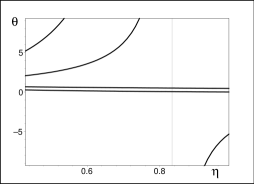
The spectrum of energies may be then easily calculated and found sampled in Fig. 1. The parameter-dependence of the energies seems to be such that they avoid “collisions”. As long as we choose $\lambda=1$, i.e., Hamiltonian

$$\mathfrak{h}^{(\epsilon,1)}=\left[\begin{array}[]{cccc}0&-1+i\epsilon&0&0\\ \vskip 6.0pt plus 2.0pt minus 2.0pt\cr-1-i\epsilon&0&-1+i\epsilon&0\\ \vskip 6.0pt plus 2.0pt minus 2.0pt\cr 0&-1-i\epsilon&0&-1+i\epsilon\\ \vskip 6.0pt plus 2.0pt minus 2.0pt\cr 0&0&-1-i\epsilon&0\end{array}\right]$$ (14)

the quadruplet of the energy eigenvalues becomes available also in the closed form

$$E_{\pm,\pm}=\pm\frac{1}{2}\,\sqrt{\left(6\pm 2\,\sqrt{5}\right)\left(1+{\epsilon}^{2}\right)}\,.$$ (15)

This formula explains not only the hyperbolic shapes of the curves in Fig. 1 but also their closest-approach values $E_{\pm,+}\approx\pm 1.618033988$ and $E_{\pm,-}\approx\pm 0.6180339880$ at $\epsilon=0$.

The details of the generic avoided-crossing phenomenon are model-dependent but an analogous observation will be made using any  Hermitian-matrix Hamiltonian. The explanation may be found in the Kato’s book [27]. In essence, the Kato’s mathematical statement is that once a given matrix is self-adjoint alias Hermitian, then in the generic case (i.e., without any additional symmetries) an arbitrary pair of the eigenvalues can only merge at the so called exceptional-point (EP) value of the parameter. In the Hermitian diagonalizable (i.e., physical) cases these EP values are all necessarily complex so that whenever the parameter remains real, the distances between the separate real eigenvalues behave as if controlled by a mutual “repulsion” [28]. From Fig. 1 we may then extract one of the key messages mediated by the model, viz., the observation that the unitary evolution is “robust”. One may expect that whenever we need to achieve an unavoided crossing of the eigenvalues, the more adequate description of the phenomenon will be provided by the transition to non-Hermitian Hamiltonians in ${\cal F}^{(NH)}$ for which the EP values may be real.

4 Attraction of eigenvalues

The phenomenon of the existence of a minimal distance between the energy levels of a Hermitian matrix is generic. After one tries to move from family ${\cal F}^{(H)}$ to family ${\cal F}^{(NH)}$, the robust nature of such an obstruction is lost. The reason lies in the above-mentioned change of the geometry of the Hilbert spaces in question. The resulting new freedom of models in ${\cal F}^{(NH)}$ may find applications, e.g., in an effective description of non-unitarities in open quantum systems [29] or, in cosmology, in an elementary explanation of the possibility of a consistently quantized Big Bang [30].

4.1 Local interactions

One of the reasons of the recent turn of attention to the hiddenly Hermitian local-interaction models (cf. their sample (10) above) is that the mapping $H\to\mathfrak{h}$ of Eq. (5) produces, in general, strongly nonlocal generalizations of the conventional local Hamiltonians (6). The same argument works in both directions and it enriched the scope of the conventional quantum theory [3, 4]. Several impressive constructive illustrations of such a type of enrichment of the class of the tractable quantum models (treating the direct use of local-interaction models (7) as an important extension of the applied quantum theory) may be found, e.g., in Ref. [25]. One may conclude that the local-interaction nature and constructive tractability of the alternative models (10) contained in class ${\cal F}^{(NH)}$ would render their isospectral partners (3) non-local. Thus, some of the weaker forms of the nonlocalities as sampled, e.g., in Refs. [17, 22] may be expected necessary for the constructive search for the non-empty interfaces ${\cal F}^{(H)}\bigcap{\cal F}^{(NH)}$.

4.2 Weakly non-local interactions

For the purposes of the most elementary though still sufficiently rich illustration of some technical aspects of the transition from ${\cal F}^{(H)}$ to ${\cal F}^{(NH)}$ one may perform the straightforward de-Hermitization of Eq. (13). This yields the two-parametric pencil of Hamiltonian matrices

$$H^{(\eta,\lambda)}=T+\eta\,W^{(\lambda)}=\left[\begin{array}[]{cccc}0&-1+\eta&0&0\\ \vskip 6.0pt plus 2.0pt minus 2.0pt\cr-1-\eta&0&-1+\eta\,\lambda&0\\ \vskip 6.0pt plus 2.0pt minus 2.0pt\cr 0&-1-\eta\,\lambda&0&-1+\eta\\ \vskip 6.0pt plus 2.0pt minus 2.0pt\cr 0&0&-1-\eta&0\end{array}\right]\neq\left[H^{(\eta,\lambda)}\right]^{\dagger}\,$$ (16)

characterized by a minimal, tridiagonal-matrix non-locality of their interaction component. For real $\eta$ and $\lambda$ the related energy spectra only remain real (i.e., observable and phenomenologically meaningful) in certain physical parametric intervals.

Figure 2: The attraction (followed by the loss of reality) in the case of the eigenvalues of the manifestly non-Hermitian matrix (16) at $\lambda=6/5$.

The simplicity of our toy model (16) enables us to illustrate the latter statement by recalling the explicit formula for the eigenvalues,

$$E_{(\pm,\pm)}(\epsilon,\lambda)=\pm\frac{1}{\sqrt{2}}\,\sqrt{3-\left({\lambda}^{2}+2\right)\,{\epsilon}^{2}\pm\sqrt{\left[5-\left({\lambda}^{2}+4\right)\,{\epsilon}^{2}\right]\left(1-\lambda^{2}\,\epsilon^{2}\right)}}\,\ .$$ (17)

The knowledge of this formula enables us to separate the interval of the interaction-controlling parameters $\lambda$ into three qualitatively different subintervals.

4.2.1 $\lambda>1$ (strong non-Hermiticities)

The first, $\lambda>1$ sample of the energy spectrum is displayed here in Fig. 2. The picture shows that at the two real exceptional points $\eta=\eta^{(EP)}$ such that $|\eta|=|\eta^{(EP)}|<1$ the (real-energy) quadruplets of energies degenerate and, subsequently, acquire imaginary components. These complexifications proceed pairwise, i.e., our four-level model effectively decays into two almost independent, weakly coupled two-level systems. The full descriptive wealth of our model will only manifest itself at the smaller values of $\lambda$.

Figure 3: Same as Fig. 2, with smaller $\lambda=3/5$.

4.2.2 $\lambda<1$ (weak non-Hermiticities)

In Fig. 3 using a smaller $\lambda<1$ a much more interesting scenario is displayed in which all of the four energy levels are mutually attracted. Firstly we notice that the complexifications of the eigenvalues occur at the EP values $\eta^{(EP)}_{(first\ kind)}$ which are “large”, i.e., such that $|\eta^{(EP)}_{(first\ kind)}|>1$. The domain of the observability of the energies is larger than interval $(-1,1)$. Still, the latter interval has natural boundaries because of the emergence of the other two EP degeneracies at $\eta^{(EP)}_{(second\ kind)}=\pm 1$. These new singularities are characterized by the unavoided level crossings without a complexification. Their occurrence splits the interval of $\eta$ into separate subintervals. The consequences for the quantum phenomenology are remarkable, e.g., for the reasons which were discussed, recently, in [11]

Figure 4: The confluence of exceptional points at $\lambda=1$.

4.2.3 $\lambda=1$ (the instant of degeneracy)

The shared boundary between the two dynamical regimes is characterized by Fig. 4. The algebraic representation of the $\lambda=1$ spectrum is elementary,

$$E_{\pm,\pm}=\pm\frac{1}{2}\,\sqrt{\left(6\pm 2\,\sqrt{5}\right)\left(1-{\eta}^{2}\right)}\,.$$ (18)

The formula may be read as an analytic continuation of Eq. (15).

5 The model with interface

5.1 Hilbert-space metric

In comparison with the conventional textbook family ${\cal F}^{(H)}$, the practical use of the non-Hermitian phenomenological Hamiltonians in ${\cal F}^{(NH)}$ is certainly much more difficult. One of the key complications is to be seen in the (in general, non-unique) reconstruction of the metric from the given observables or, in the simplest case, from Hamiltonian $H$.

The ambiguity of the reconstruction may be illustrated by the insertion of our two-parametric toy-model $N=4$ Hamiltonian $X=H^{(\eta,\lambda)}$ of Eq. (16) in the quasi-Hermiticity constraint (28) in Appendix A interpreted as an implicit definition of $\Theta^{(\eta,\lambda)}=\Theta(H^{(\eta,\lambda)})$. After a tedious but straightforward algebra one obtains the general result

$$\Theta^{(\eta,\lambda)}_{(c,d,f,g)}=\left[\begin{array}[]{cccc}{\it A}(f,c)&{\frac{\left(g-d\right)\left(1+\eta\right)}{1-\eta\,\lambda}}&{\frac{{\it{c}}}{1-\eta}}&d\\ \vskip 6.0pt plus 2.0pt minus 2.0pt\cr{\frac{\left(g-d\right)\left(1+\eta\right)}{1-\eta\,\lambda}}&{\frac{{\it{f}}}{1-\eta\,\lambda}}&g&{\frac{{\it{c}}}{1+\eta}}\\ \vskip 6.0pt plus 2.0pt minus 2.0pt\cr{\frac{{\it{c}}}{1-\eta}}&g&{\frac{{\it{f}}}{1+\eta\,\lambda}}&{\frac{\left(g-d\right)\left(1-\eta\right)}{1+\eta\,\lambda}}\\ \vskip 6.0pt plus 2.0pt minus 2.0pt\cr d&{\frac{{\it{c}}}{1+\eta}}&{\frac{\left(g-d\right)\left(1-\eta\right)}{1+\eta\,\lambda}}&{\it F}(f,c)\end{array}\right]$$ (19)

where

$${\it A}(f,c)={\frac{{\it{f}}-{\it{f}}\,{\eta}^{2}-{\it{c}}+{\it{c}}\,{\eta}^{2}{\lambda}^{2}}{\left(1-\eta\right)^{2}\left(1-\eta\,\lambda\right)}}$$ (20)

and

$${\it C}(f,c)={\frac{{\it{f}}-{\it{f}}\,{\eta}^{2}-{\it{c}}+{\it{c}}\,{\eta}^{2}{\lambda}^{2}}{\left(1+\eta\right)^{2}\left(1+\eta\,\lambda\right)}}\,.$$ (21)

Thus, one can summarize that unless we add more requirements, the specification of the mere Hamiltonian leads to the four-parametric family of the inner-product metric-operators (19). Obviously, this opens the possibility of the choice of the additional observables which would have to satisfy Eq. (28) and, thereby, restrict the freedom in our choice of the parameters $c,d,f$ and $g$.

One of the possible formal definitions of an “interface” between the alternative descriptions (2) and (4) of a quantum system may be based on the presence of a variable parameter or parameters (say, of a real $\sigma\in(-\infty,\infty)$) such that $\mathfrak{h}=\mathfrak{h}(\sigma)$ and $H=H(\sigma)$. One may then reveal that there exists a point $\sigma_{0}$ or a non-empty closed vicinity $I_{0}=(\sigma_{-},\sigma_{+})$ of this point such that the formally equivalent Schrödinger Eqs. (2) and (4) are also more or less equally user-friendly when $\sigma\in I_{0}$. Naturally, such a concept will make sense when just the solution of one of the Schrödinger equations remains feasible and practically useful far from $\sigma_{0}$.

Whenever one tries to treat $\sigma$ as a function of time, a number of technical complications immediately emerges (the most recent account of some of them may be found in [31]). One has to assume, therefore, that the time-variation of $\sigma$ as well as the $\sigma-$variation of the Hamiltonians remains sufficiently slow, i.e., so slow that the corresponding time-derivatives of $\sigma$ and the $\sigma-$derivatives of the Hamiltonians remain negligible. Under these assumptions, the passage of certain quantum systems through their respective HSP - NHSP interfaces can be shown possible.

5.2 Illustrative Hamiltonian

One of the most straightforward implementations of the above idea may be based on the identification of the above-introduced parameter $\sigma$ with the parameter $\epsilon$ of Eq. (12) (and, say, of Fig. 1) along the negative real half-axis, and with the parameter $\eta$ of Eq. (16) (and of Fig. 4) along the positive real half-axis. In such an arrangement the interval of a large and negative $\sigma\ll-1$ will be the domain in which the use of the non-Hermitian picture ${\cal F}^{(NH)}$ (with any nontrivial metric) would prove absolutely useless. In parallel, any attempt of working with the Hermitian picture ${\cal F}^{(H)}$ will necessarily fail close to $\sigma\approx+1$ and further to the right. At the same time, in practically any interval of the positive $\sigma=\eta\in I_{0}=(0,\sigma_{+})$ with $\sigma_{+}<1$ we would be able to work, more or less equally easily, with both of the non-Hermitian and Hermitian versions of the matrix.

The main advantage of the work in simultaneous pictures, i.e., with the Hamiltonian matrix defined in ${\cal F}^{(interface)}$ may be seen in the smoothness of the transitions to both of the neighboring pictures ${\cal F}^{(H)}$ and ${\cal F}^{(NH)}$. This smoothness is nontrivial because the respective behaviors of the quantum system in question will be different, in spite of the unified definition of the dynamics. Thus, once we set

$$H^{(unified)}=\left[\begin{array}[]{cccc}0&-1+\gamma(\tau)&0&0\\ \vskip 6.0pt plus 2.0pt minus 2.0pt\cr-1-\gamma(\tau)&0&-1+\gamma(\tau)&0\\ \vskip 6.0pt plus 2.0pt minus 2.0pt\cr 0&-1-\gamma(\tau)&0&-1+\gamma(\tau)\\ \vskip 6.0pt plus 2.0pt minus 2.0pt\cr 0&0&-1-\gamma(\tau)&0\end{array}\right]$$ (22)

with

$$\gamma(\tau)=\sqrt{\tau^{2}\cdot{\rm sign}\ \tau}=\sqrt{\tau\cdot|\tau|}=\left\{\begin{array}[]{ll}{\rm i}\tau\,,&\tau<0\,,\\ \tau\,,&\tau\geq 0\end{array}\right.$$ (23)

we will be able to interpolate, smoothly, between the eigenvalue repulsion to the left and the eigenvalue attraction to the right (see Fig. 5).

Figure 5: Monotonic convergence of eigenvalues of matrix (22) with the growth of $\tau$.

In addition, one may also appreciate the asymmetry of the spectrum. In the purely phenomenological setting it could be interpreted, e.g., as a transition from the conventional and robust dynamical regime to the emergence of an instability and collapse at positive $\tau=1$. Marginally, let us also note that our choice of notation is indicative because $\tau$ might have been perceived as a time variable, in an adiabatic regime at least [31]. Another marginal comment is that at $\tau>\tau^{(EP)}=1$, i.e., at $\tau=\sqrt{1+\varrho^{2}}>1$, the eigenvalues form the two purely imaginary complex-conjugate pairs

$$\pm\frac{{\rm i}\varrho}{2}\,\sqrt{\left(6\pm 2\,\sqrt{5}\right)}\approx\left\{\begin{array}[]{ll}\pm 1.618033988\ {\rm i}\varrho\\ \pm 0.6180339880\ {\rm i}\varrho\end{array}\right.\,.$$ (24)

Figure 6: Same as Fig. 5 but with a slightly smaller $\lambda=3/5$.

In the light of our preceding analysis it is not too surprising that for the larger values of $\lambda>1$ the simultaneous complexification of the eigenvalues would occur at a slightly smaller EP singularity $\tau^{(EP)}<1$ and that the model would effectively decay into the two two-level subsystems. Such an observation might be contrasted with the more interesting spectral pattern obtained at $\lambda=3/5$ and displayed in Fig. 6.

5.3 The interface-compatible metrics

The physical interpretation of the parameter $\sigma$ need not be specified at all. Its interface values $\sigma_{0}\in I_{0}$ might mark a critical time or the position of a spatial boundary or a critical value of the strength of influence of an environment, etc.

In our present illustrative model the specification of the left boundary point $\sigma_{-}=0$ is unique because of the natural choice of $\Theta=I$ along the whole negative half-axis of $\sigma$. In contrast, our choice of the right boundary point $\sigma_{+}<1$ remains variable because we always have $\Theta\neq I$ for all of the positive physical values of $\sigma$.

We have to match the Hermitian choice of $\Theta=I$ valid at the negative half-axis of $\sigma\leq 0$ to the hidden-Hermiticity choice of $\Theta\neq I$ at the small and positive $\sigma>0$. We may recall formula (19) and deduce that

$$\lim_{\eta\to 0}\,\Theta^{(\eta,\lambda)}_{(c,d,f,g)}=\left[\begin{array}[]{cccc}{\it{f}}-{\it c}&g-d&{\it c}&d\\ \vskip 6.0pt plus 2.0pt minus 2.0pt\cr g-d&{\it{f}}&g&{\it c}\\ \vskip 6.0pt plus 2.0pt minus 2.0pt\cr{\it c}&g&{\it{f}}&g-d\\ \vskip 6.0pt plus 2.0pt minus 2.0pt\cr d&{\it c}&g-d&{\it{f}}-{\it c}\end{array}\right]\,.$$ (25)

Even if we admit that the values of the parameters in the metric may be $\eta-$dependent, $c=c(\eta),d=d(\eta),f=f(\eta)$ and $g=g(\eta)$, we must demand that $d(0)=c(0)=g(0)=0$ and normalize, say, $f(0)=1$. This yields the metric which is diagonal at $\eta=0$ and which remains diagonal after we require that the parameters remain constant, $\eta-$independent. The elements forming the diagonal of such a special Hilbert-space metric $\Theta$ read

$$\left\{\frac{1+\eta}{(1-\eta)(1-\eta\lambda)},\frac{1}{1-\eta\lambda},\frac{1}{1+\eta\lambda},\frac{1-\eta}{(1+\eta)(1+\eta\lambda)}\right\}\ .$$ (26)

In Fig. 7 we may see the coincidence of these elements in the limit $\eta\to 0$, demonstrating the smooth variation of the metric $\Theta$ in the both-sided vicinity of $\eta=0$.

Figure 7: The $\eta-$dependence of the eigenvalues of the metric $\Theta$ of Eq. (26) at $\lambda=6/5$.

The construction of the kinetic-energy part $T$ of all of our toy model matrix Hamiltonians $H$ with $N=4$ was based on the assumption that there exist coordinates $q$ forming a spatial grid-point lattice. In the present context this means that once the metric (26) remains diagonal, in an interval of small $\sigma=\eta>0$ at least, we may conclude that the strong-non-locality effects as caused by the metric $\Theta$ and observed, say, in Refs. [16, 25] are absent here. In this sense, our present model shares the weak-nonlocality merits of its predecessors in Refs. [17, 22].

Figure 8: The prolongation of Fig. 7 beyond $\eta^{(EP)}=5/6$.

Our diagonal metric remains positive and invertible, at the sufficiently small $\eta$ at least. Naturally, it also has the EP-related singularities at $\eta^{(EP)}_{(first\ kind)}=\pm 1/\lambda$. Their occurrence and $\lambda-$dependence is illustrated here in Fig. 8. Naturally, for $\lambda<1$ there emerge also the singularities at $\eta^{(EP)}_{(second\ kind)}=\pm 1$ (see the dedicated Ref. [11] for a more thorough explanation of this terminology).

6 Summary and conclusions

In the conventional applications to quantum theory, the description of the unitary evolution of a given system ${\cal S}$ need not necessarily be performed in Schrödinger picture (cf., e.g., the compact review of its eight eligible alternatives in [18]). Naturally, once people decide to prefer the work in Schrödinger picture, they usually recall the Stone’s theorem [23] and conclude that the Hamiltonian (i.e., in our present notation, operator $\mathfrak{h}\in{\cal F}^{(H)}$ acting in the conventional Hilbert space ${\cal H}^{(textbook)}$) must necessarily be Hermitian (for the sake of brevity we spoke here about the HSP realization of Schrödinger picture).

Along a complementary, different line of thinking which dates back to Dyson [1] and which recently climaxed with Bender [4] and Mostafazadeh [3], the community of physicists already accepted the consistency of the alternative, NHSP realization of the same Schrödinger picture. In the NHSP version and language the Hamiltonian (i.e., the upper-case operator $H\in{\cal F}^{(NH)}$ with real spectrum) is naturally self-adjoint in the physical Hilbert space ${\cal H}^{(redefined)}$ which is, unfortunately, highly unconventional. The same operator $H$ only appears  manifestly non-Hermitian in the other, auxiliary, “redundant” Hilbert space ${\cal H}^{(unphysical)}$ which is, by assumption, “the friendliest” one.

It is unfortunate that the latter, historically developed terminology is so confusing. This is one of the explanations why the methodically important question of the possible HSP/NHSP overlap of applicability has not yet been properly addressed and clarified in the literature. In our present paper we filled the gap by showing that such an overlap (called, by Jones [16], an “interface”) may exist. We also emphasized that the construction of the interface should start from the upper-case (and, typically, one-parametric) family of the hiddenly Hermitian NHSP Hamiltonians operators $H=H(\sigma)\in{\cal F}^{(NH)}$ and that it has to be based on the analysis of the related family of the Hermitizing metric operators $\Theta=\Theta[H(\sigma)]$.

In such a framework one can conclude that Hamiltonian $H=H(\sigma)$ with $\sigma\in(\sigma_{-},\sigma_{+})$ can be perceived as an element of an HSP/NHSP overlap ${\cal F}^{(interface)}\neq\emptyset$, provided only that the Hermitizing metric operator at our disposal (i.e., operator $\Theta=\Theta[H(\sigma)]$) is such that

$$\lim_{\sigma\to\sigma_{-}}\Theta[H(\sigma)]=I\,.$$ (27)

In other words, once we have $H(\sigma_{-})=H^{\dagger}(\sigma_{-})$, we may now introduce the quantum Hamiltonians $\mathfrak{h}(\sigma)$ (which lie, by construction, in ${\cal F}^{(H)}$) in such a way that they are connected with $H(\sigma)$ (i.e., defined) by relation (5) at $\sigma\in(\sigma_{-},\sigma_{+})$ while their definition may be continued to $\sigma<\sigma_{-}$ arbitrarily (e.g., by the most straightforward constant-operator prescription $\mathfrak{h}(\sigma)=H(\sigma_{-})$).

The lower boundary $\sigma_{-}0$ of the interval of the interface-compatible parameters carries an immediate physical meaning of a point of transition from the HSP eigenvalue repulsion regime (guaranteeing the robust reality of the spectrum) to the NHSP eigenvalue attraction (and, possibly, complexification). Via na elementary illustrative example we demonstrated that the resulting “mixed” dynamics could enrich the current phenomenological considerations in quantum theory. Naturally, this is a task for future research because our present, methodically motivated and analytically solvable example is only too schematic for such a purpose.

Appendix A. Unitary evolution via non-Hermitian $H$

A. 1. The third Hilbert space

Strictly speaking, the real spectra of eigenvalues of $H\neq H^{\dagger}$ as well as of any other operator $X\neq X^{\dagger}$ of the observable characterizing the quantum system in question cannot be assigned any immediate physical meaning because the underlying Hilbert space ${\cal H}^{(unphysical)}$ is, by definition, just auxiliary and “incorrect”. The “correct” meaning of the observables can only be established in the “correct” Hilbert space ${\cal H}^{(textbook)}$. Whenever needed, any experimental prediction may be reconstructed using the correspondences $\psi(t)=\Omega\,\Psi(t)$, $\mathfrak{h}=\Omega\,H\,\Omega^{-1}\,$ and $\mathfrak{x}=\Omega\,X\,\Omega^{-1}\,$.

One of the benefits of the NHSP representation is that in the generic stationary case the full knowledge of the Dyson’s operator $\Omega$ is not necessary. What controls the predictions are just the mean values of the operators of observables. For them, the translations of the relevant formulae from ${\cal H}^{(textbook)}$ to ${\cal H}^{(unphysical)}$ may be shown to contain only the so called Hilbert-space metric, i.e., the Dyson-map product $\Theta=\Omega^{\dagger}\Omega$ (see, e.g., [2] for more details). This implies that in a close parallel to Eq. (5), all of the observables of a system in question may be represented by the diagonalizable operators $X\neq X^{\dagger}$ with real spectra which only have to satisfy the generalized Hermiticity relation

$$X^{\dagger}\Theta=\Theta\,X\,.$$ (28)

Any Hilbert space metric $\Theta$ which is “mathematically acceptable” (see [3] for details) may be interpreted as redefining the inner product in ${\cal H}^{(unphysical)}$. This redefinition of the inner product may be re-read as a redefinition of the Hilbert space itself,

$${\cal H}^{(unphysical)}\to{\cal H}^{(redefined)}\,.$$ (29)

By construction, the new space becomes unitarily equivalent to ${\cal H}^{(textbook)}$. This means that we may re-interpret Hamiltonians $H$ (sampled by Eq. (10) and non-Hermitian in auxiliary ${\cal H}^{(unphysical)}$) as self-adjoint in the new Hilbert space ${\cal H}^{(redefined)}$. Thus, using the notation of Ref. [20] we may write $H=H^{\ddagger}$, with the definition of $H^{\ddagger}=\Theta^{-1}H^{\dagger}\Theta$ being deduced from Eq. (5) above.

In opposite direction our quantum-model-building may start from a given $N-$plet $\{X_{n}\}$ of candidates for the observables. As long as all of these operators (defined in ${\cal H}^{(unphysical)}$) must satisfy the respective hidden Hermiticity condition (28), there must exist a metric candidate $\Theta=\Theta(X_{1},\ldots,X_{N})$ compatible with all of these hidden-Hermiticity conditions. Thus, the metric need not exist at all (see an example in [32]). If it does exist, it may be either ambiguous (see an example in [25]) or unique (see, e.g., a large number of examples in [4]).

A. 2. Physical inner products

The non-Hermiticity property of operators might cause complications in calculations. Also the assumptions of the user-friendliness of ${\cal H}^{(unphysical)}$ and/or of $H(t)$ seem highly nontrivial. On the level of theory one must keep in mind that the new, friendlier Hilbert space is, by itself, merely auxiliary and unphysical. In principle, a return to ${\cal H}^{(textbook)}$ is needed whenever experiment-related predictions are asked for. Still, whenever the structure of such a space and/or of the observables (defined in this space and sampled by Hamiltonian $\mathfrak{h}$) appear prohibitively complicated, the evaluation of the predictions of the theory is to be made also directly in ${\cal H}^{(unphysical)}$. Due care must only be paid to the insertions of the metric operator $\Theta=\Omega^{\dagger}\Omega\neq I$ (i.e., to the amendments of the inner products) whenever applicable [3].

Figure 9: The three-Hilbert-space representation pattern.

People do not always notice that after the latter amendment of the inner product our auxiliary Hilbert space ${\cal H}^{(unphysical)}$ becomes redefined and converted into another, third Hilbert space ${\cal H}^{(redefined)}$ which is, by construction, physical, i.e., unitarily equivalent to ${\cal H}^{(textbook)}$. Thus, whenever we start from Eq. (4), the quantum system in question becomes simultaneously  represented in a triplet  of Hilbert spaces (the pattern is displayed in Fig. 9).

Naturally, the Stone’s theorem does not get violated due to the one-to-one, $\Omega-$mediated correspondence between $H$ and $\mathfrak{h}$. Due to the property $\Omega^{\dagger}\Omega=\Theta\neq I$ of the Dyson’s non-unitary mappings, the Hermiticity of the conventional Hamiltonian $\mathfrak{h}$ in the physical space ${\cal H}^{(textbook)}$ becomes replaced, in the auxiliary and manifestly unphysical Hilbert space ${\cal H}^{(unphysical)}$, by the hidden Hermiticity alias $\Theta-$pseudo-Hermiticity [3] property $H=\Theta^{-1}H^{\dagger}\Theta\$ of the upper-case non-Hermitian Hamiltonian with real spectrum (cf. Eq. (4) above). In the related literature one can also read about the closely related concepts of quasi-Hermiticity (see [2]), unbroken ${\cal PT}-$symmetry [4] or crypto-Hermiticity [20, 33] of $H$ and/or, last but not least, about the quasi-similarity between $H$ and $H^{\dagger}$ [34].

A. 3. The Hermitian-theory point of view

Technically, it is usually easier to work with the elements of the “Hermitian” family ${\cal F}^{(H)}$ comprising the traditional quantum systems and the traditional textbook self-adjoint Hamiltonians $\mathfrak{h}=\mathfrak{h}^{\dagger}$. Dyson [1] merely proposed that sometimes, it may still make sense to make use of the other, innovative family ${\cal F}^{(NH)}$ which works with the “non-Hermitian” Schrödinger Eqs. (4). Certainly, the latter family is not small. Pars pro toto  it contains Hamiltonians of relativistic quantum mechanics [35, 36], the well known ${\cal PT}-$symmetric imaginary cubic oscillator [37, 38] (which appears, after a more detailed scrutiny, strongly non-local [25, 39]), its power-law generalizations [10, 40] as well as exactly solvable models [41], models with methodical relevance in the context of supersymmetry [42], realistic and computation-friendly interacting-boson models of heavy nuclei [2], benchmark candidates for classification of quantum catastrophes [43], etc.

In the majority of the above-listed models defined in ${\cal F}^{(NH)}$ one may still keep in mind that their physical contents can always be sought in their equivalence to the partner Hamiltonians (and/or other observables) in ${\cal F}^{(H)}$. Thus, the use of the less usual representation in ${\cal F}^{(NH)}$ is treated as a mere technical trick.

The main argument against the latter, fairly widespread point of view may be formulated as an objection against the over-intimate, history-produced relationship between the way of our thinking in classical physics and the related production of the “conventional” quantum models in ${\cal F}^{(H)}$ by the techniques of the so called “quantization”. In principle, we should have been much more humble, taking rather the classical world as a result of making its quantum picture “de-quantized” [44].

References

- [1] F. J. Dyson, Phys Rev 102, 1217 (1956).
- [2] F. G. Scholtz, H. B. Geyer and F. J. W. Hahne, Ann. Phys. (NY) 213, 74 (1992).
- [3] A. Mostafazadeh, Int. J. Geom. Meth. Mod. Phys. 7, 1191 (2010).
- [4] C. M. Bender, Rep. Prog. Phys. 70, 947 (2007).
- [5] J. Dieudonné, in Proc. Int. Symp. Lin. Spaces. Oxford, Pergamon, 1961, p. 115.
- [6] J. Alexandre, C. M. Bender and P. Millington, J. High Energy Phys. 11, 111 (2015).
- [7] J. Alexandre, C. M. Bender, and P. Millington J. Phys.: Conf. Ser. 873, 012047 (2017).
- [8] T. J. Milburn, J. Doppler, C. A. Holmes, S. Portolan, S. Rotter and P. Rabl, Phys. Rev. A 92, 052124 (2015).
- [9] A. Mostafazadeh, Phys. Lett. B 650, 208 (2007).
- [10] C. M. Bender and S. Boettcher, Phys. Rev. Lett. 80, 5243 (1998); C. M. Bender, D. C. Brody and H. F. Jones, Phys. Rev. Lett. 89, 270401 (2002) and ibid. 92 119902 (2004) (erratum).
- [11] D. I. Borisov, Acta Polytechnica 54, 93 (2014) (arXiv:1401.6316); D. I. Borisov, F. Růžička and M. Znojil, Int. J. Theor. Phys. 54, 4293 (2015); M. Znojil, Ann. Phys. (NY) 336, 98 (2013); D.I. Borisov and M. Znojil, in “Non-Hermitian Hamiltonians in Quantum Physics”, F. Bagarello, R. Passante and C. Trapani, eds. (Springer, 2016), pp. 201-217.
- [12] C. E. Rüter, K. G. Makris, R. El-Ganainy, et al., Nat. Phys. 6, 192 (2010).
- [13] F Bagarello, J-P Gazeau, F H Szafraniec and M Znojil, editors, Non-Selfadjoint Operators in Quantum Physics: Mathematical Aspects. John Wiley & Sons, Hoboken, 2015.
- [14] M. Znojil, Phys. Rev. D. 80, 045009 (2009).
- [15] H. F. Jones, Phys. Rev. D 76, 125003 (2007)
- [16] H. F. Jones, Phys. Rev. D 78, 065032 (2008).
- [17] M. Znojil, J. Phys. A: Math. Theor. 41, 292002 (2008); M. Znojil, Symm. Integr. Geom. Methods Appl. (SIGMA) 5, 085 (2009).
- [18] D. F. Styer et al, Am. J. Phys. 70, 288 (2002).
- [19] A. Messiah, Quantum Mechanics I. North Holland, Amsterdam, 1961.
- [20] M. Znojil, SIGMA 5, 001 (2009) (e-print overlay: arXiv:0901.0700).
- [21] H. F. Jones, 6th Int. Workshop PHHQP (2007), talk and transparencies on web: http://www.staff.city.ac.uk/fring/PT/Timetable.html# jones
- [22] M. Znojil, Phys. Rev. D 78 (2008) 025026.
- [23] M. H. Stone, Ann. Math. 33, 643 (1932).
- [24] S. Flügge, Practical Quantum Mechanics II. Springer, Berlin, 1971.
- [25] A. Mostafazadeh, J. Phys. A: Math. Gen. 39, 10171 (2006).
- [26] M. Znojil, Phys. Rev. A 96, 012127 (2017).
- [27] T. Kato, Perturbation theory for linear operators, Springe, Berlin, 1966.
- [28] A deeper analysis may be found in the Kato’s book [27].
- [29] U. Günther and B. F. Samsonov, Phys. Rev. Lett. 101, 230404 (2008).
- [30] M. Znojil, J. Phys. Conf. Ser. 343, 012136 (2012); M. Znojil, in F. Bagarello, R. Passante and C. Trapani, eds, Non-Hermitian Hamiltonians in Quantum Physics. Springer, Cham, 2016, pp. 383 - 399.
- [31] M. Znojil, Ann. Phys. (NY) 385, 162 (2017).
- [32] M. Znojil, I. Semorádová, F. Růžička, H. Moulla and I. Leghrib, Phys. Rev. A 95, 042122 (2017).
- [33] A. V. Smilga, J. Phys. A: Math. Theor. 41, 244026 (2008).
- [34] J.-P. Antoine and C. Trapani, in [13], pp. 345 - 402.
- [35] A. Mostafazadeh, Ann. Phys. (N.Y.) 309, 1 (2004).
- [36] V. Jakubský and J. Smejkal, Czech. J. Phys. 56, 985 (2006).
- [37] E. Caliceti, S. Graffi and M. Maioli, Commun. Math. Phys. 75, 51 (1980); G. Alvarez, J. Phys. A: Math. Gen. 27, 4589 (1995).
- [38] D. Bessis, private communication (1992); G. Alvarez, private communication (1994).
- [39] P. Siegl and D. Krejčiřík, Phys. Rev. D 86, 121702(R) (2012).
- [40] M. Znojil, Phys. Lett. A 374, 807 (2010).
- [41] M. Znojil, Phys. Lett. A 259, 220 (1999); G. Lévai and M. Znojil, J. Phys. A: Math. Gen. 33, 7165 (2000); M. Znojil, Phys. Lett. A 285, 7 (2001); M. Znojil and G. Lévai, Mod. Phys. Lett. A 16, 2273 (2001).
- [42] B. Bagchi, Supersymmetry in Quantum and Classical Mechanics. Chapman and Hall/CRC, 2000; M Znojil, J. Phys. A: Math. Gen. 35, 2341 (2002).
- [43] M. Znojil, J. Phys. A: Math. Theor. 40, 4863 (2007) and 40, 13131 (2007); M. Znojil, J. Phys. A: Math. Theor. 45, 444036 (2012).
- [44] D. C. Brody and L. P. Hughston, J. Geom. Phys. 38, 19 (2001).