Separating cycles and isoperimetric
inequalities in the uniform infinite
planar quadrangulation

Abstract

We study geometric properties of the infinite random lattice called the uniform infinite planar quadrangulation or UIPQ. We establish a precise form of a conjecture of Krikun stating that the minimal size of a cycle that separates the ball of radius $R$ centered at the root vertex from infinity grows linearly in $R$. As a consequence, we derive certain isoperimetric bounds showing that the boundary size of any simply connected set $A$ consisting of a finite union of faces of the UIPQ and containing the root vertex is bounded below by a (random) constant times $|A|^{1/4}(\log|A|)^{-(3/4)-\delta}$, where the volume $|A|$ is the number of faces in $A$.

T1Supported by the ERC Advanced Grant 740943 GeoBrown

and

1 Introduction

In the recent years, much work has been devoted to discrete and continuous models of random geometry in two dimensions. Two of the most popular discrete models are the uniform infinite planar triangulation (or UIPT), which was introduced by Angel and Schramm [1, 2] and in fact motivated much of the subsequent work, and the uniform infinite planar quadrangulation (or UIPQ). In the present work, we concentrate on the UIPQ, although we believe that our methods can be adapted to give similar results for the UIPT. Roughly speaking, the UIPQ is a random infinite graph embedded in the plane, such that all faces (connected components of the complement of edges) are quadrangles, possibly with two edges glued together. See Fig.4 below for an illustration of what the UIPQ may look like near its root vertex. We study certain geometric properties of the UIPQ, concerning the existence of “small” cycles that separate a large ball centered at the root vertex from infinity, with applications to isoperimetric inequalities.

The starting point of our work is a conjecture of Krikun in the paper [14] which provided the first construction of the UIPQ as the local limit of uniform planar quadrangulations with a fixed number of faces (another construction was suggested by Chassaing and Durhuus [3], and the equivalence between the two approaches was established by Ménard [18] — see also [9] for a third construction). Denote the UIPQ by ${\mathcal{P}}$, and, for every integer $r\geq 1$, let $B_{r}({\mathcal{P}})$ stand for the ball of radius $r$ centered at the root vertex, which is defined as the union of all faces that are incident to at least one vertex whose graph distance from the root is at most $r-1$. The complement of the ball $B_{r}({\mathcal{P}})$ is in general not connected, but there is a unique unbounded component, whose boundary is called the exterior boundary of the ball. The set inside the exterior boundary, which may be obtained by filling in the “bounded holes” of the ball, is called the (standard) hull of radius $r$ and will be denoted by $B^{\bullet}_{r}({\mathcal{P}})$. It is known that the size of the exterior boundary, that is, the number of edges in this boundary, grows like $r^{2}$ when $r\to\infty$: See [7] for more precise asymptotics obtained both for the UIPT and the UIPQ. On the other hand, Krikun constructed a cycle that separates the ball $B_{r}({\mathcal{P}})$ from infinity and whose size grows linearly in $r$ when $r$ is large. Here we say that a cycle $\mathcal{C}$ made of edges of the UIPQ separates a finite set $A$ of vertices from infinity if $A$ does not intersect $\mathcal{C}$ but any path from a vertex of $A$ to infinity intersects $\mathcal{C}$ (see Fig. 1 for a schematic illustration). Krikun conjectured that the cycle he constructed is essentially the shortest possible, meaning that the minimal size of a cycle that separates the ball $B_{r}({\mathcal{P}})$ from infinity must be linear in $r$. A weak form of this conjecture was derived in [5], but the results of this paper did not exclude the possibility that a ball could be separated from infinity by a small cycle lying “very far away” from the ball.

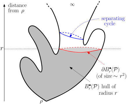
Figure 1: A schematic “cactus” representation of the UIPQ. The root vertex is denoted by $\rho$ and the vertical coordinate corresponds to the graph distance from $\rho$. The shaded part is the hull $B^{\bullet}_{r}(\mathcal{P})$.

The following theorem provides quantitative estimates that confirm Krikun’s conjecture.

Theorem 1.

For every integer $R\geq 1$, let $L(R)$ be the smallest length of a cycle separating $B_{R}({\mathcal{P}})$ from infinity.

• For every $\delta<2$, there exists a constant $C_{\delta}$ such that, for every $R\geq 1$, for every $\varepsilon\in(0,1)$,

  $${\mathbb{P}}(L(R)\leq\varepsilon R)\leq C_{\delta}\,\varepsilon^{\delta}.$$

• There exist constants $C$ and $\lambda>0$ such that, for every $a>0$ and $R\geq 1$,

  $${\mathbb{P}}(L(R)\geq aR)\leq C\,e^{-\lambda a}.$$

Part (ii) of the theorem is proved by using the separating cycle introduced by Krikun and sharpening the estimates in [14]. So the most interesting part of the theorem is part (i). We believe that our condition $\delta<2$ is close to optimal, in the sense that, for $R$ large, ${\mathbb{P}}(L(R)\leq\varepsilon R)$ should behave like $\varepsilon^{2}$, possibly up to logarithmic corrections. At the end of Section 4, we provide a short argument showing that the probability ${\mathbb{P}}(L(R)\leq\varepsilon R)$ is bounded below by $\hbox{Const.}\,\varepsilon^{3}$ when $R$ is large.

The proof of part (i) relies on a technical estimate which is of independent interest and that we now present. We first label vertices of the UIPQ by their distances from the root vertex, and for every integer $r\geq 1$, we say that a face of the UIPQ is $r$-simple if the labels of the vertices incident to this face take the three values $r-1,r,r+1$ (note that there are faces such that labels of incident vertices take only two values, these faces are called confluent in [4]). In each $r$-simple face, we draw a “diagonal” connecting the two corners labeled $r$ (these two corners may correspond to the same vertex), and such diagonals, which are not edges of the UIPQ, are called $r$-diagonals. Then, there is a “maximal” cycle made of $r$-diagonals, which is simple and such that the labels of vertices lying in the unbounded component of the complement of this cycle are at least $r+1$. We denote this maximal cycle by $\mathcal{C}_{r}$, and, for $1\leq r<r^{\prime}$, we define the annulus $\mathcal{C}(r,r^{\prime})$ as the part of the UIPQ between the cycles $\mathcal{C}_{r}$ and $\mathcal{C}_{r^{\prime}}$. See Section 2 below for more precise definitions. Note that the cycles $\mathcal{C}_{r}$ are not made of edges of the UIPQ in contrast with the separating cycles that we consider in Theorem 1 and in the next proposition.

Proposition 2.

Let $\beta\in(0,3)$. There exists a constant $C^{\prime}_{\beta}$ such that, for every integer $r\geq 1$ and for every integer $n\geq 1$, the probability that there exists a cycle of the UIPQ of length smaller than $r$, which is contained in $\mathcal{C}(nr,(n+2)r)$, does not intersect $\mathcal{C}_{(n+2)r}$, and disconnects the root vertex from infinity, is bounded above by $C^{\prime}_{\beta}\,n^{-\beta}$.

The condition that the cycle does not intersect $\mathcal{C}_{(n+2)r}$ is included for technical convenience, and could be removed from the statement.

The proof of Proposition 2 relies on a “skeleton decomposition” of the UIPQ, which is already presented in the work of Krikun [14]. Our presentation is however different from the one in [14] and better suited to our purposes. We introduce and use the notion of a truncated quadrangulation, which is basically a planar map with a boundary, where all faces (distinct from the distinguished one) are quadrangles, except for those incident to the boundary, which are triangles (see Section 2.1 for precise definitions). The annulus $\mathcal{C}(r,r^{\prime})$ can be viewed as a truncated quadrangulation of the cylinder of height $r^{\prime}-r$. Our motivation for introducing truncated quadrangulations comes from the fact that they allow certain explicit calculations in the UIPQ. For every integer $r\geq 1$, we define the “truncated hull” of radius $r$ of the UIPQ, which is basically the part of the UIPQ inside the maximal cycle $\mathcal{C}_{r}$ (see Section 2.2 for a precise definition). This truncated hull is different from the standard hull $B^{\bullet}_{r}({\mathcal{P}})$ introduced above, which had been considered in [6, 7] in particular, but it is essentially the same object as the hull defined in [14]. It turns out that it is possible to compute the law of the truncated hull in a rather explicit manner (Corollary 8) and in particular the law of the perimeter of the hull has a very simple form (Proposition 11). These calculations make heavy use of the skeleton decomposition of the UIPQ, and more generally of the similar decomposition for truncated quadrangulations of the cylinder. This decomposition involves a forest structure, which was already described by Krikun [14, Section 3.2] and is similar to the one for triangulations that was discovered in [13] and heavily used in the recent work [8] dealing with first-passage percolation on the UIPT.

Given the forest structure associated with a truncated quadrangulation of the cylinder, the idea of the proof of Proposition 2 is as follows. One first observes that, with high probability, there exist, for some $\delta>0$, more than $n^{\delta}$ trees with maximal height in the forest coding the annulus $\mathcal{C}(nr,(n+2)r)$. For each of these trees, one can find a vertex on the cycle $\mathcal{C}_{nr}$ (the interior boundary of the annulus) which is connected to the exterior boundary $\mathcal{C}_{(n+2)r}$ by a path of length $2r$. Assuming that there is a cycle of length $r$ in the annulus that disconnects the root vertex from infinity, it follows that any two of these particular vertices of $\mathcal{C}_{nr}$ can be connected by a path staying in the annulus with length at most $5r$. Results of Curien and Miermont [10] about the graph distances between boundary points in infinite quadrangulations with a boundary, show that this cannot occur except on a set of small probability.

Our lower bounds on the minimal size of separating cycles lead to interesting isoperimetric inequalities showing informally that the size of the boundary of a simply connected set which is a finite union of faces and contains the root vertex must be at least of the order of the volume raised to the power $1/4$. The fact that we cannot do better than the power $1/4$ follows from part (ii) in Theorem 1, since it is well known [3, 6, 7] that the volume of the ball, or of the standard hull, of radius $r$ is of order $r^{4}$. We refer to [17, Chapter 6] for a thorough discussion of isoperimetric inequalities on infinite graphs.

Let $\mathcal{K}$ denote the collection of all simply connected compact subsets of the plane that are finite unions of faces of the UIPQ (including their boundaries) and contain the root vertex. For $A\in\mathcal{K}$, the volume of $A$, denoted by $|A|$, is the number of faces of the UIPQ contained in $A$, and the boundary size of $A$, denoted by $|\partial A|$, is the number of edges in the boundary of $A$.

Theorem 3.

Let $\delta>0$. Then,

$$\inf_{A\in\mathcal{K}}\frac{|\partial A|}{|A|^{\frac{1}{4}}\,(\log|A|)^{-\frac{3}{4}-\delta}}>0\;,\ \hbox{a.s.}$$

The exponent $\frac{3}{4}$ in the statement of the theorem is presumably not the optimal one. Our method involves estimates for the tail of the distribution of the volume of the hull $B^{\bullet}_{r}({\mathcal{P}})$, which are derived from a first moment bound (Proposition 15). We expect that these estimates can be improved, leading to a better value of the exponent of $\log|A|$ (the results of Riera [20] for the Brownian plane suggest that one should be able to replace $\frac{3}{4}$ by $\frac{1}{2}$ in the statement of the theorem). On the other hand, one cannot hope to replace $|A|^{\frac{1}{4}}\,(\log|A|)^{-\frac{3}{4}-\delta}$ by $|A|^{\frac{1}{4}}$ in the theorem: Simple zero-one arguments using the separating cycles introduced by Krikun [14] (see Section 2.4 below) show that there exist sets $A$ such that the ratio $|\partial A|/|A|^{\frac{1}{4}}$ is arbitrarily small.

Still we can state the following proposition.

Proposition 4.

Let $\varepsilon>0$. There exists a constant $c_{\varepsilon}>0$ such that, for every integer $n\geq 1$, the property

$$|\partial A|\geq c_{\varepsilon}\,n^{1/4}\;,\quad\hbox{for every }A\in\mathcal{K}\hbox{ such that }|A|\geq n\;,$$

holds with probability at least $1-\varepsilon$.

As an immediate consequence of Proposition 4, we also get that, for every $\varepsilon>0$ and every $M>1$, we can find a constant $c_{\varepsilon,M}>0$ such that, for every integer $n\geq 1$,

$${\mathbb{P}}\Bigg{(}\inf_{A\in\mathcal{K},\,n\leq|A|\leq Mn}\frac{|\partial A|}{|A|^{\frac{1}{4}}}\geq c_{\varepsilon,M}\Bigg{)}\geq 1-\varepsilon.$$

Indeed, we just have to take $c_{\varepsilon,M}=c_{\varepsilon}/M^{1/4}$, with the notation of Proposition 4. But, as explained after the statement of Theorem 3, we cannot lift the constraint $n\leq|A|\leq Mn$ in the last display.

The proofs of both Theorem 3 and Proposition 4 rely on Theorem 1 and on the fact that the volume of the hull of radius $r$ is of order $r^{4}$. Assuming that $|\partial A|$ is small, then either the root vertex is sufficiently far from $\partial A$, which implies that a large ball centered at the root vertex is disconnected from infinity by the small cycle $\partial A$ (so that we can use the estimate of Theorem 1) or the root vertex is close to $\partial A$, but then it follows that the whole set $A$ is contained in the standard hull of radius (approximately) equal to the distance from the root vertex to $\partial A$, which implies that the volume of $A$ cannot be too big (at this point of the argument, in the proof of Theorem 3, we need estimates for the tail of the distribution of the volume of hulls).

The paper is organized as follows. Section 2 presents a number of preliminaries, concerning truncated quadrangulations, their relations with the UIPQ and their skeleton decompositions, and a number of related calculations. As mentioned earlier, this section owes a lot to the work of Krikun [14], and in particular we make use of enumeration results derived in [14]. One additional motivation for deriving the results of Section 2 in a somewhat more precise form than in [14] is the fact that we plan to use these results in a forthcoming work [16] on local modifications of distances in the UIPQ, in the spirit of [8]. Proposition 2 is proved in Section 3, and part (i) of Theorem 1 easily follows from this proposition. Section 4 is devoted to the proof of part (ii) of Theorem 1. This proof relies on the explicit calculation of the distribution of the number of trees with maximal height in the forest coding the annulus $\mathcal{C}(r,r^{\prime})$ (Proposition 14). This calculation is also used to give an easy lower bound for the probability ${\mathbb{P}}(L(R)\leq\varepsilon R)$. Section 5 contains the proof of Proposition 4 and Theorem 3. An important ingredient of the proof of Theorem 3 is Proposition 15, which provides a first moment bound for the volume of hulls. Finally, the Appendix gives the proof of a technical lemma stated at the end of Section 2, which plays an important role in Section 3.

2 Preliminaries

2.1 Truncated quadrangulations

We will consider truncated quadrangulations. Informally, these are quadrangulations with a simple boundary, where the quadrangles incident to the boundary are replaced by triangles. A more precise definition is as follows.

Definition 2.1.

Let $p\geq 1$ be an integer. A truncated quadrangulation with boundary size $p$ is a planar map $\mathcal{M}$ having a distinguished face $\mathfrak{f}$ with a simple boundary of size $p$ such that:

1. Each edge of the boundary of $\mathfrak{f}$ is incident both to $\mathfrak{f}$ and to a triangular face of $\mathcal{M}$ and these triangular faces are distinct.

2. All faces other than $\mathfrak{f}$ and the triangular faces incident to the boundary of $\mathfrak{f}$ have degree $4$.

It will be convenient to view truncated quadrangulations as drawn in the plane in such a way that the distinguished face is the unbounded face. With this convention, we will always assume that a truncated quadrangulation is rooted and, unless otherwise specified, that the root edge lies on the boundary of the distinguished face and is oriented clockwise. See Fig.2 for an example. Faces distinct from the distinguished face are called inner faces, and vertices that do not lie on the boundary of the distinguished face are called inner vertices.

Figure 2: A truncated quadrangulation with boundary size $9$, $8$ inner vertices and $16$ inner faces.

Notice that, when $p\geq 2$, any of the triangular faces incident to the boundary of $\mathfrak{f}$ must be nondegenerate (i.e. its boundary cannot contain a loop). Furthermore, a simple argument shows that each of these triangular faces is incident to an inner vertex. The last property clearly also holds if $p=1$. Hence a truncated quadrangulation with boundary size $p\geq 1$ must have at least one inner vertex.

We notice that our truncated quadrangulations with boundary size $p$ are in one-to-one correspondence with the “quadrangulations with a simple boundary” of size $2p$ considered by Krikun [14] (starting from the latter, we just “cut” the boundary quadrangles along the appropriate diagonals to get a truncated quadrangulation). If we add an extra vertex $v_{*}$ inside the face $\mathfrak{f}$, then draw an edge from each vertex of the boundary of $\mathfrak{f}$ to $v_{*}$, and finally remove all edges of the boundary of $\mathfrak{f}$, we get a plane quadrangulation and hence a bipartite graph: In particular, it follows that, if $v$ and $v^{\prime}$ are two adjacent inner vertices of $\mathcal{M}$, their distances from the boundary differ by $1$. This observation will be useful later.

For integers $n\geq 1$ and $p\geq 1$, we let ${\mathbb{Q}}^{\mathrm{tr}}_{n,p}$ be the set of all (rooted) truncated quadrangulations with boundary size $p$ and $n$ inner faces.

We need another definition.

Definition 2.2.

Let $h,p,q\geq 1$ be positive integers. A truncated quadrangulation of the cylinder of height $h$ with boundary sizes $(p,q)$ is a planar map $\mathcal{Q}$ having two distinguished faces $\mathfrak{f}_{b}$ and $\mathfrak{f}_{t}$ such that:

1. The face $\mathfrak{f}_{b}$ (called the bottom face) has a simple boundary of size $p$, which is called the bottom cycle, and the face $\mathfrak{f}_{t}$ (called the top face) has a simple boundary of size $q$, which is called the top cycle.

2. Each edge of the bottom cycle (resp. of the top cycle) is incident both to $\mathfrak{f}_{b}$ (resp. to $\mathfrak{f}_{t}$) and to a triangular face of $\mathcal{Q}$ and these triangular faces are distinct.

3. All faces other than $\mathfrak{f}_{b}$, $\mathfrak{f}_{t}$, and the triangular faces incident to the bottom and top cycles, have degree $4$.

4. Every vertex of the top cycle is at graph distance exactly $h$ from the bottom cycle, and every edge of the top cycle is incident to a triangular face containing a vertex at graph distance $h-1$ from the bottom cycle.

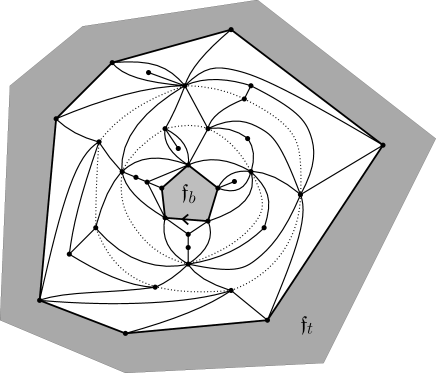
Figure 3: A truncated quadrangulation $\mathcal{Q}$ of the cylinder of height $3$ with boundary sizes $(5,7)$.The two dotted cycles represent $\partial_{1}\mathcal{Q}$ and $\partial_{2}\mathcal{Q}$ respectively (see Section 2.3 below for the definition of $\partial_{k}\mathcal{Q}$).

By definition, the inner faces of $\mathcal{Q}$ are all faces except the two distinguished ones. The last assertion of Definition 2.2 shows that the top face and the bottom face do not play a symmetric role. We will implicitly assume that truncated quadrangulations of the cylinder of height $h$ are drawn in the plane so that the top face is the unbounded face, and that they are rooted in such a way that the root edge lies on the bottom cycle and is oriented clockwise. See Fig.3 for an example.

In a way similar to the truncated quadrangulations of Definition 2.1, the triangular face associated with an edge of the bottom cycle must contain a vertex which does not belong to this cycle. The same holds for the top cycle — this is obvious from the last assertion of Definition 2.2.

2.2 Truncated quadrangulations in the UIPQ

Let us now explain why the definitions of the previous section are relevant to our study of the UIPQ. We label vertices of the UIPQ by their graph distance from the root vertex. Then the labels of corners incident to a face (enumerated in cyclic order along the boundary of the face) are of the type $k,k-1,k,k-1$ or $k,k+1,k,k-1$ for some integer $k\geq 1$, and the face is called $k$-simple in the second case. Fix an integer $r\geq 1$. For every $r$-simple face, we draw a diagonal between the two corners labeled $r$ in this face, and these diagonals are called $r$-diagonals. If $v$ is a vertex incident to an $r$-diagonal (equivalently, if $v$ has label $r$ and is incident to an $r$-simple face), then a simple combinatorial argument shows that the number of $r$-diagonals incident to $v$ is even — to be precise, we need to count this number with multiplicities, since $r$-diagonals may be loops. It follows that the collection of all $r$-diagonals can be obtained as the union of a collection of disjoint simple cycles (disjoint here means that no edge is shared by two of these cycles). See Fig.4 for an example.

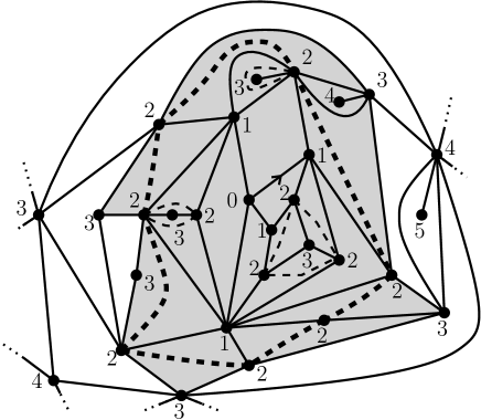
Figure 4: The UIPQ near the root vertex. Figures correspond to graph distances from the root vertex. The dashed lines show the cycles made of $r$-diagonals, for $r=2$, and the cycle in thick dashed lines is the maximal one. The shaded part is the standard hull of radius $2$. Note that the standard hull contains the truncated hull of the same radius, which is the part delimited by the maximal cycle.

Lemma 5.

There is a unique simple cycle made of $r$-diagonals such that the unbounded component of the complement of this cycle contains no $r$-diagonal and no vertex at distance less than or equal to $r$ from the root vertex. This cycle will be called the maximal cycle made of $r$-diagonals and will be denoted by $\mathcal{C}_{r}$.

Proof.

It suffices to verify that the root vertex lies inside a bounded component of the complement of some cycle made of $r$-diagonals (this cycle may be taken to be simple and then satisfies the properties stated in the lemma). To this end, consider a geodesic $\gamma$ from the root vertex to infinity and write $v_{r}$, resp. $v_{r-1},v_{r+1}$, for the unique vertex of $\gamma$ at distance $r$, resp. $r-1,r+1$, from the root vertex. Also write ${v_{r}v_{r-1}}$, resp. ${v_{r}v_{r+1}}$, for the edge of $\gamma$ incident to $v_{r}$ and $v_{r-1}$, resp. to $v_{r}$ and $v_{r+1}$. Let $k_{1}$, resp. $k_{2}$, denote the number of $r$-diagonals incident to $v_{r}$ that lie between ${v_{r}v_{r+1}}$ and ${v_{r}v_{r-1}}$, resp. between ${v_{r}v_{r-1}}$ and ${v_{r}v_{r+1}}$, when turning around $v_{r}$ in clockwise order (self-loops are counted twice). An easy combinatorial argument shows that both $k_{1}$ and $k_{2}$ are odd. It follows that there must exist a cycle made of $r$-diagonals that starts with an edge lying between ${v_{r}v_{r+1}}$ and ${v_{r}v_{r-1}}$ (in clockwise order) and ends with an edge lying between ${v_{r}v_{r-1}}$ and ${v_{r}v_{r+1}}$. Simple topological considerations now show that the root vertex, and in fact the whole geodesic path $\gamma$ up to vertex $v_{r-1}$ must lie in a bounded component of the complement of this cycle. ∎

If we now add all edges of $\mathcal{C}_{r}$ to the UIPQ and then remove all edges that lie in the unbounded component of the complement of $\mathcal{C}_{r}$, we get a truncated quadrangulation in the sense of Definition 2.1 (with the minor difference that, assuming that we keep the same root as in the UIPQ, the root edge does not belong to the boundary of the distinguished face). This truncated quadrangulation is called the truncated hull of radius $r$ and is denoted by $\mathcal{H}^{\mathrm{tr}}_{r}$. Its boundary size (the length of $\mathcal{C}_{r}$) is called the perimeter of the hull and denoted by $H_{r}$. Notice that, by construction, any vertex belonging to the boundary of the distinguished face is at distance exactly $r$ from the root vertex. Furthermore, for any vertex $v$ of the UIPQ that does not belong to $\mathcal{H}^{\mathrm{tr}}_{r}$ (equivalently, that lies in the unbounded component of the complement of $\mathcal{C}_{r}$) there exists a path going from $v$ to infinity that visits only vertices with label at least $r$. This property follows from the fact that any two points of $\mathcal{C}_{r}$ are connected by a path that visits only vertices with label at least $r$.

We may and will sometimes view the truncated hull $\mathcal{H}^{\mathrm{tr}}_{r}$ as a quadrangulation of the cylinder: To this end, we just split the root edge into a double edge, and insert a loop (based on the root vertex) inside the resulting $2$-gon. This yields a truncated quadrangulation of the cylinder of height $r$ with boundary sizes $(1,H_{r})$, whose top cycle is $\mathcal{C}_{r}$. The root edge is the inserted loop as required in our conventions. See Fig.5 for an illustration.

Figure 5: Viewing the hull $\mathcal{H}^{\mathrm{tr}}_{r}$ as a quadrangulation of the cylinder: The root edge is split in a double edge, and a loop is inserted inside the resulting $2$-gon.

Similarly, if $1\leq r<r^{\prime}$, we can consider the part of the UIPQ that lies between the cycles $\mathcal{C}_{r}$ and $\mathcal{C}_{r^{\prime}}$. More precisely, we add all edges of $\mathcal{C}_{r}$ and $\mathcal{C}_{r^{\prime}}$ to the UIPQ and then remove all edges that lie either inside the cycle $\mathcal{C}_{r}$ or outside the cycle $\mathcal{C}_{r^{\prime}}$. This gives rise to a quadrangulation of the cylinder of height $r^{\prime}-r$ whose bottom cycle and top cycle are $\mathcal{C}_{r}$ and $\mathcal{C}_{r^{\prime}}$ respectively (we in fact need to specify the root edge on the bottom cycle, but we will come back to this later). By definition, this is the annulus $\mathcal{C}(r,r^{\prime})$. We can extend this definition to $r=0$: The annulus $\mathcal{C}(0,r^{\prime})$ is just the truncated hull $\mathcal{H}^{\mathrm{tr}}_{r^{\prime}}$ viewed as a quadrangulation of the cylinder (we can also say that it is the part of the UIPQ that lies between the cycles $\mathcal{C}_{0}$ and $\mathcal{C}_{r^{\prime}}$, if $\mathcal{C}_{0}$ consists of the loop added as explained above).

As an important remark, we note that the truncated hull of radius $r$ is quite different from the (usual) hull of radius $r$ considered e.g. in [6, 7], which is denoted by $B^{\bullet}_{r}({\mathcal{P}})$ and is obtained by filling in the bounded holes in the ball of radius $r$ (recall that the ball of radius $r\geq 1$ is obtained as the union of all faces incident to at least one vertex whose graph distance from the root vertex is at most $r-1$). To avoid any ambiguity, the hull $B^{\bullet}_{r}({\mathcal{P}})$ will be called the standard hull of radius $r$. The truncated hull can be recovered from the standard hull by considering the maximal cycle made of $r$-diagonals as explained above. On the other hand, the standard hull is “bigger” than the truncated hull: To recover the standard hull from the truncated hull, we need to add the triangles incident to $r$-diagonals that have been cut when removing the unbounded component of the complement of the maximal cycle, but also to fill in the bounded holes that may appear when adding these triangles (see Fig.4 for an example). For future use, we notice that the boundary of the standard hull $B^{\bullet}_{r}({\mathcal{P}})$ is a simple cycle, and that the graph distances of vertices in this cycle to the root vertex alternate between the values $r$ and $r+1$: Those vertices at graph distance $r$ also belong to the cycle $\mathcal{C}_{r}$, but in general there are other vertices of $\mathcal{C}_{r}$ that do not belong to the boundary of $B^{\bullet}_{r}({\mathcal{P}})$ (see Fig.4).

2.3 The skeleton decomposition

We will now describe a decomposition of quadrangulations of the cylinder in layers. This is essentially due to Krikun [14] and very similar to the case of triangulations, which is treated in [13, 8]. For this reason, we will skip some details.

Let us fix a quadrangulation $\mathcal{Q}$ of the cylinder of height $h\geq 2$ with boundary sizes $(p,q)$. Assign to each vertex a label equal to its distance from the bottom boundary. Let $k\in\{1,2,\ldots,h-1\}$, and consider all diagonals connecting corners labeled $k$ in $k$-simple faces (defined in exactly the same manner as in the previous section for the UIPQ). As in the case of the UIPQ described above, these diagonals form a collection of cycles, and there is a maximal cycle which is simple and has the property that the unbounded component of the complement of this cycle contains no vertex with label less than or equal to $k$. Define the hull $\mathcal{H}_{k}(\mathcal{Q})$ by first adding to $\mathcal{Q}$ the edges of this maximal cycle and then removing all edges that lie in the unbounded component of the complement of the maximal cycle. We obtain a quadrangulation of the cylinder of height $k$ with boundary sizes $(p,q_{k})$, where $q_{k}$ denotes the size of the maximal cycle. We write $\mathcal{H}^{\mathrm{tr}}_{k}(\mathcal{Q})$ for this quadrangulation of the cylinder, and $\partial_{k}\mathcal{Q}$ for its top cycle , so that $q_{k}=|\partial_{k}\mathcal{Q}|$. See Fig.3 for the cycles $\partial_{k}\mathcal{Q}$ in a particular example.

Suppose now that we add to $\mathcal{Q}$ all diagonals drawn in the previous procedure, for every $1\leq k\leq h-1$ (in other words, we add the cycles $\partial_{k}\mathcal{Q}$ for every $1\leq k\leq h-1$), and write $\mathcal{Q}^{\bullet}$ for the resulting planar map (whose faces, except for the two distinguished faces of $\mathcal{Q}$, are either quadrangles or triangles). For every $1\leq k\leq h$, the $k$-th layer of $\mathcal{Q}$ is obtained as the part of $\mathcal{Q}^{\bullet}$ that lies between the cycles $\partial_{k-1}\mathcal{Q}$ and $\partial_{k}\mathcal{Q}$, where by convention $\partial_{0}\mathcal{Q}$ is the bottom cycle of $\mathcal{Q}$ and $\partial_{h}\mathcal{Q}$ is the top cycle. We can view this layer as a quadrangulation of the cylinder of height $1$ with boundary sizes $(|\partial_{k-1}\mathcal{Q}|,|\partial_{k}\mathcal{Q}|)$ (except that we have not specified the choice of the root edge — we will come back to this later in the case of interest to us).

We will now introduce an unordered forest $\mathcal{F}(\mathcal{Q})$ of (rooted) plane trees that in some sense describes the configuration of layers. First note that, for every $1\leq k\leq h$, each edge of $\partial_{k}\mathcal{Q}$ is incident to a unique triangle of $\mathcal{Q}^{\bullet}$ whose third vertex lies on $\partial_{k-1}\mathcal{Q}$ (when $k=h$, this is a consequence of the last assertion of Definition 2.2, and when $k<h$ this follows from the way we constructed the triangles incident to the top boundary of $\mathcal{H}^{\mathrm{tr}}_{k}(\mathcal{Q})$). We call such triangles downward triangles of $\mathcal{Q}^{\bullet}$ (see the left side of Fig.6). The forest $\mathcal{F}(\mathcal{Q})$ consists of exactly $q$ trees, each tree being associated with an edge of $\partial_{h}\mathcal{Q}$. The vertex set of the forest is the collection of all edges of $\partial_{k}\mathcal{Q}$, for $0\leq k\leq h$. The genealogical relation is specified as follows: The roots of the trees are the edges of $\partial_{h}\mathcal{Q}$, and, for every $k\in\{0,\ldots,h-1\}$, an edge $e$ of $\partial_{k}\mathcal{Q}$ is a “child” of an edge $e^{\prime}$ of $\partial_{k+1}\mathcal{Q}$ if and only if the downward triangle associated with $e^{\prime}$ (i.e., containing $e^{\prime}$ in its boundary) is the first one that one encounters when turning around $\partial_{k-1}\mathcal{Q}$ in clockwise order, starting from the middle of the edge $e$. This definition should be clear from the right side of Fig.6. Notice that edges of $\partial_{k}\mathcal{Q}$ correspond to vertices of the forest $\mathcal{F}(\mathcal{Q})$ at generation $h-k$, for every $0\leq k\leq h$. The planar structure of each tree in the forest is obviously induced by the planar structure of $\mathcal{Q}$, see again Fig.6.

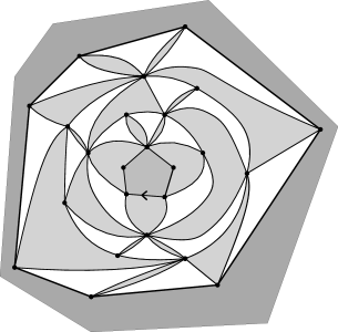
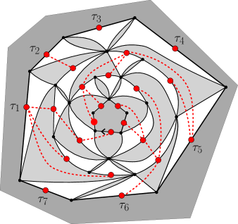
Figure 6: On the left side, the downward triangles, in white, and the slots, in light grey, in the truncated quadrangulation of Fig.3. Notice that each edge incident to two downward triangles has been split in a double edge, to emphasize the fact that this creates a slot which is a two-gon (whose filling leads to gluing the two sides of the two-gon in Fig.3). On the right side, the red dashed lines are the edges of the trees $\tau_{1},\ldots,\tau_{7}$ of the forest coding the configuration of downward triangles (notice that $\tau_{3},\tau_{4},\tau_{7}$ are trivial trees consisting only of their root vertex). The roots of the trees in the forest are the edges of the top cycle, and the trees grow “toward” the bottom cycle.

We note that the root edge of $\mathcal{Q}$ is a vertex of $\mathcal{F}(\mathcal{Q})$ at generation $h$ and belongs to one of the trees of $\mathcal{F}(\mathcal{Q})$, which we denote by $\tau_{1}$. We may then write $\tau_{2},\ldots,\tau_{q}$ for the other trees of of $\mathcal{F}(\mathcal{Q})$ listed in clockwise order from $\tau_{1}$. Without risk of confusion, we keep the notation $\mathcal{F}(\mathcal{Q})$ for the ordered forest $(\tau_{1},\ldots,\tau_{q})$.

The ordered forest $\mathcal{F}(\mathcal{Q})$ characterizes the combinatorial structure of the downward triangles in $\mathcal{Q}$. To determine $\mathcal{Q}$ completely, one also needs to specify the way “slots” between two successive downward triangles in a given layer are filled in. More precisely, let $e$ be an edge of $\partial_{k}\mathcal{Q}$, for some $1\leq k\leq h$, and let $\tilde{e}$ be the edge of $\partial_{k}\mathcal{Q}$ preceding $e$ in clockwise order (we discuss below the case when there is only one edge in $\partial_{k}\mathcal{Q}$). The part of the $k$-th layer of $\mathcal{Q}$ between the downward triangle associated with $\tilde{e}$ and the downward triangle associated with $e$ produces a slot with perimeter $c_{e}+2$, where $c_{e}$ is the number of children of $e$ in the forest $\mathcal{F}(\mathcal{Q})$. This slot is said to be associated with $e$ (it is also incident to a unique vertex $v$ of $\partial_{k}\mathcal{Q}$). See the left side of Fig.7 for an illustration. If $c_{e}=0$, it may happen that the slot is empty, if the downward triangles associated with $\tilde{e}$ and $e$ are adjacent. Also notice that when $|\partial_{k}\mathcal{Q}|=1$, the only edge of $\partial_{k}\mathcal{Q}$ is a loop, but there is still an associated slot, which is bounded by the double edge in the boundary of the downward triangle associated with the unique edge of $\partial_{k}\mathcal{Q}$, and the edges of $\partial_{k-1}\mathcal{Q}$.

The boundary of the slot associated with $e$ is of the type pictured in the left side of Fig.7, where there are $c_{e}$ horizontal edges and the two non-horizontal edges are incident to the downward triangles associated with $\tilde{e}$ and $e$. Strictly speaking, the random planar map consisting of the part of $\mathcal{Q}^{\bullet}$ in the slot is not a truncated quadrangulation with a boundary, but a simple transformation allows us to view it as a truncated quadrangulation with a boundary of size $c_{\tilde{e}}+1$: this transformation, which involves adding an extra edge, is illustrated in Fig.7 (see also Fig.6 in [14]) — to be precise, one should notice that the two vertices $a$ and $b$ in Fig.7 may be the same if all edges of $\partial_{k-1}\mathcal{Q}$ have the same “parent” in $\partial_{k}\mathcal{Q}$, but our interpretation still goes through. There is therefore a one-to-one correspondence between possible fillings of the slot and such truncated quadrangulations. To make this correspondence precise, we need a convention for the position of the root: we can declare that in the filling of the slot, the root edge of the truncated quadrangulation corresponds to the added extra edge. We notice that, in the special case where $c_{e}=0$, if the truncated quadrangulation used to fill in the slot is the unique truncated quadrangulation with boundary size $1$ and no quadrangle, this means that the slot is empty so that two sides of the downward triangles associated with $\tilde{e}$ and $e$ are glued together.

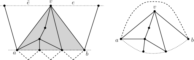
Figure 7: On the left side, the shaded part corresponds to the slot associated with an edge $e$ of $\partial_{k}\mathcal{Q}$, such that $c_{e}=3$. This slot is bounded by the two “vertical edges” $av$ and $bv$ (which are incident to the downward triangles associated with $\tilde{e}$ and $e$ respectively) and by three diagonals (in dotted lines between $a$ and $b$). On the right side, this slot is viewed as a truncated triangulation with boundary size $4$ by adding the edge between $a$ and $b$ in dashed lines.

Following [8], we say that a forest $\mathcal{F}$ with a distinguished vertex is $(h,p,q)$-admissible if

1. the forest consists of an ordered sequence $({\mathcal{T}}_{1},{\mathcal{T}}_{2},\ldots,{\mathcal{T}}_{q})$ of $q$ (rooted) plane trees,

2. the maximal height of these trees is $h$,

3. the total number of vertices of the forest at generation $h$ is $p$,

4. the distinguished vertex has height $h$ and belongs to ${\mathcal{T}}_{1}$.

If $\mathcal{F}$ is a $(h,p,q)$-admissible forest, we write $\mathcal{F}^{*}$ for the set all vertices of $\mathcal{F}$ at height strictly less than $h$. We write ${\mathbb{F}}^{\circ}_{h,p,q}$ for the set of all $(h,p,q)$-admissible forests.

The preceding discussion yields a bijection between, on the one hand, truncated quadrangulations $\mathcal{Q}$ of the cylinder of height $h$ with boundary sizes $(p,q)$, and, on the other hand, pairs consisting of a $(h,p,q)$-admissible forest $\mathcal{F}$ and a collection $(M_{v})_{v\in\mathcal{F}^{*}}$ such that, for every $v\in\mathcal{F}^{*}$, $M_{v}$ is a truncated quadrangulation with boundary size $c_{v}+1$, if $c_{v}$ stands for the number of children of $v$ in $\mathcal{F}$. We call this bijection the skeleton decomposition and we say that $\mathcal{F}$ is the skeleton of the quadrangulation $\mathcal{Q}$.

It will also be convenient to use the notation ${\mathbb{F}}_{h,p,q}$ for the set of all (ordered) forests, with no distinguished vertex, that satisfy properties (i),(ii),(iii) above. If $\mathcal{F}\in{\mathbb{F}}_{h,p,q}$, we keep the notation $\mathcal{F}^{*}$ for the set all vertices of $\mathcal{F}$ at height strictly less than $h$.

We also set, for every $p\geq 1$, $h\geq 1$,

$${\mathbb{F}}^{\circ}_{h,p}=\bigcup_{q\geq 1}{\mathbb{F}}^{\circ}_{h,p,q}\;,\qquad{\mathbb{F}}_{h,p}=\bigcup_{q\geq 1}{\mathbb{F}}_{h,p,q}.$$

We conclude this section with a useful observation about connections between the truncated hull and the standard hull of the UIPQ. Consider two integers $u$ and $r$ with $1\leq u<r$. Recall that the truncated hull $\mathcal{H}^{\mathrm{tr}}_{r}$ is viewed as a truncated quadrangulation of the cylinder of height $r$, whose top cycle is $\mathcal{C}_{r}$. Write $\mathcal{F}^{\circ}_{(r)}$ for the skeleton of this truncated quadrangulation, and also consider the cycle $\partial_{u}\mathcal{H}^{\mathrm{tr}}_{r}$, which by construction coincides with $\mathcal{C}_{u}$. Vertices of this cycle are at distance $u$ from the root vertex of the UIPQ, and may or may not belong to the boundary of the standard hull of radius $u$. However, assuming that $|\mathcal{C}_{u}|>1$, if a vertex $v$ of the cycle $\mathcal{C}_{u}$ is such that the parents (in the forest $\mathcal{F}^{\circ}_{(r)}$) of the two edges of $\mathcal{C}_{u}=\partial_{u}\mathcal{H}^{\mathrm{tr}}_{r}$ incident to $v$ are different edges of the cycle $\mathcal{C}_{u+1}=\partial_{u+1}\mathcal{H}^{\mathrm{tr}}_{r}$, then $v$ must belong to the boundary of the standard hull of radius $u$. We leave the easy verification of this combinatorial fact to the reader. Notice that this is only a sufficient condition and that vertices of $\mathcal{C}_{u}$ that do not satisfy this condition may also belong to the boundary of the standard hull of radius $u$.

2.4 Geodesics in the skeleton decomposition

Consider again a quadrangulation $\mathcal{Q}$ of the cylinder of height $h\geq 2$ with boundary sizes $(p,q)$. Let $v$ be a vertex of $\partial_{k}\mathcal{Q}$ for some $k\in\{1,\ldots,h\}$. We assume that $|\partial_{k}\mathcal{Q}|\geq 2$. Then $v$ is incident to two downward triangles which both contain an edge of $\partial_{k}\mathcal{Q}$ and a vertex of $\partial_{k-1}\mathcal{Q}$. Each of these triangles has an edge incident both to $v$ and to a vertex of $\partial_{k-1}\mathcal{Q}$, and these two edges (which may be the same if the slot incident to $v$ in the $k$-th layer of $\mathcal{Q}$ is empty) are called downward edges from $v$. If the slot incident to $v$ is nonempty we can in fact define the left downward edge by declaring that it is the first (downward) edge visited when exploring the boundary of the slot in clockwise order starting from a point of $\partial_{k-1}\mathcal{Q}$, and the other downward edge is called the right downward edge (of course if the slot is empty, the left and right downward edges coincide). We leave it to the reader to adapt these definitions in the case $|\partial_{k}\mathcal{Q}|=1$ — in that case the left and right downward edges form a double edge.

We then define the left downward geodesic from $v$ by saying that we first follow the left downward edge from $v$ to arrive at a vertex $v^{\prime}$ of $\partial_{k-1}\mathcal{Q}$, then the left downward edge from $v^{\prime}$ to a vertex $v^{\prime\prime}$ of $\partial_{k-2}\mathcal{Q}$, and so on until we reach the bottom cycle $\partial_{0}\mathcal{Q}$. Similarly we define the right downward geodesic from $v$ by choosing at the first step the right downward edge from $v$, but then, as previously, following left downward edges from the visited vertices. See Fig.8 for an illustration.

Let $N$ be the number of trees with maximal height in the skeleton decomposition of $\mathcal{Q}$. Assume that $N\geq 2$, which implies that $|\partial_{k}\mathcal{Q}|\geq 2$ for every $k\in\{0,1,\ldots,h\}$. Let $e$ be an edge of $\partial_{h}\mathcal{Q}$ corresponding to a tree with maximal height, and let $v$ be the first vertex incident to $e$ in clockwise order around $\partial_{h}\mathcal{Q}$. Then the left downward geodesic (resp. the right downward geodesic) from $v$ hits the bottom cycle at a vertex $v_{1}$ (resp. at $v_{2}$) such that the edges of the bottom cycle lying between $v_{1}$ and $v_{2}$ in clockwise order are exactly the descendants of $e$ at generation $h$ in the skeleton decomposition. See Fig.8 for an example. The concatenation of these two geodesic paths gives a path from $v_{1}$ to $v_{2}$ with length $2h$. If we vary the edge $e$ among all roots of trees with maximal height, we can concatenate the resulting paths to get a cycle $\mathcal{C}$ with length $2Nh$, such that any path from the bottom cycle to the top cycle must visit a vertex of $\mathcal{C}$. In particular, if $\mathcal{Q}$ is the annulus $\mathcal{C}(R,R+h)$ in the UIPQ, with $R\geq 3$, the cycle $\mathcal{C}$ disconnects the ball $B_{R-2}({\mathcal{P}})$ (or the hull $B^{\bullet}_{R-2}({\mathcal{P}})$) from infinity.

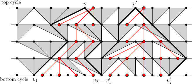
Figure 8: A portion of a truncated quadrangulation of the cylinder of height $4$. The downward triangles are colored in grey, and the associated slots are in white (they should of course be “filled in” by truncated quadrangulations as explained in the text). Two successive trees with maximal height in the coding forest are represented in red. The thick black lines are the (left and right) downward geodesics from the vertices $v$ and $v^{\prime}$ of the top cycle associated with the two trees.

2.5 Enumeration

We rely on the results of Krikun [14]. Recall that ${\mathbb{Q}}^{\mathrm{tr}}_{n,p}$ is the set of all truncated quadrangulations with boundary size $p$ and $n$ inner faces (this set is empty if $n<p$).

Section 2.2 of Krikun [14] provides an explicit formula for the generating function

$$U(x,y)=\sum_{p=1}^{\infty}\sum_{n=1}^{\infty}\#{\mathbb{Q}}^{\mathrm{tr}}_{n,p}\ x^{n}y^{p}.$$

We will not need this formula, but we record the special case

$$U(\frac{1}{12},y)=\frac{1}{24}\sqrt{(18-y)(2-y)^{3}}-\frac{1}{2}+\frac{y}{2}-\frac{y^{2}}{24},$$ (1)

for $0\leq y<2$.

As a consequence of the explicit formula for the generating function $U$, we have, for every fixed $p\geq 1$,

$$\#{\mathbb{Q}}^{\mathrm{tr}}_{n,p}\mathrel{\mathop{\kern 0.0pt\sim}\limits_{n\to\infty}}\kappa_{p}\,n^{-5/2}\,12^{n},$$ (2)

where the constants $\kappa_{p}$ are determined by the generating function

$$\sum_{p=1}^{\infty}\kappa_{p}\,y^{p}=\frac{128\sqrt{3}}{\sqrt{\pi}}\,\frac{y}{\sqrt{(18-y)(2-y)^{3}}}.$$ (3)

for $0\leq y<2$. We again refer to [14, Section 2.2] for these results. From (3) and standard singularity analysis [11, Corollary VI.1], we get

$$\kappa_{p}\mathrel{\mathop{\kern 0.0pt\sim}\limits_{p\to\infty}}\frac{64\sqrt{3}}{\pi\sqrt{2}}\,\sqrt{p}\,2^{-p}.$$ (4)

We also note that

$$\kappa_{1}=\frac{32}{\sqrt{3\pi}}.$$

2.6 The distribution of hulls

Fix integers $n$ and $p$ with $n\geq p$. Let $\mathcal{Q}^{(n)}_{p}$ be uniformly distributed over ${\mathbb{Q}}^{\mathrm{tr}}_{n,p}$ and given with a distinguished vertex chosen uniformly at random. Let $r\geq 1$. If the height (distance from the boundary) of this distinguished vertex is at least $r+1$, we can make sense of the hull $\mathcal{H}_{r}(\mathcal{Q}^{(n)}_{p})$. To this end, we label each vertex by its graph distance from the boundary of the distinguished face, and we proceed in a way very similar to the case of the UIPQ discussed in Section 2.2. We consider all diagonals connecting corners labeled $r$ in $r$-simple faces (of type $r-1,r,r+1,r$), and the maximal cycle made of these diagonals, which has the property that the connected component of the complement of this cycle containing the distinguished vertex contains only vertices whose label is greater than $r$. We then add to $\mathcal{Q}^{(n)}_{p}$ the edges of this maximal cycle, and remove all edges lying in the connected component of the complement of this cycle containing the distinguished vertex. In this way, we obtain the hull $\mathcal{H}_{r}(\mathcal{Q}^{(n)}_{p})$, and it is easy to verify that $\mathcal{H}_{r}(\mathcal{Q}^{(n)}_{p})$ is a quadrangulation of the cylinder of height $r$ (the size of its bottom cycle is $p$). If the height of the distinguished vertex is smaller than or equal to $r$, the preceding definition no longer makes sense, but by convention we define $\mathcal{H}_{r}(\mathcal{Q}^{(n)}_{p})=\dagger$ to be some “cemetery point” added to the set of all quadrangulations of the cylinder of height $r$.

The next lemma, which is an analog of Lemma 2 in [8], shows that the distribution of $\mathcal{H}_{r}(\mathcal{Q}^{(n)}_{p})$ has a limit when $n\to\infty$. We let $\mathcal{Q}$ be a fixed quadrangulation of the cylinder of height $r$ with boundary sizes $(p,q)$. This quadrangulation is coded by an $(r,p,q)$-admissible forest $\mathcal{F}$ and a collection $(M_{v})_{c\in\mathcal{F}^{*}}$, such that, for every $v\in\mathcal{F}^{*}$, $M_{v}$ is a truncated quadrangulation with boundary size $c_{v}+1$. Let $\mathsf{Inn}(M_{v})$ denote the number of inner faces of $M_{v}$.

Lemma 6.

We have

$$\lim_{n\to\infty}{\mathbb{P}}(\mathcal{H}_{r}(\mathcal{Q}^{(n)}_{p})=\mathcal{Q})=\frac{2^{q}\kappa_{q}}{2^{p}\kappa_{p}}\,\prod_{v\in\mathcal{F}^{*}}\Bigg{(}\theta(c_{v})\,\frac{12^{-\mathsf{Inn}(M_{v})}}{Z(c_{v}+1)}\Bigg{)}$$ (5)

where, for every $k\geq 1$,

$$Z(k)=\sum_{n=k}^{\infty}\#{\mathbb{Q}}^{\mathrm{tr}}_{n,k}\,12^{-n},$$

and $\theta$ is the critical offspring distribution defined by

$$\theta(k)=6\cdot 2^{k}\,Z(k+1).$$

The generating function of $\theta$ is given for $0\leq y<1$ by

$$g_{\theta}(y)=1-\frac{8}{\Big{(}\sqrt{\frac{9-y}{1-y}}+2\Big{)}^{2}-1}.$$ (6)

We note that the property $Z(k)<\infty$ follows from (2).

Proof.

We proceed in a very similar way to the proof of Lemma 2 in [8]. Let $N$ be the number of inner faces of $\mathcal{Q}$, which is also the total number of vertices of $\mathcal{Q}$ (by Euler’s formula). We observe that the property $\mathcal{H}_{r}(\mathcal{Q}^{(n)}_{p})=\mathcal{Q}$ holds if and only if $\mathcal{Q}^{(n)}_{p}$ is obtained from $\mathcal{Q}$ by gluing on the top boundary of $\mathcal{Q}$ an arbitrary truncated quadrangulation with boundary size $q$ and $n-(N-q)$ inner faces (for this gluing to make sense we need to specify an edge of the top boundary of $\mathcal{Q}$, which can be the root of the first tree in the forest $\mathcal{F}$), and if the distinguished vertex of $\mathcal{Q}^{(n)}_{p}$ is chosen among the inner vertices of this truncated quadrangulation. Noting that $\mathcal{Q}^{(n)}_{p}$ has $n+1$ vertices, it follows that

$${\mathbb{P}}(\mathcal{H}_{r}(\mathcal{Q}^{(n)}_{p})=\mathcal{Q})=\frac{\#{\mathbb{Q}}^{\mathrm{tr}}_{n-(N-q),q}}{\#{\mathbb{Q}}^{\mathrm{tr}}_{n,p}}\times\frac{n+1-N}{n+1}.$$

Using (2), we get

$$\lim_{n\to\infty}{\mathbb{P}}(\mathcal{H}_{r}(\mathcal{Q}^{(n)}_{p})=\mathcal{Q})=\frac{\kappa_{q}}{\kappa_{p}}\,12^{-N+q}.$$ (7)

Simple combinatorics shows that the number of inner faces of $\mathcal{Q}$ can be written as

$$N=p+\sum_{v\in\mathcal{F}^{*}}(\mathsf{Inn}(M_{v})-c_{v}).$$ (8)

So the right-hand side of (7) is also equal to

$$\frac{\kappa_{q}}{\kappa_{p}}\,12^{q-p}\prod_{v\in\mathcal{F}^{*}}(12^{c_{v}}\,12^{-\mathsf{Inn}(M_{v})}).$$

It is now straightforward to verify that the last quantity is equal to the right-hand side of (5). Just observe that

$$12^{c_{v}}\,Z(c_{v}+1)=6^{c_{v}-1}\,\theta(c_{v})$$

and notice that

$$\sum_{v\in\mathcal{F}^{*}}(c_{v}-1)=p-q.$$

To see that $\theta$ is an offspring distribution, we rely on (1), which shows that the generating function of $\theta$ is

$$g_{\theta}(y):=\sum_{k=0}^{\infty}\theta(k)\,y^{k} =6\sum_{k=0}^{\infty}\sum_{n=k+1}^{\infty}y^{k}2^{k}12^{-n}\#{\mathbb{Q}}^{\mathrm{tr}}_{n,k+1}$$

$$=\frac{6}{2y}\,U(\frac{1}{12},2y)$$

$$=\frac{1}{2y}\Big{(}\sqrt{(9-y)(1-y)^{3}}-3+6y-y^{2}\Big{)},$$

in agreement with Theorem 2 of [14]. Since $g_{\theta}(1)=1$, $\theta$ is a probability distribution, and the fact that $\theta$ is critical is obtained by checking that $g_{\theta}^{\prime}(1)=1$.

Finally, a somewhat tedious calculation shows that the formula for $g_{\theta}$ in the last display is equivalent to the one given in the statement of the lemma. The latter is more convenient to compute iterates of $g_{\theta}$, as we will see below in formula (15). ∎

From the explicit form of $g_{\theta}$, we have

$$g_{\theta}(1-x)=1-x+\sqrt{2}\,x^{3/2}+O(x^{2})$$

as $x\downarrow 0$. By singularity analysis, it follows that

$$\theta(k)\mathrel{\mathop{\kern 0.0pt\sim}\limits_{k\to\infty}}\frac{3\sqrt{2}}{4\sqrt{\pi}}\,k^{-5/2}.$$ (9)

Remark. The offspring distribution $\theta$ appears in the seemingly different context of labeled trees. Consider a critical Galton-Watson tree with geometric offspring distribution with parameter $1/2$. Given the tree, assign labels to vertices by declaring that the label of the root is $0$ and that label increments on different edges are independent and uniformly distributed over $\{-1,0,1\}$. Let $N$ be the number of vertices labeled $-1$ whose (strict) ancestors all have nonnegative labels. Then $N$ is distributed according to $\theta$ (see [9, Proof of Theorem 5.2]). Via Schaeffer’s bijection relating plane quadrangulations to labeled trees, this interpretation of $\theta$ is in fact closely related to Lemma 6.

We define, for every $p\geq 1$,

$$h(p):=\frac{1}{p}\,2^{p}\,\kappa_{p}.$$ (10)

Lemma 7.

Let $p\geq 1$. The formula

$$\mu_{r,p}(\mathcal{F}):=\frac{h(q)}{h(p)}\,\prod_{v\in\mathcal{F}^{*}}\theta(c_{v})\;,\ \mathcal{F}\in{\mathbb{F}}_{r,p,q},\,q\geq 1$$

defines a probability measure on ${\mathbb{F}}_{r,p}$. Consequently, the formula

$$\mu^{\circ}_{r,p}(\mathcal{F}):=\frac{2^{q}\kappa_{q}}{2^{p}\kappa_{p}}\,\prod_{v\in\mathcal{F}^{*}}\theta(c_{v})\;,\ \mathcal{F}\in{\mathbb{F}}^{\circ}_{r,p,q},\,q\geq 1$$

defines a probability measure on ${\mathbb{F}}^{\circ}_{r,p}$.

Proof.

Let $\Pi$ be the generating function of the sequence $(h(k))_{k\geq 1}$,

$$\Pi(x):=\sum_{k=1}^{\infty}h(k)\,x^{k}.$$

To verify that $\mu_{r,p}$ defines a probability distribution on the set ${\mathbb{F}}_{r,p}$, it is enough to check that $(h(k))_{k\geq 1}$ is an (infinite) stationary measure for the branching process with offspring distribution $\theta$, or equivalently that, for every $0<y<1$,

$$\Pi(g_{\theta}(y))-\Pi(g_{\theta}(0))=\Pi(y).$$ (11)

From (3), we get by integration that

$$\sum_{p=1}^{\infty}\kappa_{p}\,\frac{x^{p}}{p}=\frac{48}{\sqrt{\pi}}\,\Bigg{(}\sqrt{\frac{18-x}{3(2-x)}}-\sqrt{3}\Bigg{)},$$

and, for $0<x<1$,

$$\Pi(x)=\frac{48}{\sqrt{3\pi}}\,\Bigg{(}\sqrt{\frac{9-x}{1-x}}-3\Bigg{)}.$$

From this explicit formula and (6), the desired identity (11) follows at once.

Once we know that $\mu_{r,p}$ is a probability distribution on ${\mathbb{F}}_{r,p}$, the fact that $\mu^{\circ}_{r,p}$ is a probability distribution on ${\mathbb{F}}^{\circ}_{r,p}$ follows easily. First note that

$$\tilde{\mu}((\mathcal{F},v)):=\frac{1}{p}\,\mu_{r,p}(\mathcal{F})$$

defines a probability distribution on the set of all pairs $(\mathcal{F},v)$ consisting of a forest $\mathcal{F}\in{\mathbb{F}}_{r,p}$ and a distinguished vertex $v$ of $\mathcal{F}$ at generation $r$. Then notice that $\mu^{\circ}_{r,p}$ is just the push forward of $\tilde{\mu}$ under the mapping $(\mathcal{F},v)\mapsto\mathcal{F}^{\prime}$, where $\mathcal{F}^{\prime}$ is obtained by circularly permuting the trees of $\mathcal{F}$ so that $v$ belongs to the first tree of the forest. This completes the proof. ∎

Let us consider now the UIPQ. Recall our notation $\mathcal{H}^{\mathrm{tr}}_{r}$ for the truncated hull of radius $r$, and $H_{r}$ for the perimeter of $\mathcal{H}^{\mathrm{tr}}_{r}$, which is also the length of the cycle $\mathcal{C}_{r}$. For every $r,p\geq 1$, let ${\mathbb{C}}_{r,p}$ be the set of all truncated quadrangulations of the cylinder of height $r$ with bottom boundary size $p$ and arbitrary top boundary size. If $\mathcal{Q}\in{\mathbb{C}}_{r,p}$ and the size of the top boundary of $\mathcal{Q}$ is $q$, we set

$$\Delta_{r,p}(\mathcal{Q})=\frac{2^{q}\kappa_{q}}{2^{p}\kappa_{p}}\,\prod_{v\in\mathcal{F}^{*}}\Bigg{(}\theta(c_{v})\,\frac{12^{-\mathsf{Inn}(M_{v})}}{Z(c_{v}+1)}\Bigg{)},$$

where $(\mathcal{F},(M_{v})_{v\in\mathcal{F}^{*}})$ is the skeleton decomposition of $\mathcal{Q}$.

Corollary 8.

$\Delta_{r,p}$ is a probability measure on ${\mathbb{C}}_{r,p}$. Furthermore, the distribution of $\mathcal{H}^{\mathrm{tr}}_{r}$ is $\Delta_{r,1}$.

Proof.

The fact that $\Delta_{r,p}$ is a probability measure on ${\mathbb{C}}_{r,p}$ readily follows from the second assertion of Lemma 7, noting that, by the very definition of $Z(k)$, we have

$$\sum_{n=1}^{\infty}\#{\mathbb{Q}}^{\mathrm{tr}}_{n,k+1}\,\frac{12^{-n}}{Z(k+1)}=1.$$

To get the second assertion of the corollary, let ${\mathbb{Q}}_{n}$ stand for the set of all (rooted) planar quadrangulations with $n$ faces. Via the transformation that consists in splitting the root edge to get a double edge, and then inserting a loop inside the resulting $2$-gon (as in Fig.5), the set ${\mathbb{Q}}_{n}$ is canonically identified to ${\mathbb{Q}}^{\mathrm{tr}}_{n+1,1}$. From the local convergence of planar quadrangulations to the UIPQ [14], we deduce that the distribution of the hull of radius $r$ in a uniformly distributed quadrangulation in ${\mathbb{Q}}^{\mathrm{tr}}_{n,1}$ (equipped with a distinguished uniformly distributed vertex) converges to the distribution of the hull of radius $r$ in the UIPQ. The second assertion of the corollary now follows from Lemma 6. ∎

Corollary 9.

The distribution of $H_{r}$ is given by

$${\mathbb{P}}(H_{r}=p)=\frac{h(p)}{h(1)}\,{\mathbb{P}}_{p}(Y_{r}=1),\quad p\geq 1,$$

where $(Y_{n})_{n\geq 0}$ denotes a Galton-Watson branching process with offspring distribution $\theta$ that starts from $p$ under the probability measure ${\mathbb{P}}_{p}$.

Proof.

Let $\mathcal{F}_{(r)}^{\circ}$ be the skeleton of the hull $\mathcal{H}^{\mathrm{tr}}_{r}$ viewed as a quadrangulation of the cylinder of height $r$. As a direct consequence of the second assertion of Corollary 8, $\mathcal{F}_{(r)}^{\circ}$ is distributed as $\mu^{\circ}_{r,1}$. Define $\mathcal{F}_{(r)}$ from $\mathcal{F}^{\circ}_{(r)}$ by “forgetting” the distinguished vertex and applying a uniform random circular permutation to the trees in the sequence. Arguing as in the end of the proof of Lemma 7, it follows that $\mathcal{F}_{(r)}$ is distributed according to $\mu_{r,1}$.

Since $H_{r}$ is just the number of trees in the forest $\mathcal{F}_{(r)}$, we have

$${\mathbb{P}}(H_{r}=p)=\sum_{\mathcal{F}\in{\mathbb{F}}_{r,1,p}}{\mathbb{P}}(\mathcal{F}_{(r)}=\mathcal{F})=\frac{h(p)}{h(1)}\,\sum_{\mathcal{F}\in{\mathbb{F}}_{r,1,p}}\prod_{v\in\mathcal{F}^{*}}\theta(c_{v}),$$

and the desired result follows. ∎

Remark. One can interpret the distribution of $H_{r}$ as the limit when $T\to\infty$ of the distribution at time $T-r$ of a Galton-Watson process $X$ with offspring distribution $\theta$ started from $X_{0}=1$ and conditioned on the event $\{X_{T}=1\}$. This suggests that one may code the combinatorial structure of downward triangles in the whole UIPQ (and not only in a hull of fixed radius) by an infinite tree, which could be viewed as the genealogical tree for a Galton-Watson process with offspring distribution $\theta$, indexed by nonpositive integer times and conditioned to be equal to $1$ at time $0$. This interpretation will not be needed in the present work and we omit the details.

Let us now fix integers $0\leq u<r$. As explained earlier, the annulus $\mathcal{C}({u,r})$ is the part of the UIPQ that lies between the cycles $\mathcal{C}_{u}$ and $\mathcal{C}_{r}$ — recall our convention for $\mathcal{C}_{0}$ from Section 2.2 — and $\mathcal{C}({u,r})$ is viewed as a truncated quadrangulation of the cylinder of height $r-u$ with boundary sizes $(H_{u},H_{r})$. We now specify the root edge of $\mathcal{C}({u,r})$, by declaring that it corresponds to the root of the tree, in the skeleton decomposition of $\mathcal{H}^{\mathrm{tr}}_{u}$, that carries the root edge of the UIPQ (of course when $u=0$, the root edge is the unique edge of $\mathcal{C}_{0}$).

Let $\mathcal{F}^{\circ}_{u,r}$ be the skeleton of $\mathcal{C}(u,r)$, which is a random element of $\cup_{p\geq 1}{\mathbb{F}}^{\circ}_{r-u,p}$. It will be convenient to introduce also the forest $\mathcal{F}_{u,r}$ (in $\cup_{p\geq 1}{\mathbb{F}}_{r-u,p}$) obtained from $\mathcal{F}^{\circ}_{u,r}$ by first “forgetting” the distinguished vertex and then applying a uniform random circular permutation to the trees in the sequence.

Corollary 10.

Let $p\geq 1$. The conditional distribution of $\mathcal{F}_{u,r}$ knowing that $H_{u}=p$ is $\mu_{r-u,p}$.

Proof.

Recall the notation $\mathcal{F}^{\circ}_{(r)},\mathcal{F}_{(r)}$ introduced in the previous proof. We notice that, if $(\tau_{1},\ldots,\tau_{H_{r}})$ are the trees in the forest $\mathcal{F}^{\circ}_{(r)}$, the trees in the forest $\mathcal{F}^{\circ}_{u,r}$ are just $(\tau_{1}^{[r-u]},\ldots,\tau_{H_{r}}^{[r-u]})$, where the notation $\tau_{i}^{[r-u]}$ refers to the tree $\tau_{i}$ truncated at generation $r-u$. It follows that $\mathcal{F}_{u,r}$ can be assumed to be equal to the forest $\mathcal{F}_{(r)}$ truncated at generation $r-u$. Note that $H_{u}$ is just the number of vertices of $\mathcal{F}_{(r)}$ at generation $r-u$.

Let $q\geq 1$ and $\mathcal{G}\in{\mathbb{F}}_{r-u,p,q}$. We have

$${\mathbb{P}}(\mathcal{F}_{u,r}=\mathcal{G})=\sum_{\mathcal{F}\in{\mathbb{F}}_{r,1}:\mathcal{F}^{[r-u]}=\mathcal{G}}{\mathbb{P}}(\mathcal{F}_{(r)}=\mathcal{F}),$$

using the notation $\mathcal{F}^{[r-u]}$ for the forest $\mathcal{F}$ truncated at generation $r-u$. It follows that

$${\mathbb{P}}(\mathcal{F}_{u,r}=\mathcal{G}) =\frac{h(q)}{h(1)}\sum_{\mathcal{F}\in{\mathbb{F}}_{r,1}:\mathcal{F}^{[r-u]}=\mathcal{G}}\prod_{v\in\mathcal{F}^{*}}\theta(c_{v})$$

$$=\frac{h(q)}{h(1)}\,\prod_{v\in\mathcal{G}^{*}}\theta(c_{v})\,\sum_{\tilde{\mathcal{F}}\in{\mathbb{F}}_{u,1,p}}\prod_{v\in\tilde{\mathcal{F}}^{*}}\theta(c_{v}),$$

where we just use the fact that a forest $\mathcal{F}\in{\mathbb{F}}_{r,1}$ such that $\mathcal{F}^{[r-u]}=\mathcal{G}$ is obtained by “gluing” a forest of ${\mathbb{F}}_{u,1,p}$ to the $p$ vertices of $\mathcal{G}$ at generation $r-u$. As in Corollary 9 and its proof, we have

$$\sum_{\tilde{\mathcal{F}}\in{\mathbb{F}}_{u,1,p}}\prod_{v\in\tilde{\mathcal{F}}^{*}}\theta(c_{v})={\mathbb{P}}_{p}(Y_{u}=1)=\frac{h(1)}{h(p)}\,{\mathbb{P}}(H_{u}=p).$$

So we get

$${\mathbb{P}}(\mathcal{F}_{u,r}=\mathcal{G})=\frac{h(q)}{h(p)}\prod_{v\in\mathcal{G}^{*}}\theta(c_{v})\times{\mathbb{P}}(H_{u}=p)={\mathbb{P}}(H_{u}=p)\,\mu_{r-u}(\mathcal{G}).$$

This completes the proof. ∎

2.7 The law of the perimeter of hulls

We give a more explicit formula for the distribution of $H_{r}$.

Proposition 11.

We have, for every $r\geq 1$ and $p\geq 1$,

$${\mathbb{P}}(H_{r}=p)=K_{r}\,\kappa_{p}\,(2\pi_{r})^{p}$$ (12)

where

$$\pi_{r} =1-\frac{8}{(3+2r)^{2}-1}=\frac{r(r+3)}{(r+1)(r+2)}$$

$$K_{r} =\frac{32}{3\kappa_{1}}\,\frac{3+2r}{((3+2r)^{2}-1)^{2}}\;\frac{1}{\pi_{r}}=\frac{2}{3\kappa_{1}}\,\frac{2r+3}{r(r+1)(r+2)(r+3)}.$$

Consequently, there exist positive constants $M_{1},M_{2}$ and $\rho$ such that, for every $a>0$, for every integer $r\geq 1$,

$${\mathbb{P}}(H_{r}\geq a\,r^{2})\leq M_{1}\,e^{-\rho a}$$ (13)

and

$${\mathbb{P}}(H_{r}\leq a\,r^{2})\leq M_{2}\,a^{3/2}.$$ (14)

We notice that $K_{r}\sim(4/(3\kappa_{1}))\,r^{-3}$ as $r\to\infty$ and recall that $\kappa_{1}=\frac{32}{\sqrt{3\pi}}$.

Proof.

We rely on the formula of Corollary 9. Recalling that $(Y_{n})_{n\geq 0}$ denotes a Galton-Watson branching process with offspring distribution $\theta$ that starts from $p$ under the probability measure ${\mathbb{P}}_{p}$, and using formula (6), we obtain that the generating function of $Y_{r}$ under ${\mathbb{P}}_{1}$ is

$$g^{(r)}_{\theta}(y)=\underbrace{g_{\theta}\circ\cdots\circ g_{\theta}}_{r\;{\rm times}}(y)=1-\frac{8}{\Big{(}\sqrt{\frac{9-y}{1-y}}+2r\Big{)}^{2}-1}.$$ (15)

It follows that

$${\mathbb{P}}_{1}(Y_{r}=0)=g_{\theta}^{(r)}(0)=1-\frac{8}{(3+2r)^{2}-1}=\pi_{r},$$ (16)

and

$${\mathbb{P}}_{p}(Y_{r}=1) =\lim_{x\downarrow 0}\frac{1}{x}\Big{(}{\mathbb{E}}_{p}[x^{Y_{r}}]-{\mathbb{P}}_{p}(Y_{r}=0)\Big{)}$$

$$=\lim_{x\downarrow 0}\frac{1}{x}\Big{(}g^{(r)}_{\theta}(x)^{p}-g^{(r)}_{\theta}(0)^{p}\Big{)}$$

$$=p\,g^{(r)}_{\theta}(0)^{p-1}\times\frac{64}{3}\,\frac{3+2r}{((3+2r)^{2}-1)^{2}}$$

$$=\frac{64}{3}\,p\,\frac{3+2r}{((3+2r)^{2}-1)^{2}}\,\Bigg{(}1-\frac{8}{(3+2r)^{2}-1}\Bigg{)}^{p-1}.$$ (17)

Since

$$\frac{h(p)}{h(1)}=\frac{1}{p}\,\frac{2^{p}\kappa_{p}}{2\,\kappa_{1}},$$

Corollary 9 and (2.7) lead to formula (12). Finally, the bounds (13) and (14) are simple consequences of this explicit formula and the asymptotics (4) for the constants $\kappa_{p}$. To derive (13), we observe that we can find a constant $\eta>0$ such that ${\mathbb{P}}(H_{r}\geq a\,r^{2})$ is bounded above by a constant times

$$r^{-3}\sum_{p>ar^{2}}\sqrt{p}\times e^{-\eta p/r^{2}}\leq\hbox{Cst.}\,r^{-3}\int_{ar^{2}/2}^{\infty}\sqrt{x}e^{-\eta x/r^{2}}\mathrm{d}x=\hbox{Cst.}\times\int_{a/2}^{\infty}\sqrt{y}e^{-\eta y}\mathrm{d}y,$$

and the proof of (14) is even easier just bounding $\pi_{r}$ by $1$. ∎

2.8 A conditional limit for branching processes

We keep the notation $(Y_{n})_{n\geq 0}$ for a branching process with offspring distribution $\theta$, which starts at $p$ under the probability measure ${\mathbb{P}}_{p}$.

Lemma 12.

We have

$${\mathbb{P}}_{1}(Y_{r}\not=0)\mathrel{\mathop{\kern 0.0pt\sim}\limits_{r\to\infty}}\frac{2}{r^{2}}$$

and the distribution of $r^{-2}Y_{r}$ under ${\mathbb{P}}_{1}(\cdot\mid Y_{r}\not=0)$ converges to the distribution with Laplace transform

$$1-\Big{(}1+\sqrt{\frac{2}{\lambda}}\Big{)}^{-2}.$$

Proof.

The first assertion is immediate from (16). Next, from (15) and (16), we have

$${\mathbb{E}}_{1}\Big{[}e^{-\lambda r^{-2}Y_{r}}\,\mathbf{1}_{\{Y_{r}\not=0\}}\Big{]}=\frac{8}{(3+2r)^{2}-1}-\frac{8}{\Big{(}\sqrt{1+\frac{8}{1-e^{-\lambda r^{-2}}}}+2r\Big{)}^{2}-1}$$

and it easily follows that

$$\frac{r^{2}}{2}\,{\mathbb{E}}_{1}\Big{[}e^{-\lambda r^{-2}Y_{r}}\,\mathbf{1}_{\{Y_{r}\not=0\}}\Big{]}\mathrel{\mathop{\kern 0.0pt\longrightarrow}\limits_{r\to\infty}}1-\Big{(}1+\sqrt{\frac{2}{\lambda}}\Big{)}^{-2},$$

giving the desired result. ∎

2.9 An estimate on discrete bridges

In this short section, which is independent of the previous ones, we state an estimate for discrete bridges, which plays an important role in the proof of Proposition 2 in the next section.

Let $K\geq 1$ be an integer, and let $(b(0),b(1),\ldots,b(2K))$ be a discrete bridge of length $2K$. This means that $(b(0),b(1),\ldots,b(2K))$ is uniformly distributed over sequences $(x_{0},x_{1},\ldots,x_{2K})$ such that $x_{0}=x_{2K}=0$ and $|x_{i}-x_{i-1}|=1$ for every $i=1,\ldots,2K$. It will be convenient to define intervals on $\{0,1,\ldots,2K-1\}$ in a cyclic manner: If $i,j\in\{0,1,\ldots,2K-1\}$, $[i,j]=\{i,i+1,\ldots,j\}$ as usual if $i\leq j$, but $[i,j]=\{i,i+1,\ldots,2K-1,0,1,\ldots,j\}$ if $i>j$.

Let $c>0$ be a fixed constant and let $r\geq 1$ be an integer. For every integer $k\geq 2$, we let ${\mathcal{P}}_{k,K}(r)$ stand for the event where there exist integers $0\leq m_{1}<m_{2}<\cdots<m_{k}<2K$, such that $m_{i}-m_{i-1}\geq cr^{2}$ for every $2\leq i\leq k$, and $m_{1}+2K-m_{k}\geq cr^{2}$, and, for every $i,j\in\{1,\ldots,k\}$,

$$b(m_{i})+b(m_{j})-2\,\max\Big{(}\min_{\ell\in[m_{i},m_{j}]}b(\ell),\min_{\ell\in[m_{j},m_{i}]}b(\ell)\Big{)}\leq 5\,r.$$

Lemma 13.

There exist constants $C>0$ and $\gamma\in(0,1)$, which only depend on $c$, such that, for every $r\geq 1$ and every $k\geq 2$,

$${\mathbb{P}}({\mathcal{P}}_{k,K}(r))\leq\frac{C}{k}\,\Big{(}\frac{K}{r^{2}}\Big{)}^{2}\,\gamma^{k}.$$

We postpone the proof to the Appendix.

3 Lower bound on the size of the separating cycle

In this section, we prove Proposition 2, and then explain how part (i) of Theorem 1 follows from this result.

Proof of Proposition 2. As a preliminary observation, we note that it is enough to prove that the stated bound holds for $n$ large enough (and for every $r\geq 1$). Let $u$ and $w$ be two integers with $0\leq u<w$. Recall the notation $\mathcal{F}_{u,w}$ for the forest obtained from the skeleton of $\mathcal{C}(u,w)$ by forgetting the distinguished vertex and then applying a uniform random circular permutation to the trees in the forest. By Corollary 10, we have for every $p,q\geq 1$ and $\mathcal{F}\in{\mathbb{F}}_{w-u,p,q}$,

$${\mathbb{P}}(\mathcal{F}_{u,w}=\mathcal{F}\mid H_{u}=p)=\frac{h(q)}{h(p)}\,\prod_{v\in\mathcal{F}^{*}}\theta(c_{v}),$$

where $h$ is defined in (10). By Corollary 9, we have

$$\frac{h(q)}{h(p)}=\frac{{\mathbb{P}}(H_{w}=q)}{{\mathbb{P}}(H_{u}=p)}\,\frac{{\mathbb{P}}_{p}(Y_{u}=1)}{{\mathbb{P}}_{q}(Y_{w}=1)}$$

where we must take $p=1$ if $u=0$. It follows that

$${\mathbb{P}}(\mathcal{F}_{u,w}=\mathcal{F})={\mathbb{P}}(H_{w}=q)\,\frac{{\mathbb{P}}_{p}(Y_{u}=1)}{{\mathbb{P}}_{q}(Y_{w}=1)}\,\prod_{v\in\mathcal{F}^{*}}\theta(c_{v})$$

and therefore

$${\mathbb{P}}(\mathcal{F}_{u,w}=\mathcal{F}\mid H_{w}=q)=\frac{{\mathbb{P}}_{p}(Y_{u}=1)}{{\mathbb{P}}_{q}(Y_{w}=1)}\,\prod_{v\in\mathcal{F}^{*}}\theta(c_{v})=\frac{\varphi_{u}(p)}{\varphi_{w}(q)}\,\prod_{v\in\mathcal{F}^{*}}\theta(c_{v}),$$ (18)

with the notation

$$\varphi_{u}(p)={\mathbb{P}}_{p}(Y_{u}=1)=\frac{64}{3}\,p\,\frac{3+2u}{((3+2u)^{2}-1)^{2}}\,\pi_{u}^{p-1},$$ (19)

by (2.7). We will apply formula (18) with $u=nr$ and $w=(n+2)r$ for integers $n,r\geq 1$.

Let us fix $\alpha>0,\beta>0$ with $\alpha<2<\beta$ and $\beta-2<\alpha$. Let $c_{0}>0$ be a constant whose value will be specified later. Say that a plane tree satisfies property $(P)_{r}$ if it has at least $c_{0}r^{2}$ vertices of generation $2r-1$ that have at least one child at generation $2r$. Thanks to Lemma 12, we can choose the constant $c_{0}>0$ small enough so that, for every $r$ large enough, the probability for a Galton-Watson tree with offspring distribution $\theta$ to satisfy property $(P)_{r}$ is greater than $a_{0}r^{-2}$, for some other constant $a_{0}>0$. Let $\delta$ be another constant, with $0<\delta<\alpha$. We write $\Theta_{n,r}$ for the collection of all forests in

$$\bigcup_{p,q\geq 1}{\mathbb{F}}_{2r,p,q}$$

having at least $n^{\delta}$ trees that satisfy property $(P)_{r}$. Our first goal is to find an upper bound for

$${\mathbb{P}}(\mathcal{F}_{nr,(n+2)r}\notin\Theta_{n,r}).$$

From (13), we have

$$\sup_{r\geq 1}\Bigg{(}\max\Big{(}{\mathbb{P}}(H_{nr}>n^{\beta}r^{2}),{\mathbb{P}}(H_{(n+2)r}>n^{\beta}r^{2})\Big{)}\Bigg{)}=O(e^{-n^{\varepsilon}})$$ (20)

as $n\to\infty$, with a constant $\varepsilon>0$ that depends only on $\beta$. On the other hand, by (14), we have also

$${\mathbb{P}}(H_{(n+2)r}<n^{\alpha}r^{2})\leq M_{2}\,n^{\frac{3}{2}(\alpha-2)},$$ (21)

and the constant $M_{2}$ does not depend on $r$.

We then restrict our attention to

$${\mathbb{P}}(\mathcal{F}_{nr,(n+2)r}\notin\Theta_{n,r},\,n^{\alpha}r^{2}\leq H_{(n+2)r}\leq n^{\beta}r^{2},\,H_{nr}\leq n^{\beta}r^{2})$$

$$=\sum_{n^{\alpha}r^{2}\leq q\leq n^{\beta}r^{2}}{\mathbb{P}}(H_{(n+2)r}=q)\,{\mathbb{P}}(H_{nr}\leq n^{\beta}r^{2},\mathcal{F}_{nr,(n+2)r}\notin\Theta_{n,r}\,|\,H_{(n+2)r}=q).$$ (22)

Fix $q$ such that $n^{\alpha}r^{2}\leq q\leq n^{\beta}r^{2}$. We have

$${\mathbb{P}}(H_{nr}\leq n^{\beta}r^{2},\,\mathcal{F}_{nr,(n+2)r}\notin\Theta_{n,r}\mid H_{(n+2)r}=q)$$

$$\qquad=\sum_{p\leq n^{\beta}r^{2}}{\mathbb{P}}(H_{nr}=p,\,\mathcal{F}_{nr,(n+2)r}\notin\Theta_{n,r}\mid H_{(n+2)r}=q)$$

$$\qquad=\sum_{p\leq n^{\beta}r^{2}}\frac{\varphi_{nr}(p)}{\varphi_{(n+2)r}(q)}\,\sum_{\mathcal{F}\in{\mathbb{F}}_{p,q,2r}\backslash\Theta_{n,r}}\prod_{v\in\mathcal{F}^{*}}\theta(c_{v})$$ (23)

by formula (18).

For $p\leq n^{\beta}r^{2}$, we first bound the quantity

$$\frac{\varphi_{nr}(p)}{\varphi_{(n+2)r}(q)}\leq M\,\frac{p}{q}\,\frac{(\pi_{nr})^{p-1}}{(\pi_{(n+2)r})^{q-1}}$$

where $M$ is a constant and the quantities $\pi_{r}$ were defined in Proposition 11. Since $\pi_{nr}\leq 1$, we obtain that

$$\frac{\varphi_{nr}(p)}{\varphi_{(n+2)r}(q)}\leq M\,\frac{p}{q}\,(\pi_{(n+2)r})^{-q}\leq M\,n^{\beta-\alpha}\,\exp(\frac{Aq}{n^{2}r^{2}})\leq M\,n^{\beta-\alpha}\,\exp(A\,n^{\beta-2})$$ (24)

with some constant $A$. On the other hand, the quantity

$$\sum_{p\leq n^{\beta}r^{2}}\sum_{\mathcal{F}\in{\mathbb{F}}_{p,q,2r}\backslash\Theta_{n,r}}\prod_{v\in\mathcal{F}^{*}}\theta(c_{v})$$ (25)

is bounded above by the probability that a forest of $q$ independent Galton-Watson trees with offspring distribution $\theta$ (truncated at level $2r$) is not in $\Theta_{n,r}$. For each tree in this forest, the probability that it satisfies property $(P)_{r}$ is at least $a_{0}/r^{2}$. The quantity (25) is thus bounded above by

$${\mathbb{P}}(\varepsilon_{1}+\cdots+\varepsilon_{q}<n^{\delta})$$

where the random variables $\varepsilon_{1},\varepsilon_{2},\ldots$ are i.i.d., with ${\mathbb{P}}(\varepsilon_{1}=1)=1-{\mathbb{P}}(\varepsilon_{1}=0)=a_{0}r^{-2}$. Since $q\geq n^{\alpha}r^{2}$ and $\alpha>\delta$, standard estimates on the binomial distribution show that the quantity in the last display is bounded above by $\exp(-\tilde{a}_{0}n^{\alpha})$ for all $n$ sufficiently large and for every $r\geq 1$, with some other constant $\tilde{a}_{0}>0$. Recalling (24), we get that the quantity (3) is bounded above for $n$ large by

$$M\,n^{\beta-\alpha}\,\exp(A\,n^{\beta-2})\,\exp(-\tilde{a}_{0}n^{\alpha}).$$

Since $\beta-2<\alpha$, this shows that the left-hand side of (3) goes to $0$ faster than any negative power of $n$, uniformly in $r\geq 1$.

By combining this observation with (20) and (21), we obtain that, for $n$ large enough,

$${\mathbb{P}}(\mathcal{F}_{nr,(n+2)r}\notin\Theta_{n,r})\leq C^{\prime}n^{\frac{3}{2}(\alpha-2)}$$ (26)

with a constant $C^{\prime}$ independent of $r$.

Let us argue on the event $\{\mathcal{F}_{nr,(n+2)r}\in\Theta_{n,r}\}$. If $\tau$ is a tree of $\mathcal{F}_{nr,(n+2)r}$ with height $2r$, the vertices of $\tau$ at height $2r$ correspond to consecutive edges of $\mathcal{C}_{nr}$, and if $v=v(\tau)$ is the last vertex in clockwise order that is incident to these edges, we know from Section 2.4 that there is a downward geodesic path from a vertex $\tilde{v}$ of $\mathcal{C}_{(n+2)r}$ (incident to the edge which is the root of $\tau$) to $v$, which has length exactly $2r$. Also, by the comments of the end of Section 2.3, we know that $v(\tau)$ belongs to the boundary of the standard hull of radius $nr$. Moreover, let $\tau$ and $\tau^{\prime}$ be two distinct trees of $\mathcal{F}_{nr,(n+2)r}$ with height $2r$, and assume that they both satisfy property $(P)_{r}$. Then the part of the boundary of the standard hull of radius $nr$ between $v(\tau)$ and $v(\tau^{\prime})$, in clockwise or in counterclockwise order, must contain at least $c_{0}r^{2}$ vertices: This follows from the definition of property $(P)_{r}$ and the fact that, with each vertex $a$ of $\tau$ (or of $\tau^{\prime}$) at generation $2r-1$ having at least one child at generation $2r$ we can associate a vertex of the UIPQ — namely, the last vertex (in clockwise order) incident to the edges that are children of $a$ — which belongs to the boundary of the standard hull of radius $nr$, as explained at the end of Section 2.1.

Write $\mathcal{C}^{\bullet}_{nr}$ for the boundary of the standard hull $B^{\bullet}_{nr}({\mathcal{P}})$ and $H^{\bullet}_{nr}$ for its perimeter (note that $H^{\bullet}_{nr}\leq 2H_{nr}$). Also let ${\mathcal{P}}^{\bullet}_{nr}$ stand for the complement of $B^{\bullet}_{nr}({\mathcal{P}})$ in the UIPQ, viewed as an infinite quadrangulation with (simple) boundary $\mathcal{C}^{\bullet}_{nr}$. By the preceding observations, the property $\mathcal{F}_{nr,(n+2)r}\in\Theta_{n,r}$ implies that there are vertices $u_{1},u_{2},\ldots,u_{k}$ of $\mathcal{C}^{\bullet}_{nr}$, with $k\geq n^{\delta}$, such that, for every $1\leq i\leq k$, $u_{i}$ is at graph distance $nr$ from the root vertex of the UIPQ and is connected to a vertex $\tilde{u}_{i}$ of $\mathcal{C}_{(n+2)r}$ by a path of length $2r$, and moreover, if $i\not=j$, $u_{i}$ and $u_{j}$ are separated by at least $c_{0}r^{2}$ edges of $\mathcal{C}^{\bullet}_{nr}$. Furthermore, write $\mathcal{E}_{n,r}$ for the event considered in Proposition 2: $\mathcal{E}_{n,r}$ is the event where there exists a cycle $\gamma$ of length smaller than $r$ that stays in $\mathcal{C}(nr,(n+2)r)$, does not intersect $\mathcal{C}_{(n+2)r}$, and disconnects the root vertex of ${\mathcal{P}}$ from infinity. On the event $\mathcal{E}_{n,r}\cap\{\mathcal{F}_{nr,(n+2)r}\in\Theta_{n,r}\}$, for every $i\in\{1,\ldots,k\}$, the path from $u_{i}$ to $\tilde{u}_{i}$ must intersect the latter cycle: Indeed, if we concatenate this path with a geodesic from the root vertex to $u_{i}$ and then with a path which goes from the vertex $\tilde{u}_{i}$ to infinity and does not visit vertices at distance smaller than $(n+2)r$ from the root (see Section 2.2), we get a path $\Gamma_{i}$ from the root vertex to infinity, which must intersect $\gamma$. It follows that, for every $i,j\in\{1,\ldots,k\}$, we can construct a path of length at most $5r$ between $u_{i}$ and $u_{j}$ that stays in $\mathcal{C}(nr,(n+2)r)$. Since $u_{i}$ and $u_{j}$ both belong to $\mathcal{C}^{\bullet}_{nr}$, a simple combinatorial argument shows that this path can be required to stay in ${\mathcal{P}}^{\bullet}_{nr}$.

We then use the fact that, conditionally on $H^{\bullet}_{nr}$, ${\mathcal{P}}^{\bullet}_{nr}$ is an infinite planar quadrangulation with a simple boundary of size $H^{\bullet}_{nr}$, which is independent of $B^{\bullet}_{nr}({\mathcal{P}})$: This follows from the spatial Markov property of the UIPQ (we refer to Theorem 5.1 in [2] for the UIPT, and the argument for the UIPQ is exactly the same). For every even integer $m\geq 2$, write ${\mathcal{P}}^{(m)}$ for the UIPQ with simple boundary of length $m$ (see [10]) and $\partial{\mathcal{P}}^{(m)}$ for the collection of its boundary vertices. Also denote the graph distance on the vertex set of ${\mathcal{P}}^{(m)}$ by $\mathrm{d}_{\mathrm{gr}}^{(m)}$. Let $\mathcal{E}^{(m,n,r)}_{1}$ stand for the event where there are at least $k=\lceil n^{\delta}\rceil$ vertices $v_{1},\ldots,v_{k}$ of $\partial{\mathcal{P}}^{(m)}$ such that, if $i\not=j$, $v_{i}$ and $v_{j}$ are separated by at least $c_{0}r^{2}$ edges of $\partial{\mathcal{P}}^{(m)}$, and moreover

$$\mathrm{d}_{\mathrm{gr}}^{(m)}(v_{i},v_{j})\leq 5r.$$

We will verify that $\sup\{{\mathbb{P}}(\mathcal{E}^{(m,n,r)}_{1}):m\leq 2n^{\beta}r^{2}\}$ decays exponentially in $n$ uniformly in $r$. Since by previous observations, we know that

$${\mathbb{P}}(\mathcal{E}_{n,r}\cap\{\mathcal{F}_{nr,(n+2)r}\in\Theta_{n,r}\})\leq\sup\{{\mathbb{P}}(\mathcal{E}^{(m,n,r)}_{1}):m\leq 2n^{\beta}r^{2}\}$$

Proposition 2 will follow from the bound (26) (observe that we can choose $\alpha>0$ small so that $\frac{3}{2}(2-\alpha)$ is as close to $3$ as desired).

In order to get the preceding exponential decay, we first replace the UIPQ with simple boundary ${\mathcal{P}}^{(m)}$ by the UIPQ with general boundary of the same size, which we denote by $\widetilde{\mathcal{P}}^{(m)}$, and without risk of confusion, we keep the notation $\mathrm{d}_{\mathrm{gr}}^{(m)}$ for the graph distance (see again [10] for the definition of the UIPQ with general boundary). We write $\mathbf{c}_{0},\mathbf{c}_{1},\ldots,\mathbf{c}_{m-1}$ for the “exterior” corners of the boundary of $\widetilde{\mathcal{P}}^{(m)}$ enumerated in clockwise order starting from the root corner. Consider the event $\mathcal{E}^{(m,n,r)}_{2}$ where one can find integers $0\leq p_{1}<p_{2}<\cdots<p_{k}<m$, with $k=\lceil n^{\delta}\rceil$, such that $p_{i+1}-p_{i}\geq c_{0}r^{2}$ for every $1\leq i<k$, and $p_{1}+m-p_{k}\geq c_{0}r^{2}$, and furthermore

$$\mathrm{d}_{\mathrm{gr}}^{(m)}(\mathbf{c}_{p_{i}},\mathbf{c}_{p_{j}})\leq 5r$$

whenever $i\not=j$. In order to bound the probability of $\mathcal{E}^{(m,n,r)}_{2}$, recall that, from the results of [10] about infinite planar quadrangulations with a boundary, we can assign labels $\ell(0),\ell(1),\ldots,\ell(m-1)$ to the corners $\mathbf{c}_{0},\mathbf{c}_{1},\ldots,\mathbf{c}_{m-1}$, which correspond to “renormalized” distances from infinity, and are such that $\ell(0)=0$. Moreover, the sequence $(\ell(0),\ell(1),\ldots,\ell(m))$ (with $\ell(m)=0$) is a discrete bridge of length $m$, and we have, for every $i,j\in\{0,1,\ldots,m-1\}$,

$$\mathrm{d}_{\mathrm{gr}}^{(m)}(\mathbf{c}_{i},\mathbf{c}_{j})\geq\ell(i)+\ell(j)-2\,\max\Big{(}\min_{m\in[i,j]}\ell(m),\min_{m\in[j,i]}\ell(m)\Big{)}$$ (27)

with the same convention for intervals as in Section 2.9. The bound (27) follows from the “treed bridge” representation of $\widetilde{\mathcal{P}}^{(m)}$ in [10, Theorem 2] as an instance of the so-called cactus bound (see [15, Proposition 5.9(ii)] for the case of finite planar quadrangulations, and [12, Lemma 3.7] for the case of finite quadrangulations with a boundary — the proof in our infinite setting is exactly the same). We can thus apply the bound of Lemma 13 to the bridge $(\ell(0),\ell(1),\ldots,\ell(m))$ to get that ${\mathbb{P}}(\mathcal{E}^{(m,n,r)}_{2})$ decays exponentially as $n\to\infty$ uniformly in $m\leq 10n^{\beta}r^{2}$ and in $r\geq 1$.

We still need to verify that a similar exponential decay holds if we replace ${\mathbb{P}}(\mathcal{E}^{(m,n,r)}_{2})$ by ${\mathbb{P}}(\mathcal{E}^{(m,n,r)}_{1})$. To this end, we rely on Theorem 4 of [10], which states that conditionally on the event where the size of its boundary is equal to $m^{\prime}$, the core of $\tilde{\mathcal{P}}^{(m)}$ is distributed as ${\mathcal{P}}^{(m^{\prime})}$ (the core of $\tilde{\mathcal{P}}^{(m)}$ is obtained informally by removing the finite “components” of $\tilde{\mathcal{P}}^{(m)}$ that can be disconnected from the infinite part by removing just one vertex, see Fig.2 in [10]). Furthermore, the probability that the boundary size of the core of $\tilde{\mathcal{P}}^{(3m)}$ is equal to $m$ is bounded below by $c_{1}m^{-2/3}$ for some constant $c_{1}>0$, as shown in the proof of Theorem 1 of [10]. Noting that the graph distance between two vertices of the core only depends on the core itself (and not on the finite components hanging off the core), we easily conclude that

$${\mathbb{P}}(\mathcal{E}^{(m,n,r)}_{1})\leq(c_{1}m^{-2/3})^{-1}\,{\mathbb{P}}(\mathcal{E}^{(3m,n,r)}_{2}),$$

and this completes the proof of Proposition 2. $\square$

Let us now explain how part (i) of Theorem 1 is derived from Proposition 2.

Proof of Theorem 1 (i). Let $R\geq 1$ and let $\varepsilon\in(0,1/2)$. Without loss of generality we can assume that $\varepsilon R\geq 1$. Suppose that $\gamma$ is a cycle separating $B_{R}({\mathcal{P}})$ from infinity, with length smaller than $r:=\lfloor\varepsilon R\rfloor$. Also let $n=\lfloor 1/\varepsilon\rfloor$ so that $nr\leq R$. Then the cycle $\gamma$ disconnects $B_{nr}({\mathcal{P}})$ from infinity, which also implies that it disconnects $B^{\bullet}_{nr}({\mathcal{P}})$ from infinity (in particular, $\gamma$ does not intersect $B^{\bullet}_{nr}({\mathcal{P}})$). Let $k\geq 0$ be the first integer such that $\gamma$ intersects the annulus $\mathcal{C}((n+k)r,(n+k+1)r)$. Then $\gamma$ is contained in $\mathcal{C}((n+k)r,(n+k+2)r)$ and does not intersect $\mathcal{C}_{(n+k+2)r}$ (otherwise this would contradict the fact that $\gamma$ has length smaller than $r$). These considerations show that the event $\{L(R)\leq\varepsilon R\}$ is contained in the union over $k\geq 0$ of the events where there exists a cycle of length smaller than $r$ that is contained in $\mathcal{C}((n+k)r,(n+k+2)r)$, does not intersect $\mathcal{C}_{(n+k+2)r}$, and disconnects the root vertex from infinity. Hence, if $\beta\in(1,3)$ is given, we deduce from Proposition 2 that

$${\mathbb{P}}(L(R)\leq\varepsilon R)\leq\sum_{k=0}^{\infty}C^{\prime}_{\beta}\,(n+k)^{-\beta}\leq\widetilde{C}_{\beta}\,n^{-\beta+1}=\widetilde{C}_{\beta}(\lfloor 1/\varepsilon\rfloor)^{-\beta+1}.$$

The result of Theorem 1 (i) follows. $\square$

4 Upper bound on the size of the separating cycle

In this section, we prove Theorem 1 (ii). We recall the notation $\mathcal{F}_{u,w}$ introduced before Corollary 10, for integers $0\leq u<w$. We write $N_{u,w}$ for the number of trees of $\mathcal{F}_{u,w}$ that have maximal height $w-u$. As explained in Section 2.4, for every integer $R\geq 3$, one can find a cycle of the UIPT that disconnects the ball $B_{R-2}({\mathcal{P}})$ from infinity and whose length is bounded above by $2R\,N_{R,2R}$. In order to get bounds on $N_{R,2R}$, we determine more generally the distribution of $N_{u,w}$ for any $1\leq u<w$.

Proposition 14.

The generating function of $N_{u,w}$ is given by

$${\mathbb{E}}[a^{N_{u,w}}]=a\,\Bigg{(}\frac{9-\pi_{w}}{9-a\pi_{w}-(1-a)\pi_{w-u}}\Bigg{)}^{1/2}\,\Bigg{(}\frac{1-\pi_{w}}{1-a\pi_{w}-(1-a)\pi_{w-u}}\Bigg{)}^{3/2}\;,$$

where we recall the notation

$$\pi_{k}=g^{(k)}_{\theta}(0)=1-\frac{8}{(3+2k)^{2}-1}.$$

Consequently, $N_{u,w}$ has the same distribution as $1+U+V$, where $U$ and $V$ are independent, $U$ follows the negative binomial distribution with parameters $(\frac{1}{2},\frac{\pi_{w}-\pi_{w-u}}{9-\pi_{w-u}})$ and $V$ follows the negative binomial distribution with parameters $(\frac{3}{2},\frac{\pi_{w}-\pi_{w-u}}{1-\pi_{w-u}})$.

Proof.

Let $q\geq 1$ and first condition on the event $H_{w}=q$. By formula (18),

$${\mathbb{E}}[a^{N_{u,w}}\mid H_{w}=q]=\sum_{\mathcal{F}\in\cup_{p\geq 1}{\mathbb{F}}_{w-u,p,q}}a^{N_{w-u}(\mathcal{F})}\,\frac{\varphi_{u}(Y_{w-u}(\mathcal{F}))}{\varphi_{w}(q)}\prod_{v\in\mathcal{F}^{*}}\theta(c_{v}),$$

where $Y_{w-u}(\mathcal{F})$ is the number of vertices of the forest $\mathcal{F}$ at generation $w-u$, and $N_{w-u}(\mathcal{F})$ denotes the number of trees of this forest with maximal height $w-u$. Using the explicit formula (19) for $\varphi_{u}(p)$, we get

$${\mathbb{E}}[a^{N_{u,w}}\mid H_{w}=q]=\frac{f(u)}{\varphi_{w}(q)}\;{\mathbb{E}}_{q}\Big{[}Y_{w-u}\,\pi_{u}^{Y_{w-u}-1}\,a^{N_{w-u}}\Big{]},$$ (28)

where

$$f(u)=\frac{64}{3}\,\frac{3+2u}{((3+2u)^{2}-1)^{2}},$$

and under the probability measure ${\mathbb{P}}_{q}$, we consider a forest of $q$ independent Galton-Watson trees with offspring distribution $\theta$, $(Y_{k})_{k\geq 1}$ denoting the associated Galton-Watson process.

Let us compute the quantity ${\mathbb{E}}_{q}\Big{[}Y_{w-u}\,\pi_{u}^{Y_{w-u}-1}\,a^{N_{w-u}}\Big{]}$. To simplify notation, we set $m=w-u$. It is convenient to write $\xi$ for a random variable distributed as the number of vertices at generation $m$ in a Galton-Watson tree with offspring distribution $\theta$ conditioned to be non-extinct at generation $m$. Then a simple argument shows that

$${\mathbb{E}}_{q}\Big{[}Y_{m}\,\pi_{u}^{Y_{m}-1}\,a^{N_{m}}\Big{]}=\sum_{k=1}^{\infty}{\mathbb{P}}_{q}(N_{m}=k)\,k\,{\mathbb{E}}[\xi\pi_{u}^{\xi-1}]\,\Big{(}{\mathbb{E}}[\pi_{u}^{\xi}]\Big{)}^{k-1}\,a^{k},$$ (29)

and furthermore,

$$E[\pi_{u}^{\xi}]=\frac{g^{(m)}_{\theta}(\pi_{u})-g^{(m)}_{\theta}(0)}{1-g^{(m)}_{\theta}(0)}=\frac{\pi_{w}-\pi_{m}}{1-\pi_{m}}\ ,\quad E[\xi\pi_{u}^{\xi-1}]=\frac{\dot{g}^{(m)}_{\theta}(\pi_{u})}{1-g^{(m)}_{\theta}(0)},$$

where $\dot{g}^{(m)}_{\theta}$ stand for the derivative of $g^{(m)}_{\theta}$. We are thus led to the calculation of

$$\sum_{k=1}^{\infty}{\mathbb{P}}_{q}(N_{m}=k)\,k\,\Big{(}\frac{\pi_{w}-\pi_{m}}{1-\pi_{m}}\Big{)}^{k-1}\,a^{k}=a\;{\mathbb{E}}_{q}\Big{[}N_{m}\,\Big{(}a\Big{(}\frac{\pi_{w}-\pi_{m}}{1-\pi_{m}}\Big{)}\Big{)}^{N_{m}-1}\Big{]}.$$

Since ${\mathbb{E}}_{q}[a^{N_{m}}]=(a(1-\pi_{m})+\pi_{m})^{q}$ and so ${\mathbb{E}}_{q}[N_{m}\,a^{N_{m}-1}]=q(1-\pi_{m})(a(1-\pi_{m})+\pi_{m})^{q-1}$, we easily obtain that the quantities in (29) are equal to

$$q\,a\,\dot{g}^{(m)}_{\theta}(\pi_{u})\;\Big{(}a(\pi_{w}-\pi_{m})+\pi_{m}\Big{)}^{q-1}.$$

We substitute this in (28) and then use the formula for the distribution of $H_{w}$ in Proposition 11. It follows that

$${\mathbb{E}}[a^{N_{u,w}}]=f(u)\,a\,\dot{g}^{(m)}_{\theta}(\pi_{u})\;\sum_{q=1}^{\infty}\frac{K_{w}}{\varphi_{w}(q)}\,\kappa_{q}\,q\,\Big{(}a(\pi_{w}-\pi_{m})+\pi_{m}\Big{)}^{q-1}\,\Big{(}2\pi_{w}\Big{)}^{q}.$$

To compute the sum of the series in the last display, first note that

$$q\,\frac{K_{w}}{\varphi_{w}(q)}\,\Big{(}2\pi_{w}\Big{)}^{q}=\frac{1}{\kappa_{1}}2^{q-1}.$$

It follows that

$${\mathbb{E}}[a^{N_{u,w}}] =\frac{f(u)\,a\,\dot{g}^{(m)}_{\theta}(\pi_{u})}{\kappa_{1}}\;\sum_{q=1}^{\infty}\kappa_{q}\,\Big{(}2(a(\pi_{w}-\pi_{m})+\pi_{m})\Big{)}^{q-1}$$

$$=\frac{32\sqrt{3}}{\sqrt{\pi}}\,\frac{f(u)\,a\,\dot{g}^{(m)}_{\theta}(\pi_{u})}{\kappa_{1}\sqrt{(9-(a(\pi_{w}-\pi_{m})+\pi_{m}))(1-(a(\pi_{w}-\pi_{m})+\pi_{m}))^{3}}}$$

by (3). A simple calculation shows that

$$\dot{g}^{(m)}_{\theta}(\pi_{u})=\frac{f(w)}{f(u)}.$$

Recalling that $\kappa_{1}=\frac{32}{\sqrt{3\pi}}$, we get

$${\mathbb{E}}[a^{N_{u,w}}]=3\,f(w)\,a\,\frac{1}{\sqrt{(9-(a(\pi_{w}-\pi_{m})+\pi_{m}))(1-(a(\pi_{w}-\pi_{m})+\pi_{m}))^{3}}}$$

and we just have to note that

$$f(w)=\frac{1}{3}\,\sqrt{(9-\pi_{w})(1-\pi_{w})^{3}},$$

by an easy calculation. ∎

Remark. Certain details of the previous proof could be simplified by using the interpretation suggested in the remark following Corollary 9.

Proof of Part (ii) of Theorem 1. As we already noticed, we have $L(R-2)\leq 2R\,N_{R,2R}$ for every $R\geq 3$, and we also note that $R\mapsto L(R)$ is nondecreasing. Then the proof boils down to verifying that there exist constants $C^{\prime}$ and $\lambda^{\prime}>0$ such that, for every $R\geq 1$, ${\mathbb{E}}[\exp(\lambda^{\prime}N_{R,2R})]\leq C^{\prime}$. Noting that

$$\frac{\pi_{2R}-\pi_{R}}{1-\pi_{R}}$$

is bounded above by a constant $\eta<1$, this follows from Proposition 14 and the form of the negative binomial distribution. $\square$

Remark. We can also use Proposition 14 to get a lower bound on the probability that is bounded above in Theorem 1(i). From Proposition 14, we have immediately

$${\mathbb{P}}(N_{u,w}=1)=\Bigg{(}\frac{9-\pi_{w}}{9-\pi_{w-u}}\Bigg{)}^{1/2}\,\Bigg{(}\frac{1-\pi_{w}}{1-\pi_{w-u}}\Bigg{)}^{3/2}\;,$$

and taking $u=R$ and $w=\lfloor(1+\varepsilon)R\rfloor$, we get

$${\mathbb{P}}(N_{R,\lfloor(1+\varepsilon)R\rfloor}=1)\mathrel{\mathop{\kern 0.0pt\longrightarrow}\limits_{R\to\infty}}\Big{(}\frac{\varepsilon}{1+\varepsilon}\Big{)}^{3}.$$

Since we know that $L(R-2)\leq 2\varepsilon R\,N_{R,\lfloor(1+\varepsilon)R\rfloor}$, we conclude that

$$\liminf_{R\to\infty}{\mathbb{P}}(L(R)\leq 2\varepsilon R)\geq\Big{(}\frac{\varepsilon}{1+\varepsilon}\Big{)}^{3},$$

which should be compared with Theorem 1(i). Note that we get a lower bound by (a constant times) $\varepsilon^{3}$, whereas the upper bound of Theorem 1(i) gives $\varepsilon^{\delta}$ for every $\delta<2$. It is very plausible that one can refine the preceding argument, by considering all annuli of the form $\mathcal{C}_{\lfloor(1+n\varepsilon)R\rfloor,\lfloor(1+(n+1)\varepsilon)R\rfloor}$, and get also a lower bound of order $\varepsilon^{2}$ (of course one should deal with the lack of independence of the variables $N_{\lfloor(1+n\varepsilon)R\rfloor,\lfloor(1+(n+1)\varepsilon)R\rfloor}$).

5 Isoperimetric inequalities

In this section, we prove Theorem 3 and Proposition 4. We start with the proof of Proposition 4, which is easier.

Proof of Proposition 4. We first observe that we can assume that $n$ is larger than some fixed integer, by then adjusting the constant $c_{\varepsilon}$ if necessary. In agreement with the notation of the introduction, write $|B^{\bullet}_{r}({\mathcal{P}})|$ for the number of faces of the UIPQ contained in the standard hull $B^{\bullet}_{r}({\mathcal{P}})$.

By Theorem 5.1 in [6] (or [7, Section 6.2]), we know that $r^{-4}|B^{\bullet}_{r}({\mathcal{P}})|$ converges in distribution as $r\to\infty$ to a limit which is finite a.s. It follows that we can fix an integer $M>0$ such that, for every $r\geq 1$,

$${\mathbb{P}}(|B^{\bullet}_{r}({\mathcal{P}})|<M\,r^{4})\geq 1-\frac{\varepsilon}{2}.$$ (30)

On the other hand, for every $r\geq 1$ and every integer $N\geq 1$, let $E_{r,N}$ stand for the event where the minimal length of a cycle separating $B_{r}({\mathcal{P}})$ from infinity is greater than $r/N$. By Theorem 1, we can fix $N\geq 1$ large enough so that ${\mathbb{P}}(E_{r,N})>1-\varepsilon/2$ for every $r\geq 1$.

We fix $c>0$ such that $M(N+1)^{4}c^{4}<1$. Then, let $n\geq 1$ large enough so that $cn^{1/4}\geq 1$ and $M((N+1)\lceil cn^{1/4}\rceil)^{4}<n$. We argue on the event

$$\{|B^{\bullet}_{(N+1)\lceil cn^{1/4}\rceil}({\mathcal{P}})|<n\}\cap E_{N\lceil cn^{1/4}\rceil,N}$$

which has probability at least $1-\varepsilon$ by the preceding observations (we use (30) and our choice of $c$).

We claim that, on latter event, we have $|\partial A|\geq c\,n^{1/4}$ for every $A\in\mathcal{K}$ such that $|A|\geq n$. Indeed, writing $\Delta$ for the root vertex of ${\mathcal{P}}$, we distinguish two cases:

• If $\mathrm{d}_{\mathrm{gr}}(\Delta,\partial A)>N\lceil cn^{1/4}\rceil+1$, we note that the ball $B_{N\lceil cn^{1/4}\rceil}({\mathcal{P}})$ is separated from infinity by the cycle $\partial A$, which implies that $|\partial A|\geq c\,n^{1/4}$ by the very definition of the event $E_{N\lceil cn^{1/4}\rceil,N}$.

• If $\mathrm{d}_{\mathrm{gr}}(\Delta,\partial A)\leq N\lceil cn^{1/4}\rceil+1$, then we argue by contradiction assuming that $|\partial A|<c\,n^{1/4}$ and in particular the diameter of $\partial A$ is bounded above by $\lceil c\,n^{1/4}\rceil-1$. To simplify notation, we set $r_{n}=(N+1)\lceil cn^{1/4}\rceil$. The property $\mathrm{d}_{\mathrm{gr}}(\Delta,\partial A)\leq N\lceil cn^{1/4}\rceil+1$ ensures that any vertex of $\partial A$ is at distance at most $r_{n}$ from $\Delta$, and therefore any edge of $\partial A$ is incident to a vertex at distance at most $r_{n}-1$ from $\Delta$. It follows that any face incident to an edge of $\partial A$ is contained in the hull $B^{\bullet}_{r_{n}}({\mathcal{P}})$. Consequently, the whole boundary $\partial A$ is contained in $B^{\bullet}_{r_{n}}({\mathcal{P}})$, and so is the set $A$. In particular, $|A|\leq|B^{\bullet}_{r_{n}}({\mathcal{P}})|<n$, which is a contradiction with our assumption $|A|\geq n$.

This completes the proof of Proposition 4. $\square$

Before we proceed to the proof of Theorem 3, we state a proposition which is a key ingredient of this proof.

Proposition 15.

There exists a constant $M_{0}$ such that, for every $r\geq 1$,

$${\mathbb{E}}[|B^{\bullet}_{r}({\mathcal{P}})|]\leq M_{0}\,r^{4}.$$

We postpone the proof of Proposition 15 to the end of the section.

Proof of Theorem 3. Thanks to Proposition 15 and Markov’s inequality, we have for every $r\geq 1$, for every $a>0$,

$${\mathbb{P}}(|B^{\bullet}_{r}({\mathcal{P}})|\geq a)\leq\frac{M_{0}r^{4}}{a}.$$ (31)

We then proceed in a way very similar to the proof of Proposition 4. Let $\delta\in(0,1/4)$ and $\delta^{\prime}=\delta/2$. For every integer $p\geq 1$, set

$$c_{p}=p^{-\frac{3}{4}-\delta}$$

and

$$N_{p}=\lceil p^{\frac{1}{2}+\delta^{\prime}}\rceil.$$

Recalling the notation $E_{r,N}$ in the proof of Proposition 4, we first observe that the bound of Theorem 1 (i) implies

$$\sum_{p=1}^{\infty}{\mathbb{P}}(E_{N_{p}\lceil c_{p}2^{p/4}\rceil,N_{p}}^{c})<\infty.$$

Similarly, the bound (31) gives

$$\sum_{p=1}^{\infty}{\mathbb{P}}(|B^{\bullet}_{(N_{p}+1)\lceil c_{p}2^{p/4}\rceil}({\mathcal{P}})|\geq 2^{p})<\infty.$$

The Borel-Cantelli lemma then shows that a.s. there exists an integer $p_{0}$ such that the event

$$\{|B^{\bullet}_{(N_{p}+1)\lceil c_{p}2^{p/4}\rceil}({\mathcal{P}})|<2^{p}\}\cap E_{N_{p}\lceil c_{p}2^{p/4}\rceil,N_{p}}$$

holds for every $p\geq p_{0}$. However, we can now reproduce the same arguments as in the end of the proof of Proposition 4 (replacing $n$ by $2^{p}$, $N$ by $N_{p}$ and $c$ by $c_{p}$) to get that, if the latter event holds for some $p\geq 1$, then for every $A\in\mathcal{K}$ such that $2^{p}\leq|A|\leq 2^{p+1}$, we have

$$|\partial A|\geq\lceil c_{p}2^{p/4}\rceil\geq 2^{-1/4}(\log\,2)\,|A|^{\frac{1}{4}}\,(\log|A|)^{-\frac{3}{4}-\delta}.$$

This completes the proof. $\square$

We still have to prove Proposition 15. We note that the continuous analog of the UIPQ, or of the UIPT, is the Brownian plane introduced in [5]. For every $r>0$ the definition of the hull of radius $r$ makes sense in the Brownian plane and the explicit distribution of the volume of the hull was computed in [6], showing in particular that the expected volume is finite and (by scaling invariance) equal to a constant times $r^{4}$. On the other hand, in the case of the UIPT, Ménard [19] was recently able to compute the exact distribution of the volume of hulls. Such an exact expression is not yet available in the case of the UIPQ, and so we use a different method based on the skeleton decomposition.

Before we proceed to the proof of Proposition 15, we state a lemma concerning truncated quadrangulations with a Boltzmann distribution. Let $p\geq 1$. We say that a random truncated quadrangulation $\mathbf{M}$ with boundary size $p\geq 1$ is Boltzmann distributed if, for every integer $n\geq 1$, for every $\mathcal{M}\in{\mathbb{Q}}^{\mathrm{tr}}_{n,p}$, ${\mathbb{P}}(\mathbf{M}=\mathcal{M})=Z(p)^{-1}\,12^{-n}$.

Lemma 16.

There exists a constant $L_{0}>0$ such that, for every $p\geq 1$, if $\mathbf{M}_{p}$ is a Boltzmann distributed truncated quadrangulation with boundary size $p$,

$${\mathbb{E}}[\#\mathsf{Inn}(\mathbf{M}_{p})]\mathrel{\mathop{\kern 0.0pt\sim}\limits_{p\to\infty}}L_{0}\,p^{2}.$$

Remark. By analogy with the case of triangulations [7, Proposition 9], one expects that $p^{-2}\#\mathsf{Inn}(\mathbf{M}_{p})$ converges in distribution to (a scaled version of) the distribution with density $(2\pi)^{-1/2}x^{-5/2}\,\exp(-\frac{1}{2x})$.

Proof.

By definition,

$${\mathbb{E}}[\#\mathsf{Inn}(\mathbf{M}_{p})]=Z(p)^{-1}\,\sum_{n=p}^{\infty}n\,12^{-n}\,\#{\mathbb{Q}}^{\mathrm{tr}}_{n,p}.$$

In particular, (2) shows that ${\mathbb{E}}[\#\mathsf{Inn}(\mathbf{M}_{p})]<\infty$. From the definition of $U$ in Section 2.5, we have

$$Z(p)=\sum_{n=p}^{\infty}12^{-n}\,\#{\mathbb{Q}}^{\mathrm{tr}}_{n,p}=[y^{p}]U(\frac{1}{12},y),$$

where as usual $[y^{p}]U(\frac{1}{12},y)$ denotes the coefficient of $y^{p}$ in the series expansion of $U(\frac{1}{12},y)$. Then the explicit formula (1), and standard singularity analysis [11, Corollary VI.1], show that

$$Z(p)\mathrel{\mathop{\kern 0.0pt\sim}\limits_{p\to\infty}}c^{\prime}\,p^{-5/2}\,2^{-p}$$ (32)

for some constant $c^{\prime}>0$, whose exact value is unimportant for our purposes. Similarly,

$$\sum_{n=p}^{\infty}n\,12^{-n}\,\#{\mathbb{Q}}^{\mathrm{tr}}_{n,p}=[y^{p}]\frac{\partial U}{\partial x}(\frac{1}{12},y).$$

where the partial derivative is a left derivative at $x=1/12$. Formula (3) in [14] gives

$$\frac{\partial U}{\partial x}(\frac{1}{12},y)=-\frac{y^{2}}{2}-\frac{y}{2}\,\frac{y^{2}-10y-32}{\sqrt{(18-y)(2-y)}}.$$

and again singularity analysis leads to

$$\sum_{n=p}^{\infty}n\,12^{-n}\,\#{\mathbb{Q}}^{\mathrm{tr}}_{n,p}\mathrel{\mathop{\kern 0.0pt\sim}\limits_{p\to\infty}}c^{\prime\prime}\,p^{-1/2}\,2^{-p}$$ (33)

for some other constant $c^{\prime\prime}>0$. The lemma now follows from (32) and (33). ∎

Proof of Proposition 15. We first observe that in the statement of the proposition we may replace the standard hull $B^{\bullet}_{r}({\mathcal{P}})$ by the truncated hull $\mathcal{H}^{\mathrm{tr}}_{r}$. Indeed, the standard hull $B^{\bullet}_{r}({\mathcal{P}})$ is contained in the truncated hull $\mathcal{H}^{\mathrm{tr}}_{r+1}$. So let $N_{(r)}$ be the number of inner faces in the truncated hull $\mathcal{H}^{\mathrm{tr}}_{r}$. We aim at proving that ${\mathbb{E}}[N_{(r)}]\leq M_{0}r^{4}$ for some constant $M_{0}$.

Recall our notation $\mathcal{F}^{\circ}_{(r)}$ for skeleton of $\mathcal{H}^{\mathrm{tr}}_{r}$. As we already noticed in the proof of Corollary 9, $\mathcal{F}^{\circ}_{(r)}$ is distributed according to $\mu^{\circ}_{r,1}$. The fact that the distribution of $\mathcal{H}^{\mathrm{tr}}_{r}$ is $\Delta_{r,1}$ (Corollary 8) yields that, conditionally on $\mathcal{F}^{\circ}_{(r)}=\mathcal{F}$, the truncated quadrangulations $M_{v}$, $v\in\mathcal{F}^{*}$ associated with the “slots” are independent, and $M_{v}$ is Boltzmann distributed with boundary size $c_{v}+1$, with the notation $c_{v}$ for the number of offspring of $v$ in $\mathcal{F}$. We then observe that, still on the event $\{\mathcal{F}^{\circ}_{(r)}=\mathcal{F}\}$,

$$N_{(r)}\leq\sum_{v\in\mathcal{F}^{*}}\#\mathsf{Inn}(M_{v})$$

(see formula (8) in the proof of Lemma 6). Using Lemma 16, it follows that

$${\mathbb{E}}[N_{(r)}\!\mid\!\mathcal{F}^{\circ}_{(r)}=\mathcal{F}]\leq L_{0}\,{\mathbb{E}}\Big{[}\sum_{v\in\mathcal{F}^{*}}(1+c_{v})^{2}\Big{]}.$$

As previously, it is convenient to use the notation $\mathcal{F}_{(r)}$ for the forest obtained by forgetting the distinguished vertex of $\mathcal{F}^{\circ}_{(r)}$ and applying a uniform circular permutation to the trees of $\mathcal{F}^{\circ}_{(r)}$. From the last display, we have also

$${\mathbb{E}}[N_{(r)}]\leq L_{0}\,{\mathbb{E}}\Big{[}\sum_{v\in\mathcal{F}_{(r)}^{*}}(1+c_{v})^{2}\Big{]},$$ (34)

where we abuse notation by still writing $c_{v}$ for the number of offspring of the vertex $v$ of $\mathcal{F}_{(r)}$.

In order to bound the expectation in the last display, we first consider vertices $v$ that are roots of trees in $\mathcal{F}^{*}_{(r)}$ (or equivalently which correspond to edges of $\mathcal{C}_{r}$). In the forthcoming calculations, we also assume that $r\geq 2$. Let $c_{(1)},c_{(2)},\ldots,c_{(H_{r})}$ denote the offspring numbers of the roots of the successive trees in $\mathcal{F}^{*}_{(r)}$. Using formula (18) applied with $u=r-1$ and $w=r$, we get, for every $k\geq 1$,

$${\mathbb{E}}\Big{[}\sum_{i=1}^{H_{r}}(1+c_{(i)})^{2}\,\Big{|}\,H_{r}=k\Big{]}={\mathbb{E}}\Bigg{[}\frac{\varphi_{r-1}\Big{(}\xi_{1}+\cdots+\xi_{k}\Big{)}}{\varphi_{r}(k)}\,\sum_{i=1}^{k}(1+\xi_{i})^{2}\Bigg{]},$$

where $\xi_{1},\xi_{2},\ldots$ are i.i.d. with distribution $\theta$. Recall formula (12) for the distribution of $H_{r}$, and the definition (19) of $\varphi_{r}(k)$. Using also the estimate (4) for asymptotics of the constants $\kappa_{p}$, we get, with some constant $L_{1}$,

$$\frac{{\mathbb{P}}(H_{r}=k)}{\varphi_{r}(k)}\leq\frac{L_{1}}{\sqrt{k}}.$$

We have therefore

$${\mathbb{E}}\Big{[}\sum_{i=1}^{H_{r}}(1+c_{(i)})^{2}\,\mathbf{1}_{\{H_{r}=k\}}\Big{]}\leq\frac{L_{1}}{\sqrt{k}}\,{\mathbb{E}}\Big{[}\varphi_{r-1}\Big{(}\sum_{i=1}^{k}\xi_{i}\Big{)}\,\sum_{i=1}^{k}(1+\xi_{i})^{2}\Big{]}.$$

At this point, we again use (19) to see that there exist positive constants $L_{2},L_{3},a_{1}$ such that, for every $\ell\geq 1$,

$$\varphi_{r-1}(\ell)\leq L_{2}\,\frac{\ell}{r^{3}}\,(1-\frac{a_{1}}{r^{2}})^{\ell}\leq L_{2}\,\frac{\ell}{r^{3}}\,\exp(-\frac{a_{1}\ell}{r^{2}})\leq\frac{L_{3}}{r}\,\exp(-\frac{a_{1}\ell}{2r^{2}}).$$

It follows that

$${\mathbb{E}}\Big{[} \sum_{i=1}^{H_{r}}(1+c_{(i)})^{2}\,\mathbf{1}_{\{H_{r}=k\}}\Big{]}\leq\frac{L_{1}L_{3}}{r\sqrt{k}}\,{\mathbb{E}}\Bigg{[}\Big{(}\sum_{i=1}^{k}(1+\xi_{i})^{2}\Big{)}\exp\Big{(}-\frac{a_{1}}{2r^{2}}\sum_{i=1}^{k}\xi_{i}\Big{)}\Bigg{]}$$

$$=\frac{L_{1}L_{3}\sqrt{k}}{r}\,{\mathbb{E}}\Big{[}(1+\xi_{1})^{2}\,\exp(-\frac{a_{1}}{2r^{2}}\xi_{1})\Big{]}\,\Big{(}{\mathbb{E}}\Big{[}\exp(-\frac{a_{1}}{2r^{2}}\xi_{1})\Big{]}\Big{)}^{k-1}.$$

Using the asymptotics (9) for $\theta(k)$, it is elementary to verify that

$${\mathbb{E}}\Big{[}(1+\xi_{1})^{2}\,\exp(-\frac{a_{1}}{2r^{2}}\xi_{1})\Big{]}\leq L_{4}r$$

for some constant $L_{4}$. Moreover, we can also find a constant $a_{2}>0$ such that

$${\mathbb{E}}\Big{[}\exp(-\frac{a_{1}}{2r^{2}}\xi_{1})\Big{]}\leq 1-\frac{a_{2}}{r^{2}}.$$

We then conclude that

$${\mathbb{E}}\Big{[}\sum_{i=1}^{H_{r}}(1+c_{(i)})^{2}\,\mathbf{1}_{\{H_{r}=k\}}\Big{]}\leq L_{1}L_{2}L_{4}\,\sqrt{k}\,(1-\frac{a_{2}}{r^{2}})^{k-1}.$$

By summing this estimate over $k\geq 1$, we get

$${\mathbb{E}}\Big{[}\sum_{i=1}^{H_{r}}(1+c_{(i)})^{2}\Big{]}\leq L_{5}\,r^{3}$$

with some other constant $L_{5}$.

A similar estimate holds if instead of summing over the roots of trees in the forest $\mathcal{F}_{(r)}$ we sum over vertices at generation $r-j$, for every $1\leq j\leq r-1$, as this amounts to replacing $\mathcal{F}_{(r)}$ by the forest $\mathcal{F}_{(j)}$ (the case $j=1$ requires a slightly different argument since we assumed $r\geq 2$ in the above calculations). By summing over $j$, recalling (34), we conclude that

$${\mathbb{E}}[N_{(r)}]\leq L_{0}\,{\mathbb{E}}\Bigg{[}\sum_{v\in\mathcal{F}_{(r)}^{*}}(1+c_{v})^{2}\Bigg{]}\leq L_{6}\sum_{j=1}^{r}j^{3}$$

with some constant $L_{6}$. This completes the proof of Proposition 15.

Appendix. Proof of Lemma 13

We first note that ${\mathcal{P}}_{k,K}(r)$ is trivially empty if $k>2K/(cr^{2})$. If $k\leq 2K/(cr^{2})$ and if we restrict our attention to $k\leq k_{0}$ for some constant $k_{0}$, the bound of the lemma holds for any choice of $\gamma\in(0,1)$ by choosing the constant $C$ large enough. So we may assume that $k\geq k_{0}$ where $k_{0}$ can be taken large (but fixed).

Recall that $(b(0),b(1),\ldots,b(2K))$ stands for a discrete bridge of length $2K$. We first observe that, for every $\ell\in\{0,1,\ldots,2K-1\}$, we can “re-root” the bridge $b(\cdot)$ at $\ell$ by setting, for every $j\in\{0,1,\ldots,2K\}$,

$$b_{\ell}(j):=\left\{\begin{array}[]{ll}b(\ell+j)-b(\ell)&\hbox{if }\ell+j\leq 2K,\\ b(\ell+j-2K)-b(\ell)&\hbox{if }\ell+j>2K.\end{array}\right.$$

Then $b_{\ell}(\cdot)$ is again a discrete bridge of length $2K$. Moreover the property defining the event ${\mathcal{P}}_{k,K}(r)$ holds for $b(\cdot)$ with the sequence of times $(m_{1},\ldots,m_{k})$ if and only if it holds for $b_{\ell}(\cdot)$ with the sequence $(m^{(\ell)}_{1},\ldots,m_{k}^{(\ell)})$ which is obtained by ordering the representatives in $\{0,1,\ldots,2K-1\}$ of $m_{1}-\ell,\ldots,m_{k}-\ell$ modulo $2K$.

We start with a trivial observation. Let $0\leq m_{1}<m_{2}<\cdots<m_{k}<2K$ be integers. If $i_{0}\in\{1,\ldots,k\}$ is an index such that the minimal value of $b(\cdot)$ is attained in the interval $[m_{i_{0}},m_{i_{0}+1}]$ (there is at least one such value $i_{0}$), then, for every $i,j\in\{1,\ldots,k\}$, $i\not=j$, the maximum

$$\max\Big{(}\min_{\ell\in[m_{i},m_{j}]}b(\ell),\min_{\ell\in[m_{j},m_{i}]}b(\ell)\Big{)}$$

is attained for the one among the two intervals $[m_{i},m_{j}]$ and $[m_{j},m_{i}]$ that does not contain $[m_{i_{0}},m_{i_{0}+1}]$.

Suppose that $0\leq m_{1}<m_{2}<\cdots<m_{k}<2K$ are such that the property of the definition of ${\mathcal{P}}_{k,K}(r)$ holds, and that $k\geq 16$ is an integer multiple of $4$ (we can make the latter assumption without loss of generality). As already mentioned, the property defining ${\mathcal{P}}_{k,K}(r)$ still holds if $b(\cdot)$ is replaced by the re-rooted bridge $b_{\ell}(\cdot)$, for every $\ell\in\{0,1,\ldots,2K-1\}$, with the sequence $0\leq m^{(\ell)}_{1}<m^{(\ell)}_{2}<\cdots<m_{k}^{(\ell)}$ defined as explained above. Moreover, a simple argument shows that there are at least $\frac{k}{2}$ values of $i\in\{1,\ldots,k\}$ such that, if $\ell\in(m_{i},m_{i+1}]$, the minimum of $b_{\ell}(\cdot)$ is attained in an interval $[m^{(\ell)}_{j},m^{(\ell)}_{j+1}]$ with $\frac{k}{4}\leq j<\frac{3k}{4}$. Suppose that $\ell$ is chosen uniformly at random in $\{0,1,\ldots,2K-1\}$, conditionally given $b(\cdot)$: the conditional probability for the minimum of $b_{\ell}(\cdot)$ to be attained in an interval $[m^{(\ell)}_{j},m^{(\ell)}_{j+1}]$ with $\frac{k}{4}\leq j<\frac{3k}{4}$ is thus at least

$$\frac{\frac{k}{2}\times cr^{2}}{2K}.$$

It follows that

$$\frac{ckr^{2}}{4K}\,{\mathbb{P}}({\mathcal{P}}_{k,K}(r))\leq{\mathbb{P}}({\mathcal{P}}^{*}_{k,K}(r))$$

where ${\mathcal{P}}^{*}_{k,K}(r)$ is defined as ${\mathcal{P}}_{k,K}(r)$ but imposing the additional constraint that the minimum of $b(\cdot)$ is attained in an interval $[m_{i_{0}},m_{i_{0}+1}]$ with $\frac{k}{4}\leq i_{0}<\frac{3k}{4}$.

If ${\mathcal{P}}^{*}_{k,K}(r)$ holds with the sequence $(m_{1},\ldots,m_{k})$, at least one of the two properties $m_{k/4}<K$ or $m_{3k/4}>K$ holds. We write ${\mathcal{P}}^{**}_{k,K}(r)$ for the event where ${\mathcal{P}}^{*}_{k,K}(r)$ holds and $m_{k/4}<K$ and we will bound the probability of ${\mathcal{P}}^{**}_{k,K}(r)$ (the other case where $m_{3k/4}>K$ can be treated by time-reversal and leads to the same bound).

Let us argue on the event ${\mathcal{P}}^{**}_{k,K}(r)$. Using the definition of ${\mathcal{P}}_{k,K}(r)$ and the trivial observation made at the beginning of the proof, we note that, if $1\leq i\leq k/4$,

$$b(m_{k})+b(m_{i})-2\min_{\ell\in[m_{k},m_{i}]}b(\ell)<5r$$

and in particular

$$b(m_{i})<\min_{\ell\in[m_{k},m_{i}]}b(\ell)+5r\leq\underline{b}(m_{i})+5r,$$ (35)

using the notation $\underline{b}(\ell)=\min\{b(j):0\leq j\leq\ell\}$.

We fix an integer $n\geq 1$ such that, if $S(0),S(1),\ldots$ is a simple random walk on ${\mathbb{Z}}$ started from $0$, the quantity

$${\mathbb{P}}\Big{(}\min_{0\leq\ell\leq\lfloor ncr^{2}\rfloor}S(\ell)\geq-10r\Big{)}$$

is bounded above by a constant $\alpha<1$ independent of $r\geq 1$. Notice that the choice of $n$ only depends on $c$. In what follows we assume that $k$ is large enough so that $(\frac{k}{4}-1)/n\geq 1$ (recall the first observation of the proof).

We then define by induction $T_{1}=0$ and, for every integer $p\geq 1$,

$$T_{p+1}:=\inf\{\ell\geq T_{p}+ncr^{2}:b(\ell)\leq\underline{b}(\ell)+5r\}\wedge K,$$

where $\inf\varnothing=\infty$ as usual. Recalling that we argue on ${\mathcal{P}}^{**}_{k,K}(r)$, we notice that there are at least $\lfloor(\frac{k}{4}-1)/n\rfloor$ (consecutive) values of $p\geq 1$ such that $m_{1}\leq T_{p}\leq m_{k/4}$. Indeed, the first time $T_{p}$ that exceeds $m_{1}$ must be smaller than $m_{n+1}$ (by (35) and our assumption $m_{i+1}-m_{i}>cr^{2}$), the next one must be smaller than $m_{2n+1}$ if $2n+1\leq k/4$, and so on. Moreover, if $p\geq 1$ is such that $m_{1}\leq T_{p}<T_{p+1}\leq m_{k/4}$, we have

$$b(T_{p})\leq\underline{b}(T_{p})+5r\leq b(m_{1})+5r\leq\min_{\ell\in[m_{1},m_{k/4}]}b(\ell)+10r\leq\min_{\ell\in[T_{p},T_{p+1}]}b(\ell)+10r,$$

where in the third inequality we use the fact that $b(m_{1})\leq\min\{b(\ell):\ell\in[m_{1},m_{k/4}]\}+5r$, from the definition of ${\mathcal{P}}_{k,K}(r)$. Set $N_{k}=\lfloor(\frac{k}{4}-1)/n\rfloor-1$. We have obtained that ${\mathcal{P}}^{**}_{k,K}(r)$ is contained in the event

$$e_{k,K}(r):= \bigcup_{j=0}^{\infty}\Big{\{}T_{j+N_{k}+1}<K$$

$$\hbox{ and }b(T_{j+p})\leq\min_{\ell\in[T_{j+p},T_{j+p+1}]}b(\ell)+10r,\hbox{ for every }1\leq p\leq N_{k}\Big{\}}.$$

Note that in the last display we can restrict the union to values of $j\in\{0,1,\ldots,\lfloor\frac{K}{ncr^{2}}\rfloor-1\}$, since by construction $T_{p}\geq(p-1)ncr^{2}$ if $T_{p}<K$.

Recall that $S(0),S(1),\ldots$ is a simple random walk on ${\mathbb{Z}}$ started from $0$, and let $\widetilde{T}_{1},\widetilde{T}_{2},\ldots$ be the stopping times defined like $T_{1},T_{2},\ldots$ by replacing $(b(0),\ldots,b(2K))$ by $(S(0),\ldots,S(2K))$ and removing “$\wedge\,K$”. We know that the distribution of $(b(0),b(1),\ldots,b(K))$ is absolutely continuous with respect to that of $(S(0),S(1),\ldots,S(K))$, with a Radon-Nikodym derivative that is bounded by a constant $M$ independent of $K$. It follows that

$${\mathbb{P}}(\mathcal{E}_{k,K}(r)) \leq M\sum_{j=0}^{\lfloor\frac{K}{ncr^{2}}\rfloor-1}\!{\mathbb{P}}\Big{(}S(\widetilde{T}_{j+p})\leq\min_{\ell\in[\widetilde{T}_{j+p},\widetilde{T}_{j+p+1}]}S(\ell)+10r,\forall 1\leq p\leq N_{k}\Big{)}$$

$$\leq M\times\lfloor\frac{K}{ncr^{2}}\rfloor\times{\mathbb{P}}\Big{(}\min_{0\leq\ell\leq ncr^{2}}S(\ell)\geq-10r\Big{)}^{N_{k}}$$

$$\leq M\times\lfloor\frac{K}{ncr^{2}}\rfloor\times\alpha^{N_{k}}$$

using the strong Markov property of $S$ in the second line, and our choice of $n$ in the last one. We conclude that

$${\mathbb{P}}({\mathcal{P}}^{**}_{k,K}(r))\leq{\mathbb{P}}(\mathcal{E}_{k,K}(r))\leq M\times\lfloor\frac{K}{ncr^{2}}\rfloor\times\alpha^{N_{k}}$$

and since we have

$${\mathbb{P}}({\mathcal{P}}_{k,K}(r))\leq\Big{(}\frac{ckr^{2}}{4K}\Big{)}^{-1}\times 2\,{\mathbb{P}}({\mathcal{P}}^{**}_{k,K}(r))$$

we get the bound of the lemma.

Acknowledgement. The first author wishes to thank Nicolas Curien for several enlightening discussions. We are also indebted to two referees for a very careful reading of the manuscript and several helpful suggestions.

References

- [1] Angel, O., Growth and percolation on the uniform infinite planar triangulation. Geomet. Funct. Anal., 3 (2003), 935-974.
- [2] Angel, O., Schramm, O., Uniform infinite planar triangulations. Comm. Math. Phys., 241, 191-213 (2003)
- [3] Chassaing, P., Durhuus, B., Local limit of labeled trees and expected volume growth in a random quadrangulation. Ann. Probab. 34, 879–917 (2006)
- [4] Chassaing, P., Schaeffer, G., Random planar lattices and integrated superBrownian excursion. Probab. Th. Rel. Fields, 128, 161–212 (2004)
- [5] Curien, N., Le Gall, J.-F., The Brownian plane. J. Theoret. Probab., 27, 1249-1291 (2014)
- [6] Curien, N., Le Gall, J.-F., The hull process of the Brownian plane. Probab. Theory Related Fields 166, 187–231 (2016)
- [7] Curien, N., Le Gall, J.-F., Scaling limits for the peeling process on random maps. Ann. Inst. H. Poincaré Probab. Stat., 53, 322–357 (2017)
- [8] Curien, N., Le Gall, J.-F., First passage percolation and local modifications of distances in random triangulations. To appear in Ann. Sci. Éc. Norm. Supér., arXiv:1511.04264
- [9] Curien, N., Ménard, L., Miermont, L., A view from infinity of the Uniform Infinite Planar Quadrangulation. ALEA, Lat. Am. J. Probab. Math. Stat. 10, 45–88 (2013)
- [10] Curien, N., Miermont, G., Uniform infinite planar quadrangulation with a boundary. Random Struct. Alg. 47, 30–58 (2015)
- [11] Flajolet, P., Sedgewick, R., Analytic Combinatorics. Cambridge University Press. Cambridge, 2009
- [12] Gwynne, E., Miller, J. Scaling limit of the uniform infinite half-plane quadrangulation in the Gromov-Hausdorff-Prokhorov-uniform topology. Electron. J. Probab. 22, paper no 84, 47pp. (2017)
- [13] Krikun, K., A uniformly distributed infinite planar triangulation and a related branching process. J. Math. Sci. (N.Y.) 131, 5520–5537 (2004)
- [14] Krikun, K., Local structure of random quadrangulations. Preprint, arXiv:math/0512304
- [15] Le Gall, J.-F., Miermont, G. Scaling limits of random trees and planar maps. In: Probability and Statistical Physics in Two and More Dimensions, Clay Mathematics Proceedings, vol.15, pp.155-211, AMS-CMI, 2012.
- [16] Lehéricy, T., Local modifications of distances in random quadrangulations. In preparation.
- [17] Lyons, R., Peres, Y., Probability on Trees and Networks. Cambridge University Press. Cambridge, 2016.
- [18] Ménard, L., The two uniform infinite quadrangulations of the plane have the same law. Ann. Inst. H. Poincaré Probab. Stat., 46, 190–208 (2010)
- [19] Ménard, L., Volumes in the Uniform Infinite Planar Triangulation: from skeletons to generating functions. To appear in Combinatorics, Probability & Computing, arXiv:1604.00908
- [20] Riera, A., Isometric inequalities in the Brownian map and the Brownian plane. In preparation.