ABC model selection for spatial extremes models applied to South Australian maximum temperature data

Abstract

Max-stable processes are a common choice for modelling spatial extreme data as they arise naturally as the infinite-dimensional generalisation of multivariate extreme value theory. Statistical inference for such models is complicated by the intractability of the multivariate density function. Nonparametric, composite likelihood-based, and Bayesian approaches have been proposed to address this difficulty. More recently, a simulation-based approach using approximate Bayesian computation (ABC) has been employed for estimating parameters of max-stable models. ABC algorithms rely on the evaluation of discrepancies between model simulations and the observed data rather than explicit evaluations of computationally expensive or intractable likelihood functions. The use of an ABC method to perform model selection for max-stable models is explored. Three max-stable models are regarded: the extremal-$t$ model with either a Whittle-Matérn or a powered exponential covariance function, and the Brown-Resnick model with power variogram. In addition, the non-extremal Student-$t$ copula model with a Whittle-Matérn or a powered exponential covariance function is also considered. The method is applied to annual maximum temperature data from 25 weather stations dispersed around South Australia.

Keywords: Approximate Bayesian computation; Max-stable models; Copula models; Maximum temperature data; Model selection

1 Introduction

The statistical analysis of extreme data offers a unique challenge as the interest lies in the tails of the distribution and is of importance in a wide range of application fields, e.g., finance (Embrechts et al., 1997), hydrology (Katz et al., 2002) and engineering and meteorology (Castillo et al., 2004). Special consideration was given to develop statistical models particular for univariate extreme data, which have now been generalised into a family of distributions known as the generalised extreme value (GEV) distribution with three subfamilies (Fréchet, Gumbel and Weibull) following the Fisher-Tippett-Gnedenko theorem. Coles (2001) provides an excellent introductory treatment of the topic. A particular feature of the GEV distribution is its max-stable property. The max-stable property implies that the maximum of independent copies of a random variable is distributionally invariant up to location and scaling parameters.

Extensions of max-stable models to multivariate extreme data have been limited initially by the intractability of the model likelihood except for some low-dimensional cases. These special cases are of limited use in most applications, where typical multivariate extreme applications arise from spatial data with a large number of spatial locations. Even current approaches to parameter estimation for spatial extremes models avoid the computation of the likelihood, relying instead on nonparametric (de Haan and Pereira, 2006), composite likelihood (Padoan et al., 2010), or simulated maximum likelihood (Koch, 2014) methods. For threshold exceedance models, full likelihood-based inference has been proposed by Wadsworth and Tawn (2014) and Engelke et al. (2015) for the Brown-Resnick model and Thibaud and Opitz (2015) for the extremal-$t$ model. Stephenson and Tawn (2005) show that the likelihood function simplifies substantially if it is known for which locations the extremal events are occurring at the same time so that the locations can be partitioned accordingly. Regarding these partitions as latent variables, Dombry et al. (2017b) construct a stochastic Expectation-Maximisation (EM) algorithm for exact maximum likelihood estimation of the parameters of multivariate max-stable models. Similarly, Thibaud et al. (2016) develop a Gibbs sampler by conditioning on these partitions to conduct Bayesian inference for a Brown-Resnick process. However, these conditional likelihoods are still rather expensive to evaluate as they contain multivariate normal (Brown-Resnick model) or multivariate Student-$t$ (extremal-$t$ model) cumulative distribution functions. Dombry et al. (2017a) extend the idea of Thibaud et al. (2016) to several other models and prove the asymptotic normality and efficiency of the posterior median for these models, among them the extremal-$t$ and the Brown-Resnick model. Former attempts to perform Bayesian inference for max-stable models include Ribatet et al. (2012). They replace the true likelihood with the misspecified composite likelihood, which results in overly precise posterior distributions so that adjustments need to be applied.

To avoid the evaluation of the likelihood for Bayesian inference, approximate Bayesian computation (ABC) (Erhardt and Smith, 2012) methods have been proposed to estimate model parameters. ABC methods rely on simulations from the max-stable models rather than evaluations of the (approximate) model likelihood in order to perform the required statistical inference. Only model simulations which are ‘similar’ to the observed data are used in the inference, where the measure of similarity is typically a function of informative summary statistics.

There are not many instances where ABC has been applied in the context of extremes. Erhardt and Sisson (2015) provide an introduction to the use of ABC methods in modelling extremes. The first application of ABC methods in an extremes context is Bortot et al. (2007), where an MCMC ABC algorithm is used for stereological extremes. Subsequent ABC work has focused on spatial extremes (Erhardt and Smith, 2012; Barthelmé et al., 2015; Prangle, 2016; Ruli et al., 2016; Hainy et al., 2016). Barthelmé et al. (2015), Prangle (2016) and Ruli et al. (2016) use spatial extremes examples to illustrate the performance of their proposed ABC methods for parameter estimation, where the common goal is to alleviate the high computational burden that ABC methods for spatial extremes entail. A different perspective of using ABC methods for spatial extremes applications is provided by Hainy et al. (2016), where the optimal design for estimating the spatial dependence structure of extremes is sought.

None of the previous work mentioned investigates model selection for spatial extremes applications using ABC. This is the focus of our paper. The aim is to use ABC to determine the posterior model probabilities for models that describe the spatial dependence of the annual maximum temperature data collected from weather stations located around the state of South Australia. These posterior probabilities can be used to select the most preferred model or to perform Bayesian model averaging. An accurate representation of the generating process of the spatial maxima would also allow for a more accurate depiction of the spatial distribution of the maximum temperature across the region. This is useful in estimating the maxima at locations with no observations. For our application, we will consider two extremal-$t$ models (Opitz, 2013) with different correlation functions and the Brown-Resnick model (Brown and Resnick, 1977; Kabluchko et al., 2009). By way of contrast, we will also include two non-extremal Student-$t$ copula models (Demarta and McNeil, 2005) with different correlation functions to our set of possible models.

To facilitate the task of selecting informative summary statistics, we employ the ‘semi-automatic’ summary selection schemes of Fearnhead and Prangle (2012) for parameter estimation and Prangle et al. (2014) for model selection, see also Lee et al. (2015). The summary statistics we consider for this purpose are listed in Sections 2.3 and 2.4. Moreover, the method of Prangle et al. (2014) aims to construct summary statistics for model choice which are close to being Bayes sufficient. This is important because ABC for model choice can lead to inaccurate results if the summary statistics are not sufficient (Robert et al., 2011).

For the actual ABC algorithm, we follow Lee et al. (2015) and apply the sequential Monte Carlo (SMC) ABC scheme of Drovandi and Pettitt (2011). This algorithm is efficient, straightforward to implement, automatically selects the sequence of target distributions, and has intuitive stopping criteria. For simulating from the extremal-$t$ and Brown-Resnick models, we employ the exact simulation algorithm via extremal functions developed by Dombry et al. (2016).

The remainder of the paper is structured as follows. The models we considered are introduced in Section 2, and the ABC method is elaborated in Section 3. Implementation details specific to the data set, a description of the data set and the corresponding results as well as a simulation study are contained in Section 4. A discussion of the results along with limitations and possible extensions is provided in Section 5.

2 Spatial extremes models

2.1 Models and parameterisations

As stated in Section 1, statistical analysis of extremal data uses specialised models developed for such data. In this paper, we consider the use of spatial max-stable models to describe the spatial dependence of the South Australian maximum temperature data. Specifically, we investigate the following three stationary max-stable models: extremal-$t$ model (Opitz, 2013) with either a Whittle-Matérn or a powered exponential correlation function, and the Brown-Resnick model with power variogram (Brown and Resnick, 1977; Kabluchko et al., 2009). Furthermore, we will consider to model the data using a non-extremal Student-$t$ copula model (Demarta and McNeil, 2005) with unit Fréchet margins and either a Whittle-Matérn or powered exponential correlation function.

Max-stable processes arise as the limiting process of normalised pointwise maxima over infinitely many independent copies of a stochastic processes. If such a limiting process exists, it has to be a max-stable process. That is, if $\forall\>\bm{x}\in\mathcal{X}\subseteq\mathbb{R}^{d}$ there exist normalising sequences $\{(a_{n}(\bm{x}),\,b_{n}(\bm{x})>0);\>n\geq 1\}$ such that for the normalised maxima of independent copies of the process $\{X(\bm{x}),\>\bm{x}\in\mathcal{X}\}$ one has

$$\dfrac{\max_{i=1,\ldots,n}\{X_{i}(\bm{x})\}-a_{n}(\bm{x})}{b_{n}(\bm{x})}\overset{\mathrm{d}}{\longrightarrow}Z(\bm{x}),\quad n\rightarrow\infty;\quad\bm{x}\in\mathcal{X}\subseteq\mathbb{R}^{d},$$

then $\{Z(\bm{x}),\bm{x}\in\mathcal{X}\}$, if not degenerate, is a max-stable process (de Haan and Ferreira, 2006). The symbol $\overset{\mathrm{d}}{\longrightarrow}$ means convergence in distribution. The stochastic process obtained by taking the appropriately renormalised pointwise maxima over finitely many copies of a max-stable process is equal in distribution to the original max-stable process. The univariate marginal distributions of max-stable processes are members of the generalised extreme value (GEV) family. When dealing with max-stable processes, it is often assumed that all univariate margins have a unit Fréchet distribution ($\Pr(Z(\bm{x})\leq z)=\exp(-1/z)$), while the focus is on modelling the dependence structure. It is possible to apply simple transformations to each margin to make the univariate margins follow any desired univariate GEV distribution. The converse transformations need to be applied to turn general GEV margins into unit Fréchet margins (see Section 2.2).

Their theoretical justification as limiting processes makes max-stable processes a popular choice for the modelling of extreme events in space. In practice, a spatio-temporal data series is usually divided into different blocks (e.g., years) according to the temporal dimension and the pointwise maxima within each block are computed for all locations. Only these pointwise maxima (e.g., annual maxima) are considered for modelling. If each block contains many observations and the different blocks are approximately independent, max-stable process models serve as reasonable approximations to the true spatial process. One does not need to model the unknown underlying process $X$.

Every max-stable process $\{Z(\bm{x}),\bm{x}\in\mathcal{X}\}$ with unit Fréchet margins possesses a spectral representation of the form

$$Z(\bm{x})=\max_{i\geq 1}\zeta_{i}Y_{i}(\bm{x}),\hskip 10.0pt\bm{x}\in\mathcal{X}\subseteq\mathbb{R}^{d},$$ (2.1)

where $\{\zeta_{i}:i\in\mathbb{N}\}$ are points of a Poisson process on $(0,\infty)$ with intensity $d\Lambda(\zeta)=\zeta^{-2}d\zeta$, and $Y_{i}(\bm{x})$ are independent realisations of a non-negative stochastic process $Y(\bm{x})$ with $\mathrm{E}[Y(\bm{x})]=1\;\forall\>\bm{x}\in\mathcal{X}$ (see, e.g., Ribatet (2013)). The functions $\varphi_{i}(\bm{x})=\zeta_{i}Y_{i}(\bm{x})$ are called the spectral functions. The different max-stable models are determined by the specification of $Y(\bm{x})$.

The stationary extremal-$t$ model is specified as

$$Y_{i}(\bm{x})=c_{\nu}\max\{0,\epsilon_{i}(\bm{x})\}^{\nu},\quad c_{\nu}=\sqrt{\pi}\>2^{-(\nu-2)/2}\>\Gamma\left(\frac{\nu+1}{2}\right)^{-1},\quad\nu>0,$$

where $\epsilon_{i}$ are independent copies of a standard stationary Gaussian process with correlation function $\rho(\cdot)$ and $\Gamma(\cdot)$ is the gamma function. We consider two submodels of the extremal-$t$ model which differ in the specification of the correlation function $\rho(\cdot)$. The two correlation function specifications are given in Table 1.

Table 1: The two correlation function $\rho(h)$ specifications considered for the extremal-$t$ and the Student-$t$ copula model, where $h$ is the distance, $K_{\kappa}(\cdot)$ is the modified Bessel function of the second kind of order $\kappa$, and $\Gamma(\cdot)$ is the gamma function. The two parameters $\lambda>0$ and $\kappa>0$ are generally referred to as the range and the smoothness parameter, respectively.

	$\rho(h)$
Whittle-Matérn	$\frac{2^{1-\kappa}}{\Gamma(\kappa)}\left(\frac{h}{\lambda}\right)^{\kappa}K_{\kappa}\left(\frac{h}{\lambda}\right)$
Powered exponential	$\exp\left[-\left(\frac{h}{\lambda}\right)^{\kappa}\right]$,   $0<\kappa\leq 2$

The Brown-Resnick model has

$$Y_{i}(\bm{x})=\exp\left(\epsilon_{i}(\bm{x})-\frac{\sigma^{2}(\bm{x})}{2}\right),$$

where $\epsilon_{i}$ are independent copies of a centred Gaussian process and $\sigma^{2}(\bm{x})=\mbox{Var}[\epsilon_{i}(\bm{x})]\hskip 10.0pt\forall\>\bm{x}\in\mathcal{X}$. The Brown-Resnick process is specified by the semi-variogram $\gamma(\bm{x}_{1},\bm{x}_{2})$ between any two locations $\bm{x}_{1}$ and $\bm{x}_{2}$. If the process $\epsilon$ has stationary increments, the semi-variogram is a function of the interpoint distance $h$ only and the resulting Brown-Resnick process is stationary. Most often, the functional form $\gamma(h)=\left(h/\lambda\right)^{\kappa}$ for $\lambda>0$ and $0<\kappa\leq 2$ is assumed, in which case the process $\{\epsilon(\bm{x}),\>\bm{x}\in\mathcal{X}\}$ is a fractional Brownian motion. In our application, we will assume this form of the semi-variogram. The special case $\kappa=2$ corresponds to the well-known Smith model (Smith, 1990).

In addition to the max-stable extremal-$t$ and Brown-Resnick models, we will also consider a non-extremal Student-$t$ copula model with unit Fréchet marginal distributions. In that model, only the univariate marginal distributions are modelled by the limiting extremal unit Fréchet distribution (after transforming the margins accordingly), whereas the dependence structure is modelled by a standard non-extremal $t$ copula without appealing to the asymptotic max-stable theory. Since the multivariate $t$ distribution is an asymptotically dependent elliptical distribution, the limiting process of rescaled pointwise maxima of a Student-$t$ process is the extremal-$t$ process (Opitz, 2013). Therefore, the $t$ copula model can be regarded as a tractable approximation to the extremal-$t$ model.

According to Sklar’s Theorem (Nelsen, 2006; Joe, 1997), any joint distribution function $F(z_{1},\ldots,z_{H})$ can be represented as

$$F(z_{1},\ldots,z_{H})=C\{F_{1}(z_{1}),\ldots,F_{H}(z_{H})\},$$

where $C:[0,1]^{H}\rightarrow[0,1]$ is the copula function defined on the unit hypercube and $F_{1},\ldots,F_{H}$ are the univariate marginal distributions of $F$. The copula function itself is a multivariate distribution function with uniform margins. Therefore, copula models make it possible to model the joint distribution and the marginal distributions separately. If all the margins of $F$ are absolutely continuous, then $C$ is unique.

We will consider the Student-$t$ copula (Demarta and McNeil, 2005), which is defined as

$$C(u_{1},\ldots,u_{H})=T_{H;\nu}\{T_{1;\nu}^{-1}(u_{1}),\ldots,T_{1;\nu}^{-1}(u_{H});\bm{\Sigma}\},$$

where $T_{H;\nu}\{\cdots;\bm{\Sigma}\}$ is the cumulative distribution function (CDF) of the $H$-dimensional central Student-$t$ distribution with $\nu$ degrees of freedom and dispersion matrix $\bm{\Sigma}$ and $T_{1;\nu}^{-1}(\cdot)$ is the inverse CDF (quantile function) of the univariate central Student-$t$ distribution with $\nu$ degrees of freedom. The entries of the dispersion matrix $\bm{\Sigma}$ are $\Sigma_{ij}=1$ for $i=j$ and $\Sigma_{ij}=\rho(h_{ij})$ for $i\neq j$, where $\rho(\cdot)$ is a valid correlation function and $h_{ij}$ is the distance between the points $\bm{x}_{i}$ and $\bm{x}_{j}$. We will consider the same correlation functions as for the extremal-$t$ model (Table 1).

The multivariate distributions given by the $H$-dimensional margins of the max-stable extremal-$t$ and Brown-Resnick processes can also be regarded as copula models. However, their copulas are extremal copulas, which must satisfy the max-stable property (Joe, 1997)

$$C(u_{1}^{n},\ldots,u_{H}^{n})=C^{n}(u_{1},\ldots,u_{H}),\quad 0<u_{i}<1;\>i=1,\ldots,H;\>n\in\mathbb{N}.$$

The corresponding copulas for the extremal-$t$ and the Brown-Resnick process are the $t$-EV copula (Demarta and McNeil, 2005) and the Hüsler-Reiss copula (Hüsler and Reiss, 1989), respectively.

The correlation functions of the extremal-$t$ and $t$ copula models and the semi-variogram of the Brown-Resnick model contain two parameters: the range $(\lambda)$ and smoothness $(\kappa)$ parameters. In addition, the extremal-$t$ model and the $t$ copula model have a degrees of freedom (dof) parameter, $\nu>0$. Setting $\nu=1$ for the extremal-$t$ model yields the widely used Schlather model (Schlather, 2002).

If the distance $h$ is the Euclidean distance between two locations, all the models we consider are isotropic. We allow for geometric anisotropy by introducing an anisotropy matrix, which is determined by two additional parameters, see Blanchet and Davison (2011). Let $\bm{x}_{1}=(x_{1,1},\>x_{1,2})^{T}$ and $\bm{x}_{2}=(x_{2,1},\>x_{2,2})^{T}$ be two locations in $\mathcal{X}$. Then the distance $h$ between these two locations is defined as

$$h(\bm{x}_{1}-\bm{x}_{2})=\|\bm{A}\,(\bm{x}_{1}-\bm{x}_{2})\|,$$

where $\|\cdot\|$ denotes Euclidean distance and the anisotropy matrix $\bm{A}$ is given by

$$\bm{A}=\begin{pmatrix}1&0\\ 0&1/r\end{pmatrix}\cdot\begin{pmatrix}\cos\alpha&\sin\alpha\\ -\sin\alpha&\cos\alpha\end{pmatrix}.$$

Hence, we apply the isotropic models to the transformed space $\bar{\mathcal{X}}=\bm{A}\mathcal{X}$. The two additional parameters governing the extent of geometric anisotropy are the counter-clockwise rotation angle $\alpha$ of the correlation contour ellipse ($0\leq\alpha<\pi/2$) and the ratio $r>0$ of the two principal axes of the correlation contour ellipse.

In our application we assume there is no nugget effect. That is, we assume there is no discontinuity in the correlation function or semi-variogram at $h=0$. This is a common assumption for environmental processes, see, e.g., Erhardt and Smith (2012) and Erhardt and Sisson (2015).

2.2 Marginal transformations to unit Fréchet

All the models we consider have unit Fréchet marginal distributions: $\Pr(Z(\bm{x})\leq z)=\exp\left(-1/z\right)$, $z>0$. In general, the limiting distribution for univariate extremal data is from the class of generalised extreme value distributions, which are determined by a location ($\mu\in\mathbb{R}$), scale ($\sigma>0$), and shape ($\xi\in\mathbb{R}$) parameter (Ribatet, 2013): for $Z^{*}(\bm{x})\sim GEV(\mu,\sigma,\xi)$,

$$\Pr(Z^{*}(\bm{x})\leq z)=\exp\left\{-\left[1+\xi\>\frac{z-\mu}{\sigma}\right]^{-\frac{1}{\xi}}\right\}.$$

However, it is straightforward to transform $Z^{*}(\bm{x})\sim GEV(\mu,\sigma,\xi)$ to a unit Fréchet random variable $Z(\bm{x})\sim GEV(1,1,1)$:

$$Z(\bm{x})=\left(1+\xi\>\frac{Z^{*}(\bm{x})-\mu}{\sigma}\right)^{\frac{1}{\xi}}.$$ (2.2)

For real data, we first estimate the marginal GEV parameters at each location by maximum likelihood and then apply transformation (2.2) to the data to (approximately) obtain unit Fréchet margins. A nonparametric alternative, which we do not pursue, would be to apply the inverse probability integral transform of the unit Fréchet distribution to the observations’ rank-based empirical cumulative distribution function values at each location.

2.3 Indicators of dependence structure

The viability of approximate Bayesian computation depends on the availability of informative and easy-to-compute summary statistics of the data. Our summary statistics will incorporate empirical estimates of F-madograms, pairwise and tripletwise extremal coefficients, and Kendall’s $\tau$, as well as composite score vectors for all the models considered. Unfortunately, none of these statistics is sufficient for the parameters of any of the models. In order to obtain summary statistics for the ABC procedure that contain as much information about the process as possible, we collect a large set of informative statistics and aggregate them in a sensible way using the Fearnhead-Prangle procedure (see Sections 3.2 and 4.1). Even if various dependence indicators provide partly redundant information, it may prove worthwhile to include all of them to the set of summary statistics. The redundant information will be filtered out by the Fearnhead-Prangle procedure.

The F-madogram (Cooley et al., 2006) is similar to the semi-variogram. The theoretical variogram is not always defined for a max-stable process due to the possibility of a non-finite mean or variance. The F-madogram is always well-defined and is given by

$$\nu_{F}(\bm{x}_{1},\,\bm{x}_{2})=\frac{1}{2}E\left[|F_{\bm{x}_{1}}\left\{Z(\bm{x}_{1})\right\}-F_{\bm{x}_{2}}\left\{Z(\bm{x}_{2})\right\}|\right],$$

where $F_{\bm{x}_{1}}$ and $F_{\bm{x}_{2}}$ are the cumulative distribution functions (CDFs) of the random variable $Z(\bm{x})$ at locations $\bm{x}_{1}$ and $\bm{x}_{2}$, respectively. As we assume that all marginal distributions of our transformed data are unit Fréchet, the F-madogram can easily be estimated by

$$\hat{\nu}_{F}(\bm{x}_{1},\,\bm{x}_{2})=\frac{1}{2n}\sum_{i=1}^{n}|F(Z_{i}(\bm{x}_{1}))-F(Z_{i}(\bm{x}_{2}))|,$$

where $n$ is the number of observed extremal process realisations at each location, $Z_{i}(\bm{x}_{j})$ is the observed value at location $j$, and $F(z)=\exp(-1/z)$ is the unit Fréchet CDF. In case the marginal distributions are unknown, a nonparametric estimator based on the ranks is commonly used (see Ribatet (2013)).

For max-stable processes, the extremal coefficient $\theta(\bm{x}_{1},\ldots,\bm{x}_{L})$ (Schlather and Tawn, 2003) is another measure of spatial dependence between a subset of $L$ locations. We will consider pairwise ($L=2$) and tripletwise ($L=3$) extremal coefficients. Assuming unit Fréchet marginal distributions of the process $\{Z(\bm{x}),\>\bm{x}\in\mathcal{X}\}$, the pairwise extremal coefficient between the locations $\bm{x}_{1},\bm{x}_{2},\ldots,\bm{x}_{L}$ is defined by the relation

$$\Pr(Z(\bm{x}_{1})\leq z,\ldots,Z(\bm{x}_{L})\leq z) = \Pr(Z(\bm{x}_{1})\leq z)^{\theta(\bm{x}_{1},\ldots,\bm{x}_{L})}$$ (2.3)

$$= \exp\left(-\frac{\theta(\bm{x}_{1},\ldots,\bm{x}_{L})}{z}\right).$$

An extremal coefficient value of $1$ indicates complete dependence between the observations, whereas the value of $L$ indicates complete independence.

Note that the extremal coefficient function does not fully characterise the max-stable process (see Strokorb et al. (2015)), a notable exception being the Tawn-Molchanov process (Strokorb and Schlather, 2015).

Coles et al. (1999) propose a simple and fast-to-compute estimator for the pairwise extremal coefficient. Erhardt and Smith (2012) generalise the estimator to an arbitrary number of locations. Their proposed extremal coefficient estimator is

$$\hat{\theta}(\bm{x}_{1},\ldots,\bm{x}_{L})=\frac{n}{\sum_{i=1}^{n}{1/\max\{Z_{i}(\bm{x}_{1}),\ldots,Z_{i}(\bm{x}_{L})\}}},$$ (2.4)

when there are $n$ independent copies of the max-stable process and $Z_{i}(\bm{x}_{j})$ denotes the $i$-th copy of the process observed at location $\bm{x}_{j}$.

This estimator is easily derived by observing that the random variable
$1/\max\{Z(\bm{x}_{1}),\ldots,Z(\bm{x}_{L})\}$ has an exponential distribution with rate parameter $\theta(\bm{x}_{1},\ldots,\bm{x}_{L})$. It follows that estimator (2.4) is the maximum likelihood estimator of the rate parameter.

The extremal coefficient as given by Equation (2.3) is only defined for max-stable models. For other models with unit Fréchet margins such as the $t$ copula model, the value of $\theta$ in

$$\Pr(Z(\bm{x}_{1})\leq z,\ldots,Z(\bm{x}_{L})\leq z)=\Pr(Z(\bm{x}_{1})\leq z)^{\theta}$$

depends on the level $z$. However, estimator (2.4) is still a useful measure of dependency. If the distribution of the random variable $U=1/\max\{Z(\bm{x}_{1}),\ldots,Z(\bm{x}_{L})\}=$
$\min\{1/Z(\bm{x}_{1}),\ldots,1/Z(\bm{x}_{L})\}$ is approximated by an exponential distribution, then estimator (2.4) provides an estimate for its rate parameter. In the limiting cases of complete dependence and complete independence, the distribution of $U$ is exactly exponential with rate parameters $1$ and $L$, respectively, just as for max-stable processes. For simplicity, we will generally refer to the summary statistics $\hat{\theta}$ computed using Equation (2.4) as extremal coefficient estimates, even though only max-stable processes possess an extremal coefficient as defined by Equation (2.3).

There are other estimators for the extremal coefficients with better estimation properties. For max-stable processes, there is a one-to-one relationship between the pairwise extremal coefficient and the F-madogram,

$$\theta(\bm{x}_{1},\,\bm{x}_{2})=\frac{1+2\,\nu_{F}(\bm{x}_{1},\,\bm{x}_{2})}{1-2\,\nu_{F}(\bm{x}_{1},\,\bm{x}_{2})},$$

which can be exploited to construct an estimator. We do not consider this estimator because we already include estimates for the pairwise F-madograms in our set of summary statistics. Two further estimators are proposed by Schlather and Tawn (2003). These estimators are self-consistent and satisfy the boundary conditions, whereas the estimates given by (2.4) and the estimates constructed via the F-madogram can fall outside the theoretical bounds.

However, our purpose is to use the extremal coefficients as summary statistics in ABC in order to assess the similarity of data sets. The estimates do not need to adhere to the theoretical properties to be useful for that purpose. Since we will aggregate the estimates across many location pairs and triplets for our summary statistics (see Section 4.1), we are also not particularly concerned about estimator efficiency or self-consistency. It is more important that the estimates can be computed quickly, which is the case for estimator (2.4).

Another dependence measure we consider is Kendall’s $\tau$ between any pair of locations, which is estimated by

$$\hat{\tau}(\bm{x}_{1},\,\bm{x}_{2})=\frac{2}{n\,(n-1)}\sum_{1\leq i<j\leq n}\mathrm{sign}[Z_{i}(\bm{x}_{1})-Z_{j}(\bm{x}_{1})]\>\mathrm{sign}[Z_{i}(\bm{x}_{2})-Z_{j}(\bm{x}_{2})],$$

where $\{Z_{i}(\bm{x});\>\bm{x}\in\mathcal{X};\>i=1,\ldots,n\}$ are $n$ observed copies of the process. Dombry et al. (2017c) show that for max-stable processes Kendall’s $\tau$ is equal to the pairwise extremal concurrence probability. This is the probability that the extremal occurrences at two locations $\bm{x}_{1}$ and $\bm{x}_{2}$ are obtained from the same spectral function (cf. Equation (2.1)):

$$\tau(\bm{x}_{1},\,\bm{x}_{2})=\Pr\left(\underset{i\geq 1}{\arg\max}\>\zeta_{i}Y_{i}(\bm{x}_{1})=\underset{i\geq 1}{\arg\max}\>\zeta_{i}Y_{i}(\bm{x}_{2})\right).$$

2.4 Composite score vector

Our summary statistics will also incorporate the composite score vectors for all the models. Ruli et al. (2016) prove that the score vector is a sufficient summary statistic for the parameters of exponential models. Therefore, one can expect that the score vector also provides informative summary statistics for the parameters of many non-exponential models.

In the case of max-stable models, the density functions and hence log-likelihood functions are intractable for moderate to high dimensions for most models. Therefore, classical inference for max-stable models is commonly based on the composite likelihood approach (Padoan et al., 2010). A composite log-likelihood is a weighted sum of log-likelihoods for marginal or conditional events. For max-stable models, the composite likelihood is usually constructed from pairwise likelihoods. Given $n$ independent copies of the process observed at $H$ locations, the pairwise log-likelihood is defined to be

$$p\ell(\bm{\phi};\bm{Z})=\sum_{k=1}^{n}\sum_{i=1}^{H-1}\sum_{j=i+1}^{H}w_{ij}\ell_{ij}\{\bm{\phi};Z_{k}(\bm{x}_{i}),Z_{k}(\bm{x}_{j})\},$$ (2.5)

where $\bm{Z}=\{Z_{k}(\bm{x}_{i});\>k=1,\ldots,n;\>i=1,\ldots,H\}$ are the observations, $\bm{\phi}$ is the vector of parameters, $\ell_{ij}\{\bm{\phi};Z_{k}(\bm{x}_{i}),Z_{k}(\bm{x}_{j})\}$ is the bivariate marginal log-likelihood contribution of process copy $k$ observed at locations $i$ and $j$, and the $w_{ij}$ are weights (all set to 1 in our application). The composite score vector is

$$\bm{s}(\bm{Z};\bm{\phi})=\nabla_{\bm{\phi}}\;p\ell(\bm{\phi};\bm{Z}).$$

The maximum composite likelihood estimator (MCLE) is $\tilde{\bm{\phi}}=\arg\max_{\bm{\phi}}\>p\ell(\bm{\phi};\bm{Z})$, which is obtained by either maximising $p\ell(\bm{\phi};\bm{Z})$ directly or by solving $\bm{s}(\bm{Z};\bm{\phi})=\bm{0}$. Under the usual regularity conditions on the bivariate marginal likelihoods, $\bm{s}(\bm{Z};\bm{\phi})=\bm{0}$ is a system of unbiased estimating equations because $\bm{s}(\bm{Z};\bm{\phi})$ is the sum over the proper score vectors of the bivariate marginal distributions (Varin, 2008). The MCLE $\tilde{\bm{\phi}}$ is consistent and asymptotically normal under rather broad assumptions (Molenberghs and Verbeke, 2005).

Ruli et al. (2016) use $\bm{s}(\bm{Z};\tilde{\bm{\phi}}_{\mathrm{obs}})$ as summary statistic for ABC, where
$\tilde{\bm{\phi}}_{\mathrm{obs}}=\arg\max_{\bm{\phi}}\>p\ell(\bm{\phi};\bm{z}_{\mathrm{obs}})$ and $\bm{z}_{\mathrm{obs}}$ is the observed data. This summary statistic can be calculated quickly for any new simulated data set $\bm{Z}$ because $\tilde{\bm{\phi}}_{\mathrm{obs}}$ has to be computed only once. Note that the value of the summary statistic for the observed data is $\bm{s}(\bm{z}_{\mathrm{obs}};\tilde{\bm{\phi}}_{\mathrm{obs}})=\mathbf{0}$ by definition of $\tilde{\bm{\phi}}_{\mathrm{obs}}$ apart from numerical inaccuracies in practice.

The marginal bivariate log-likelihood and score functions are given in Appendices I and J.

3 Approximate Bayesian computation for model selection and parameter estimation

3.1 Introduction to ABC

Approximate Bayesian computation (ABC) methods rely on model simulation to conduct approximate Bayesian inference and are particularly useful in circumventing analytically or computationally intractable likelihood evaluations. Spatial extremes analysis is one of many applied disciplines where ABC has been used (Erhardt and Sisson, 2015).

ABC avoids likelihood evaluations by retaining parameter draws that generate simulated data close to the observed data. To avoid the curse of dimensionality, the comparison is typically via a lower-dimensional summary statistic (Blum, 2010).

Our goal is to obtain posterior inference for the combined objective of model selection and parameter estimation. We consider a model setup with $K$ possible models that could have generated the data. The discrete model indicator random variable $\mathcal{M}$ can assume the values $k=0,\ldots,K-1$ with prior probabilities $\Pr(\mathcal{M}=k)$, which have to satisfy $\sum_{k=0}^{K-1}\Pr(\mathcal{M}=k)=1$. For each model, the (intractable) likelihood function is denoted by $f_{k}(\cdot|\,\bm{\phi}_{k})$, which depends on the model-specific parameter vector $\bm{\phi}_{k}$ having prior distribution $\pi(\bm{\phi}_{k}|\,\mathcal{M}=k)$. The observed data $\bm{z}$ and the simulated data $\bm{u}$ are compared via the discrepancy function $d[\cdot,\cdot]$ applied to the summary statistics $\bm{t}(\bm{z})$ and $\bm{t}(\bm{u})$. Given a tolerance level $\epsilon$ for accepting simulated draws, the targeted approximate posterior density has the form

$$\pi_{\epsilon}(\bm{\phi}_{k},k|\,\bm{z})\propto\Pr(\mathcal{M}=k)\>\pi(\bm{\phi}_{k}|\,\mathcal{M}=k)\>\int_{\bm{u}\in\mathcal{Z}}\,f_{k}(\bm{u}|\,\bm{\phi}_{k})\>\mathds{1}\{d[\bm{t}(\bm{z}),\bm{t}(\bm{u})]<\epsilon\}\>\mathrm{d}\bm{u},$$ (3.1)

where $\mathds{1}\{d[\bm{t}(\bm{z}),\bm{t}(\bm{u})]<\epsilon\}$ is the indicator function which is 1 if $d[\bm{t}(\bm{z}),\bm{t}(\bm{u})]<\epsilon$ and 0 otherwise. If the summary statistics $\bm{t}(\cdot)$ are sufficient for all the model parameters and the model indicator and $\epsilon\rightarrow 0$ when $d[\bm{t}(\bm{z}),\bm{t}(\bm{u})]\geq 0\;\forall\>\bm{z},\bm{u}\in\mathcal{Z}$, one obtains the true joint posterior of parameters and model indicators.

Frazier et al. (2018) provide large-sample asymptotic results for ABC concerning consistency, the shape of the posterior distribution, and the asymptotic distribution of the posterior mean under rather general conditions on the convergence of the summary statistics and the rate of $\epsilon\rightarrow 0$. See also Li and Fearnhead (2018) for similar results for the posterior mean. Marin et al. (2014) present necessary and sufficient conditions on the summary statistics for consistent model choice.

The first ABC algorithm that was proposed (Pritchard et al., 1999; Beaumont et al., 2002) uses a rejection sampling scheme where the parameters are always drawn from the prior distribution. This scheme is hence referred to as rejection ABC. When extended to account for model selection, the algorithm works as follows: generate $N$ draws $\{k^{i},\bm{\phi}^{i}\}_{i=1}^{N}$ by simulating $k^{*}\sim\Pr(\mathcal{M}=k)$, $\bm{\phi}_{k^{*}}^{*}\sim\pi(\bm{\phi}_{k^{*}}|\,\mathcal{M}=k^{*})$, $\bm{u}^{*}\sim f_{k^{*}}(\bm{u}|\,\bm{\phi}_{k^{*}}^{*})$ and accepting $(k^{*},\bm{\phi}_{k^{*}}^{*})$ if $d[\bm{t}(\bm{z}),\bm{t}(\bm{u}^{*})]<\epsilon$ until $N$ draws are accepted.

Markov chain Monte Carlo ABC (MCMC ABC) (Marjoram et al., 2003) and later sequential Monte Carlo ABC (SMC ABC) (Beaumont et al., 2009; Toni et al., 2009; Sisson et al., 2007, 2009; Drovandi and Pettitt, 2011) were proposed to alleviate the computational burden of rejection ABC by using more efficient parameter proposal distributions to explore the parameter and model space. We use the SMC ABC algorithm of Drovandi and Pettitt (2011) for our application.

3.2 Fearnhead-Prangle step

The ‘semi-automatic’ summary statistic selection schemes proposed in Fearnhead and Prangle (2012) for parameter estimation and Prangle et al. (2014) for model selection provide valuable strategies for selecting low-dimensional yet informative summary statistics.

Prangle et al. (2014) prove that the posterior model probabilities form Bayes sufficient statistics for model selection, which is important to avoid the ABC model choice inaccuracies reported by Robert et al. (2011). Bayes sufficiency of a statistic $\bm{t}(\bm{z})$ means that $\bm{\phi}|\,\bm{z}$ and $\bm{\phi}|\,\bm{t}(\bm{z})$ have the same posterior distribution for any prior distribution and almost all $\bm{z}$ (Prangle et al., 2014, p. 70). Therefore, Prangle et al. (2014) propose to construct an estimator of the posterior model probabilities in a preliminary step to the actual ABC algorithm and use the estimated posterior model probabilities as summary statistics in ABC. The posterior model probabilities are estimated based on a set of available statistics $\bm{g}(\bm{z})=(g_{1}(\bm{z}),\ldots,g_{p}(\bm{z}))^{T}$. Lee et al. (2015) call this preliminary step the Fearnhead-Prangle (FP) step.

First, Prangle et al. (2014) and Lee et al. (2015) simulate a large training particle set $\{k^{i},\bm{\phi}_{k^{i}}^{i},\bm{u}^{i}\}_{i=1}^{M}$ generated from the prior predictive distribution: $k^{i}\sim\Pr(\mathcal{M}=k)$, $\bm{\phi}_{k^{i}}^{i}\sim\pi(\bm{\phi}_{k^{i}}|\,\mathcal{M}=k^{i})$, $\bm{u}^{i}\sim f_{k^{i}}(\bm{u}|\,\bm{\phi}_{k^{i}}^{i})$. That is, each particle is a random draw from the joint distribution of the model indicator, the parameters, and the simulated data. Next, they regress the model indicators $k^{i}$ on the available statistics $\bm{g}(\bm{u}^{i})$ of the simulated data to obtain an estimator of the model probabilities. Lee et al. (2015) perform a backward stepwise procedure to exclude regressors in $\bm{g}(\bm{u})$ with little or no explanatory power for the model indicators. In an application with two models to choose from, Prangle et al. (2014) propose to use logistic regression. Lee et al. (2015) generalise the method to $K>2$ models $\mathcal{M}=0,\ldots,K-1$ by fitting a multinomial logistic regression model,

$$\log\left(\frac{\Pr(\mathcal{M}=k|\,\bm{u})}{1-\sum_{i=1}^{K-1}\Pr(\mathcal{M}=i|\,\bm{u})}\right)=\beta_{0,k}+\sum_{i=1}^{p}\beta_{i,k}\,g_{i}(\bm{u}),\quad k=1,\ldots,K-1.$$ (3.2)

In the ABC step, this fit is used to estimate the posterior model probabilities for any sample $\bm{u}^{*}$ generated during the procedure. This means the data is reduced to a $(K-1)$-dimensional summary statistic

$$t_{M}(\bm{u}^{*})=\left(\widehat{\Pr}(\mathcal{M}=1|\,\bm{u}^{*}),\ldots,\widehat{\Pr}(\mathcal{M}=K-1|\,\bm{u}^{*})\right),$$

where

$$\widehat{\Pr}(\mathcal{M}=k|\,\bm{u}^{*})=\frac{\exp\left\{\hat{\beta}_{0,k}+\sum_{i=1}^{p}\hat{\beta}_{i,k}\,g_{i}(\bm{u}^{*})\right\}}{1+\sum_{l=1}^{K-1}\exp\left\{\hat{\beta}_{0,l}+\sum_{i=1}^{p}\hat{\beta}_{i,l}\,g_{i}(\bm{u}^{*})\right\}},\quad k=1,\ldots,K-1.$$

The same transformation is applied to the observed data $\bm{z}$.

If a pilot ABC study has been conducted, it is possible to truncate the parameter priors to accommodate the region of high posterior mass identified by the pilot study. By fitting the regression to a more localised sample, the regression fit is likely to improve. When simulating from truncated priors, a truncation correction has to be performed on the ABC output (Prangle et al., 2014, p. 73).

For parameter estimation, Fearnhead and Prangle (2012) propose a similar ‘semi-automatic’ scheme. They show that the choice of the quadratic error loss function yields the posterior mean as the optimal ABC summary statistic for continuous parameters when $\epsilon\rightarrow 0$. Consequently, for each single parameter in $\bm{\phi}_{k}=(\phi_{k,1},\ldots,\phi_{k,Q_{k}})^{T}$, we follow Fearnhead and Prangle (2012) and Lee et al. (2015) and run a backward stepwise linear regression of $\phi_{k,j}^{i}$ ($j=1,\ldots,Q_{k}$) on $\bm{g}(\bm{u}^{i})$ based on the training particle subset $\{k^{i},\bm{\phi}_{k^{i}}^{i},\bm{u}^{i}:\>k^{i}=k\}_{i=1}^{M}$. That is, we use the prior predictive samples from model $k$ to estimate the regression functions for the posterior means of the parameters of model $k$. To reduce the computational expenditure, we re-use the training particle set generated for estimating the posterior model probabilities. In the ABC step, the summary statistic consists of the collection of estimates $\bm{t}_{P}(\bm{u})=\{\hat{\phi}_{k,j}(\bm{u});\>k=0,\ldots,K-1;\>j=1,\ldots,Q_{k}\}$, where

$$\hat{\phi}_{k,j}(\bm{u})=\hat{\beta}_{0,k,j}+\sum_{i=1}^{p}\hat{\beta}_{i,k,j}\,g_{i}(\bm{u}).$$ (3.3)

Therefore, the dimension of the summary statistic for parameter estimation is $\sum_{k=0}^{K-1}Q_{k}$.

We use the squared Euclidean distance as a discrepancy function for both model selection and parameter estimation. The model selection discrepancy is

$$d_{M}[\bm{t}_{M}(\bm{z}),\bm{t}_{M}(\bm{u})]=\sum_{k=1}^{K-1}\left[\widehat{\Pr}(\mathcal{M}=k|\,\bm{z})-\widehat{\Pr}(\mathcal{M}=k|\,\bm{u})\right]^{2}$$

and the parameter estimation discrepancy is

$$d_{P}[\bm{t}_{P}(\bm{z}),\bm{t}_{P}(\bm{u})]=\sum_{k=0}^{K-1}\sum_{j=1}^{Q_{k}}\left[\frac{\hat{\phi}_{k,j}(\bm{z})-\hat{\phi}_{k,j}(\bm{u})}{\widehat{\mathrm{sd}}(\hat{\phi}_{k,j})}\right]^{2}.$$

The differences between observed and simulated $\hat{\phi}_{k,j}$ are scaled by the prior predictive standard deviation of $\hat{\phi}_{k,j}$. We estimate $\mathrm{sd}(\hat{\phi}_{k,j})$ from simulated observations from the prior predictive distribution.

The overall discrepancy is formed by taking the logarithm of the product of the two discrepancies $d_{M}$ and $d_{P}$:

$$d_{T}[\bm{t}(\bm{z}),\bm{t}(\bm{u})]=\log\left\{d_{M}[\bm{t}_{M}(\bm{z}),\bm{t}_{M}(\bm{u})]\cdot d_{P}[\bm{t}_{P}(\bm{z}),\bm{t}_{P}(\bm{u})]\right\}.$$

This formulation of $d_{T}$ ensures that equal proportionate changes in $d_{M}$ or $d_{P}$ have the same additive effect on the overall discrepancy. Due to taking the logarithm, this discrepancy can be negative and its minimum is $-\infty$, while the minimum of the strictly monotone transformation $\exp\{d_{T}[\cdot,\cdot]\}$ is $0$. However, it is not necessary for the discrepancy function to be non-negative for the ABC algorithm to work properly (see Section 3.3). We only require the discrepancy function to induce an ordering of the simulated data with respect to the observed data.

The FP step establishes the formula for computing the discrepancies that is used in the ABC step. After the FP step, the actual ABC step is performed to obtain the approximate posterior model probabilities and posterior parameter distributions.

3.3 SMC ABC step

The specific ABC algorithm used for our application is the SMC ABC replenishment algorithm (Drovandi and Pettitt, 2011). This SMC ABC algorithm dynamically determines the non-increasing sequence of tolerances $\epsilon_{t}$. In each iteration $t=1,\ldots,T$, the current particle set of size $N$ is ordered according to the discrepancies $d_{T}[\bm{t}(\bm{z}),\bm{t}(\bm{u}^{i})]$ and is given by $\{\psi^{i}=(k^{i},\bm{\phi}_{k^{i}}^{i},\bm{u}^{i})\}_{i=1}^{N}$. The procedure discards the $N_{\delta}=\lceil\delta N\rceil$ particles with the highest discrepancies from the ordered particle set, so the particle subset $\Psi=\{\psi^{i};\>i=1,\ldots,N-N_{\delta}\}$ contains the retained particles. The current tolerance level $\epsilon_{t}$ is lowered to the highest discrepancy value in the retained particle set, $\Psi$.

The other particles are resampled from the retained particles with replacement via multinomial resampling (Gordon et al., 1993). For each $j\in\{N-N_{\delta}+1,\ldots,N\}$, we set $\psi^{j}=\psi^{*}$, where $\psi^{*}$ is a random draw from the particle subset $\Psi$. In our case, all particles have equal weights, so $\Pr(\psi^{*}=\psi^{i})=1/(N-N_{\delta})$ for $i\in\{1,\ldots,N-N_{\delta}\}$.

The resampling step introduces duplicated particles. To diversify the particle set, a reversible jump Markov chain Monte Carlo (RJ-MCMC) kernel is applied $R_{t}$ times to each resampled particle. The invariant distribution of the RJ-MCMC kernel is the approximate posterior (3.1) with the tolerance level set to the current level $\epsilon_{t}$. The number of RJ-MCMC steps, $R_{t}$, is set to a value such that the probability that a particle does not move during the $R_{t}$ steps is approximately equal to a user-defined fixed small number $c$. Given $c$, $R_{t}$ is estimated by

$$R_{t}=\left\lceil\frac{\log(c)}{\log(1-p_{\mathrm{acc},t-1})}\right\rceil,$$

where $p_{\mathrm{acc},t-1}$ is the MCMC acceptance rate of the previous SMC iteration.

The RJ-MCMC proposal distribution for the model indicator is a discrete distribution denoted by $q_{k,k^{*}}$, which gives the probability of proposing model $k^{*}$ given the current model $k$. In our application, we assume that all models have the same probability to be proposed irrespective of the current model. Given the proposed model, the proposal distributions for the parameters, denoted by $q_{k}(\bm{\phi}_{k})$, $k=0,\ldots,K-1$, are independent proposals, where the parameters of the proposal distributions are usually estimated from the current particle set. We employ multivariate normal independence proposal distributions, where the mean and variance-covariance matrix are estimated from the retained particle subset.

The algorithm stops when the overall acceptance rate in the RJ-MCMC steps drops below some minimum level or when the desired final tolerance level $\epsilon_{\min}$ is reached. The first condition is reasonable because the algorithm terminates when further moderate reductions of $\epsilon_{t}$ can only be achieved at excessive computational cost and are therefore not worthwhile given the computing resources.

The algorithm has two tuning parameters: the proportion of particles to be dropped at each SMC iteration, $\delta$, and the desired probability of moving a particle during the sequence of RJ-MCMC move steps, $1-c$. The choice of these tuning parameters is generally considered to be problem-specific. Drovandi and Pettitt (2011) suggest values of $0.5$ and $0.01$ for $\delta$ and $c$, respectively, to be sensible general choices.

The initial particle set for the ABC SMC step is generated by a variant of the ABC rejection algorithm. A large number of particles $\{k^{i},\bm{\phi}_{k^{i}}^{i},\bm{u}^{i}\}_{i=1}^{N_{2}}$ is simulated from the prior predictive distribution. From this set, the $N\ll N_{2}$ particles with the smallest discrepancies form the initial particle set for the ABC SMC algorithm. The initial tolerance level $\epsilon_{1}$ is the greatest discrepancy among the $N$ remaining particles.

A more detailed discussion of this ABC method is given in Lee et al. (2015). A concise summary of the ABC algorithm for model selection and parameter estimation can be found in Appendix A.

4 Application

4.1 Implementation details

There is an abundance of potential summary statistics available for ABC inference for models of spatial extremes. The advantage of using the FP step described in Section 3.2 is that the summary statistics that best explain a model or its parameters are weighted by the regression coefficients in the linear predictor as given by Equations (3.2) and (3.3). Furthermore, superfluous summary statistics are eliminated through the backward stepwise procedure using the Akaike information criterion (AIC). The summary statistics $\bm{g}(\cdot)$ considered for our application are estimates of the pairwise F-madogram, the pairwise and tripletwise extremal coefficient, the pairwise Kendall’s $\tau$, and the composite score vectors for the five possible models, see Sections 2.3 and 2.4. To be consistent across all models, we also use the composite score statistics for the $t$ copula models instead of the score statistics based on the full likelihood.

For the pairwise dependence indicators, the empirical estimates given in Section 2.3 are computed for all pairs of locations and binned into groups from small to large Euclidean distances. The means and standard deviations of the groups are used as regression summary statistics. For our application, we selected four approximately equal-sized groups.

A practical issue in computing the summary statistics for the tripletwise extremal coefficients is determining how similar one location triplet is to another among the ${H\choose 3}$ triplets, where $H$ is the number of locations. Erhardt and Smith (2012) propose clustering the ${H\choose 3}$ triplets into $G$ groups or clusters (with $G\ll{H\choose 3}$) based on the ordered pairwise location distances of the triplet’s three locations.

We used the $k$-median clustering algorithm via the function kcca from the R package flexclust (Leisch, 2006). For our particular application, we found that $G=100$ groups suggested by Erhardt and Smith (2012) is too large. There was great similarity among the $100$ clusters suggested by the algorithm and it was difficult to get reproducible cluster membership with $100$ clusters. Instead, smaller values of $G$ were tested and a $G$ value of $10$ was chosen for our investigation. We take the mean and standard deviation for each group and add them to the vector $\bm{g}(\cdot)$ of regression summary statistics.

We selected the following independent priors for all models:

$$\log\left(\lambda\right) \sim \mathcal{N}(1,\,4),$$

$$\kappa \sim \mathcal{U}(0,\,2),$$

$$\alpha \sim \mathcal{U}(0,\,\pi/2),$$

$$\log(r) \sim \mathcal{N}(0,\,8),$$

$$\log(\nu) \sim \mathcal{N}(0,\,1)\text{ truncated on }[-2.5,\,2.5].$$

These prior distributions put significant prior mass on regions of relevant posterior mass, see Figure 4 for the Brown-Resnick model. Furthermore, all the observed values of the dependence indicators are in regions of non-negligible prior predictive mass (see Appendix E). Since we assume normal prior distributions for $\log(\lambda)$, $\log(r)$, and $\log(\nu)$, we also used the log-transformations of these variables as the dependent variables in the FP step’s linear regressions. We did not transform $\kappa$ and $\alpha$.

For the FP step, $2,\!000$ simulations were generated from the prior predictive distribution of each model to obtain the logistic and linear regression estimates. The SMC ABC replenishment algorithm was run with $N=2,\!000$ particles and stopped when the particle acceptance probability in the RJ-MCMC steps was less than $p_{\mathrm{acc},\min}=10^{-2}$. The SMC ABC tuning parameters were set to $\delta=0.5$ and $c=0.01$ as suggested by Drovandi and Pettitt (2011). In the initial ABC rejection step, $N_{2}=20,\!000$ particles were simulated from the prior predictive distribution, of which the $10\%$ with the smallest discrepancies to the observed data were selected to form the initial SMC ABC particle set.

It is straightforward to simulate from the $t$ copula model because it only requires to obtain samples from a multivariate Student-$t$ distribution and to apply the univariate Student-$t$ CDF and the inverse unit Fréchet CDF to the margins. Simulating from most max-stable models is more difficult, since one realisation of the max-stable process is the pointwise maximum over infinitely many realisations of the spectral function (see Equation (2.1)). For some max-stable models it is possible to obtain exact simulations by reordering the sampling of the spectral functions appropriately so that the simulation of spectral functions can stop in finite time after meeting a specific stopping rule (Schlather, 2002). However, for many models like the extremal-$t$ or the Brown-Resnick model only approximate simulations are possible by applying the basic reordering idea. For an overview of simulation methods for max-stable processes, see Oesting et al. (2015). Recently, exact simulation algorithms have been developed by investigating different representations. For example, Thibaud and Opitz (2015) present an algorithm for exact simulation of extremal-$t$ processes and Dieker and Mikosch (2015) develop a method to obtain exact simulations from the Brown-Resnick process. Dombry et al. (2016) introduce two general-purpose algorithms for the exact simulation of max-stable processes, which can be adapted to many max-stable models. For our application, we implemented their Algorithm 1 (simulation via extremal functions) for the extremal-$t$ and the Brown-Resnick model. For our ABC application, which heavily depends on accurate simulations, we prefer to use exact simulation methods. However, exact simulation algorithms are in general computationally more expensive than approximate algorithms. For Algorithm 1 of Dombry et al. (2016), on average $H$ extremal functions need to be sampled to simulate one realisation of the max-stable process at $H$ locations. On dense grids, this simulation method may therefore become too expensive and one has to resort to approximate algorithms. The advantage of Algorithm 1 of Dombry et al. (2016) is that the expected number of simulated extremal functions does not depend on any parameters of the model. For example, for most of the other simulation methods the simulation effort of the extremal-$t$ model increases strongly when $\nu$ becomes large. Since simulation speed is crucial for ABC, we implemented the exact simulation routines in C++ using the Rcpp (Eddelbuettel and François, 2011) and RcppArmadillo (Eddelbuettel and Sanderson, 2014) interface to R.

4.2 South Australian annual maximum temperature data

South Australia experiences a dry and hot Mediterranean climate. Extreme high temperatures can cause public health and safety concerns, for example heatwaves and bushfires. Understanding the spatial distribution of maximum temperature around the state is a vital component in planning for future adverse events related to extreme high temperatures.

The data set considered in this paper contains annual maximum temperature values for the $18$-year-period spanning from $1979$ to $1996$ at $25$ weather stations around Adelaide, the capital of South Australia. The particular time period $(1979-1996)$ is the longest uninterrupted period of temperature recordings for the selected collection of weather stations reasonably close to Adelaide. The publicly available data were obtained from the Australian Bureau of Meteorology website. These maximum temperatures were originally recorded in monthly observation blocks and converted to yearly maximum temperature values. The autocorrelation plots of the yearly maxima for each observed location did not show any statistically significant temporal dependence in the data.

Figure 1 depicts the locations of the $25$ weather stations. Appendix C provides detailed information on the marginal transformations of the data to the unit Fréchet scale. In addition, the assumption of unit Fréchet marginal distributions is checked for the transformed data set via QQ plots and Kolmogorov-Smirnov tests. The unit Fréchet assumption is not rejected at any location.

Figure 1: Map of the $25$ land-based weather stations around South Australia where data were collected. The station in Warooka on the peninsula is marked by a triangle.

The analysis of the full data set showed that the station in Warooka on the peninsula is an outlier (see Appendix H). There is almost no dependence between Warooka and the surrounding stations, which is not in accordance with any of our models. Therefore we discarded Warooka for the analyses presented in Sections 4.4 and 4.5. The results for the full data set can be found in Appendix H.

4.3 Simulation study

We conducted a simulation study to assess the validity and effectiveness of our approach for the South Australian maximum temperature data set when it is assumed that one of the five models we consider is the true model. For each of the five models, we simulated $30$ data sets with the same pattern of locations and the same number of years as the original data set from the prior predictive distribution. Then we employed our ABC procedure (FP step, initial ABC rejection, SMC ABC step) to each simulated data set. To compute the composite score vector summaries, it is necessary to find the MCLEs for all the models for each simulated data set. The procedure for finding the MCLEs is outlined in Appendix B.1. In $19$ cases there were numerical problems with the composite score vector summaries when evaluated at the MCLE for at least one of the models. In some cases the computation of the composite scores produced numerical errors, in other cases the composite scores were numerically $0$ for all simulated observations and the standardisation failed. In all of these cases the procedure was aborted automatically. If this would happen for the real data set, one may spend more effort to find a value for the MCLE for which the composite score statistics can be computed. If that is not possible, the composite score statistics for the models causing the problems would have to be removed. In 31 cases, we terminated the SMC ABC algorithm before the acceptance rate fell below its stopping threshold. We incorporate the results of these data sets since the model probabilities typically do not change much over the course of the SMC iterations (see, e.g., Figure 3). Table 2 gives the frequencies of unsuccessful attempts and of premature terminations of the SMC ABC step for each of the models:

	E-t WM	E-t PE	B-R	tC WM	tC PE
ABC procedure aborted	1	6	4	3	5
SMC ABC premature stop	5	0	1	12	13

Table 2: Number of simulated data sets for which the ABC algorithm was aborted unsuccessfully (first row) and number of simulated data sets for which the SMC ABC step was stopped prematurely (second row). Abbreviations: E-t: extremal-$t$ model, B-R: Brown-Resnick model, tC: $t$ copula model, WM: Whittle-Matérn correlation function, PE: powered exponential correlation function.

Row $j$ in the following matrix contains the average posterior probabilities for the different models (in the columns) across all data sets generated from model $j$. The column order of the models is the same as the row order. The posterior model probabilities are estimated from the final SMC particle set.

$$\blockarray{llccccc}&\Pr(1|j)\Pr(2|j)\Pr(3|j)\Pr(4|j)\Pr(5|j)\\ \block{ll[ccccc]}j=1\text{(extremal-$t$ WM)}0.370.320.150.090.07\\ j=2\text{(extremal-$t$ PE)}0.290.340.260.050.06\\ j=3\text{(Brown-Resnick)}0.160.180.580.040.05\\ j=4\text{($t$ copula WM)}0.060.050.030.430.42\\ j=5\text{($t$ copula PE)}0.020.010.020.460.49\\$$

Moreover, Figure 2 shows boxplots of the distributions of the posterior model probabilities for simulated data sets from the different models.

Figure 2: Boxplots of posterior model probabilities for data sets simulated from the prior predictive distribution of the extremal-$t$ model (top) with Whittle-Matérn (top left) and powered exponential (top right) correlation function, the Brown-Resnick model (middle), and the $t$ copula model (bottom) with Whittle-Matérn (bottom left) and powered exponential (bottom right) correlation function.

The max-stable models and the $t$ copula models are separated very well. The $t$ copula models have low posterior probabilities for the max-stable data sets and vice versa. However, it is very hard to discriminate between the different correlation functions within the model classes. For example, when the true model is the $t$ copula model with Whittle-Matérn correlation function, the distributions of the posterior model probabilities are almost equal between the two $t$ copula models (see Figure 2). In general, it is possible to discriminate between the Brown-Resnick model and the extremal-$t$ models quite well. One notable exception is when the true model is the extremal-$t$ model with powered exponential correlation function. In that case there is a high chance of a large posterior model probability of the Brown-Resnick model.

The misclassification matrix (see Lee et al. (2015)) for the simulation study is provided in Appendix B.2. Element $(j,k)$ from the misclassification matrix contains the proportion of data sets from model $j$ that are classified as model $k$, where the classification rule is the highest posterior model probability. It is compared to the misclassification matrix obtained by applying the classical composite likelihood information criterion (Padoan et al., 2010; Davison et al., 2012).

4.4 Assessing quality of regression summary statistics obtained by FP step

In this section, we investigate the performance of the summary statistic set obtained by the FP step for the purpose of model selection for the South Australian maximum temperature data. The performance is summarised using the matrix of average posterior model probabilities. The ($j$, $k$)-th element of this matrix corresponds to the average posterior probability of model $k$ among all model $j$ simulations in the FP step’s training particle set. Given simulated data from model $j$, the posterior model probabilities are estimated according to Equation (3.2). The matrix is

$$\blockarray{llccccc}&\Pr(1|j)\Pr(2|j)\Pr(3|j)\Pr(4|j)\Pr(5|j)\\ \block{ll[ccccc]}j=1\text{(extremal-$t$ WM)}0.360.330.160.090.06\\ j=2\text{(extremal-$t$ PE)}0.330.400.160.060.06\\ j=3\text{(Brown-Resnick)}0.160.150.560.070.06\\ j=4\text{($t$ copula WM)}0.090.060.060.420.37\\ j=5\text{($t$ copula PE)}0.060.060.060.370.46\\ .$$

This matrix is similar to the matrix obtained by the simulation study. Max-stable and $t$ copula models are well separated. The estimated posterior model probabilities for models not belonging to the same model class (extremal-$t$, Brown-Resnick, $t$ copula) are generally very low. However, it is difficult to identify the correct correlation function within each class.

In Appendix D, the FP step’s matrix of average posterior probabilities is computed on a separately generated test particle set to check for overfitting. This matrix is almost identical to the one given in this section. The regression coefficients of the multinomial logistic regression for the model indicator are provided in Appendix L.

4.5 Results for South Australian data

For the actual South Australian data without the station in Warooka, Figure 3 shows the progression of the proportions of particles pertaining to the different models across the SMC iterations. Simultaneous $95\%$ intervals for these model probability estimates were obtained from the fact that the model indicator is a multinomial variable (Sison and Glaz, 1995).

The preferred model is the Brown-Resnick model. In the final particle set after the last SMC iteration, about $63\%$ of the particles are from the Brown-Resnick model. From the remaining particles, $26\%$ belong to one of the two $t$ copula models and $11\%$ belong to one of the two extremal-$t$ models. The model probabilities keep fairly constant over the course of the SMC iterations. The posterior probabilities of the $t$ copula models slightly increase over time at the expense of the other models.

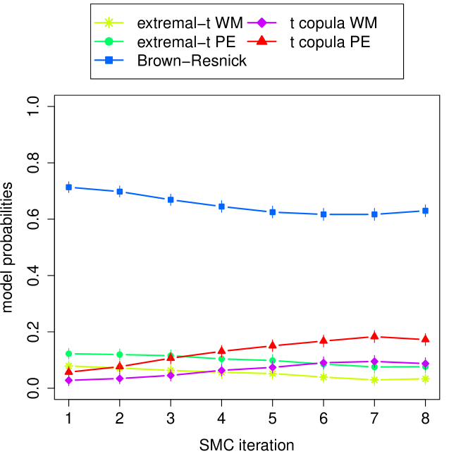
Figure 3: Progression of estimated posterior model probabilities across SMC iterations for the South Australian data set without the station in Warooka.

The estimated approximate marginal posterior distributions for the parameters of the best-fitting Brown-Resnick model are provided in Figure 4 and Table 3. For all parameters, we get posteriors that are unimodal and more informative than the respective prior distributions. Parameter estimation results for the other models are provided in Appendix F.

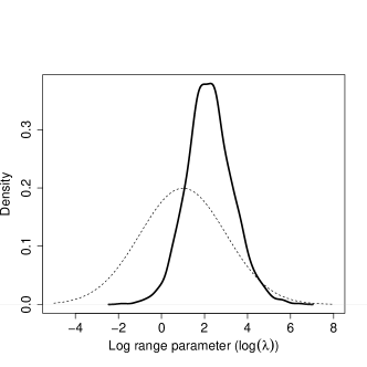
Figure 4: Solid lines: kernel density estimates of marginal posterior distributions for the best-fitting Brown-Resnick model when applied to the South Australian data set without the station in Warooka. Dashed lines: prior densities. Uniform prior densities for the smoothing and the rotation angle parameter are not displayed. However, for these parameters the abscissa range is equal to the support of the respective uniform prior distribution.

Table 3: Parameter estimates of the best-fitting Brown-Resnick model for the South Australian data set without the station in Warooka. The values of the angle $\alpha$ are given in radiants and are divided by $\pi$.

Parameter	Mean	SD	$2.5\%$ quantile	Median	$97.5\%$ quantile
$\log(\lambda)$	$2.24$	$1.08$	$0.19$	$2.19$	$4.48$
$\lambda$	$17.74$	$32.30$	$1.21$	$8.98$	$88.08$
$\kappa$	$0.51$	$0.16$	$0.20$	$0.51$	$0.82$
$\alpha/\pi$	$0.33$	$0.11$	$0.08$	$0.34$	$0.49$
$\log(r)$	$1.34$	$1.39$	$--1.28$	$1.27$	$4.33$
$r$	$10.75$	$24.71$	$0.28$	$3.55$	$76.15$

In Appendix G, the pairwise extremal coefficient functions evaluated at the median posterior parameter values are plotted for all the models.

To check the overall goodness of fit, we compare the observed pairwise F-madogram and Kendall’s $\tau$ estimates with their posterior predictive distributions. To that end, we simulated $10,\!000$ data sets from the posterior predictive distribution. Each data set (18 observations on each of 25 locations) was generated by drawing one particle with replacement from the final particle set and then simulating the data set depending on the selected particle’s model indicator and parameter values. Given this sample, we can estimate the posterior predictive distributions of all the dependence indicators for all the location pairs. Note that the final particle set contains particles from all models with an estimated posterior probability greater than $0$, so the posterior predictive distributions are the Bayesian model averages over all models.

In Figure 5, we compare the observed pairwise F-madogram (left plots) and Kendall’s $\tau$ (right plots) estimates to their posterior predictive distributions. Only one location pair falls outside the $95\%$ posterior predictive probability interval for the F-madogram. This location pair is depicted in the left bottom plot of Figure 5.

Despite excluding Warooka, our models are not able to perfectly capture the dependence structure. For high distances, the posterior predictive distribution puts too much mass on summary values that indicate high dependency, for smaller distances it puts too much mass on summary values indicating low dependency, see also the boundaries of the $95\%$ posterior predictive probability intervals in Figure 5. Due to the geography of the locations, especially the vicinity of most stations to the ocean, more complex dependence structures would have to be considered to achieve a better fit.

F-madogram	Kendall’s $\tau$

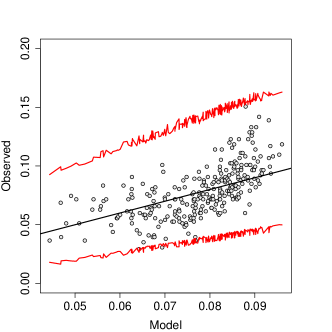
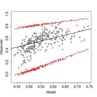
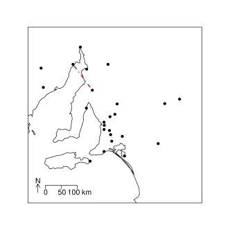
Figure 5: Top row: observed pairwise F-madogram (left) and Kendall’s $\tau$ (right) estimates vs. posterior predictive means of these estimates for each pair of locations (location ’Warooka’ is excluded). The red lines connect the $2.5\%$ and $97.5\%$ quantiles of the posterior predictive distributions for the location pairs. Bottom row: maroon dashed lines connect location pairs with unusually high observed mutual dependency. These are location pairs where the observed F-madogram estimate is below the $2.5\%$ quantile of posterior predictive distribution (left) or the observed Kendall’s $\tau$ estimate is above the $97.5\%$ quantile of posterior predictive distribution (right).

5 Discussion

The research presented in this paper expands the use of ABC for spatial extremes applications to include model selection problems. We show that the spatial dependence structure of the maximum temperature data collected around the state of South Australia is best captured by a Brown-Resnick model out of a collection of three max-stable models and two non-extremal Student-$t$ copula models. For this analysis, we exclude the station in Warooka because we consider it to be an outlier. It should be emphasised that this paper provides a case study of the application of ABC to model selection problems for spatial extremes and is not meant to be directly used to inform decision-making. The models we consider are not able to capture the intricacies of the particular environmental process in their entirety.

We would like to highlight some extensions to the straightforward geometrically anisotropic max-stable models used that would provide a more realistic representation of the spatial structure of the maximum temperature for further research. Our work has ignored any effect that might be attributable to the fact that part of the region in Figure 1 is actually a large body of water that would affect the local temperature near the coast. As such, it might be more appropriate to focus on the land mass of the region. One might determine a transformation of the land mass to a regular geometry while keeping the distance measure positive-definite by using complex spatial smoothers (Wood et al., 2008; Sangalli et al., 2013). Blanchet and Davison (2011) discuss several options to model anisotropic behaviour beyond geometric anisotropy.

All the models we consider assume unit Fréchet marginal distributions. If that is not the case, one has to transform the data properly prior to model fitting, as we did, or the number of parameters to be estimated has to be increased drastically by three GEV parameters per location. Therefore, the marginal GEV parameters are often modelled themselves by employing spatial smoothing models. This kind of modelling is required if the fitted max-stable model is used to interpolate the measurements at unobserved locations on the original measurement scale. Erhardt and Smith (2012) interpolate the GEV parameters on unobserved locations by applying Kriging. The R package SpatialExtremes (Ribatet et al., 2017) facilitates the use of P-splines for GEV response surface modelling. The shape parameter $\xi$ often exhibits little variability and follows no discernible pattern and is therefore set to a constant value over the whole space (Ribatet, 2013; Erhardt and Smith, 2012). Investigations of the appropriate modelling of the marginal GEV parameters and quantification of the corresponding uncertainty on model results are beyond the scope of this study but would be of interest in further work. There are also other models for spatial extremes that could be considered, such as those based on latent variable models (Davison et al., 2012).

In addition, there are still numerous improvement opportunities for the ABC model selection algorithm and ABC algorithms in general. Use of more sophisticated classification methods such as random forests (Pudlo et al., 2016) in the FP step could potentially provide improved performance at the expense of increased computation and less straightforward interpretations of the classification method’s direct outputs. Optimising the efficiency of the ABC algorithm is also an active research area. Such optimisations are particularly vital for applications involving computationally heavy model simulations such as the exact simulation of max-stable models on a dense grid. Methods such as Lazy ABC (Prangle, 2016) and expectation propagation ABC (Barthelmé et al., 2015) introduce additional approximations to the standard ABC method to decrease the computational time required to obtain the approximate posterior for computationally expensive models. As noted in Barthelmé et al. (2015), these methods appear promising for model selection problems as well.

Appendix A ABC algorithm summary

In the following summary of our ABC method, we have omitted the time indices for the particles and the parameter proposal distributions $q_{k}(\cdot)$ to avoid notational clutter. The two steps of our ABC method for model selection and parameter estimation are:

1. FP step
   Inputs: number of model simulations $M$ (assumed to be a multiple of $K$), $K$ candidate models, parameter prior distributions $\pi(\bm{\phi}_{k}|\mathcal{M}=k)\>(k=0,\ldots,K-1)$, choice of regression summary statistics $\bm{g}(\bm{z})$.

   1. If the model prior is uniform, draw $M/K$ parameter vectors from each candidate model’s parameter prior distribution to obtain $P=\{k^{i},\bm{\phi}_{k^{i}}^{i}\}_{i=1}^{M}$, where $\bm{\phi}_{k^{i}}^{i}\sim\pi(\bm{\phi}_{k^{i}}|\,\mathcal{M}=k^{i})$.

   2. Simulate from the respective candidate models for each element in $P$ to obtain the particle set $PP=\{k^{i},\bm{\phi}_{k^{i}}^{i},\bm{u}^{i}\}_{i=1}^{M}$, where $\bm{u}^{i}\sim f_{k^{i}}(\bm{u}|\,\bm{\phi}_{k^{i}}^{i})$. Compute the regression summary statistics $\bm{g}(\bm{u}^{i})$ for each simulated data set in $PP$.

   3. Perform a stepwise multinomial logistic regression using all $M$ particles in $PP$, where the model indicator $k^{i}$ is the outcome variable and the regression summary statistics $\bm{g}(\bm{u}^{i})$ are the covariates.

   4. Perform stepwise linear regressions for each model parameter $\phi_{k,j}$ ($k=0,\ldots,K-1$; $j=1,\ldots,Q_{k}$) using the respective $M/K$ parameter draws $\{\phi_{k^{i},j}^{i}:\>k^{i}=k\}_{i=1}^{M}$ in $PP$ as the outcome variable and the regression summary statistics $\{\bm{g}(\bm{u}^{i}):\>k^{i}=k\}_{i=1}^{M}$ as covariates.

   Outputs: regression coefficient estimates $\hat{\bm{\beta}}_{k}$ ($k=1,\ldots,K-1$) and $\hat{\bm{\beta}}_{k,j}$ ($k=0,\ldots,K-1$; $j=1,\ldots,Q_{k}$) from the logistic and linear regressions, respectively.

2. SMC ABC step
   Inputs: regression coefficient estimates from FP step, simulation size $N_{2}$ for initial ABC rejection step, number of particles $N$, SMC replenishment tuning parameters $\delta$ and $c$, observed data $\bm{z}$, discrepancy function $d_{T}[\cdot,\cdot]$, RJ-MCMC model switch proposals $q_{k,k^{*}}$, RJ-MCMC proposal distribution for model $k$’s parameters $q_{k}(\cdot)$ $(k=0,\ldots,K-1)$, stopping criteria (final tolerance $\epsilon_{\min}$ and/or minimum acceptance probability $p_{\mathrm{acc},\min}$).

   1. Generate the prior predictive draws $\{k^{i},\bm{\phi}_{k^{i}}^{i},\bm{u}^{i}\}_{i=1}^{N_{2}}$ and perform rejection ABC to obtain the initial particle set $\{k^{i},\bm{\phi}_{k^{i}}^{i},\bm{u}^{i}\}_{i=1}^{N}$.

   2. Set the acceptance probability $p_{\mathrm{acc},0}$ to a value $>p_{\mathrm{acc},\min}$ and $R_{1}$ to some arbitrary value (not too small). Set $t=1$.

   3. Denote $\epsilon_{t}$ to be the largest discrepancy value in the current particle set. If $\epsilon_{t}\leq\epsilon_{\min}$ or $p_{\mathrm{acc},t-1}\leq p_{\mathrm{acc},\min}$, terminate algorithm.

   4. Drop the $N_{\delta}=\lceil\delta N\rceil$ particles with the largest discrepancy values from the particle set. Set $\epsilon_{t}$ to be the largest discrepancy value of the remaining $N-N_{\delta}$ particles.

   5. Compute the parameters in $q_{k}(\cdot)$ using the remaining particles from model $k$.

   6. Resample $N_{\delta}$ particles with replacement from the remaining particle set until a full set of $N$ particles is recovered.

   7. To each newly resampled particle $i$ ($i=N-N_{\delta}+1,\ldots,N$), a RJ-MCMC kernel is applied $R_{t}$ times, where the kernel’s Metropolis-Hastings (MH) ratio for acceptance of a move from $(k^{i}=k,\>\bm{\phi}_{k^{i}}^{i}=\bm{\phi}_{k},\>\bm{u}^{i}=\bm{u})$ to the proposed values $(k^{i}=k^{*}\sim q_{k,k^{*}},\>\bm{\phi}_{k^{i}}^{i}=\bm{\phi}_{k^{*}}^{*}\sim q_{k^{*}}(\cdot),\>\bm{u}^{i}=\bm{u}^{*}\sim f_{k^{*}}(\cdot|\,\bm{\phi}_{k^{*}}^{*}))$ is

      $$\frac{\Pr(\mathcal{M}=k^{*})}{\Pr(\mathcal{M}=k)}\frac{\pi(\bm{\phi}_{k^{*}}^{*}|\,\mathcal{M}=k^{*})}{\pi(\bm{\phi}_{k}|\,\mathcal{M}=k)}\mathds{1}\{d_{T}[\bm{t}(\bm{z}),\bm{t}(\bm{u}^{*})]<\epsilon_{t}\}\frac{q_{k}(\bm{\phi}_{k})}{q_{k^{*}}(\bm{\phi}_{k^{*}}^{*})}\frac{q_{k^{*},k}}{q_{k,k^{*}}}$$

      and $\mathds{1}\{\cdot\}$ is the indicator function.

      When $\Pr(\mathcal{M}=k)=1/K$ and $q_{k,k^{*}}=1/K$ for all $k,k^{*}\in{1,\ldots,K}$, the model prior and model switch proposal ratios simplify to one and the MH ratio becomes

      $$\frac{\pi(\bm{\phi}_{k^{*}}^{*}|\,\mathcal{M}=k^{*})}{\pi(\bm{\phi}_{k}|\,\mathcal{M}=k)}\mathds{1}\{d_{T}[\bm{t}(\bm{z}),\bm{t}(\bm{u}^{*})]<\epsilon_{t}\}\frac{q_{k}(\bm{\phi}_{k})}{q_{k^{*}}(\bm{\phi}_{k^{*}}^{*})}.$$

   8. Compute the acceptance probability $p_{\mathrm{acc},t}=a_{t}/(R_{t}N_{\delta})$, where $a_{t}$ is the number of accepted proposals in iteration $t$, and set

      $$R_{t+1}=\left\lceil\frac{\log(c)}{\log(1-p_{\mathrm{acc},t})}\right\rceil.$$

      Increase $t$ by 1. Return to step 2(c).

   Outputs: final particle set including discrepancies $\left\{k^{i},\bm{\phi}_{k^{i}}^{i},\bm{u}^{i},d_{T}^{i}=d_{T}[\bm{t}(\bm{z}),\bm{t}(\bm{u}^{i})]\right\}_{i=1}^{N}$.

Appendix B Additional remarks and results for simulation study

B.1 Procedure to find maximum composite likelihood estimates (MCLEs)

The MCLEs were found through numerical optimisation of the pairwise log-likelihood. For some data sets and models, the result of the optimisation procedure heavily depended on the starting value. Therefore, for each data set and model we ran the optimisation routine repeatedly using random starting values from the prior distribution until we had five runs where the optimisation converged. Then we used the result from the run which led to the highest value of the objective function. For the Student-$t$ copula models, we used the MLEs found for the full log-likelihood as starting values for optimising the pairwise log-likelihood. We employed the box-constrained Broyden, Fletcher, Goldfarb, and Shanno (BFGS) quasi-Newton optimisation method, see Byrd et al. (1995).

B.2 Misclassification matrices for simulation study

B.2.1 Misclassification matrix obtained by ABC procedure

Element $(j,k)$ in the misclassification matrix below gives the probability that a data set generated from model $j$ in the simulation study is classified as being from model $k$, where the classification rule is the highest posterior model probability estimated from the final SMC particle set:

$$\blockarray{llccccc}&\Pr(1|j)\Pr(2|j)\Pr(3|j)\Pr(4|j)\Pr(5|j)\\ \block{ll[ccccc]}j=1\text{(extremal-$t$ WM)}0.380.280.210.070.07\\ j=2\text{(extremal-$t$ PE)}0.170.380.420.040.04\\ j=3\text{(Brown-Resnick)}0.040.000.960.000.00\\ j=4\text{($t$ copula WM)}0.040.040.040.440.44\\ j=5\text{($t$ copula PE)}0.000.000.000.520.48\\ .$$

B.2.2 Misclassification matrix obtained by CLIC

We compare the misclassification matrix for our simulated data sets obtained by our ABC procedure to the misclassification matrix obtained by classifying the simulated data sets according to the composite likelihood information criterion (CLIC), see, e.g., Davison et al. (2012) and Padoan et al. (2010). This is the classical criterion traditionally used for model selection of max-stable models, for which only a composite likelihood representation is available. It is a generalisation of the Akaike information criterion and accounts for the model misspecification due to using the composite likelihood.

The CLIC is defined as

$$\mathrm{CLIC}=-2\,p\ell(\tilde{\bm{\phi}}_{MCLE};\bm{z})+2\,\mathrm{tr}\left(\hat{\bm{J}}\hat{\bm{H}}^{-1}\right),$$

where $p\ell(\tilde{\bm{\phi}}_{MCLE};\bm{z})$ is the pairwise/composite log-likelihood (Equation (2.5)) evaluated at the maximum composite likelihood estimate (MCLE), $\hat{\bm{J}}$ is an estimate of $\bm{J}(\tilde{\bm{\phi}}_{MCLE})=\mathrm{Var}\left[\nabla_{\bm{\phi}}\>p\ell(\tilde{\bm{\phi}}_{MCLE};\bm{z})\right]$, and $\hat{\bm{H}}$ is an estimate of $\bm{H}(\tilde{\bm{\phi}}_{MCLE})=-\mathrm{E}\left[\nabla^{2}_{\bm{\phi}}\>p\ell(\tilde{\bm{\phi}}_{MCLE};\bm{z})\right]$. We estimate $\bm{J}$ and $\bm{H}$ as suggested in Ribatet (2013, p. 163).

In order to be able to compare all models on equal terms, we also computed the CLIC for the Student-$t$ copula models based on their pairwise likelihood representation.

Using the CLIC as classification criterion, the misclassification matrix for the simulated data sets is

$$\blockarray{llccccc}&\Pr(1|j)\Pr(2|j)\Pr(3|j)\Pr(4|j)\Pr(5|j)\\ \block{ll[ccccc]}j=1\text{(extremal-$t$ WM)}0.570.330.000.070.03\\ j=2\text{(extremal-$t$ PE)}0.370.400.030.130.07\\ j=3\text{(Brown-Resnick)}0.100.500.370.000.03\\ j=4\text{($t$ copula WM)}0.030.030.100.380.45\\ j=5\text{($t$ copula PE)}0.000.000.000.400.60\\ .$$

The inversion of $\hat{\bm{H}}$ failed sometimes. For a given data set, all models for which the inversion failed were disregarded. To assess the magnitude of the bias and the loss of information incurred by this approach, it is counted for how many models it was not possible to invert $\hat{\bm{H}}$ for each simulated data set. The table of counts across all data sets is given below:

# models where inversion failed	0	1	2	3	4	5
# simulated data sets	95	29	11	13	1	1

The aim of this section is to provide a rough comparison between the misclassification matrices of the ABC and the classical approach. We consider the quality of our CLIC-based estimate of the misclassification matrix to be sufficiently accurate for our purpose. Otherwise a more elaborate estimation technique for the CLIC would have to be employed.

Appendix C Marginal transformations to unit Fréchet

Figure 6 depicts the $25$ weather stations and the maximum likelihood estimates of the parameters of the univariate marginal generalised extreme value (GEV) distributions (location parameter $\mu$, scale parameter $\sigma$, shape parameter $\xi$). These estimates are used to transform the original data $Z^{*}_{i}(\bm{x}_{j})\sim GEV\{\mu_{j},\sigma_{j},\xi_{j}\}$, $i=1,\ldots,n$, at each station $\bm{x}_{j}$, $j=1,\ldots,H$, to unit Fréchet-scaled $Z_{i}(\bm{x}_{j})$ via the transformation

$$Z_{i}(\bm{x}_{j})=\left(1+\hat{\xi}_{j}\>\frac{Z^{*}_{i}(\bm{x}_{j})-\hat{\mu}_{j}}{\hat{\sigma}_{j}}\right)^{\frac{1}{\hat{\xi}_{j}}}.$$

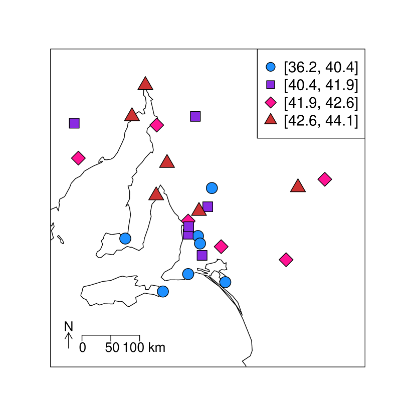
(a) GEV location parameter

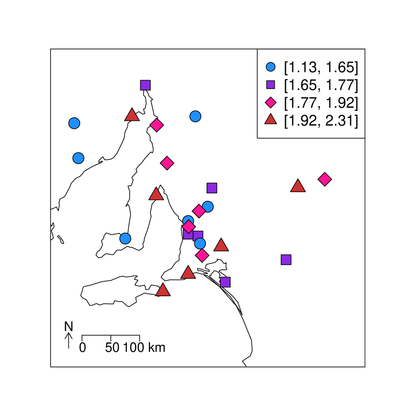
(b) GEV scale parameter

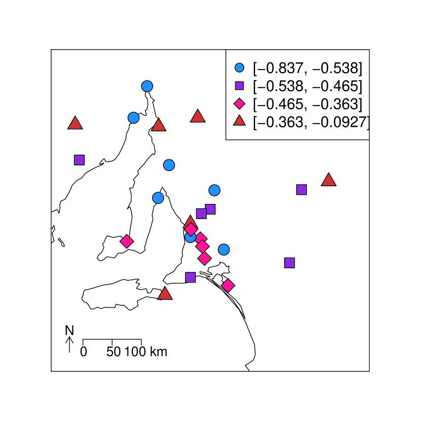
(c) GEV shape parameter

Figure 6: Colour-coded quartile sets of the three GEV parameter estimates (location $\hat{\mu}$, scale $\hat{\sigma}$, and shape $\hat{\xi}$) for the $25$ land-based weather stations around South Australia where data were collected. The quartile set with the smallest values is denoted by the blue filled circles. Sets with progressively larger values are denoted by coloured purple squares, pink diamonds and red triangles, respectively. The ranges for the quartiles are provided in the legends.

Figures 7 and 8 show the QQ plots for the transformed marginal data. For the QQ plots, the data have been transformed further to the Gumbel scale by taking the logarithms of the unit Fréchet-scaled data in order to obtain more informative plots. The p-values of the two-sided one-sample Kolmogorov-Smirnov tests of the Gumbel-scaled marginal data are also reported. The null hypothesis of Gumbel-distributed data is not rejected at all stations.

Figure 7: QQ plots of the marginal data transformed to Gumbel scale for all stations (part 1). The p-values of a two-sided one-sample Kolmogorov-Smirnov test are also reported.

Figure 8: QQ plots of the marginal data transformed to Gumbel scale for all stations (part 2). The p-values of a two-sided one-sample Kolmogorov-Smirnov test are also reported.

Appendix D Average posterior model probability matrix of FP step computed from test data

In Section 4.4, the FP step’s matrix of average posterior model probabilities is created by applying the logistic regression estimates to the training particle set, which is the particle set used to estimate the logistic regression coefficients in the first place. This may lead to overfitting. In this section, we present the average posterior model probability matrix when a separate test particle set of size $M=10,\!000$ is generated from the prior predictive distribution (with $M/5=2,\!000$ draws from each model) and the logistic regression estimates are applied to this test particle set. There are only minimal changes to the matrix reported in Section 4.4.

$$\blockarray{llccccc}&\Pr(1|j)\Pr(2|j)\Pr(3|j)\Pr(4|j)\Pr(5|j)\\ \block{ll[ccccc]}j=1\text{(extremal-$t$ WM)}0.350.340.160.090.06\\ j=2\text{(extremal-$t$ PE)}0.330.380.170.060.06\\ j=3\text{(Brown-Resnick)}0.160.150.550.070.06\\ j=4\text{($t$ copula WM)}0.090.060.060.410.37\\ j=5\text{($t$ copula PE)}0.060.060.060.370.45\\$$

Appendix E Prior predictive checks

To gauge whether the models and prior choices are appropriate for the South Australian data (when excluding Warooka), we compare the observed F-madogram and Kendall’s $\tau$ estimates for all pairs of locations with their prior predictive distributions. Figure 9 is equivalent to Figure 5, replacing draws from the posterior predictive distribution with draws from the prior predictive distribution. One draw from the prior predictive distribution is generated by choosing one of the five models with equal probability, then simulating one draw from each of the parameter priors of the chosen model (for the prior specifications see Section 4.1), and then simulating one data set from the chosen model given the parameter draws.

Figure 9 shows the observed F-madogram (left) and Kendall’s $\tau$ (right) estimates for all location pairs vs. their prior predictive means and the $95\%$ prior predictive probability intervals. The prior predictive distribution serves its purpose as a preliminary model for the observed data. The $95\%$ prior probability intervals are very wide and cover all the observed values, so the prior predictive distribution is sufficiently general and not too informative. Compared to the true data, the prior predictive distribution more strongly favours dependence indicators signalling low dependency.

F-madogram	Kendall’s $\tau$

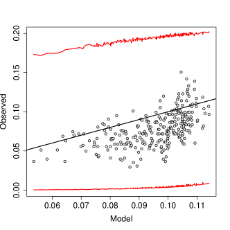
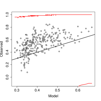
Figure 9: Observed pairwise F-madogram (left) and Kendall’s $\tau$ (right) estimates vs. prior predictive means of these estimates for each pair of locations (location ’Warooka’ is excluded). The red lines connect the $2.5\%$ and $97.5\%$ quantiles of the prior predictive distributions for the location pairs.

Appendix F Posterior distributions

Figures 10, 11, 12, and 13 show the posterior distributions of the parameters of the extremal-$t$ models with the Whittle-Matérn and powered exponential correlation function and the Student-$t$ copula models with the Whittle-Matérn and powered exponential correlation function, respectively, when the station in Warooka is excluded. These models do not have very high posterior model probabilities. For example, the estimated posterior model probability of the extremal-$t$ model with Whittle-Matérn correlation function is $3.4\%$ (67 out of 2000 particles) after the final SMC ABC iteration. Since this is a rather small sample size, the Monte Carlo error of the reported posterior estimates is high. If preciser estimates of the posterior distributions are desired for any of these models, one can run the sequential Monte Carlo ABC algorithm (or any other ABC algorithm) once more exclusively for the particular model of interest with the focus solely on parameter estimation.

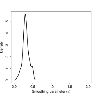
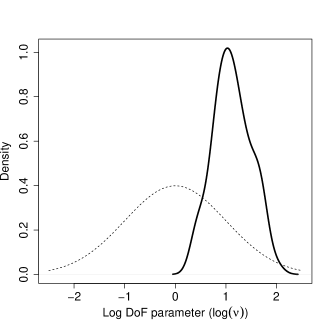
Figure 10: Solid lines: kernel density estimates of marginal posterior distributions for the extremal-$t$ model with Whittle-Matérn correlation function when applied to the South Australian data set without the station in Warooka, based on 67 particles. Dashed lines: prior densities. Uniform prior densities for the smoothing and the rotation angle parameter are not displayed. However, for these parameters the abscissa range is equal to the support of the respective uniform prior distribution.

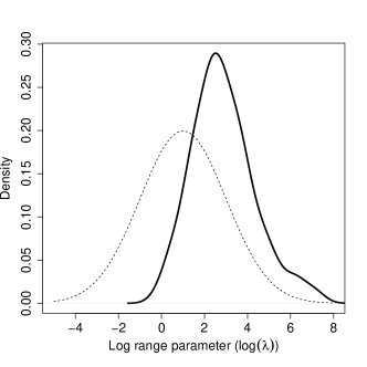
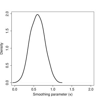
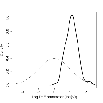
Figure 11: Solid lines: kernel density estimates of marginal posterior distributions for the extremal-$t$ model with powered exponential correlation function when applied to the South Australian data set without the station in Warooka, based on 153 particles. Dashed lines: prior densities. Uniform prior densities for the smoothing and the rotation angle parameter are not displayed. However, for these parameters the abscissa range is equal to the support of the respective uniform prior distribution.

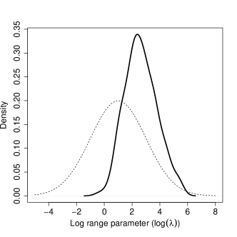
Figure 12: Solid lines: kernel density estimates of marginal posterior distributions for the Student-$t$ copula model with Whittle-Matérn correlation function when applied to the South Australian data set without the station in Warooka, based on 175 particles. Dashed lines: prior densities. Uniform prior densities for the smoothing and the rotation angle parameter are not displayed. However, for these parameters the abscissa range is equal to the support of the respective uniform prior distribution.

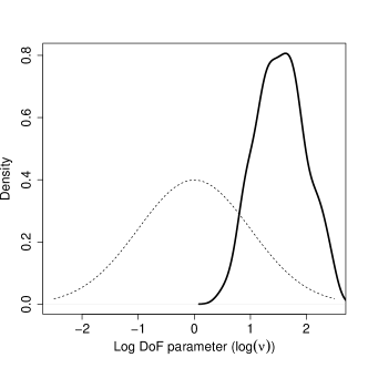
Figure 13: Solid lines: kernel density estimates of marginal posterior distributions for the Student-$t$ copula model with powered exponential correlation function when applied to the South Australian data set without the station in Warooka, based on 345 particles. Dashed lines: prior densities. Uniform prior densities for the smoothing and the rotation angle parameter are not displayed. However, for these parameters the abscissa range is equal to the support of the respective uniform prior distribution.

Appendix G Extremal coefficient function plots

A common graphical goodness-of-fit check of spatial max-stable models is to visually assess how well the theoretical pairwise extremal coefficient curve as a function of the distance between the locations fits the cloud of observed pairwise extremal coefficients. Since for our models the distances depend on the parameters governing the geometric anisotropy, we have to assume a specific parameter configuration to compute the interpoint distances for all the points in the cloud. Different anisotropy parameters give rise to different clouds of observed extremal coefficients. For each model, we will set the parameter values to their respective posterior median values.

Specifically, we compute the distance between locations $\bm{x}_{1}$ and $\bm{x}_{2}$ as

$$h(\bm{x}_{1},\bm{x}_{2})=\frac{\|\tilde{\bm{A}}(\bm{x}_{1}-\bm{x}_{2})\|}{\tilde{\lambda}},$$

where the anisotropy matrix is

$$\tilde{\bm{A}}=\begin{pmatrix}1&0\\ 0&1/\tilde{r}\end{pmatrix}\cdot\begin{pmatrix}\cos\tilde{\alpha}&\sin\tilde{\alpha}\\ -\sin\tilde{\alpha}&\cos\tilde{\alpha}\end{pmatrix},$$

and $\tilde{\lambda}$, $\tilde{\alpha}$, and $\tilde{r}$ are the posterior medians of the range, rotation angle, and principal axes ratio parameters, respectively. That is, we transform the location space to $\tilde{\mathcal{X}}=\left(\tilde{\bm{A}}/\tilde{\lambda}\right)\mathcal{X}$ and compute the Euclidean distances in this transformed space.

For these transformed distances $h$, the theoretical extremal coefficient curve of the Brown-Resnick model with power variogram evaluated at the posterior median of the smoothness parameter, $\tilde{\kappa}$, is given by (Davison et al., 2012)

$$\theta(h;\tilde{\kappa})=2\,\Phi\left\{a(h;\tilde{\kappa})/2\right\},$$

where $\Phi\{\cdot\}$ is the CDF of the standard normal distribution and

$$a(h;\tilde{\kappa})=\sqrt{2h^{\tilde{\kappa}}}.$$

For the extremal-$t$ model, we have (Davison et al., 2012)

$$\theta(h;\tilde{\nu},\tilde{\kappa})=2\,T_{1;\tilde{\nu}+1}\left\{\sqrt{(\tilde{\nu}+1)\>\frac{1-\rho(h;\tilde{\kappa})}{1+\rho(h;\tilde{\kappa})}}\right\},$$

where $T_{1;\tilde{\nu}+1}\{\cdot\}$ denotes the central Student-$t$ CDF with $\tilde{\nu}+1$ degrees of freedom, $\rho(h;\tilde{\kappa})$ is one of the correlation functions described in Appendix K, $\tilde{\nu}$ is the posterior median of the degrees of freedom parameter, and $\tilde{\kappa}$ is the posterior median of the smoothness parameter.

As discussed in Section 2.3, the extremal coefficient is not defined for the Student-$t$ copula models. We can nevertheless use Equation (2.4) to generate meaningful summary statistics measuring dependence. However, no theoretical extremal coefficient curve is available and the functional form of the underlying coefficient to which the estimates converge is unknown. Therefore, we have to estimate the underlying coefficient for a given set of parameters $\tilde{\kappa}$ and $\tilde{\nu}$ at any distance $h$. For a given distance $h$, we obtain the estimate by computing Equation (2.4) for a sample of size $500,\!000$ generated from a bivariate $t$ copula model with distance $h$. To allow for a concise description of the results, we denote the underlying coefficient to which the estimates converge by extremal coefficient in accordance with the max-stable models.

Figure 14 shows the extremal coefficient function plots for all models when the station in Warooka is excluded, one plot for each model. The extremal-$t$ models fail to capture the extremal coefficients at low and medium distances, where most of the points are concentrated. The Brown-Resnick model, on the other hand, does not capture the extremal coefficients at large distances very well, but it provides the best fit for small and medium distances. The $t$ copula models also provide an adequate fit.

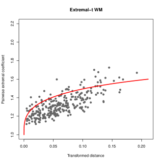
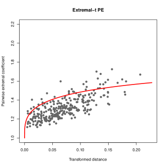
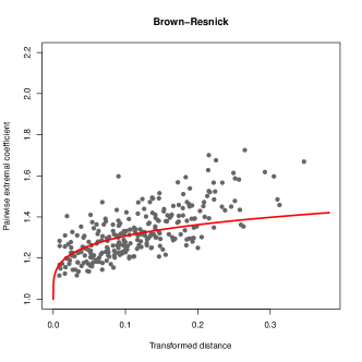
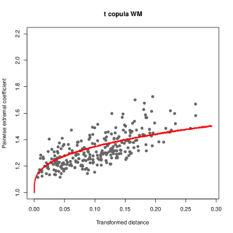
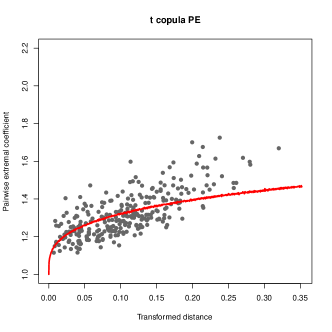
Figure 14: Extremal coefficient function plots when excluding Warooka for the extremal-$t$ model (top) with Whittle-Matérn (top left) and powered exponential (top right) correlation function, the Brown-Resnick model (middle), and the $t$ copula model (bottom) with Whittle-Matérn (bottom left) and powered exponential (bottom right) correlation function. Each plot was generated using the posterior median values of the respective model’s parameters.

Appendix H Analysis when including Warooka station

In this section, we present the results of our ABC analysis when the station in Warooka is included.

The progression of estimated posterior model probabilities is depicted in Figure 15. By including Warooka, the estimated posterior model probabilities change significantly. When Warooka is included, the posterior model probability of the Brown-Resnick model is $40\%$ at the final SMC iteration. When Warooka is excluded, this probability is $63\%$. On the other hand, the posterior model probabilities of the $t$ copula models rise to $33\%$ (powered exponential correlation function) and $20\%$ (Whittle-Matérn correlation function), so the $t$ copula models have a higher combined posterior model probability than the Brown-Resnick model. The posterior model probabilities of the extremal-$t$ models remain low.

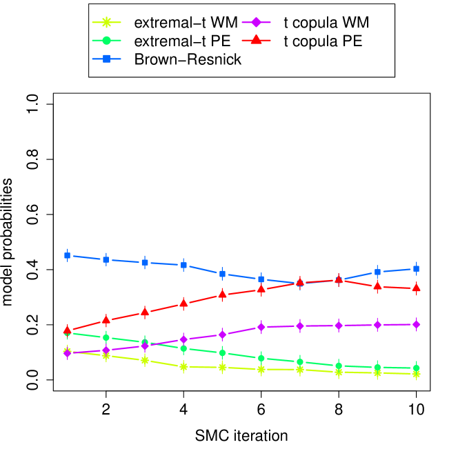
Figure 15: Progression of estimated posterior model probabilities across SMC iterations for the South Australian data set when the station in Warooka is included.

The marginal posterior distributions for the two most probable models are depicted in Figure 16 (Brown-Resnick model) and Figure 17 ($t$ copula model with powered exponential correlation function). They are mostly similar to the posterior distributions when Warooka is excluded (cf. Figures 4 and 13). However, the posterior distributions for the principal axes ratio, /, put more mass on very high values. (Note that the densities of the logarithms are plotted.) The posterior distributions for the rotation angle are more concentrated on the upper half. On the other hand, the posterior distribution for the $t$ copula model’s degrees of freedom parameter $\nu$ is slightly shifted to the left.

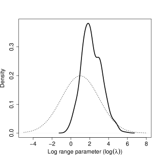
Figure 16: Solid lines: kernel density estimates of marginal posterior distributions for the Brown-Resnick model when applied to the South Australian data set including the station in Warooka. Dashed lines: prior densities. Uniform prior densities for the smoothing and the rotation angle parameter are not displayed. However, for these parameters the abscissa range is equal to the support of the respective uniform prior distribution.

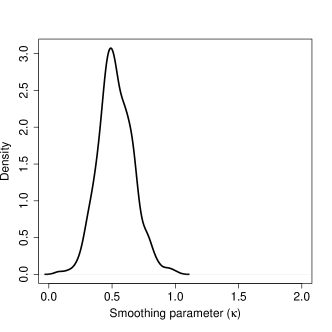
Figure 17: Solid lines: kernel density estimates of marginal posterior distributions for the $t$ copula model with powered exponential correlation function when applied to the South Australian data set including the station in Warooka. Dashed lines: prior densities. Uniform prior densities for the smoothing and the rotation angle parameter are not displayed. However, for these parameters the abscissa range is equal to the support of the respective uniform prior distribution.

The extremal coefficient function plots are displayed in Figure 18. The pattern is similar to Figure 14.

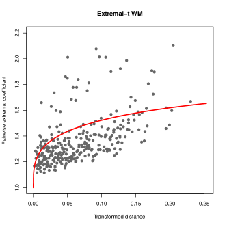
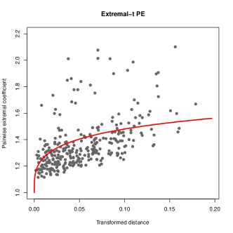
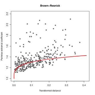
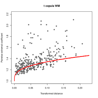
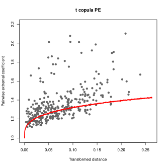
Figure 18: Extremal coefficient function plots when including Warooka for the extremal-$t$ model (top) with Whittle-Matérn (top left) and powered exponential (top right) correlation function, the Brown-Resnick model (middle), and the $t$ copula model (bottom) with Whittle-Matérn (bottom left) and powered exponential (bottom right) correlation function. Each plot was generated using the posterior median values of the respective model’s parameters.

Figure 19 shows the posterior predictive analysis for the pairwise F-madogram and Kendall’s $\tau$ estimates when Warooka is included. For $8\%$/$7\%$ of the location pairs, the observed F-madogram/ Kendall’s $\tau$ estimate falls outside the $95\%$ posterior predictive probability interval. The bottom plots in Figure 19 connect the locations in these pairs with lines. All of the outlying location pairs have an unusually low observed mutual dependency and Warooka on the peninsula is included in all of them but one. Therefore, we consider the observations collected at Warooka as being outlying observations according to our models.

F-madogram	Kendall’s $\tau$

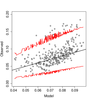
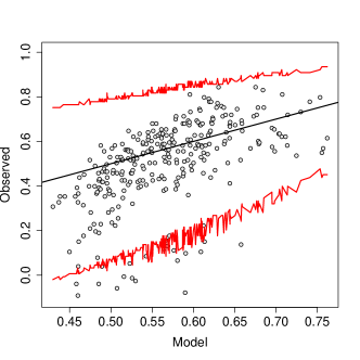
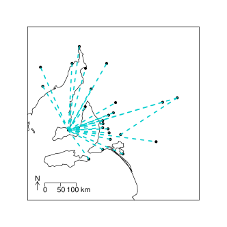
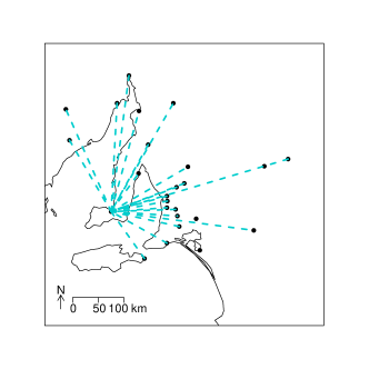
Figure 19: Top row: observed pairwise F-madogram (left) and Kendall’s $\tau$ (right) estimates vs. posterior predictive means of these estimates for each pair of locations (location ’Warooka’ is included). The red lines connect the $2.5\%$ and $97.5\%$ quantiles of the posterior predictive distributions for the location pairs. Bottom row: cyan dashed lines connect location pairs with unusually low observed mutual dependency. These are location pairs where the observed F-madogram estimate is above the $97.5\%$ quantile of posterior predictive distribution (left) or the observed Kendall’s $\tau$ estimate is below the $2.5\%$ quantile of posterior predictive distribution (right).

Appendix I Derivations of bivariate log-likelihoods

For all max-stable process models, the bivariate cumulative distribution function (CDF) is equal to

$$F(z_{1},z_{2})=\exp\left\{-V(z_{1},z_{2})\right\},$$

where $V(z_{1},z_{2})$ is called the exponent measure (see Davison et al. (2012)). The probability density function (PDF) is obtained by calculating the mixed partial derivative of $F$ w.r.t. $z_{1}$ and $z_{2}$. To shorten notation, we write $\displaystyle V_{1}(z_{1},z_{2})=\frac{\partial}{\partial z_{1}}V(z_{1},z_{2})$, $\displaystyle V_{2}(z_{1},z_{2})=\frac{\partial}{\partial z_{2}}V(z_{1},z_{2})$, and $\displaystyle V_{1,2}(z_{1},z_{2})=\frac{\partial^{2}}{\partial z_{1}\partial z_{2}}V(z_{1},z_{2})$. We obtain

$$f(z_{1},z_{2})=\exp\left\{-V(z_{1},z_{2})\right\}\left[V_{1}(z_{1},z_{2})\cdot V_{2}(z_{1},z_{2})-V_{1,2}(z_{1},z_{2})\right],$$

and so the log-likelihood is

$$\ell(z_{1},z_{2})=\log f(z_{1},z_{2})=-V(z_{1},z_{2})+\log\left[V_{1}(z_{1},z_{2})\cdot V_{2}(z_{1},z_{2})-V_{1,2}(z_{1},z_{2})\right].$$ (I.1)

I.1 Brown-Resnick model

The bivariate CDF of the Brown-Resnick model with power variogram has the form (Ribatet, 2013)

$$F(z_{1},z_{2}) = \exp\biggl{\{}-\frac{1}{z_{1}}\Phi\left[\frac{a(\bm{x}_{1},\bm{x}_{2};\bm{\phi})}{2}+\frac{1}{a(\bm{x}_{1},\bm{x}_{2};\bm{\phi})}\log\frac{z_{2}}{z_{1}}\right]$$

$$\phantom{\exp\Biggl{\{}}-\frac{1}{z_{2}}\Phi\left[\frac{a(\bm{x}_{1},\bm{x}_{2};\bm{\phi})}{2}+\frac{1}{a(\bm{x}_{1},\bm{x}_{2};\bm{\phi})}\log\frac{z_{1}}{z_{2}}\right]\biggr{\}},$$

where $\Phi(\cdot)$ denotes the standard normal CDF,

$$a(\bm{x}_{1},\bm{x}_{2};\bm{\phi}=(\lambda,\kappa,\alpha,)/)=\sqrt{2\,h(\bm{x}_{1},\bm{x}_{2};\bm{\phi}\backslash\{\kappa\})^{\kappa}},$$

and the distance function is

$$h(\bm{x}_{1},\bm{x}_{2};\lambda,\alpha,)/=\frac{\|\bm{A}(\bm{x}_{1}-\bm{x}_{2})\|}{\lambda},$$

with anisotropy matrix

$$\bm{A}=\begin{pmatrix}1&0\\ 0&1/r\end{pmatrix}\cdot\begin{pmatrix}\cos\alpha&\sin\alpha\\ -\sin\alpha&\cos\alpha\end{pmatrix}.$$

There are four parameters in this model, the range parameter, $\lambda>0$, the smoothing parameter, $0<\kappa\leq 2$, the counter-clockwise rotation angle of the confidence ellipse, $0\leq\alpha<\pi/2$, and the ratio of the principal axes of the confidence ellipse, $>/0$.

Therefore, the exponent measure is

$$V(z_{1},z_{2})=\frac{1}{z_{1}}\Phi\left[\frac{a(\bm{x}_{1},\bm{x}_{2};\bm{\phi})}{2}+\frac{1}{a(\bm{x}_{1},\bm{x}_{2};\bm{\phi})}\log\frac{z_{2}}{z_{1}}\right]+\frac{1}{z_{2}}\Phi\left[\frac{a(\bm{x}_{1},\bm{x}_{2};\bm{\phi})}{2}+\frac{1}{a(\bm{x}_{1},\bm{x}_{2};\bm{\phi})}\log\frac{z_{1}}{z_{2}}\right].$$ (I.2)

The partial derivatives of the exponent measure are given in Padoan et al. (2010, p. 275). Setting $\displaystyle w(z_{1},z_{2};\bm{\phi})=\frac{a(\bm{x}_{1},\bm{x}_{2};\bm{\phi})}{2}+\frac{1}{a(\bm{x}_{1},\bm{x}_{2};\bm{\phi})}\log\frac{z_{2}}{z_{1}}$ and $v(z_{1},z_{2};\bm{\phi})=a(\bm{x}_{1},\bm{x}_{2};\bm{\phi})-w(z_{1},z_{2};\bm{\phi})$, and writing $v$, $w$, and $a$ without arguments for brevity, the partial derivatives are

$$V_{1}(z_{1},z_{2})=\frac{\varphi(v)}{az_{1}z_{2}}-\frac{\varphi(w)}{az_{1}^{2}}-\frac{\Phi(w)}{z_{1}^{2}},$$ (I.3)

$$V_{2}(z_{1},z_{2})=\frac{\varphi(w)}{az_{1}z_{2}}-\frac{\varphi(v)}{az_{2}^{2}}-\frac{\Phi(v)}{z_{2}^{2}},$$ (I.4)

and

$$V_{1,2}(z_{1},z_{2})=-\frac{v\varphi(w)}{a^{2}z_{1}^{2}z_{2}}-\frac{w\varphi(v)}{a^{2}z_{1}z_{2}^{2}},$$ (I.5)

where $\varphi(\cdot)$ denotes the standard normal PDF.

I.2 Extremal-$t$ model

The bivariate CDF for the extremal-$t$ model is (Ribatet, 2013)

$$F(z_{1},z_{2}) = \exp\biggl{\{}-\frac{1}{z_{1}}T_{1;\nu+1}\left[a(\bm{x}_{1},\bm{x}_{2};\bm{\phi},\nu)\left\{q(z_{1},z_{2};\nu)-\rho(\bm{x}_{1},\bm{x}_{2};\bm{\phi})\right\}\right]$$

$$\phantom{\exp\bigl{\{}}-\frac{1}{z_{2}}T_{1;\nu+1}\left[a(\bm{x}_{1},\bm{x}_{2};\bm{\phi},\nu)\left\{r(z_{1},z_{2};\nu)-\rho(\bm{x}_{1},\bm{x}_{2};\bm{\phi})\right\}\right]\biggr{\}},$$

where $T_{1;\nu+1}$ denotes the CDF of a univariate Student-$t$ distribution with $\nu+1$ degrees of freedom,

$$a(\bm{x}_{1},\bm{x}_{2};\bm{\phi},\nu)=\sqrt{\frac{\nu+1}{1-\rho(\bm{x}_{1},\bm{x}_{2};\bm{\phi})^{2}}},$$

$$q(z_{1},z_{2};\nu)=\left(\frac{z_{2}}{z_{1}}\right)^{1/\nu},$$

$$r(z_{1},z_{2};\nu)=1/q(z_{1},z_{2};\nu)=\left(\frac{z_{1}}{z_{2}}\right)^{1/\nu},$$

and $\rho(\bm{x}_{1},\bm{x}_{2};\bm{\phi})$ is one of the correlation functions given in Appendix K.

Therefore, the exponent measure is

$$V(z_{1},z_{2}) = \phantom{+}\frac{1}{z_{1}}T_{1;\nu+1}\left[a(\bm{x}_{1},\bm{x}_{2};\bm{\phi},\nu)\left\{q(z_{1},z_{2};\nu)-\rho(\bm{x}_{1},\bm{x}_{2};\bm{\phi})\right\}\right]$$ (I.6)

$$+\frac{1}{z_{2}}T_{1;\nu+1}\left[a(\bm{x}_{1},\bm{x}_{2};\bm{\phi},\nu)\left\{r(z_{1},z_{2};\nu)-\rho(\bm{x}_{1},\bm{x}_{2};\bm{\phi})\right\}\right].$$

To save space, let us introduce the functions

$$w(z_{1},z_{2};\bm{\phi},\nu)=a(\bm{x}_{1},\bm{x}_{2};\bm{\phi},\nu)\left\{q(z_{1},z_{2};\nu)-\rho(\bm{x}_{1},\bm{x}_{2};\bm{\phi})\right\}$$

and

$$v(z_{1},z_{2};\bm{\phi},\nu)=a(\bm{x}_{1},\bm{x}_{2};\bm{\phi},\nu)\left\{r(z_{1},z_{2};\nu)-\rho(\bm{x}_{1},\bm{x}_{2};\bm{\phi})\right\}.$$

To shorten notation, we will suppress the arguments in $a(\cdot)$, $q(\cdot)$, $r(\cdot)$, $\rho(\cdot)$, $w(\cdot)$, and $v(\cdot)$. However, one should always be aware of which variables and parameters they depend upon.

Using the facts that $\displaystyle\frac{\partial w}{\partial z_{1}}=-\frac{a}{\nu z_{1}}q$, $\displaystyle\frac{\partial w}{\partial z_{2}}=\frac{a}{\nu z_{2}}q$, $\displaystyle\frac{\partial v}{\partial z_{1}}=\frac{a}{\nu z_{1}}r$ and $\displaystyle\frac{\partial v}{\partial z_{2}}=-\frac{a}{\nu z_{2}}r$, it is straightforward to derive the partial derivatives of $V(z_{1},z_{2})$:

$$V_{1}(z_{1},z_{2})=-\frac{1}{z_{1}^{2}}T_{1;\nu+1}(w)-\frac{aq}{\nu z_{1}^{2}}t_{1;\nu+1}(w)+\frac{ar}{\nu z_{1}z_{2}}t_{1;\nu+1}(v),$$ (I.7)

$$V_{2}(z_{1},z_{2})=-\frac{1}{z_{2}^{2}}T_{1;\nu+1}(v)-\frac{ar}{\nu z_{2}^{2}}t_{1;\nu+1}(v)+\frac{aq}{\nu z_{1}z_{2}}t_{1;\nu+1}(w),$$ (I.8)

and

$$V_{1,2}(z_{1},z_{2}) = -\frac{(\nu+1)aq}{\nu^{2}z_{1}^{2}z_{2}}t_{1;\nu+1}(w)-\frac{a^{2}q^{2}}{\nu^{2}z_{1}^{2}z_{2}}\frac{\partial t_{1;\nu+1}(w)}{\partial w}$$ (I.9)

$$-\frac{(\nu+1)ar}{\nu^{2}z_{1}z_{2}^{2}}t_{1;\nu+1}(v)-\frac{a^{2}r^{2}}{\nu^{2}z_{1}z_{2}^{2}}\frac{\partial t_{1;\nu+1}(v)}{\partial v},$$

where $t_{1;\nu+1}(x)$ denotes the PDF of the univariate Student-$t$ distribution with $\nu+1$ degrees of freedom and

$$\frac{\partial t_{1;\nu+1}(x)}{\partial x}=-\frac{x(\nu+2)}{x^{2}+\nu+1}\;t_{1;\nu+1}(x).$$

I.3 Student-$t$ copula model

The $H$-dimensional marginal CDF for the $t$ copula model with unit Fréchet margins is (Demarta and McNeil, 2005)

$$F(z_{1},\ldots,z_{H})=T_{H;\nu}\left\{T_{1;\nu}^{-1}[G(z_{1})],\ldots,T_{1;\nu}^{-1}[G(z_{H})];\>\bm{\Sigma}(\bm{x}_{1},\ldots,\bm{x}_{H};\bm{\phi})\right\},$$

where $G(z)=\exp(-1/z)$ is the CDF of the unit Fréchet distribution, $T_{1;\nu}^{-1}[\cdot]$ is the inverse CDF (quantile function) of the univariate central Student-$t$ distribution with $\nu$ degrees of freedom, and $T_{H;\nu}\{\cdots;\>\bm{\Sigma}(\bm{x}_{1},\ldots,\bm{x}_{H};\bm{\phi})\}$ denotes the CDF of the $H$-dimensional central Student-$t$ distribution with $\nu$ degrees of freedom and dispersion matrix

$$\bm{\Sigma}(\bm{x}_{1},\ldots,\bm{x}_{H};\bm{\phi})=\begin{pmatrix}1&\rho(\bm{x}_{1},\bm{x}_{2};\bm{\phi})&\cdots&\rho(\bm{x}_{1},\bm{x}_{H};\bm{\phi})\\ \rho(\bm{x}_{2},\bm{x}_{1};\bm{\phi})&1&\cdots&\rho(\bm{x}_{2},\bm{x}_{H};\bm{\phi})\\ \vdots&\vdots&\ddots&\vdots\\ \rho(\bm{x}_{H},\bm{x}_{1};\bm{\phi})&\rho(\bm{x}_{H},\bm{x}_{2};\bm{\phi})&\cdots&1\end{pmatrix},$$

where $\rho(\cdot,\cdot;\bm{\phi})$ is one of the correlation functions given in Appendix K.

Therefore, the log-likelihood of this model is

$$\ell(z_{1},\ldots,z_{H}) = \phantom{-}\log t_{H;\nu}\left\{T_{1;\nu}^{-1}[G(z_{1})],\ldots,T_{1;\nu}^{-1}[G(z_{H})];\>\bm{\Sigma}(\bm{x}_{1},\ldots,\bm{x}_{H};\bm{\phi})\right\}$$ (I.10)

$$-\sum_{i=1}^{H}\left[\log t_{1;\nu}\left\{T_{1;\nu}^{-1}[G(z_{i})]\right\}-\log g(z_{i})\right],$$

where

$$t_{H;\nu}\left\{y_{1},\ldots,y_{H};\>\bm{\Sigma}\right\}=\frac{\Gamma\{(\nu+H)/2\}}{\Gamma\{\nu/2\}(\nu\pi)^{H/2}\,|\bm{\Sigma}|^{1/2}}\left\{1+\frac{1}{\nu}\left((y_{1},\ldots,y_{H})\,\bm{\Sigma}^{-1}\begin{pmatrix}y_{1}\\ \vdots\\ y_{H}\end{pmatrix}\right)\right\}^{-(\nu+H)/2}$$ (I.11)

is the PDF of the $H$-dimensional central Student-$t$ distribution with $\nu$ degrees of freedom and dispersion matrix $\bm{\Sigma}$,

$$t_{1;\nu}\{y\}=\frac{\Gamma\{(\nu+1)/2\}}{\sqrt{\nu\pi}\,\Gamma\{\nu/2\}}\left\{1+\frac{y^{2}}{\nu}\right\}^{-(\nu+1)/2}$$ (I.12)

is the PDF of the univariate central Student-$t$ distribution with $\nu$ degrees of freedom, and

$$g(z)=\frac{\exp(-1/z)}{z^{2}}$$

is the PDF of the unit Fréchet distribution.

In the bivariate case, we can simplify Equation (I.10) further. Plugging the PDFs (I.11) and (I.12) into Equation (I.10) for $H=2$ and simplifying the notation by introducing $\eta_{1}=T_{1;\nu}^{-1}[G(z_{1})]$ and $\eta_{2}=T_{1;\nu}^{-1}[G(z_{2})]$ and omitting the arguments of $\rho(\bm{x}_{1},\bm{x}_{2};\bm{\phi})$ yields

$$\ell(z_{1},z_{2}) = \phantom{-}\log(\nu/2)-\frac{1}{2}\log(1-\rho^{2})-\frac{\nu+2}{2}\log\left[1+\frac{\eta_{1}^{2}-2\rho\eta_{1}\eta_{2}+\eta_{2}^{2}}{\nu(1-\rho^{2})}\right]$$ (I.13)

$$-2\log\Gamma\{(\nu+1)/2\}+2\log\Gamma\{\nu/2\}+\frac{\nu+1}{2}\left[\log\left(1+\frac{\eta_{1}^{2}}{\nu}\right)+\log\left(1+\frac{\eta_{2}^{2}}{\nu}\right)\right]$$

$$-1/z_{1}-2\log(z_{1})-1/z_{2}-2\log(z_{2}).$$

Appendix J Partial derivatives of log-likelihood functions w.r.t. parameters

Next we compute the partial derivatives of the log-likelihood function w.r.t. the parameters of the model (usually correlation parameters). For now, we do not explicitly specify the form of the correlation function $\rho(\cdot,\cdot;\bm{\phi})$ or of the function $a(\cdot,\cdot;\bm{\phi})$ in the Brown-Resnick model. The partial derivatives of specific correlation functions $\rho(\cdot,\cdot;\bm{\phi})$ and of the Brown-Resnick model’s function $a(\cdot,\cdot;\bm{\phi})$ with respect to each of their parameters are given in Appendix K.

Similar to Appendix I, when considering the partial derivative of the log-likelihood w.r.t. some generic parameter $\phi_{i}\in\bm{\phi}$, we write $\displaystyle V_{i}(z_{1},z_{2};\bm{\phi})=\frac{\partial}{\partial\phi_{i}}V(z_{1},z_{2};\bm{\phi})$, $\displaystyle V_{1,i}(z_{1},z_{2};\bm{\phi})=\frac{\partial}{\partial\phi_{i}}V_{1}(z_{1},z_{2};\bm{\phi})$, $\displaystyle V_{2,i}(z_{1},z_{2};\bm{\phi})=\frac{\partial}{\partial\phi_{i}}V_{2}(z_{1},z_{2};\bm{\phi})$, and $\displaystyle V_{1,2,i}(z_{1},z_{2};\bm{\phi})=\frac{\partial}{\partial\phi_{i}}V_{1,2}(z_{1},z_{2};\bm{\phi})$.

Setting $D(z_{1},z_{2};\bm{\phi})=V_{1}(z_{1},z_{2};\bm{\phi})\cdot V_{2}(z_{1},z_{2};\bm{\phi})-V_{1,2}(z_{1},z_{2};\bm{\phi})$, the derivative of the log-likelihood function (I.1) w.r.t. the generic parameter $\phi_{i}$ is

$$\frac{\partial}{\partial\phi_{i}}\ell(z_{1},z_{2};\bm{\phi}) = -V_{i}(z_{1},z_{2};\bm{\phi})+\frac{1}{D(z_{1},z_{2};\bm{\phi})}\bigl{[}V_{1,i}(z_{1},z_{2};\bm{\phi})\cdot V_{2}(z_{1},z_{2};\bm{\phi})$$

$$\phantom{-V_{i}(z_{1},z_{2};\bm{\phi})+}+V_{1}(z_{1},z_{2};\bm{\phi})\cdot V_{2,i}(z_{1},z_{2};\bm{\phi})-V_{1,2,i}(z_{1},z_{2};\bm{\phi})\bigr{]}.$$

J.1 Brown-Resnick model

To obtain $V_{i}(z_{1},z_{2};\bm{\phi})$, $V_{1,i}(z_{1},z_{2};\bm{\phi})$, $V_{2,i}(z_{1},z_{2};\bm{\phi})$, and $V_{1,2,i}(z_{1},z_{2};\bm{\phi})$ for the Brown-Resnick model, we need to compute the partial derivatives of Equations (I.2), (I.3), (I.4), and (I.5), respectively, w.r.t. $\phi_{i}$. These formulae are given in Padoan et al. (2010, p. 275–276). Using the same notation and abbreviations as in Appendix I.1, they are given by

$$V_{i}(z_{1},z_{2};\bm{\phi})=\left[\frac{v\varphi(w)}{az_{1}}+\frac{w\varphi(v)}{az_{2}}\right]\frac{\partial a}{\partial\phi_{i}},$$

$$V_{1,i}(z_{1},z_{2};\bm{\phi})=\left[\frac{(1-v^{2})\varphi(w)}{a^{2}z_{1}^{2}}-\frac{(1+wv)\varphi(v)}{a^{2}z_{1}z_{2}}\right]\frac{\partial a}{\partial\phi_{i}},$$

$$V_{2,i}(z_{1},z_{2};\bm{\phi})=\left[\frac{(1-w^{2})\varphi(v)}{a^{2}z_{2}^{2}}-\frac{(1+wv)\varphi(w)}{a^{2}z_{1}z_{2}}\right]\frac{\partial a}{\partial\phi_{i}},$$

and

$$V_{1,2,i}(z_{1},z_{2};\bm{\phi})=\frac{(wv^{2}+2v-w)\varphi(w)z_{2}+(vw^{2}+2w-v)\varphi(v)z_{1}}{a^{3}z_{1}^{2}z_{2}^{2}}\frac{\partial a}{\partial\phi_{i}}.$$

J.2 Extremal-$t$ model

On the one hand, we have to compute $V_{\nu}(z_{1},z_{2};\bm{\phi},\nu)$, $V_{1,\nu}(z_{1},z_{2};\bm{\phi},\nu)$, $V_{2,\nu}(z_{1},z_{2};\bm{\phi},\nu)$, and $V_{1,2,\nu}(z_{1},z_{2};\bm{\phi},\nu)$, the partial derivatives w.r.t. the degrees of freedom parameter $\nu$. On the other hand, we need the partial derivatives w.r.t. any of the generic correlation parameters $\phi_{i}$, $V_{i}(z_{1},z_{2};\bm{\phi},\nu)$, $V_{1,i}(z_{1},z_{2};\bm{\phi},\nu)$, $V_{2,i}(z_{1},z_{2};\bm{\phi},\nu)$, and $V_{1,2,i}(z_{1},z_{2};\bm{\phi},\nu)$. Both set of derivatives are based on the formulae (I.6), (I.7), (I.8), and (I.9).

Let us start with the partial derivatives w.r.t. $\nu$. Before giving these, we calculate some useful quantities that we will need. As in Appendix I.2, we will generally omit any arguments to keep the notation short.

$$\frac{\partial a}{\partial\nu} = \frac{a}{2(\nu+1)},$$

$$\frac{\partial q}{\partial\nu} = -\frac{q\log q}{\nu},$$

$$\frac{\partial r}{\partial\nu} = -\frac{r\log r}{\nu},$$

$$\frac{\partial w}{\partial\nu} = (q-\rho)\frac{\partial a}{\partial\nu}+a\frac{\partial q}{\partial\nu},$$

$$\frac{\partial v}{\partial\nu} = (r-\rho)\frac{\partial a}{\partial\nu}+a\frac{\partial r}{\partial\nu}.$$

We will also need the derivatives of the CDF and PDF of a univariate Student-$t$ distribution with $\nu+1$ degrees of freedom w.r.t. $\nu$ evaluated at $w$ and $v$. Since these functions depend on $\nu$ directly and indirectly via $w$ and $v$, we have to compute the total differential. For the Student-$t$ CDF this means we have to compute

$$\frac{\partial T_{1;\nu+1}(w)}{\partial\nu} = \frac{\partial T_{1;\nu+1}(w)}{\partial\nu}\biggl{|}_{w=w(\nu^{*})}+\;t_{1;\nu+1}(w)\frac{\partial w}{\partial\nu},$$

$$\frac{\partial T_{1;\nu+1}(v)}{\partial\nu} = \frac{\partial T_{1;\nu+1}(v)}{\partial\nu}\biggl{|}_{v=v(\nu^{*})}+\;t_{1;\nu+1}(v)\frac{\partial v}{\partial\nu}.$$

To compute $\displaystyle\frac{\partial T_{1;\nu+1}(x)}{\partial\nu}\biggl{|}_{x=x^{*}}$, where $x$ is fixed, finite differences are used.

For the PDF, the differentials are

$$\frac{\partial t_{1;\nu+1}(w)}{\partial\nu} = \frac{\partial t_{1;\nu+1}(w)}{\partial\nu}\biggl{|}_{w=w(\nu^{*})}+\;\frac{\partial t_{1;\nu+1}(w)}{\partial w}\frac{\partial w}{\partial\nu},$$

$$\frac{\partial t_{1;\nu+1}(v)}{\partial\nu} = \frac{\partial t_{1;\nu+1}(v)}{\partial\nu}\biggl{|}_{v=v(\nu^{*})}+\;\frac{\partial t_{1;\nu+1}(v)}{\partial v}\frac{\partial v}{\partial\nu},$$

so we need an expression for $\displaystyle\frac{\partial t_{1;\nu+1}(x)}{\partial\nu}$ when the argument $x$ is fixed. After some standard calculations, one arrives at

$$\frac{\partial t_{1;\nu+1}(x)}{\partial\nu}=\frac{t_{1;\nu+1}(x)}{2}\left[\psi\{(\nu+2)/2\}-\psi\{(\nu+1)/2\}-\frac{1}{\nu+1}-\log\left(1+\frac{x^{2}}{\nu+1}\right)+\frac{x^{2}(\nu+2)}{(\nu+1)(x^{2}+\nu+1)}\right],$$

where $\psi\{\cdot\}$ is the digamma function.

Using the identity $\displaystyle\frac{\partial t_{1;\nu+1}(x)}{\partial x}\equiv-\frac{x(\nu+2)}{x^{2}+\nu+1}\;t_{1;\nu+1}(x)$ from Appendix I.2, one can also show that

$$\frac{\partial}{\partial\nu}\left[\frac{\partial t_{1;\nu+1}(w)}{\partial w}\right] = \frac{\partial t_{1;\nu+1}(w)}{\partial w}\biggl{[}\frac{1}{w}\frac{\partial w}{\partial\nu}+\frac{1}{\nu+2}-\frac{2w}{w^{2}+\nu+1}\frac{\partial w}{\partial\nu}$$

$$\phantom{\frac{\partial t_{\nu+1}(w)}{\partial w}}-\frac{1}{w^{2}+\nu+1}+\frac{1}{t_{1;\nu+1}(w)}\frac{\partial t_{1;\nu+1}(w)}{\partial\nu}\biggr{]},$$

$$\frac{\partial}{\partial\nu}\left[\frac{\partial t_{1;\nu+1}(v)}{\partial v}\right] = \frac{\partial t_{1;\nu+1}(v)}{\partial v}\biggl{[}\frac{1}{v}\frac{\partial v}{\partial\nu}+\frac{1}{\nu+2}-\frac{2v}{v^{2}+\nu+1}\frac{\partial v}{\partial\nu}$$

$$\phantom{\frac{\partial t_{\nu+1}(v)}{\partial v}}-\frac{1}{v^{2}+\nu+1}+\frac{1}{t_{1;\nu+1}(v)}\frac{\partial t_{1;\nu+1}(v)}{\partial\nu}\biggr{]}.$$

Now we are ready to state $V_{\nu}(z_{1},z_{2};\bm{\phi},\nu)$, $V_{1,\nu}(z_{1},z_{2};\bm{\phi},\nu)$, $V_{2,\nu}(z_{1},z_{2};\bm{\phi},\nu)$, and $V_{1,2,\nu}(z_{1},z_{2};\bm{\phi},\nu)$:

$$V_{\nu}(z_{1},z_{2};\bm{\phi},\nu)=\frac{1}{z_{1}}\frac{\partial T_{1;\nu+1}(w)}{\partial\nu}+\frac{1}{z_{2}}\frac{\partial T_{1;\nu+1}(v)}{\partial\nu},$$

$$V_{1,\nu}(z_{1},z_{2};\bm{\phi},\nu) = -\frac{1}{z_{1}^{2}}\frac{\partial T_{1;\nu+1}(w)}{\partial\nu}$$

$$+\frac{aq}{\nu^{2}z_{1}^{2}}\;t_{1;\nu+1}(w)-\frac{q}{\nu z_{1}^{2}}\;t_{1;\nu+1}(w)\frac{\partial a}{\partial\nu}-\frac{a}{\nu z_{1}^{2}}\;t_{1;\nu+1}(w)\frac{\partial q}{\partial\nu}-\frac{aq}{\nu z_{1}^{2}}\frac{\partial t_{1;\nu+1}(w)}{\partial\nu}$$

$$-\frac{ar}{\nu^{2}z_{1}z_{2}}\;t_{1;\nu+1}(v)+\frac{r}{\nu z_{1}z_{2}}\;t_{1;\nu+1}(v)\frac{\partial a}{\partial\nu}+\frac{a}{\nu z_{1}z_{2}}\;t_{1;\nu+1}(v)\frac{\partial r}{\partial\nu}+\frac{ar}{\nu z_{1}z_{2}}\frac{\partial t_{1;\nu+1}(v)}{\partial\nu},$$

$$V_{2,\nu}(z_{1},z_{2};\bm{\phi},\nu) = -\frac{1}{z_{2}^{2}}\frac{\partial T_{1;\nu+1}(v)}{\partial\nu}$$

$$+\frac{ar}{\nu^{2}z_{2}^{2}}\;t_{1;\nu+1}(v)-\frac{r}{\nu z_{2}^{2}}\;t_{1;\nu+1}(v)\frac{\partial a}{\partial\nu}-\frac{a}{\nu z_{2}^{2}}\;t_{1;\nu+1}(v)\frac{\partial r}{\partial\nu}-\frac{ar}{\nu z_{2}^{2}}\frac{\partial t_{1;\nu+1}(v)}{\partial\nu}$$

$$-\frac{aq}{\nu^{2}z_{1}z_{2}}\;t_{1;\nu+1}(w)+\frac{q}{\nu z_{1}z_{2}}\;t_{1;\nu+1}(w)\frac{\partial a}{\partial\nu}+\frac{a}{\nu z_{1}z_{2}}\;t_{1;\nu+1}(w)\frac{\partial q}{\partial\nu}+\frac{aq}{\nu z_{1}z_{2}}\frac{\partial t_{1;\nu+1}(w)}{\partial\nu},$$

and

$$V_{1,2,\nu}(\cdot) = \frac{(\nu+2)aq}{\nu^{3}z_{1}^{2}z_{2}}\;t_{1;\nu+1}(w)-\frac{(\nu+1)q}{\nu^{2}z_{1}^{2}z_{2}}\;t_{1;\nu+1}(w)\frac{\partial a}{\partial\nu}-\frac{(\nu+1)a}{\nu^{2}z_{1}^{2}z_{2}}\;t_{1;\nu+1}(w)\frac{\partial q}{\partial\nu}-\frac{(\nu+1)aq}{\nu^{2}z_{1}^{2}z_{2}}\frac{\partial t_{1;\nu+1}(w)}{\partial\nu}$$

$$+\frac{2a^{2}q^{2}}{\nu^{3}z_{1}^{2}z_{2}}\frac{\partial t_{1;\nu+1}(w)}{\partial w}-\frac{2aq^{2}}{\nu^{2}z_{1}^{2}z_{2}}\frac{\partial t_{1;\nu+1}(w)}{\partial w}\frac{\partial a}{\partial\nu}-\frac{2a^{2}q}{\nu^{2}z_{1}^{2}z_{2}}\frac{\partial t_{1;\nu+1}(w)}{\partial w}\frac{\partial q}{\partial\nu}-\frac{a^{2}q^{2}}{\nu^{2}z_{1}^{2}z_{2}}\frac{\partial}{\partial\nu}\left[\frac{\partial t_{1;\nu+1}(w)}{\partial w}\right]$$

$$+\frac{(\nu+2)ar}{\nu^{3}z_{1}z_{2}^{2}}\;t_{1;\nu+1}(v)-\frac{(\nu+1)r}{\nu^{2}z_{1}z_{2}^{2}}\;t_{1;\nu+1}(v)\frac{\partial a}{\partial\nu}-\frac{(\nu+1)a}{\nu^{2}z_{1}z_{2}^{2}}\;t_{1;\nu+1}(v)\frac{\partial r}{\partial\nu}-\frac{(\nu+1)ar}{\nu^{2}z_{1}z_{2}^{2}}\frac{\partial t_{1;\nu+1}(v)}{\partial\nu}$$

$$+\frac{2a^{2}r^{2}}{\nu^{3}z_{1}z_{2}^{2}}\frac{\partial t_{1;\nu+1}(v)}{\partial v}-\frac{2ar^{2}}{\nu^{2}z_{1}z_{2}^{2}}\frac{\partial t_{1;\nu+1}(v)}{\partial v}\frac{\partial a}{\partial\nu}-\frac{2a^{2}r}{\nu^{2}z_{1}z_{2}^{2}}\frac{\partial t_{1;\nu+1}(v)}{\partial v}\frac{\partial r}{\partial\nu}-\frac{a^{2}r^{2}}{\nu^{2}z_{1}z_{2}^{2}}\frac{\partial}{\partial\nu}\left[\frac{\partial t_{1;\nu+1}(v)}{\partial v}\right].$$

Before we can give the partial derivatives w.r.t. some generic correlation parameter $\phi_{i}$, we need some further useful quantities.

$$\frac{\partial a}{\partial\phi_{i}} = \frac{a\rho}{1-\rho^{2}}\frac{\partial\rho}{\partial\phi_{i}},$$

$$\frac{\partial w}{\partial\phi_{i}} = \left[-a+\frac{w\rho}{1-\rho^{2}}\right]\frac{\partial\rho}{\partial\phi_{i}},$$

$$\frac{\partial v}{\partial\phi_{i}} = \left[-a+\frac{v\rho}{1-\rho^{2}}\right]\frac{\partial\rho}{\partial\phi_{i}}.$$

In addition, we need the second derivative of the Student-$t$ density with $\nu+1$ degrees of freedom w.r.t. $x$ (again making use of $\displaystyle\frac{\partial t_{1;\nu+1}(x)}{\partial x}\equiv-\frac{x(\nu+2)}{x^{2}+\nu+1}\;t_{1;\nu+1}(x)$):

$$\frac{\partial^{2}t_{1;\nu+1}(x)}{\partial x^{2}}=\frac{1}{x}\frac{\partial t_{1;\nu+1}(x)}{\partial x}+\frac{\nu+4}{\nu+2}\;\frac{1}{t_{1;\nu+1}(x)}\left(\frac{\partial t_{1;\nu+1}(x)}{\partial x}\right)^{2}.$$

Given all these quantities, one obtains

$$V_{1,i}(z_{1},z_{2};\bm{\phi},\nu) = -\frac{1}{z_{1}^{2}}\;t_{1;\nu+1}(w)\frac{\partial w}{\partial\phi_{i}}$$

$$-\frac{aq}{\nu z_{1}^{2}}\frac{\partial t_{1;\nu+1}(w)}{\partial w}\frac{\partial w}{\partial\phi_{i}}-\frac{q}{\nu z_{1}^{2}}\;t_{1;\nu+1}(w)\frac{\partial a}{\partial\phi_{i}}$$

$$+\frac{ar}{\nu z_{1}z_{2}}\frac{\partial t_{1;\nu+1}(v)}{\partial v}\frac{\partial v}{\partial\phi_{i}}+\frac{r}{\nu z_{1}z_{2}}\;t_{1;\nu+1}(v)\frac{\partial a}{\partial\phi_{i}},$$

$$V_{2,i}(z_{1},z_{2};\bm{\phi},\nu) = -\frac{1}{z_{2}^{2}}\;t_{1;\nu+1}(v)\frac{\partial v}{\partial\phi_{i}}$$

$$-\frac{ar}{\nu z_{2}^{2}}\frac{\partial t_{1;\nu+1}(v)}{\partial v}\frac{\partial v}{\partial\phi_{i}}-\frac{r}{\nu z_{2}^{2}}\;t_{1;\nu+1}(v)\frac{\partial a}{\partial\phi_{i}}$$

$$+\frac{aq}{\nu z_{1}z_{2}}\frac{\partial t_{1;\nu+1}(w)}{\partial w}\frac{\partial w}{\partial\phi_{i}}+\frac{q}{\nu z_{1}z_{2}}\;t_{1;\nu+1}(w)\frac{\partial a}{\partial\phi_{i}},$$

and

$$V_{1,2,i}(z_{1},z_{2};\bm{\phi},\nu) = -\frac{(\nu+1)q}{\nu^{2}z_{1}^{2}z_{2}}\;t_{1;\nu+1}(w)\frac{\partial a}{\partial\phi_{i}}-\frac{(\nu+1)aq}{\nu^{2}z_{1}^{2}z_{2}}\frac{\partial t_{1;\nu+1}(w)}{\partial w}\frac{\partial w}{\partial\phi_{i}}$$

$$-\frac{2aq^{2}}{\nu^{2}z_{1}^{2}z_{2}}\frac{\partial t_{1;\nu+1}(w)}{\partial w}\frac{\partial a}{\partial\phi_{i}}-\frac{a^{2}q^{2}}{\nu^{2}z_{1}^{2}z_{2}}\frac{\partial^{2}t_{1;\nu+1}(w)}{\partial w^{2}}\frac{\partial w}{\partial\phi_{i}}$$

$$-\frac{(\nu+1)r}{\nu^{2}z_{1}z_{2}^{2}}\;t_{1;\nu+1}(v)\frac{\partial a}{\partial\phi_{i}}-\frac{(\nu+1)ar}{\nu^{2}z_{1}z_{2}^{2}}\frac{\partial t_{1;\nu+1}(v)}{\partial v}\frac{\partial v}{\partial\phi_{i}}$$

$$-\frac{2ar^{2}}{\nu^{2}z_{1}z_{2}^{2}}\frac{\partial t_{1;\nu+1}(v)}{\partial v}\frac{\partial a}{\partial\phi_{i}}-\frac{a^{2}r^{2}}{\nu^{2}z_{1}z_{2}^{2}}\frac{\partial^{2}t_{1;\nu+1}(v)}{\partial v^{2}}\frac{\partial v}{\partial\phi_{i}}.$$

J.3 Student-$t$ copula model

In the following, we state the derivatives of the $H$-dimensional log-likelihood function (I.10) of the Student-$t$ copula model w.r.t. $\nu$ and the correlation parameters $\phi_{i}\in\bm{\phi}$. As in Appendix I.3, we introduce $\eta_{1}=T_{1;\nu}^{-1}[G(z_{1})],\ldots,\eta_{H}=T_{1;\nu}^{-1}[G(z_{H})]$ and omit the arguments of the dispersion matrix $\bm{\Sigma}(\bm{x}_{1},\ldots,\bm{x}_{H};\bm{\phi})$. We denote the vector $(\eta_{1},\ldots,\eta_{H})^{T}$ by $\bm{\eta}$ and write $Q=\bm{\eta}^{T}\bm{\Sigma}^{-1}\bm{\eta}$.

The derivatives $\displaystyle\frac{\partial\eta_{1}(\nu)}{\partial\nu},\ldots,\frac{\partial\eta_{H}(\nu)}{\partial\nu}$ will be abbreviated as $\eta_{1}^{\prime},\ldots,\eta_{H}^{\prime}$, respectively, and the corresponding vector of derivatives is denoted by $\bm{\eta}^{\prime}=(\eta_{1}^{\prime},\ldots,\eta_{H}^{\prime})^{T}$. These derivatives are not available analytically, so numerical derivatives are taken.

Plugging Equations (I.11) and (I.12) into Equation (I.10) and simplifying yields the log-likelihood function

$$\ell(z_{1},\ldots,z_{H};\bm{\phi},\nu) = \phantom{-}\log\Gamma\left(\frac{\nu+H}{2}\right)-H\log\Gamma\left(\frac{\nu+1}{2}\right)+(H-1)\log\Gamma\left(\frac{\nu}{2}\right)-\frac{1}{2}\log|\bm{\Sigma}|$$

$$-\frac{\nu+H}{2}\log\left(1+\frac{Q}{\nu}\right)+\frac{\nu+1}{2}\left[\sum_{i=1}^{H}\log\left(1+\frac{\eta_{i}^{2}}{\nu}\right)\right]+\sum_{i=1}^{H}\log g(z_{i}).$$

Using the facts that

$$\frac{\partial\log|\bm{\Sigma}|}{\partial\phi_{i}}=\mathrm{tr}\left(\bm{\Sigma}^{-1}\frac{\partial\bm{\Sigma}}{\partial\phi_{i}}\right),$$

where

$$\frac{\partial\bm{\Sigma}}{\partial\phi_{i}}=\begin{pmatrix}0&\frac{\partial\rho(\bm{x}_{1},\bm{x}_{2};\bm{\phi})}{\partial\phi_{i}}&\cdots&\frac{\partial\rho(\bm{x}_{1},\bm{x}_{H};\bm{\phi})}{\partial\phi_{i}}\\ \frac{\partial\rho(\bm{x}_{2},\bm{x}_{1};\bm{\phi})}{\partial\phi_{i}}&0&\cdots&\frac{\partial\rho(\bm{x}_{2},\bm{x}_{H};\bm{\phi})}{\partial\phi_{i}}\\ \vdots&\vdots&\ddots&\vdots\\ \frac{\partial\rho(\bm{x}_{H},\bm{x}_{1};\bm{\phi})}{\partial\phi_{i}}&\frac{\partial\rho(\bm{x}_{H},\bm{x}_{2};\bm{\phi})}{\partial\phi_{i}}&\cdots&0\end{pmatrix},$$

as well as

$$\frac{\partial Q}{\partial\phi_{i}}=\frac{\partial\left(\bm{\eta}^{T}\bm{\Sigma}^{-1}\bm{\eta}\right)}{\partial\phi_{i}}=\bm{\eta}^{T}\frac{\partial\left(\bm{\Sigma}^{-1}\right)}{\partial\phi_{i}}\bm{\eta}=-\bm{\eta}^{T}\bm{\Sigma}^{-1}\frac{\partial\bm{\Sigma}}{\partial\phi_{i}}\bm{\Sigma}^{-1}\bm{\eta},$$

and

$$\frac{\partial Q}{\partial\nu}=\frac{\partial\left(\bm{\eta}^{T}\bm{\Sigma}^{-1}\bm{\eta}\right)}{\partial\nu}=\left(\frac{\partial(\bm{\eta}^{T}\bm{\Sigma}^{-1}\bm{\eta})}{\partial\bm{\eta}}\right)^{T}\bm{\eta}^{\prime}=\left(2\bm{\Sigma}^{-1}\bm{\eta}\right)^{T}\bm{\eta}^{\prime}=2\,\bm{\eta}^{T}\bm{\Sigma}^{-1}\bm{\eta}^{\prime},$$

we obtain the derivatives

$$\frac{\partial}{\partial\nu}\ell(z_{1},\ldots,z_{H};\bm{\phi},\nu) = \frac{1}{2}\Biggl{\{}\psi\left(\frac{\nu+H}{2}\right)-H\psi\left(\frac{\nu+1}{2}\right)+(H-1)\psi\left(\frac{\nu}{2}\right)$$

$$\phantom{\biggl{\{}}-\log\left(1+\frac{Q}{\nu}\right)-\frac{\nu+H}{\nu(\nu+Q)}\left(2\,\nu\,\bm{\eta}^{T}\bm{\Sigma}^{-1}\bm{\eta}^{\prime}-Q\right)$$

$$\phantom{\biggl{\{}}+\sum_{i=1}^{H}\log\left(1+\frac{\eta_{i}^{2}}{\nu}\right)+\frac{\nu+1}{\nu}\left[\sum_{i=1}^{H}\frac{2\,\nu\,\eta_{i}\eta_{i}^{\prime}-\eta_{i}^{2}}{\nu+\eta_{i}^{2}}\right]\Biggr{\}},$$

where $\displaystyle\psi(x)=\frac{\frac{\mathrm{d}}{\mathrm{d}x}\Gamma(x)}{\Gamma(x)}$ is the digamma function, and

$$\frac{\partial}{\partial\phi_{i}}\ell(z_{1},\ldots,z_{H};\bm{\phi},\nu)=\frac{1}{2}\left\{-\mathrm{tr}\left(\bm{\Sigma}^{-1}\frac{\partial\bm{\Sigma}}{\partial\phi_{i}}\right)+\frac{\nu+H}{\nu+Q}\left(\bm{\eta}^{T}\bm{\Sigma}^{-1}\frac{\partial\bm{\Sigma}}{\partial\phi_{i}}\bm{\Sigma}^{-1}\bm{\eta}\right)\right\}.$$

In the bivariate case, the derivatives are given by

$$\frac{\partial}{\partial\nu}\ell(z_{1},z_{2};\bm{\phi},\nu) = \phantom{-}\frac{1}{\nu}-\psi\{(\nu+1)/2\}+\psi\{\nu/2\}-\frac{1}{2}\log\left[1+\frac{Q}{\nu}\right]$$

$$-\frac{\nu+2}{2\,\nu(\nu+Q)}\>\left[\frac{2\,\nu}{1-\rho^{2}}\>(\eta_{1}\eta_{1}^{\prime}-\rho\eta_{2}\eta_{1}^{\prime}-\rho\eta_{1}\eta_{2}^{\prime}+\eta_{2}\eta_{2}^{\prime})-Q\right]$$

$$+\frac{1}{2}\left[\log\left(1+\frac{\eta_{1}^{2}}{\nu}\right)+\log\left(1+\frac{\eta_{2}^{2}}{\nu}\right)\right]$$

$$+\frac{\nu+1}{2\,\nu}\left[\frac{2\,\nu\,\eta_{1}\eta_{1}^{\prime}-\eta_{1}^{2}}{\nu+\eta_{1}^{2}}+\frac{2\,\nu\,\eta_{2}\eta_{2}^{\prime}-\eta_{2}^{2}}{\nu+\eta_{2}^{2}}\right]$$

and

$$\frac{\partial}{\partial\phi_{i}}\ell(z_{1},z_{2};\bm{\phi},\nu)=\left[\frac{\rho}{1-\rho^{2}}+\frac{\nu+2}{\nu+Q}\>\frac{(1+\rho^{2})\eta_{1}\eta_{2}-\rho(\eta_{1}^{2}+\eta_{2}^{2})}{(1-\rho^{2})^{2}}\>\right]\rho^{\prime},$$

where $\rho=\rho(\bm{x}_{1},\bm{x}_{2};\bm{\phi})$ and $\displaystyle\rho^{\prime}=\frac{\partial\rho(\bm{x}_{1},\bm{x}_{2};\bm{\phi})}{\partial\phi_{i}}$.

Appendix K Partial derivatives of correlation functions

We will neglect the sill and nugget parameters and assume that their values are $1$ and $0$, respectively (since they have to add up to $1$).

Furthermore, all correlation functions and the function $a(\bm{x}_{1},\bm{x}_{2};\bm{\phi})$ in the Brown-Resnick model depend on the distance function

$$h(\bm{x}_{1},\bm{x}_{2};\bm{\phi}\backslash\{\kappa\}=(\lambda,\alpha,)/)=\frac{\|\bm{A}(\bm{x}_{1}-\bm{x}_{2})\|}{\lambda},$$

where

$$\bm{A}=\begin{pmatrix}1&0\\ 0&1/r\end{pmatrix}\cdot\begin{pmatrix}\cos\alpha&\sin\alpha\\ -\sin\alpha&\cos\alpha\end{pmatrix},$$

and $\lambda>0$ is the range parameter, $0\leq\alpha<\pi/2$ is the counter-clockwise rotation angle of the confidence ellipse, and $>/0$ is the ratio of the principal axes of the confidence ellipse.

Due to the chain rule, the derivatives of the correlation function with respect to $\phi_{i}=\lambda$, $\phi_{i}=\alpha$ or $\phi_{i}=$/are

$$\frac{\partial\rho}{\partial\phi_{i}}=\frac{\partial\rho}{\partial h}\cdot\frac{\partial h}{\partial\phi_{i}},$$

and so we state $\displaystyle\frac{\partial h}{\partial\phi_{i}}$ for the different parameters before turning to the specific derivatives for the different correlation functions.

Let $\bm{d}=(d_{1},d_{2})^{T}=\bm{x}_{1}-\bm{x}_{2}$ and

$$Q(\alpha,)/ = \|\bm{A}\bm{d}\|^{2}=\bm{d}^{T}\bm{A}^{T}\bm{A}\bm{d}$$

$$= d_{1}^{2}+d_{2}^{2}+\left[\frac{1}{{}^{/}2}-1\right]\left[d_{1}^{2}\sin^{2}(\alpha)-d_{1}d_{2}\sin(2\alpha)+d_{2}^{2}\cos^{2}(\alpha)\right].$$

We get

$$\frac{\partial h}{\partial\lambda} = -\frac{\|\bm{A}\bm{d}\|}{\lambda^{2}},$$

$$\frac{\partial h}{\partial\alpha} = \frac{\partial Q(\alpha,)//\partial\alpha}{2\|\bm{A}\bm{d}\|\lambda},$$

$$\frac{\partial h}{\partial missing/missing} = \frac{\partial Q(\alpha,)//\partial missing/missing}{2\|\bm{A}\bm{d}\|\lambda},$$

where

$$\frac{\partial Q(\alpha,)/missing}{\partial\alpha} = \left[\frac{1}{{}^{/}2}-1\right]\left[(d_{1}^{2}-d_{2}^{2})\sin(2\alpha)-2d_{1}d_{2}\cos(2\alpha)\right],$$

$$\frac{\partial Q(\alpha,)/missing}{\partial missing/missing} = -\frac{2}{{}^{/}3}\left[d_{1}^{2}\sin^{2}(\alpha)-d_{1}d_{2}\sin(2\alpha)+d_{2}^{2}\cos^{2}(\alpha)\right].$$

K.1 Whittle-Matérn

The Whittle-Matérn correlation function is given by (Davison et al., 2012)

$$\rho\{h(\bm{x}_{1},\bm{x}_{2};\lambda,\alpha,)/,\kappa\}=\frac{2^{1-\kappa}}{\Gamma(\kappa)}h^{\kappa}K_{\kappa}\left(h\right),$$

where $K_{\kappa}(\cdot)$ is the modified Bessel function of the second kind of order $\kappa$, and $\kappa>0$ is the smoothing parameter. The derivative for the function $K_{\kappa}(x)$ is

$$\frac{d}{dx}K_{\kappa}(x)=-\frac{1}{2}\left[K_{\kappa-1}(x)+K_{\kappa+1}(x)\right].$$

Furthermore, the following recursion formula also holds:

$$K_{\kappa+1}(x)=\frac{2\kappa}{x}K_{\kappa}(x)+K_{\kappa-1}(x).$$

Using these two relations, one can show that for $\phi_{i}=\lambda$, $\phi_{i}=\alpha$, or $\phi_{i}=$/,

$$\frac{\partial\rho}{\partial\phi_{i}} = -\frac{2^{1-\kappa}}{\Gamma(\kappa)}h^{\kappa}K_{\kappa-1}\left(h\right)\frac{\partial h}{\partial\phi_{i}}$$

$$= -\frac{2^{1-\kappa}}{\Gamma(\kappa)}h^{\kappa}\left[K_{\kappa+1}\left(h\right)-\frac{2\kappa}{h}K_{\kappa}\left(h\right)\right]\frac{\partial h}{\partial\phi_{i}}$$

$$= \rho\left[-\frac{K_{\kappa+1}\left(h\right)}{K_{\kappa}\left(h\right)}+\frac{2\kappa}{h}\right]\frac{\partial h}{\partial\phi_{i}}.$$

For the smoothing parameter $\kappa$, one obtains

$$\frac{\partial\rho}{\partial\kappa} = \frac{2^{1-\kappa}}{\Gamma(\kappa)}h^{\kappa}\left[\left\{\log\left(\frac{h}{2}\right)-\psi(\kappa)\right\}K_{\kappa}\left(h\right)+\frac{\partial}{\partial\kappa}K_{\kappa}\left(h\right)\right]$$

$$= \rho\left[\log\left(\frac{h}{2}\right)-\psi(\kappa)+\frac{\frac{\partial}{\partial\kappa}K_{\kappa}\left(h\right)}{K_{\kappa}\left(h\right)}\right],$$

where $\displaystyle\psi(x)=\frac{\frac{\mathrm{d}}{\mathrm{d}x}\Gamma(x)}{\Gamma(x)}$ is the digamma function. The partial derivative $\displaystyle\frac{\partial}{\partial\kappa}K_{\kappa}\left(h\right)$ is not available and is therefore approximated numerically by finite differences.

K.2 Powered exponential

The powered exponential (also called “stable”) correlation function reads (Davison et al., 2012)

$$\rho\{h(\bm{x}_{1},\bm{x}_{2};\lambda,\alpha,)/,\kappa\}=\exp\left(-h^{\kappa}\right),$$

where $\kappa$ is a smoothing parameter with $0<\kappa\leq 2$.

Its partial derivatives w.r.t. $\phi_{i}=\lambda$, $\phi_{i}=\alpha$ or $\phi_{i}=$/are

$$\frac{\partial\rho}{\partial\phi_{i}}=-\exp\left(-h^{\kappa}\right)\kappa h^{\kappa-1}\frac{\partial h}{\partial\phi_{i}}=-\rho\,\kappa h^{\kappa-1}\frac{\partial h}{\partial\phi_{i}}$$

and the partial derivative w.r.t. $\kappa$ is

$$\frac{\partial\rho}{\partial\kappa}=-\exp\left(-h^{\kappa}\right)h^{\kappa}\log(h)=-\rho\,h^{\kappa}\log(h).$$

K.3 Partial derivatives of function $a$ in Brown-Resnick model

For the Brown-Resnick model with power variogram, $a(\bm{x}_{1},\bm{x}_{2};\bm{\phi})$ is given by

$$a(\bm{x}_{1},\bm{x}_{2};\bm{\phi})=\sqrt{2\,h^{\kappa}},$$

where $0<\kappa\leq 2$.

The partial derivatives w.r.t. $\phi_{i}=\lambda$, $\phi_{i}=\alpha$ or $\phi_{i}=$/are

$$\frac{\partial a}{\partial\phi_{i}}=\frac{\kappa h^{\kappa/2-1}}{\sqrt{2}}\frac{\partial h}{\partial\phi_{i}}=a\,\frac{\kappa}{2h}\frac{\partial h}{\partial\phi_{i}}$$

and the partial derivative w.r.t. $\kappa$ is

$$\frac{\partial a}{\partial\kappa}=\sqrt{\frac{h^{\kappa}}{2}}\log(h)=\frac{a}{2}\log(h).$$

Appendix L Multinomial logistic regression coefficients obtained by FP step

Table LABEL:table:log_reg_coefs contains the estimated multinomial logistic regression coefficients for model choice from the FP step. All covariates were standardised before running the regressions. Empty cells in Table LABEL:table:log_reg_coefs belong to coefficients which have been excluded by the backward stepwise procedure.

For the pairwise dependence indicators (F-madogram, extremal coefficient, Kendall’s $\tau$), the location pairs were grouped according to their Euclidean distance and then the average and the standard deviation of the indicator were computed for each group. The four groups were:

Group	Distance interval
1	$(0,1]$
2	$(1,2]$
3	$(2,3]$
4	$(3,6]$

For details on the procedure for clustering the location triplets into ten clusters, see Section 4.1.

After the backward stepwise procedure most covariates are included in the multinomial logistic regression model. The composite score statistics between the two extremal-$t$ models are clearly substitutes. This exemplifies that it is very hard to distinguish between the different correlation functions within the same class of models.

Table 4: Multinomial logistic regression coefficients for model choice obtained by FP step. Baseline model: E-t WM.

Coefficient/Model	E-t PE	B-R	tC WM	tC PE
	E-t PE	B-R	tC WM	tC PE
F-mado avg 1	0.27	5.27	-1.58	2.44
F-mado avg 2	0.49	-0.59	1.40	1.96
F-mado avg 3	0.32	0.98	1.65	2.03
F-mado avg 4	0.84	0.47	-0.66	-0.80
F-mado sd 1	-0.53	-0.71	-1.12	-1.98
F-mado sd 2	0.24	1.15	-0.71	-0.42
F-mado sd 3
F-mado sd 4
Extr 2D avg 1	0.03	2.58	7.09	8.17
Extr 2D avg 2	0.57	-1.47	-0.20	1.12
Extr 2D avg 3	0.25	-4.42	-2.48	-3.09
Extr 2D avg 4
Extr 2D sd 1	0.01	-2.66	-3.32	-3.12
Extr 2D sd 2	0.20	-0.88	-1.14	-1.32
Extr 2D sd 3	-0.06	-2.13	-1.89	-1.56
Extr 2D sd 4	-0.35	-1.26	-1.20	-1.23
Extr 3D avg 1	-0.19	1.57	1.33	1.24
Extr 3D avg 2	-0.47	2.79	2.13	1.69
Extr 3D avg 3	1.47	-0.16	-0.91	-0.89
Extr 3D avg 4	0.99	0.93	-0.73	-0.58
Extr 3D avg 5	-0.23	-1.46	-2.87	-3.64
Extr 3D avg 6	-0.46	1.93	-0.39	-1.29
Extr 3D avg 7	-1.04	-1.94	-5.30	-6.50
Extr 3D avg 8	0.32	1.84	0.37	0.71
Extr 3D avg 9	-1.52	0.18	-0.74	-0.93
Extr 3D avg 10
Extr 3D sd 1	0.29	0.78	1.05	0.89
Extr 3D sd 2
Extr 3D sd 3	0.52	1.98	1.87	1.96
Extr 3D sd 4	0.16	0.48	0.84	1.20
Extr 3D sd 5	-0.37	0.93	1.35	1.61
Extr 3D sd 6	-0.20	0.08	0.71	0.67
Extr 3D sd 7	0.15	1.19	2.06	1.81
Extr 3D sd 8	-0.41	1.76	1.54	1.37
Extr 3D sd 9
Extr 3D sd 10	-0.01	0.85	0.92	0.90
Tau avg 1	-0.02	3.58	-1.04	0.88
Tau avg 2
Tau avg 3
Tau avg 4	0.32	-0.81	-2.12	-2.41
Tau sd 1	0.47	0.23	0.34	0.95
Tau sd 2	-0.03	-1.24	0.39	0.22
Tau sd 3
Tau sd 4	-0.05	-0.49	0.21	0.28
Score E-t WM dof	0.25	5.23	1.09	1.78
Score E-t WM range
Score E-t WM smooth
Score E-t WM angle
Score E-t WM ratio	2.51	10.82	6.56	8.45
Score E-t PE dof
Score E-t PE range	9.69	2.92	-13.78	-1.95
Score E-t PE smooth	-13.41	-5.05	-11.13	-28.13
Score E-t PE angle	-0.17	-1.17	-1.02	-1.83
Score E-t PE ratio
Score B-R range	-0.02	0.01	-0.15	-0.15
Score B-R smooth	0.02	-0.01	0.15	0.15
Score B-R angle	0.02	-0.01	0.15	0.15
Score B-R ratio	-0.02	0.01	-0.15	-0.15
Score tC WM dof	-1.51	-4.06	0.70	0.26
Score tC WM range
Score tC WM smooth	-1.93	24.47	21.78	12.44
Score tC WM angle	-0.11	0.58	-0.83	-1.27
Score tC WM ratio	-1.53	-13.14	-3.15	-5.21
Score tC PE dof	1.47	3.98	-8.18	-6.91
Score tC PE range
Score tC PE smooth	6.12	-8.39	5.13	22.11
Score tC PE angle	-0.02	-0.02	2.58	3.66
Score tC PE ratio

References

- Barthelmé et al. (2015) S. Barthelmé, N. Chopin, and V. Cottet. Divide and conquer in ABC: Expectation-Propagation algorithms for likelihood-free inference. ArXiv e-prints: 1512.00205v1, pages 1–18, 2015.
- Beaumont et al. (2002) M. A. Beaumont, W. Zhang, and D. J. Balding. Approximate Bayesian computation in population genetics. Genetics, 162(4):2025–2035, 2002.
- Beaumont et al. (2009) M. A. Beaumont, J.-M. Cornuet, J.-M. Marin, and C. P. Robert. Adaptive approximate Bayesian computation. Biometrika, 96(4):983–990, 2009. doi: 10.1093/biomet/asp052.
- Blanchet and Davison (2011) J. Blanchet and A. C. Davison. Spatial modeling of extreme snow depth. The Annals of Applied Statistics, 5(3):1699–1725, 2011. doi: 10.1214/11-AOAS464.
- Blum (2010) M. G. B. Blum. Approximate Bayesian computation: A nonparametric perspective. Journal of the American Statistical Association, 105(491):1178–1187, 2010. doi: 10.1198/jasa.2010.tm09448.
- Bortot et al. (2007) P. Bortot, S. G. Coles, and S. A. Sisson. Inference for stereological extremes. Journal of the American Statistical Association, 102(477):84–92, 2007. doi: 10.1198/016214506000000988.
- Brown and Resnick (1977) B. M. Brown and S. T. Resnick. Extreme values of independent stochastic processes. Journal of Applied Probability, 14(4):732–739, 1977. doi: 10.2307/3213346.
- Byrd et al. (1995) R. H. Byrd, P. Lu, J. Nocedal, and C. Zhu. A limited memory algorithm for bound constrained optimization. SIAM Journal on Scientific Computing, 16(5):1190–1208, 1995. doi: 10.1137/0916069.
- Castillo et al. (2004) E. Castillo, A. S. Hadi, N. Balakrishnan, and J.-M. Sarabia. Extreme Value and Related Models with Applications in Engineering and Science. Wiley, 2004. ISBN 978-0-471-67172-5.
- Coles (2001) S. Coles. An Introduction to Statistical Modeling of Extreme Values. Springer, London, 2001. ISBN 978-1-85233-459-8. doi: 10.1007/978-1-4471-3675-0.
- Coles et al. (1999) S. Coles, J. Heffernan, and J. Tawn. Dependence measures for extreme value analyses. Extremes, 2(4):339–365, 1999. doi: 10.1023/A:1009963131610.
- Cooley et al. (2006) D. Cooley, P. Naveau, and P. Poncet. Variograms for spatial max-stable random fields. In P. Bertail, P. Soulier, and P. Doukhan, editors, Dependence in Probability and Statistics, pages 373–390. Springer, New York, 2006. ISBN 978-0-387-36062-1. doi: 10.1007/0-387-36062-X˙17.
- Davison et al. (2012) A. C. Davison, S. A. Padoan, and M. Ribatet. Statistical modeling of spatial extremes. Statistical Science, 27(2):161–186, 2012. doi: 10.1214/11-STS376.
- de Haan and Ferreira (2006) L. de Haan and A. F. Ferreira. Extreme Value Theory: An Introduction. Springer, New York, 2006. ISBN 978-0-387-23946-0. doi: 10.1007/0-387-34471-3.
- de Haan and Pereira (2006) L. de Haan and T. T. Pereira. Spatial extremes: Models for the stationary case. The Annals of Statistics, 34(1):146–168, 2006. ISSN 00905364. doi: 10.1214/009053605000000886.
- Demarta and McNeil (2005) S. Demarta and A. J. McNeil. The t copula and related copulas. International Statistical Review, 73(1):111–129, 2005. ISSN 1751-5823. doi: 10.1111/j.1751-5823.2005.tb00254.x.
- Dieker and Mikosch (2015) A. B. Dieker and T. Mikosch. Exact simulation of Brown-Resnick random fields at a finite number of locations. Extremes, 18(2):301–314, 2015. ISSN 1572-915X. doi: 10.1007/s10687-015-0214-4.
- Dombry et al. (2016) C. Dombry, S. Engelke, and M. Oesting. Exact simulation of max-stable processes. Biometrika, 103(2):303–317, 2016. doi: 10.1093/biomet/asw008.
- Dombry et al. (2017a) C. Dombry, S. Engelke, and M. Oesting. Bayesian inference for multivariate extreme value distributions. Electronic Journal of Statistics, 11(2):4813–4844, 2017a. doi: 10.1214/17-EJS1367.
- Dombry et al. (2017b) C. Dombry, M. G. Genton, R. Huser, and M. Ribatet. Full likelihood inference for max-stable data. ArXiv e-prints: 1703.08665v1, pages 1–20, 2017b.
- Dombry et al. (2017c) C. Dombry, M. Ribatet, and S. Stoev. Probabilities of concurrent extremes. Journal of the American Statistical Association, available online, 2017c. doi: 10.1080/01621459.2017.1356318.
- Drovandi and Pettitt (2011) C. C. Drovandi and A. N. Pettitt. Estimation of parameters for macroparasite population evolution using approximate Bayesian computation. Biometrics, 67(1):225–233, 2011. ISSN 1541-0420. doi: 10.1111/j.1541-0420.2010.01410.x.
- Eddelbuettel and François (2011) D. Eddelbuettel and R. François. Rcpp: Seamless R and C++ integration. Journal of Statistical Software, 40(8):1–18, 2011. doi: 10.18637/jss.v040.i08.
- Eddelbuettel and Sanderson (2014) D. Eddelbuettel and C. Sanderson. RcppArmadillo: Accelerating R with high-performance C++ linear algebra. Computational Statistics & Data Analysis, 71:1054–1063, 2014. doi: 10.1016/j.csda.2013.02.005.
- Embrechts et al. (1997) P. Embrechts, C. Klüppelberg, and T. Mikosch. Modelling Extremal Events, volume 33 of Stochastic Modelling and Applied Probability. Springer, Berlin Heidelberg, 1997. ISBN 978-3-642-33484-9. doi: 10.1007/978-3-642-33483-2.
- Engelke et al. (2015) S. Engelke, A. Malinowski, Z. Kabluchko, and M. Schlather. Estimation of Hüsler-Reiss distributions and Brown-Resnick processes. Journal of the Royal Statistical Society: Series B (Statistical Methodology), 77(1):239–265, 2015. ISSN 1467-9868. doi: 10.1111/rssb.12074.
- Erhardt and Sisson (2015) R. J. Erhardt and S. A. Sisson. Modelling extremes using approximate Bayesian computation. In D. K. Dey and J. Yan, editors, Extreme Value Modeling and Risk Analysis: Methods and Applications, pages 281–306. Chapman and Hall/CRC, 2015. ISBN 978-1-4987-0129-7.
- Erhardt and Smith (2012) R. J. Erhardt and R. L. Smith. Approximate Bayesian computing for spatial extremes. Computational Statistics & Data Analysis, 56(6):1468–1481, 2012. doi: 10.1016/j.csda.2011.12.003.
- Fearnhead and Prangle (2012) P. Fearnhead and D. Prangle. Constructing summary statistics for approximate Bayesian computation: semi-automatic approximate Bayesian computation. Journal of the Royal Statistical Society: Series B (Statistical Methodology), 74(3):419–474, 2012. ISSN 1467-9868. doi: 10.1111/j.1467-9868.2011.01010.x.
- Frazier et al. (2018) D. T. Frazier, G. M. Martin, C. P. Robert, and J. Rousseau. Asymptotic properties of approximate Bayesian computation. Biometrika, pages 1–15, 2018. doi: 10.1093/biomet/asy027.
- Gordon et al. (1993) N. J. Gordon, D. J. Salmond, and A. F. M. Smith. Novel approach to non-linear/non-Gaussian Bayesian state estimation. IEE Proceedings F (Radar and Signal Processing), 140(2):107–113, 1993. doi: 10.1049/ip-f-2.1993.0015.
- Hainy et al. (2016) M. Hainy, W. G. Müller, and H. Wagner. Likelihood-free simulation-based optimal design with an application to spatial extremes. Stochastic Environmental Research and Risk Assessment, 30(2):481–492, 2016. ISSN 1436-3259. doi: 10.1007/s00477-015-1067-8.
- Hüsler and Reiss (1989) J. Hüsler and R.-D. Reiss. Maxima of normal random vectors: Between independence and complete dependence. Statistics & Probability Letters, 7(4):283–286, 1989. ISSN 0167-7152. doi: 10.1016/0167-7152(89)90106-5.
- Joe (1997) H. Joe. Multivariate Models and Dependence Concepts. Chapman and Hall/CRC, London, 1997. ISBN 978-0-412-07331-1.
- Kabluchko et al. (2009) Z. Kabluchko, M. Schlather, and L. de Haan. Stationary max-stable fields associated to negative definite functions. The Annals of Probability, 37(5):2042–2065, 2009. doi: 10.1214/09-AOP455.
- Katz et al. (2002) R. W. Katz, M. B. Parlange, and P. Naveau. Statistics of extremes in hydrology. Advances in Water Resources, 25(8):1287–1304, 2002. doi: 10.1016/S0309-1708(02)00056-8.
- Koch (2014) E. Koch. Tools and models for the study of some spatial and network risks: application to climate extremes and contagion in finance. Thesis, Université Claude Bernard - Lyon I, July 2014. URL https://tel.archives-ouvertes.fr/tel-01284995.
- Lee et al. (2015) X. J. Lee, C. C. Drovandi, and A. N. Pettitt. Model choice problems using approximate Bayesian computation with applications to pathogen transmission data sets. Biometrics, 71(1):198–207, 2015. ISSN 1541-0420. doi: 10.1111/biom.12249.
- Leisch (2006) F. Leisch. A toolbox for K-centroids cluster analysis. Computational Statistics & Data Analysis, 51(2):526–544, 2006. doi: 10.1016/j.csda.2005.10.006.
- Li and Fearnhead (2018) W. Li and P. Fearnhead. On the asymptotic efficiency of approximate Bayesian computation estimators. Biometrika, 105(2):285–299, 2018. doi: 10.1093/biomet/asx078.
- Marin et al. (2014) J.-M. Marin, N. S. Pillai, C. P. Robert, and J. Rousseau. Relevant statistics for Bayesian model choice. Journal of the Royal Statistical Society: Series B (Statistical Methodology), 76(5):833–859, 2014. ISSN 1467-9868. doi: 10.1111/rssb.12056.
- Marjoram et al. (2003) P. Marjoram, J. Molitor, V. Plagnol, and S. Tavaré. Markov chain Monte Carlo without likelihoods. Proceedings of the National Academy of Sciences of the USA, 100(26):15324–15328, 2003. doi: 10.1073/pnas.0306899100.
- Molenberghs and Verbeke (2005) G. Molenberghs and G. Verbeke. Models for Discrete Longitudinal Data. Springer, New York, 2005. ISBN 978-0-387-25144-8.
- Nelsen (2006) R. B. Nelsen. An Introduction to Copulas. Springer, New York, 2nd edition, 2006. ISBN 978-0-387-28659-4. doi: 10.1007/0-387-28678-0.
- Oesting et al. (2015) M. Oesting, M. Ribatet, and C. Dombry. Simulation of max-stable processes. In D. K. Dey and J. Yan, editors, Extreme Value Modeling and Risk Analysis: Methods and Applications, pages 195–214. Chapman and Hall/CRC, 2015. ISBN 978-1-4987-0129-7.
- Opitz (2013) T. Opitz. Extremal t processes: Elliptical domain of attraction and a spectral representation. Journal of Multivariate Analysis, 122:409–413, 2013. ISSN 0047-259X. doi: 10.1016/j.jmva.2013.08.008.
- Padoan et al. (2010) S. A. Padoan, M. Ribatet, and S. A. Sisson. Likelihood-based inference for max-stable processes. Journal of the American Statistical Association, 105(489):263–277, 2010. doi: 10.1198/jasa.2009.tm08577.
- Prangle (2016) D. Prangle. Lazy ABC. Statistics and Computing, 26(1):171–185, 2016. ISSN 1573-1375. doi: 10.1007/s11222-014-9544-3.
- Prangle et al. (2014) D. Prangle, P. Fearnhead, M. P. Cox, P. J. Biggs, and N. P. French. Semi-automatic selection of summary statistics for ABC model choice. Statistical Applications in Genetics and Molecular Biology, 13(1):67–82, 2014. doi: 10.1515/sagmb-2013-0012.
- Pritchard et al. (1999) J. K. Pritchard, M. T. Seielstad, A. Perez-Lezaun, and M. W. Feldman. Population growth of human Y chromosomes: A study of Y chromosome microsatellites. Molecular Biology and Evolution, 16:1791–1798, 1999. doi: 10.1093/oxfordjournals.molbev.a026091.
- Pudlo et al. (2016) P. Pudlo, J.-M. Marin, A. Estoup, J.-M. Cornuet, M. Gautier, and C. P. Robert. Reliable ABC model choice via random forests. Bioinformatics, 32(6):859–866, 2016. doi: 10.1093/bioinformatics/btv684.
- Ribatet (2013) M. Ribatet. Spatial extremes: max-stable processes at work. Journal de la Société Française de Statistique, 154(2):156–177, 2013.
- Ribatet et al. (2012) M. Ribatet, D. Cooley, and A. C. Davison. Bayesian inference from composite likelihoods, with an application to spatial extremes. Statistica Sinica, 22:813–845, 2012. doi: 10.5705/ss.2009.248.
- Ribatet et al. (2017) M. Ribatet, R. Singleton, and R Core team. SpatialExtremes: Modelling Spatial Extremes, 2017. URL http://CRAN.R-project.org/package=SpatialExtremes. R package version 2.0-4.
- Robert et al. (2011) C. P. Robert, J.-M. Cornuet, J.-M. Marin, and N. S. Pillai. Lack of confidence in approximate Bayesian computation model choice. Proceedings of the National Academy of Sciences of the USA, 108(37):15112–15117, 2011. doi: 10.1073/pnas.1102900108.
- Ruli et al. (2016) E. Ruli, N. Sartori, and L. Ventura. Approximate Bayesian computation with composite score functions. Statistics and Computing, 26(3):679–692, 2016. ISSN 1573-1375. doi: 10.1007/s11222-015-9551-z.
- Sangalli et al. (2013) L. M. Sangalli, J. O. Ramsay, and T. O. Ramsay. Spatial spline regression models. Journal of the Royal Statistical Society: Series B (Statistical Methodology), 75(4):681–703, 2013. ISSN 1467-9868. doi: 10.1111/rssb.12009.
- Schlather (2002) M. Schlather. Models for stationary max-stable random fields. Extremes, 5(1):33–44, 2002. doi: 10.1023/A:1020977924878.
- Schlather and Tawn (2003) M. Schlather and J. A. Tawn. A dependence measure for multivariate and spatial extreme values: properties and inference. Biometrika, 90(1):139–156, 2003. doi: 10.1093/biomet/90.1.139.
- Sison and Glaz (1995) C. P. Sison and J. Glaz. Simultaneous confidence intervals and sample size determination for multinomial proportions. Journal of the American Statistical Association, 90(429):366–369, 1995. doi: 10.1080/01621459.1995.10476521.
- Sisson et al. (2007) S. A. Sisson, Y. Fan, and M. A. Tanaka. Sequential Monte Carlo without likelihoods. Proceedings of the National Academy of Sciences of the USA, 104(6):1760–1765, 2007. doi: 10.1073/pnas.0607208104.
- Sisson et al. (2009) S. A. Sisson, Y. Fan, and M. A. Tanaka. Correction for Sisson et al., Sequential Monte Carlo without likelihoods. Proceedings of the National Academy of Sciences of the USA, 106(39):16889–16890, 2009. doi: 10.1073/pnas.0908847106.
- Smith (1990) R. L. Smith. Max-stable processes and spatial extremes. Unpublished manuscript, pages 1–32, 1990.
- Stephenson and Tawn (2005) A. Stephenson and J. Tawn. Exploiting occurrence times in likelihood inference for componentwise maxima. Biometrika, 92(1):213–227, 2005. doi: 10.1093/biomet/92.1.213.
- Strokorb and Schlather (2015) K. Strokorb and M. Schlather. An exceptional max-stable process fully parameterized by its extremal coefficients. Bernoulli, 21(1):276–302, 2015. doi: 10.3150/13-BEJ567.
- Strokorb et al. (2015) K. Strokorb, F. Ballani, and M. Schlather. Tail correlation functions of max-stable processes. Extremes, 18(2):241–271, 2015. ISSN 1572-915X. doi: 10.1007/s10687-014-0212-y.
- Thibaud and Opitz (2015) E. Thibaud and T. Opitz. Efficient inference and simulation for elliptical Pareto processes. Biometrika, 102(4):855–870, 2015. doi: 10.1093/biomet/asv045.
- Thibaud et al. (2016) E. Thibaud, J. Aalto, D. S. Cooley, A. C. Davison, and J. Heikkinen. Bayesian inference for the Brown-Resnick process, with an application to extreme low temperatures. The Annals of Applied Statistics, 10(4):2303–2324, 2016. doi: 10.1214/16-AOAS980.
- Toni et al. (2009) T. Toni, D. Welch, N. Strelkowa, A. Ipsen, and M. P. Stumpf. Approximate Bayesian computation scheme for parameter inference and model selection in dynamical systems. Journal of the Royal Society Interface, 6(31):187–202, 2009. doi: 10.1098/rsif.2008.0172.
- Varin (2008) C. Varin. On composite marginal likelihoods. Advances in Statistical Analysis, 92:1–28, 2008. doi: 10.1007/s10182-008-0060-7.
- Wadsworth and Tawn (2014) J. L. Wadsworth and J. A. Tawn. Efficient inference for spatial extreme value processes associated to log-Gaussian random functions. Biometrika, 101(1):1–15, 2014. doi: 10.1093/biomet/ast042.
- Wood et al. (2008) S. N. Wood, M. V. Bravington, and S. L. Hedley. Soap film smoothing. Journal of the Royal Statistical Society: Series B (Statistical Methodology), 70(5):931–955, 2008. ISSN 1467-9868. doi: 10.1111/j.1467-9868.2008.00665.x.