Scenario of the Birth of Hidden Attractors in the Chua Circuit

Abstract

Recently it was shown that in the dynamical model of Chua circuit both the classical self-excited and hidden chaotic attractors can be found. In this paper the dynamics of the Chua circuit is revisited. The scenario of the chaotic dynamics development and the birth of self-excited and hidden attractors is studied. It is shown a pitchfork bifurcation in which a pair of symmetric attractors coexists and merges into one symmetric attractor through an attractor-merging bifurcation and a splitting of a single attractor into two attractors. The scenario relating the subcritical Hopf bifurcation near equilibrium points and the birth of hidden attractors is discussed.

1 Introduction

The Chua circuit is one of the well-known and well-studied nonlinear dynamical models Chua [1992a, b]; Kuznetsov et al. [1993]; Belykh & Chua [1993]; Nekorkin & Chua [1993]; Lozi & Ushiki [1993]; Shilnikov et al. [2001]; Bilotta & Pantano [2008]. To date in the Chua circuit it has been found chaotic attractors of various shapes (see, e.g. a gallery of Chua attractors in Bilotta & Pantano [2008]). Until recently, all the known Chua attractors were self-excited attractors, which can be numerically visualized by a trajectory starting from a point in small neighborhood of an unstable equilibrium.

Definition. Leonov et al. [2011]; Leonov & Kuznetsov [2013]; Leonov et al. [2015b]; Kuznetsov [2016] An attractor is hidden if its basin of attraction does not intersect with a neighborhood of all equilibria (stationary points); otherwise, it is called a self-excited attractor.

For a self-excited attractor, its basin of attraction is connected with an unstable equilibrium and, therefore, self-excited attractors can be localized numerically by the standard computational procedure in which after a transient process a trajectory, started in a neighborhood of an unstable equilibrium (e.g., from a point of its unstable manifold), is attracted to a state of oscillation and then traces it. Thus, self-excited attractors can be easily visualized (e.g., the classical Lorenz, Rössler, and Hennon attractors can be visualized by a trajectory from a vicinity of unstable zero equilibrium).

For a hidden attractor, its basin of attraction is not connected with equilibria, and, thus, the search and visualization of hidden attractors in the phase space may be a challenging task. Hidden attractors are attractors in systems without equilibria (see, e.g. rotating electromechanical systems with Sommerfeld effect described in 1902 Sommerfeld [1902]; Kiseleva et al. [2016]) and in systems with only one stable equilibrium (see, e.g. counterexamples Leonov & Kuznetsov [2011, 2013] to the Aizerman’s (1949) and Kalman’s (1957) conjectures on the monostability of nonlinear control systems Aizerman [1949]; Kalman [1957]). One of the first related problems is the second part of Hilbert’s 16th problem (1900) Hilbert [1901-1902] on the number and mutual disposition of limit cycles in two-dimensional polynomial systems, where nested limit cycles (a special case of multistability and coexistence of attractors) exhibit hidden periodic oscillations (see, e.g., Bautin [1939]; Kuznetsov et al. [2013a]; Leonov & Kuznetsov [2013]).

The classification of attractors as being hidden or self-excited was introduced by G. Leonov and N. Kuznetsov in connection with the discovery of the first hidden Chua attractor Leonov & Kuznetsov [2009]; Kuznetsov et al. [2010]; Leonov et al. [2011]; Bragin et al. [2011]; Leonov et al. [2012]; Kuznetsov et al. [2013b]; Leonov & Kuznetsov [2013]; Leonov et al. [2015a] and has captured attention of scientists from around the world (see, e.g. Burkin & Khien [2014]; Li & Sprott [2014]; Chen [2015]; Saha et al. [2015]; Feng & Pan [2017]; Zhusubaliyev et al. [2015]; Danca [2016]; Kuznetsov et al. [2015]; Chen et al. [2015a]; Pham et al. [2014]; Ojoniyi & Njah [2016]; Rocha & Medrano-T [2016]; Borah & Roy [2017]; Danca et al. [2017]; Wei et al. [2016]; Pham et al. [2016]; Jafari et al. [2016]; Dudkowski et al. [2016]; Singh & Roy [2017]; Zhang et al. [2017]; Messias & Reinol [2017]; Brzeski et al. [2017]; Wei et al. [2017]; Chaudhuri & Prasad [2014]; Jiang et al. [2016]; Volos et al. [2017]).

Further study of the hidden Chua attractors and their observation in physical experiments can be found, e.g. in Li et al. [2014]; Chen et al. [2015a]; Bao et al. [2015a]; Chen et al. [2015c, b]; Zelinka [2016]; Bao et al. [2016]; Menacer et al. [2016]; Chen et al. [2017a]; Rocha et al. [2017]; Hlavacka & Guzan [2017]. The synchronization of Chua circuits with hidden attractors is discussed, e.g. in Kuznetsov & Leonov [2014]; Kuznetsov et al. [2016, 2017b]; Kiseleva et al. [2017]. Also some recent results on various modifications of Chua circuit can be found in Rocha & Medrano-T [2015]; Bao et al. [2015b]; Semenov et al. [2015]; Gribov et al. [2016]; Kengne [2017]; Zhao et al. [2017]; Chen et al. [2017b]; Corinto & Forti [2017].

In this work the scenario of the chaotic dynamics development and the birth of self-excited and hidden Chua attractors is studied. It is shown a pitchfork bifurcation in which a pair of symmetric attractors coexists and merges into one symmetric attractor through an attractor-merging bifurcation and a splitting bifurcation of a single attractor into two attractors. It is presented the scenario of the birth of hidden attractor connected with a subcritical Hopf bifurcation near equilibrium points and a saddle-node bifurcation of a limit cycles. In general, the conjecture is that for a globally bounded autonomous system of ordinary differential equations with unique equilibrium point, which is asymptotically stable, the subcritical Hopf bifurcation leads to the birth of a hidden attractor.

2 Dynamical regimes of the Chua circuit

The Chua circuit, invented in 1983 by Leon Chua Chua [1992a, b], is the simplest electronic circuit exhibiting chaos. The classical Chua circuit can be described by the following differential equations

$$\begin{array}[]{l l}\dot{x}=\alpha(y-x)-\alpha f(x),\\ \dot{y}=x-y+z,\\ \dot{z}=-(\beta y+\gamma z),\end{array}$$ (1)

where $f(x)=m_{1}x+\frac{1}{2}(m_{0}-m_{1})(|x+1|-|x-1|)$ is a piecewise linear voltage-current characteristic. Here $x$, $y$, $z$ are dynamical variables; parameters $m_{0}$, $m_{1}$ characterize a piecewise linear characteristic of nonlinear element; parameters $\alpha$, $\beta$, and $\gamma$ characterize a resistor, a capacitors, and an inductance. It is well known that model (1) is symmetric with respect to the origin and remains unchanged under the transformation ($x,y,z)\to(-x,-y,-z)$.

System (1) can be considered as a feedback control system in the Lur’e form

$$\dot{u}=P{u}+q\phi(r^{*}{u}),\quad{u}=(x,y,z)\in\mathbb{R}^{3},$$ (2)

$$P=\left(\begin{array}[]{ccc}-\alpha(m_{1}+1)&\alpha&0\\ 1&-1&1\\ 0&-\beta&-\gamma\\ \end{array}\right),\ q=\left(\begin{array}[]{c}-\alpha\\ 0\\ 0\end{array}\right),\ r=\left(\begin{array}[]{c}1\\ 0\\ 0\end{array}\right),$$

$$\phi(x)=(m_{0}-m_{1})\operatorname{sat}(x)=\frac{1}{2}(m_{0}-m_{1})(|x+1|-|x-1|).$$

2.1 Local analysis of equilibrium points

Suppose that

$$\begin{array}[]{l l}(\beta\neq-\gamma)\text{\ and }\bigg{(}\big{(}m_{0}<-\frac{\beta}{\gamma+\beta}\text{\ and }m_{1}>-\frac{\beta}{\gamma+\beta}\big{)}\text{\ or }\big{(}m_{1}<\frac{1}{2}(m_{0}-\frac{\beta}{\gamma+\beta})\text{\ and }m_{1}>-\frac{\beta}{\gamma+\beta}\big{)}\text{\ or }\\ \big{(}m_{0}>-\frac{\beta}{\gamma+\beta}\text{\ and }m_{1}<-\frac{\beta}{\gamma+\beta}\big{)}\text{\ or }\big{(}m_{1}>\frac{1}{2}(m_{0}-\frac{\beta}{\gamma+\beta})\text{\ and }m_{1}<-\frac{\beta}{\gamma+\beta}\big{)}\bigg{)}.\end{array}$$ (3)

Then two symmetric equilibrium points:

$$\begin{array}[]{cc}u^{1,3}_{\rm eq}=\pm(u^{x}_{\rm eq},u^{y}_{\rm eq},u^{z}_{\rm eq})=\pm\big{(}\tfrac{(\gamma+\beta)(m_{0}-m_{1})}{\gamma m_{1}+\beta m_{1}+\beta},\tfrac{\gamma(m_{0}-m_{1})}{\gamma m_{1}+\beta m_{1}+\beta},\tfrac{-\beta(m_{0}-m_{1})}{\gamma m_{1}+\beta m_{1}+\beta}\big{)},\end{array}$$ (4)

exist and the corresponding linearizations have the form:

$$J(u^{1,3}_{\rm eq})=\left(\begin{array}[]{ccc}-\alpha(m_{1}+1)&\alpha&0\\ 1&-1&1\\ 0&-\beta&-\gamma\\ \end{array}\right).$$ (5)

For the zero equilibrium $u^{2}_{\rm eq}=\big{(}0,0,0\big{)}$ we have the following matrix of linearization

$$J(u^{2}_{\rm eq})=\left(\begin{array}[]{ccc}-\alpha(m_{0}+1)&\alpha&0\\ 1&-1&1\\ 0&-\beta&-\gamma\\ \end{array}\right).$$ (6)

Remark that for $(m_{0},m_{1})\to(m_{1},m_{0})$ we have $\big{(}J(u^{1,3}_{\rm eq}),J(u^{2}_{\rm eq})\big{)}\to\big{(}J(u^{2}_{\rm eq}),J(u^{1,3}_{\rm eq})\big{)}$. It means that the local bifurcations, which occur at the symmetric equilibria $u^{1,3}_{\rm eq}$ and at the zero equilibrium $u^{2}_{\rm eq}$, are the same. For the symmetric equilibria, the bifurcations occur, when the parameter $m_{1}$ is varying, for the zero equilibrium, when the parameter $m_{0}$ is varying. The stability of equilibria depends on $m_{0}$ and $m_{1}$ and is determined by the eigenvalues ($\lambda_{1}$, $\lambda_{2}$, $\lambda_{3}$) of the corresponding linearization matrices.

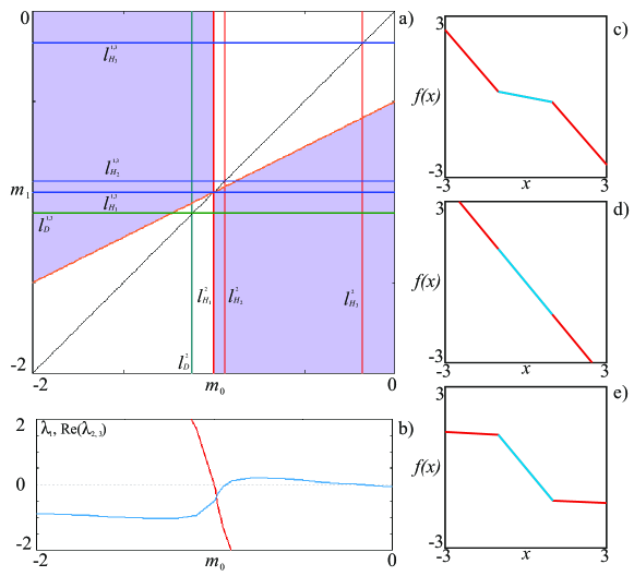
Figure 1: a) Bifurcation lines of equilibrium points on the parameter plane ($m_{0}$, $m_{1}$) for $\alpha=8.4$, $\beta=12$, $\gamma=-0.005$, the red lines correspond to $u_{\rm eq}^{2}$ and the blue lines to $u_{\rm eq}^{1,3}$, the areas of existence of the equilibria $u_{\rm eq}^{1,3}$ are filled by violet color; b) the dependence of the real eigenvalue (red color) and the real part of the complex conjugate eigenvalues (blue color) on the parameter $m_{1}$; c) - e), the examples of the voltage-current characteristics, c) $m_{0}=-0.2$, $m_{1}=-1.15$; d) $m_{0}=-1.2$, $m_{1}=-1.2$; e) $m_{0}=-1.2$, $m_{1}=-0.05$.

Consider the following values of parameters

$$\alpha=8.4,\beta=12,\gamma=-0.005,$$ (7)

which are close to the values, considered in Leonov et al. [2011] and are used for the construction of a hidden attractor. Then for all equilibrium points, one of the eigenvalues, $\lambda_{1}$ is always real and can be positive or negative. Two other eigenvalues $\lambda_{2}$ and $\lambda_{3}$ are complex-conjugated and their real parts can be also positive or negative. Therefore we consider the following types of equilibria:

- $F$

is a stable focus, $\lambda_{1}<0$, $Re(\lambda_{2,3})<0$;

- $SF$-$I$

is a saddle-focus of the first type: there are an unstable one-dimensional manifold and a stable two-dimensional manifold, $\lambda_{1}>0$, $Re(\lambda_{2,3})<0$;

- $SF$-$II$

is a saddle-focus of the second type: there are a stable one-dimensional manifold and an unstable two-dimensional manifold, $\lambda_{1}<0$, $Re(\lambda_{2,3})>0$.

In Fig. 1(a) is shown the plane of parameters $(m_{0},m_{1})$ with the bifurcation curves: blue color denotes the bifurcation curves of the symmetric equilibrium stability, red color denotes the bifurcation curves of the zero equilibrium stability. Areas, filled by violet color, denote the areas of existence of the symmetric equilibria $u_{\rm eq}^{1,3}$. The domains filled by white color correspond to the existence of the only one equilibrium (see conditions (3)). In Fig. 1(b) are shown the plots of $\lambda_{1}$ (red color) and real part of $\lambda_{2,3}$ (blue color) versus the parameter $m_{0}$ for the equilibrium $u_{\rm eq}^{2}$, where one can see the changes of the eigenvalues sign caused by a Hopf bifurcation.

In Fig. 1(a) the following symbols are used for $u_{\rm eq}^{1,3}$ and $u_{\rm eq}^{2}$:

- $l_{H_{1}}^{1,3}$ ($m_{1}\approx-1.0004$), $l_{H_{1}}^{2}$ ($m_{0}\approx-1.0004$)

are the lines of the Hopf bifurcation corresponding to the transition from the saddle-focus of the first type ($SF$-$I$) to the stable focus ($F$);

- $l_{H_{2}}^{1,3}$ ($m_{1}\approx-0.939$), $l_{H_{2}}^{2}$ ($m_{0}\approx-0.939$)

are the lines of the Hopf bifurcation corresponding to the transition from the stable focus ($F$) to the saddle-focus of the second type ($SF$-$II$);

- $l_{H_{3}}^{1,3}$ ($m_{1}\approx-0.1761$), $l_{H_{3}}^{2}$ ($m_{0}\approx-0.1761$)

are the lines of the Hopf bifurcation corresponding to transition from the saddle-focus of the second type ($SF$-$II$) to the stable focus ($F$).

As mentioned above, the parameters $m_{0}$, $m_{1}$ are characterized by the slopes of piecewise linear characteristic. In Fig. 1(c)-(e) are shown examples of voltage-current characteristic for the Chua system (1) for different points of the parameter plane.

2.2 Numerical study of the parameter plane. Bifurcation scenario of the hidden attractors transformations

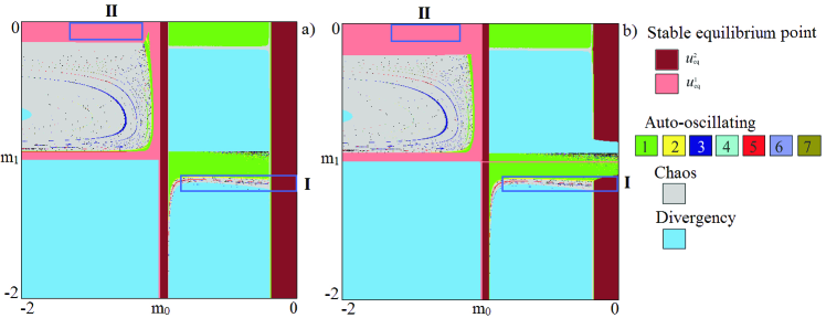
Figure 2: Dynamics of the Chua system, $\alpha=8.4$, $\beta=12$, $\gamma=-0.005$, and initial conditions: a) in the vicinity of the zero equilibrium $u_{\rm eq}^{2}$, $x_{0}=y_{0}=z_{0}=0.0001$; b) in the vicinity of one of the symmetric equilibrium points $u_{\rm eq}^{1}$, $x_{0}=u_{\rm eq}^{x}+0.0001$, $y_{0}=u_{\rm eq}^{y}+0.0001$, $z_{0}=u_{\rm eq}^{z}+0.0001$.

Consider numerically the dynamics and the qualitative behavior of the Chua system (1) in terms of parameters $m_{0}$, $m_{1}$.

In Fig. 2 the charts of dynamical regimes are shown on the parameter plane ($m_{0}$, $m_{1}$). These charts are constructed in the following way. The parameter plane ($m_{0}$, $m_{1}$) is scanned with a small step. The dynamical regime, corresponding to a point on the plane, is determined according to the number of different points in the Poincaré section, defined by $z=0$ after a long enough transition process. Initial conditions are the same for each value of parameters: for the chart in Fig. 2(a) we take initial condition ($x_{0}$, $y_{0}$, $z_{0}$)=(0.0001, 0.0001, 0.0001) in the vicinity of the zero equilibrium $u_{\rm eq}^{2}$. For the chart in Fig. 2(b) we choose initial condition ($x_{0}$, $y_{0}$, $z_{0}$)= ($u_{\rm eq}^{x}$+0.0001, $u_{\rm eq}^{y}$+0.0001, $u_{\rm eq}^{z}$+0.0001) in the vicinity of $u_{\rm eq}^{1}$ (one of the symmetric equilibria, see (4)). Thus, we expect that the dynamical regimes, which are visualized on these charts, are self-excited. On the charts the symmetric stable equilibrium points $u_{\rm eq}^{1,3}$ are marked by pink color, the zero stable equilibrium point $u_{\rm eq}^{2}$ by maroon color, the regime of divergency by blue color, the chaotic dynamics by gray color. The periodic oscillations with different periods are distinguished: the green color for cycles of period-1, the yellow color for cycles of period-2, the dark-blue for cycles of period-3, the blue color for cycles of period-4 and so on (see the color legend in Fig. 2).

We reveal that the complex dynamics of system (1) is developed only in the case that three equilibria coexist. Most of the areas where there is only one equilibrium (see white domains in Fig. 1), belongs to the regime of divergency (see the corresponding domains in Fig. 2). The exceptions are the bands, corresponding to the stable zero equilibrium $u_{\rm eq}^{2}$ for

$$m_{0}>-0.1761\text{\ and\ }m_{1}<\frac{1}{2}(m_{0}-\frac{\beta}{\beta+\gamma}),$$

and the periodic oscillations, associated with the Hopf bifurcation of the zero equilibrium $u_{\rm eq}^{2}$, for

$$m_{1}>-0.1761\text{\ and\ }m_{0}>-\frac{\beta}{\beta+\gamma}.$$

In the case of coexistence of three equilibria the self-excited chaotic attractors are found (gray color). However besides self-excited attractors, here it is possible to find hidden attractors.

In Fig. 2 the blue rectangle (I) is the area of the parameter plane where a hidden chaotic attractor was discovered for the first time Leonov et al. [2011]. For $m_{0}<-0.1761$ (see, the line $l_{H_{3}}^{2}$ of the Hopf bifurcation for the zero equilibrium), all the observed attractors are self-excited. In Fig. 3(a) is shown an example of self-excited Chua attractor from this area of parameters. For $m_{0}>-0.1761$, all dynamical regimes coexist with stable zero equilibrium point. For $m_{0}>-0.1761$, hidden attractors are observed (an example of hidden Chua attractor is in Fig. 3(b), but in some small part of parameter plane a self-excited attractor is found: the phase trajectories, starting from a small neighborhood of the zero equilibrium $u_{\rm eq}^{2}$, tend to the zero stable equilibrium, but the phase trajectories, starting from the vicinity of the symmetric equilibria $u_{\rm eq}^{1,3}$, tend to an attractor (a limit cycle of period-1), in which case the attractors are not hidden. We consider this case in details in Section 3.1.

As mentioned in Section 2.1, the Chua system (1) has symmetry with respect to the parameters $m_{0}$, $m_{1}$. This means that the replacement ($m_{0}$, $m_{1}$) $\to$ ($m_{1}$, $m_{0}$) in the Chua system (1) leads to the replacement of stability of the equilibria: $u_{\rm eq}^{2}$ $\to$ $u_{\rm eq}^{1,3}$. Thus, we can consider another area of possible existence of hidden attractors, which is situated below the line $l_{H_{3}}^{1,3}$ in Fig. 1(a), i.e. before the Hopf bifurcation at the symmetric equilibria. This area is denoted by the blue rectangle (II) in Fig. 2. For $m_{1}>-0.1761$ ($l_{H_{3}}^{1,3}$) there are hidden attractors which cannot be visualized from the initial conditions in a small vicinity of the equilibria.

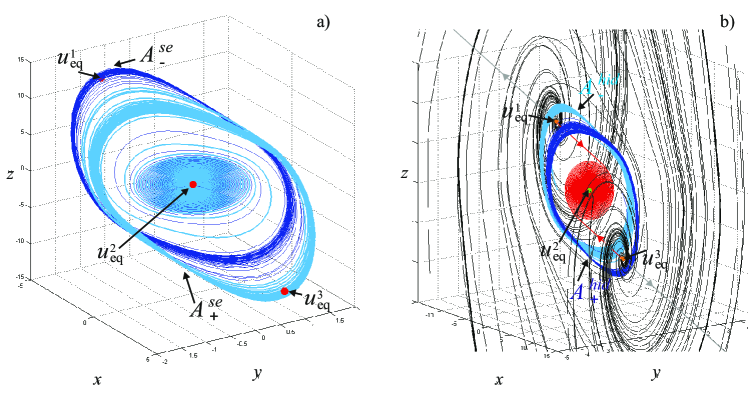
Figure 3: Self-excited and hidden attractors in the Chua system (1) with parameters $\alpha=8.4$, $\beta=12$, $\gamma=-0.005$: a) two symmetric self-excited Chua attractors (cyan and blue domains $A^{se}_{\pm}$) excited from unstable zero equilibrium (parameters $m_{0}=-0.3$, $m_{1}=-1.12$); b) two symmetric hidden chaotic Chua attractors (cyan and blue domains $A^{hid}_{\pm}$). Red and gray trajectories from unstable manifold of the symmetric saddle-focuses equilibria $u_{\rm{eq}}^{1,3}$ (orange dots) are attracted to locally stable equilibrium $u_{\rm{eq}}^{2}$ (green dot) and infinity, respectively. Black trajectories are stable manifolds of $u_{\rm{eq}}^{1,3}$ (parameters $m_{0}=-0.121$, $m_{1}=-1.143$).

3 Hidden twin attractors

3.1 Merged twin attractors

Now we consider the dynamics of the Chua system (1) with the parameters corresponding to the rectangle (I) in Fig. 2, the zoom of which is shown in Fig. 4(a). For this area, for each point of parameter plane the initial conditions are the same as in the vicinity of equilibrium $u_{\rm eq}^{1}$. In Fig. 4(b) the same fragment of the chart is constructed by the so-called continuation method for choosing initial conditions, i.e., for each new value of parameter as initial point, the same value is chosen as the final point (obtained from the previous value of the parameter). We use this method to identify the area where hidden attractors exist. In Fig. 4(b) we mark a point in which we start our calculations, and the arrows show the direction of scanning.

The analysis of stability of the equilibrium points in this area (see Fig. 1(a)) shows that for $m_{0}=0$ three equilibrium points exist: two symmetric saddle-focus $SF$-$I$ and one stable focus $F$ (zero equilibrium). In Fig. 4(a) and (b) is shown the bifurcation line of the loss of stability of the zero equilibrium for $m_{0}\approx-0.1761$ ($l_{H_{3}}^{2}$). In the area colored in the maroon, the zero equilibrium point is characterized by one negative real number and two complex conjugate numbers with negative real part; after crossing the bifurcation line ($l_{H_{3}}^{2}$) the real parts of the conjugate-complex eigenvalues become positive, and a stable focus is transformed into a saddle-focus with a two-dimensional unstable manifold. For the same parameters there exist also two symmetric equilibria, which are characterized by one positive real number and two complex-conjugate eigenvalues with a negative real part.

In the chart of dynamical regimes in Figs. 4(a) and (b), for fixed parameter $m_{0}$ and decreasing parameter $m_{1}$, one can observe a transition from a limit cycle of period-1 to a chaotic attractor. This transition corresponds to the Feigenbaum scenario (the cascade of period-doubling bifurcations) and it occurs in both the self-excited and the hidden attractors.

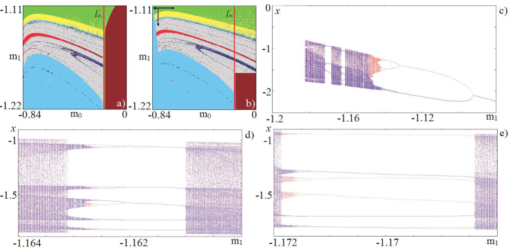
Figure 4: a), b) magnified fragment (I) of the chart of dynamical regimes for different initial conditions, $\alpha=8.4$, $\beta=12$, $\gamma=-0.005$; c) bifurcation diagram: red and violet colors correspond to different initial conditions, $m_{0}=-0.121$; d), e) magnified fragments of bifurcation diagram.

To analyze the birth of bifurcations, we construct a bifurcation diagram versus parameter $m_{1}$. In Fig. 4 are shown bifurcation diagram (c) and its magnified fragments (d, e). In Figs. 4(c)-(e) is shown the dependence of the variable $x$, in the Poincaré section by the plane $z=0$ (for $m_{0}=-0.1210$), on the parameter $m_{1}$. In the diagram in Fig. 4(c), we identify the value of the parameter $m_{1}^{*}\approx-1.1247$ corresponding to the transition from a self-excited attractor to a hidden attractor. For $-1.0929<m_{1}<-1.0800$ the system exhibits one limit cycle with period-1 in Fig. 4(c). For $m_{1}\approx-1.0929$, the limit cycle is split into two different period-1 limit cycles via a pitchfork bifurcation. The pitchfork bifurcation is typical in the Chua system since this system exhibits an inner symmetry. For $-1.1317<m_{1}<-1.0929$ two limit cycles of period-1 coexist, these cycles are symmetric to each other. Notice that for $m_{1}\approx-1.1247$ these two period-1 limit cycles become hidden. For $m_{1}\approx-1.1317$ both limit cycles become limit cycles of period-2 via a period doubling bifurcation. By continuous decreasing the parameter $m_{1}$, after the sequence of period-doubling bifurcations, as shown in Fig. 4(c), the two limit cycles are transformed into two different hidden chaotic attractors, respectively. In this case these attractors coexist with a symmetric twin-attractor, and a stable zero equilibrium point. For $m_{1}\approx-1.1483$ the twin-attractors are merged into one, which by further decreasing the parameter $m_{1}$, forms an increasingly larger chaotic set. For $m_{1}\approx-1.1609$, a periodic window of period-5 emerges (in Fig. 4(d) is shown a magnified fragment near the periodic window of period-5). The same scenario takes place for the period-5 cycle. For $m_{1}\approx-1.1621$ the period-5 limit cycle is split into two symmetric period-5 limit cycles via a pitchfork bifurcation. For $-1.1626<m_{1}<-1.1621$ two limit cycles of period-5 coexist. For $m_{1}\approx-1.1621$ both limit cycles bifurcate into two limit cycles of period-10 via a period-doubling bifurcation. Upon further decreasing the parameter $m_{1}$, after a sequence of period-doubling bifurcations, two hidden chaotic attractors emerge. Then they merged at $m_{1}\approx-1.1628$, and collapse with the chaotic set of the previous attractor at $m_{1}\approx-1.1631$.

Upon a further decrease of the parameter $m_{1}$, a periodic window of period-3 emerges (Fig. 4(e) shows a magnified fragment near a period-3 window). In this case there is no pitchfork bifurcation, and for $-1.1714<m_{1}<-1.1684$ two symmetric hidden cycles of period-3 coexist. For $m_{1}\approx-1.1714$ both period-3 cycles become a pair period-6 limit cycles via a period doubling bifurcation. Further decrease of the parameter $m_{1}$ gives rise to a cascades of period-doubling bifurcations. In this case we can not see the merging of two chaotic attractors, but for $m_{1}\approx-1.1719$ two hidden symmetric attractors merge into a chaotic set.

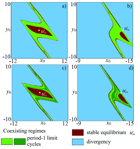
Figure 5: Basins of attraction of coexisting self-excited attractors of the Chua system with $\alpha=8.4$, $\beta=12$, $\gamma=-0.005$, $m_{0}=-0.121$: a) limit cycle of period-1 before pitchfork bifurcation $m_{1}=-1.09$, in the section defined by the plane $z_{0}=0.00001$; b) in the section defined by the plane $z_{0}=u_{\rm eq}^{z}$; c) period-1 limit cycles after pitchfork bifurcation at $m_{1}=-1.1$, in the section defined by the plane $z_{0}=0.00001$; d) in the section defined by the plane $z_{0}=u_{\rm eq}^{z}$.

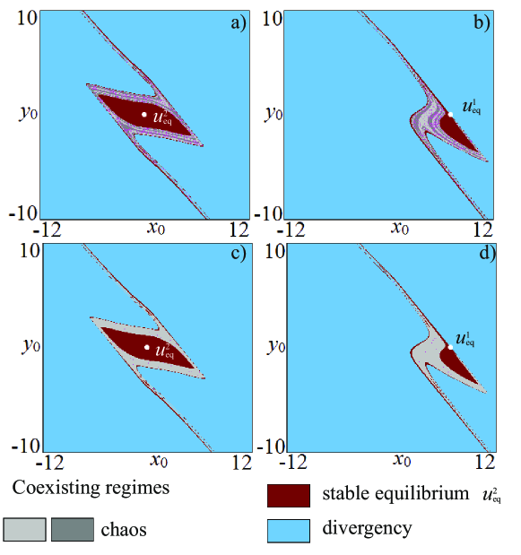
Figure 6: Basins of attraction of coexisting hidden attractors of the Chua system with $\alpha=8.4$, $\beta=12$, $\gamma=-0.005$, $m_{0}=-0.121$: a) twin hidden chaotic attractors for $m_{1}=-1.143$, in the section defined by the plane $z_{0}=0.0001$; b) in the section defined by the plane $z_{0}=u_{\rm eq}^{z}$; c) merged hidden chaotic attractors for $m_{1}=-1.15$, in the section defined by the plane $z_{0}=0.0001$; d) in the section defined by the plane $z_{0}=u_{\rm eq}^{z}$.

To analyze localization of hidden attractors in the phase space, and transition from self-excited to hidden attractors, we consider the basins of attraction under varying parameter. Firstly, we consider the case that a self-excited attractor is realized: $m_{0}=-0.121$, $m_{1}=-1.09$. Since its basin of attraction in three-dimensional phase space is difficult to analyze, we analyze two-dimensional sections of this volume at various planes, which correspond to two-dimensional planes of initial conditions. To distinguish between hidden and self-excited attractors, the dynamical behavior of the model in the vicinity of equilibria is crucial. That is why we consider two sections of phase volume: in the vicinity of the zero equilibrium $u_{\rm eq}^{2}$ and in the vicinity of one of the symmetric equilibria $u_{\rm eq}^{1}$ (for the other symmetric equilibrium $u_{\rm eq}^{3}$, the structure of the basin is similar).

In Fig. 5 is shown the two-dimensional plane of initial conditions for vicinities of equilibria points and for different values of parameter $m_{1}$. The regime of divergency is marked by blue color, the area of attraction of the stable zero equilibrium is marked by maroon color. The areas of attraction regimes of different period-1 limit cycles are denoted by two different green colors. The location of the equilibrium points in the plane is identified by white dots. In Fig. 5(a) is shown a two-dimensional plane of initial conditions for fixed $z_{0}=0.0001$ in the vicinity of the zero equilibrium $u_{\rm eq}^{2}$ (stable focus $F$). For $m_{1}=-1.09$ in system (1) the coexistence of a period-1 limit cycle, before the pitchfork bifurcation, and the stable zero equilibrium is observed. In Fig. 5(a) is shown the structure of the basins of attraction of two coexisting regimes. There is a rather large basin of attraction surrounding the stable zero equilibrium (maroon color), and a large area of divergency. Between these two areas we have an area of stable periodic oscillations, which represents the basin of attraction of a period-1 limit cycle. The boundary between the areas of divergency and self-excited limit cycle is indicated by a thick line, which corresponds to the stable zero equilibrium. In Fig. 5(b) is shown a vicinity of one of the symmetric points $z_{0}=u_{\rm eq}^{z}$ (saddle-focuses SF-I). The symmetric equilibrium state is located on the boundary between the basin of attraction of the stable limit cycle and the area of divergency. In this case we cannot affirm that the limit cycle is a hidden attractor because if we start to iterate a trajectory, with a randomly chosen initial state in the vicinity of symmetric equilibrium points, it can either diverge from the initial state, or tend to the limit cycle.

After the pitchfork bifurcation ($m_{0}=-1.1$) two symmetric limit cycles occur. In Figs. 5(c),(d) are shown two planes of initial conditions with basins of attraction of symmetric limit cycles in the vicinity of the two equilibria for fixed third initial conditions $z_{0}=0.00001$ and $z_{0}=u_{\rm eq}^{z}$, in which case, the two different green colors correspond to the basins of attraction of the two symmetric limit cycles ($m_{1}=-1.1$). In this case after the pitchfork bifurcation, the basin of attraction of original limit cycle is split into two basins of attraction of the two symmetric period-1 limit cycles. These basins have a complex but symmetric structure. In this case the equilibrium $u_{\rm eq}^{1}$ is also situated on the boundary of the basins of attraction of the two limit cycles, implying that the limit cycles are self-excited for $m_{1}>m_{1}^{*}$.

Next, we decrease parameter $m_{1}$ such that it becomes less then $m_{1}^{*}$. In this case the attractors become hidden, while bifurcating into chaotic dynamics, and we observe the corresponding changes in the structure in the plane of initial conditions. In Fig. 4 is shown that hidden twin chaotic attractors exist, for instance, at $m_{1}\approx-1.141$, and with decreasing parameter $m_{1}$ these two attractors merged (for $m_{1}\approx-1.147$). In Fig. 6 are shown the planes of initial conditions for the twin chaotic attractors (a) and (b), and the merged chaotic attractor (c) and (d). In Figs. 6(a),(b) the basins of attraction of the two different chaotic attractors are identified by different shaded gray colors. The composition of the basins in the plane of initial states near the vicinity of the zero equilibrium point is the same as in the case of self-excited limit cycle. We observe the basins of attraction of the twin chaotic attractors and the basin of attraction of zero stable equilibrium point in the center. But the structure of the plane of initial states in the section near the vicinity of the symmetric equilibrium points has a significant distinction. The basin of attraction of the stable zero equilibrium $u_{\rm eq}^{2}$ at the center is combined with the another part of the basin of attraction of the stable zero equilibrium point $u_{\rm eq}^{2}$ on the boundary of the area of divergency, and a saddle equilibrium $u_{\rm eq}^{1}$ is located on the boundary between the basin of attraction of the stable zero equilibrium point and the area of divergency. Consequently, a twin chaotic attractor becomes hidden because if we choose initial states near one of the equilibrium points, then we cannot reach the chaotic attractors.

In Figs. 6(c) and d are shown the same illustrations for merged hidden chaotic attractor. In this case one can see that the basin of attraction of the merged hidden attractor represents the combining of the areas of attraction of each twin-hidden attractors. In the vicinity of the saddle equilibrium we also see only two possible regimes: the stable zero equilibrium and the divergency. It follows that the merged attractor is the hidden one.

3.2 Separated twin-attractors

Now we consider the dynamics of the Chua system (1) and the features of hidden attractors in another area of the parameter plane, which is marked by the blue rectangles (II) in Fig. 2. In Fig. 7(a) is shown the zoom of fragment (II). For the continuation method of changing initial conditions, the starting point is denoted on the parameter plane, and we scan the plane of parameters in different directions in accordance with the arrows in this figure.

The analysis of stability of equilibria (Fig. 1(a)) shows that in this area there are two symmetric stable focuses ($F_{1}$, $F_{2}$) and one saddle-focus of the first type (SF-I) at the zero equilibrium point.

By numerical integration the trajectories starting from the vicinity of any equilibrium point in rectangle (II) can reach only one of the symmetric equilibrium points (Fig. 2). But we can see in Fig. 7(a) that for some special initial conditions it is possible to observe hidden attractors. In particular, the bifurcation scenario associated with the hidden attractors from the area of the parameter plane (II) is the same as that in the area (I): one can observe chaotic dynamics resulting from of a cascade of period-doubling bifurcations.

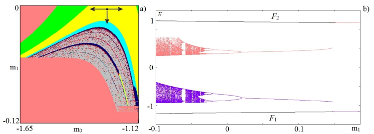
Figure 7: a) the magnified fragment (II) of the chart of dynamical regimes for continuation method of changing initial conditions, $\alpha=8.4$, $\beta=12$, $\gamma=-0.005$; b) bifurcations diagram: black, red, and violet colors correspond to different initial conditions, $m_{0}=-1.2$.

To analyze the bifurcations and transformations in this case, let us consider a bifurcation diagram. In Fig. 7(b) are shown diagrams for different initial conditions for $m_{0}=-1.2$, as a function of the parameter $m_{1}$ in the Poincaré section by the plane $z=0$. The black lines correspond to initial condition near the symmetric equilibrium points (the scanning of parameter $m_{1}$ was realized by the continuation method to choose initial conditions), and these lines mark the coexisting stable focuses ($F_{1}$ and $F_{2}$). For the red and violet bifurcation diagrams the initial conditions are chosen in the following way: $x_{0}=\mp 1.2$, $y_{0}=\mp 0.0005$, $z_{0}=0$, respectively. For these initial conditions for $m_{1}=0$ we have two symmetric period-2 limit cycles, and from these points we scan the parameter intervals $m_{1}$ $[-0.2,0.1]$ in two directions (to the right and to the left).

Figure 8: Example of two symmetric hidden chaotic Chua attractors (blue and cyan domains $\mathcal{A}^{\rm hid}_{\pm}$), $m_{1}=-0.05$. Red trajectories from unstable manifold ${\rm M_{0}^{\rm unst}}$ of the zero saddle-focus equilibrium $u_{\rm{eq}}^{2}$ (orange dot) are attracted to locally stable equilibria $u_{\rm{eq}}^{1,3}$ (green dots); gray trajectories are stable manifold ${\rm M_{0}^{\rm st}}$ of $u_{\rm{eq}}^{2}$; green trajectories are stable manifolds ${\rm M_{\pm}^{\rm st}}$ of $u_{\rm{eq}}^{1,3}$.

For $m_{1}=0.2$ there are two symmetric stable equilibrium points. If the parameter $m_{1}$ decreases, then at $m_{1}\approx 0.15$ a limit cycle emerges near each symmetric equilibrium point. In the bifurcation diagram one can see the hard birth of the cycles, because of the form of nonlinearity (piecewise-linear characteristic of the Chua circuit). As $m_{1}$ decreases, we see stable focuses and two coexisting limit cycles, undergoing a period-doubling bifurcation and transition to chaos. However, for this area of parameter plane there is no a pitchfork bifurcation of limit cycles and a merging of chaotic attractors. In this case two bifurcation diagrams in Fig. 7 (b) do not cross each other and are separated by the saddle point at the zero equilibrium. In Fig. 8 the example of two symmetric hidden chaotic Chua attractors are shown for $m_{1}=-0.05$. By red, gray and green colors in Fig. 8 are shown the stable and unstable manifolds in the vicinity of equilibrium points. Gray and green trajectories were constructed by integration in inverse time for initial conditions in the vicinity of equilibrium points (gray lines are near saddle-focus, green lines are near stable focuses). Red trajectories tend to the symmetric equilibria and are obtained by the integration in forward time near the zero equilibrium.

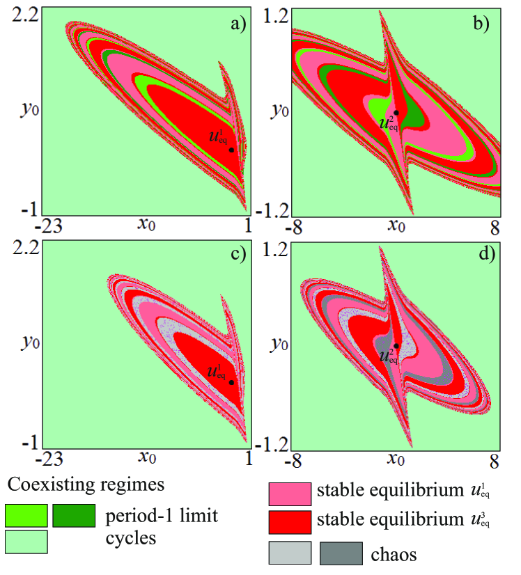
Figure 9: Basins of attraction of coexisting attractors of the Chua system (1) $\alpha=8.4$, $\beta=12$, $\gamma=-0.005$, $m_{0}=-1.2$: a) twin hidden period-1 attractors with $m_{1}=0.1$, and cross-section by the plane $z_{0}=u_{\rm eq}^{z}$; b) cross-section by the plane $z_{0}=0.0001$; c) twin hidden chaotic attractors with $m_{1}=-0.05$, cross-section by the plane $z_{0}=u_{\rm eq}^{z}$; d) cross-section by the plane $z_{0}=0.0001$.

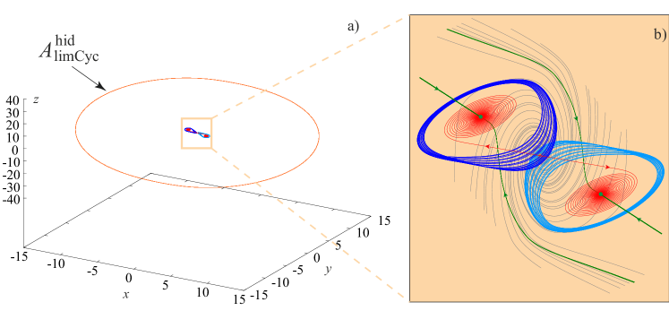
Figure 10: Multistability with 5 coexisting attractors in the Chua system (1) with $\alpha=8.4$, $\beta=12$, $\gamma=-0.005$, $m_{0}=-1.2$, $m_{1}=-0.05$. Coexistence of hidden periodic attractor (orange trajectory $\mathcal{A}^{\rm hid}_{\rm limCyc}$ is a stable limit cycle) and two symmetric hidden chaotic Chua attractors (blue and cyan domains). Here the basins of attraction of the periodic and the two symmetric Chua attractors do not intersect with a small neighborhood of the equilibria, thus, the attractors are hidden.

To analyze the structure of the phase space and the localization of hidden attractors in the phase space, we consider two-dimensional planes of initial conditions. Then we can study the basins of attraction of co-existing attractors. As in the previous case we consider two-dimensional sections of the three-dimensional phase space of initial states in the vicinity of one of the stable symmetric equilibria $u_{\rm eq}^{1}$, and in the vicinity of the zero equilibrium $u_{\rm eq}^{2}$. In Fig. 9 is shown the structure of areas of attraction for different parameters of $m_{1}$ and $m_{0}=-1.2$, and for different cross-section of the phase space. In Fig. 9(a) and (b) are shown the basins of attraction of coexisting attractors for $m_{1}=0.1$ in the vicinity of one stable focus $F_{1}$ (a) and in the vicinity of the zero saddle equilibrium (b), the location of equilibrium points are marked in the plane by black dots. In this case in the bifurcation diagram one can see two coexisting symmetric equilibrium points and two symmetric cycles of period-1. Also it is observed a new period-1 limit cycle, surrounding all regimes described above, and the dynamics near the equilibria is developed inside this limit cycle of sufficiently large radius. So, for this area of parameters we have five coexisting attractors. We shaded the areas of attraction of different symmetric period-1 limit cycles by green color. The area of attraction of the outside limit cycle is marked on the plane by light green color. We use the pink and red colors to denote the basins of attraction of the two symmetric equilibria $u_{\rm eq}^{1}$ and $u_{\rm eq}^{3}$, respectively.

Firstly, we consider a vicinity of the stable equilibrium (Fig. 9(a)). In the vicinity of the stable equilibrium one can see a basin of attraction of one of the symmetric stable equilibrium points. Also, there are the basin of attraction of another symmetric stable equilibrium point, and the symmetric basins of attraction of two symmetric limit cycles. The complex structure of their basins is represented by the area of attractions in the form of bands, which are spiralled together, and their boundaries have self-similar patterns, i.e., fractal structures. Also, there is a basin of attraction of the external limit cycle, which surround all other basins of attraction.

Then we consider a plane of initial conditions and the basins of attraction of different attractors in the vicinity of the saddle equilibrium point (Fig. 9(b)). We can see that the phase trajectories, starting from the vicinity of the saddle point, can reach one of the stable symmetric equilibria only. The zero equilibrium point $u_{eq}^{2}$ is located on a boundary between the attracting areas of different symmetric stable equilibria. The areas of attraction are symmetric to each other, and a boundary between these areas represents the stable manifold of the zero saddle-focus. Consequently, if we choose initial conditions in the vicinity of any equilibrium point, we will reach one of the stable equilibrium points and, thus, all of the limit cycles are hidden attractors.

Let us decrease the parameter $m_{1}$ so that chaotic dynamics emerges, and consider the basins of attraction of the coexisting stable symmetric equilibria, the chaotic attractors, and the external limit cycle. In Fig. 9(c) and (d) are shown two planes of initial conditions in the vicinity of the equilibrium points for $m_{1}=-0.05$. By two shades of gray color we identify the basins of attraction of the coexisting twin-chaotic attractors. It is rather easy to distinguish the basins of attraction for these chaotic attractors because the attractors in the phase space are separated by the zero saddle equilibrium. For decreasing parameter $m_{1}$ the structure of the basin of attraction persists. In place of the areas of two symmetric period-1 limit cycles one sees the basins of attraction of the symmetric chaotic attractors. In this case the order of alternation of the basin of attraction of different attractors remains the same. The structure of the basin of attraction in the vicinity of the saddle equilibrium point persists: the saddle point is located on the boundary of the basins of attraction of two symmetric equilibrium points, and the boundary corresponds to an stable manifold of the saddle point.

In Fig. 10 (a),(b) is shown a structure of the phase space in the above case, where we see a coexisting large stable limit cycle (orange color in Fig. 10 (a)) and two separated hidden chaotic Chua attractors (blue and cyan domains Fig. 10  (b)) from Fig. 8. The basins of attraction of periodic and chaotic attractors do not intersect with a small neighborhood of the equilibria, thus, the attractors are hidden. Therefore in this case there are 5 coexisting attractors: two stable equilibria, one hidden limit cycle, and two hidden “twin” attractors.

Thus, we reveal two area on the parameter plane ($m_{0}$, $m_{1}$), where we observe hidden attractors. Observe that for the physical realization of the Chua circuit and observation of hidden attractors we need nonnegative parameters $\alpha$, $\beta$, $\gamma$. For example, both configurations of hidden attractors cited above are observed for the case $\gamma=0$ in Rocha & Medrano-T [2015, 2016]; and for the positive $\gamma$ one may consider, for example, the following two sets of parameters: $\alpha=8.4562,\beta=12.0732,\gamma=0.0052,m_{0}=-0.1768,m_{1}=-1.1468$ and $\alpha=8.4,\beta=12,\gamma=0.005,m_{0}=-0.12,m_{1}=-1.143$.

Note that the existence of hidden attractors in the Chua system can be effectively predicted by the describing function method (DFM) Leonov et al. [2011]; Rocha & Medrano-T [2015]; Kuznetsov et al. [2017a]. The classical DFM (see, e.g. Krylov & Bogolyubov [1947]; Khalil [2002]) is only an approximate method which gives the information on the frequency and amplitude of periodic orbits. However DFM may lead to wrong conclusions about the existence of periodic orbits and does not provide initial data for the localization of periodic orbits. But for the systems of special type with a small parameter, DFM can be rigorously justified. For this purpose, following references Leonov et al. [2011]; Leonov & Kuznetsov [2013], we introduce a coefficient $k$ and represent the linear part and nonlinearity in (2) as follows:

$${P_{0}}={P}+k{qr}^{*}=\left(\begin{array}[]{ccc}-\alpha(m_{1}+1+k)&\alpha&0\\ 1&-1&1\\ 0&-\beta&-\gamma\\ \end{array}\right),$$ (8)

$$\psi(\sigma)=\phi(\sigma)-k\sigma=(m_{0}-m_{1})\,{\rm sat}(\sigma)-k\sigma,$$

where $\lambda^{{P}_{0}}_{1,2}=\pm i\omega_{0}$, $\lambda^{{P}_{0}}_{3}=-d<0$. Then we consider a small parameter $\varepsilon$, change $\psi(\cdot)$ by $\varepsilon\psi(\cdot)$, and reduce by a non-singular linear transformation ${w}={Su}$ system (8) to the following form

$$\dot{w}={A}{w}+{b}\varepsilon\psi({u}^{*}{y}),$$ (9)

$${A}=\left(\begin{array}[]{ccc}0&-\omega_{0}&0\\ \omega_{0}&0&0\\ 0&0&-d\\ \end{array}\right),\ {b}=\left(\begin{array}[]{c}b_{1}\\ b_{2}\\ b_{3}\\ \end{array}\right),\ {c}=\left(\begin{array}[]{c}1\\ 0\\ -h\\ \end{array}\right).$$

Theorem Leonov et al. [2011]; Leonov & Kuznetsov [2013]; Kuznetsov et al. [2017a] Consider the describing function $\Phi(a)=\int_{0}^{2\pi\!/\omega_{0}}\psi(a\,\cos(\omega_{0}t))\cos(\omega_{0}t)dt.$ If there exists a positive $a_{0}$ such that $\Phi(a_{0})=0,\quad b_{1}\Phi^{\prime}(a_{0})<0,$ then system (9) has a stable periodic solution with the initial data $w_{0}=\big{(}a_{0}+O(\varepsilon),0,O(\varepsilon)\big{)}$ and period $T=\frac{2\pi}{\omega_{0}}+O(\varepsilon)$.

This theorem gives an initial point for the numerical computation of periodic solution (starting attractor) in the system with small parameter. Then, using the method of numerical continuation and gradually increasing $\varepsilon$, one can numerically follow the transformation of the starting attractor.

It turns out that for the numerical localization of the considered hidden attractors we can skip the multistep procedure based on numerical continuation and use the initial data $u_{0}=S^{-1}w_{0}$ for the localization of hidden attractors in the initial system (). For the parameters $\alpha=8.4,\beta=12,\gamma=-0.005,m_{0}=-1.2,m_{1}=-0.05$ we get: a) $k=-0.8890,\omega_{0}=2.0260,a_{0}=1.5187$ and the corresponding initial data $\pm(1.5187,0.0926,-2.1682)$ allows us to visualize two symmetric hidden chaotic attractors; b) $k=-0.1244,\omega_{0}=3.2396,a_{0}=11.7546$ and the corresponding initial data $(11.7546,9.7044,-16.7367)$ allows us to localize the hidden periodic attractor (see Fig. 10). For the parameters $\alpha=8.4,\beta=12,\gamma=-0.005,m_{0}=-0.121,m_{1}=-1.143$ we get $k=0.2040,\omega_{0}=2.0260,a_{0}=6.3526$ and the corresponding initial data $\pm(6.3526,0.3874,-9.0694)$ allows us to visualize two symmetric hidden chaotic attractors (see Fig. 3(b)).

4 Scenario of the birth of hidden attractors

In Sections 3.1 and 3.2 we have shown the opportunity of existence of hidden attractors in different areas of the parameter plane. In order to study the scenario of the emergence of hidden attractors we use numerical bifurcation analysis by the software package XPP AUTO Ermentrout [2002].

4.1 Formation of separated hidden attractors

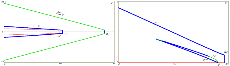
Figure 11: Bifurcation diagram of the Chua system (1), $\alpha=8.4$, $\beta=12$, $\gamma=-0.005$, $m_{1}=-0.05$.

Firstly we consider hidden attractors from the area (II) in the parameter plane ($m_{0}$, $m_{1}$) (Fig. 2). In Fig. 11(a) is shown the bifurcation diagram of the Chua system (1) for parameters (7) and $m_{1}=-0.05$. In the diagram red and black color denote stable and unstable equilibrium points, green and blue colors denote stable and unstable limit cycles, respectively. At $m_{0}\approx-0.1761$ the Hopf bifurcation ($H_{3}^{2}$) takes place, that is in a good agreement with the results obtained by linear analysis in Section 2.1 and by numerical simulations in Section 3.2. In this case the supercritical Hopf bifurcation occurs: the zero equilibrium point loses stability and a limit cycle $A_{limCyc}^{hid}$ is born. With decreasing of parameter $m_{0}$ the radius of limit cycle is increased. At $m_{0}\approx-0.939$ a second Hopf bifurcation ($H_{2}^{2}$) emerges, where the zero equilibrium becomes stable, which is accompanied by the hard birth of an unstable limit cycle $C_{1}$. The radius of the internal unstable cycle $C_{1}$ surrounding the zero equilibrium increases initially according to square root of 2, upon a further decrease of the parameter $m_{0}$. At $m_{0}\approx-1.0004$ occurs a third Hopf bifurcation ($H_{1}^{2}$), which is a pitchfork bifurcation of the zero equilibrium, in which case two stable symmetric equilibria are born, and the zero equilibrium become unstable. In this case the limit cycle $C_{1}$ surrounds all equilibria, splits the limit cycle $A_{limCyc}^{hid}$ and equilibria in the phase space, and forms the boundary of the basin of attraction of the limit cycle $A_{limCyc}^{hid}$. The pitchfork bifurcation ($H_{1}^{2}$) is accompanied by the occurrence of two symmetric pairs of limit cycles $C_{2}^{st}$ and $C_{2}^{unst}$, which are denoted in the magnified fragment of the diagram in Fig. 11(b). The birth of the limit cycles is a result of a saddle-node bifurcation, i.e. a pair of limit cycles (stable and unstable) are born, along with its identical symmetric pair. Thus, the stable limit cycle $C_{2}^{st}$ is surrounded by the unstable limit cycle $C_{1}$ on the one side, and by the unstable limit cycle $C_{2}^{unst}$ on the other side, making it unreachable from the vicinity of stable equilibria points and also from the vicinity of unstable equilibrium points. Thus, the limit cycles $C_{2}^{st}$, and the chaotic attractor, which occur on the base of this limit cycle are hidden.

4.2 Formation of merged hidden attractors

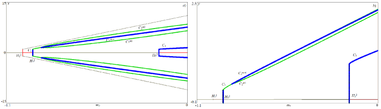
Figure 12: Bifurcation diagram for the Chua system (1) with $\alpha=8.4$, $\beta=12$, $\gamma=-0.005$, $m_{1}=-1.11$.

Formation of hidden attractors in the area (I) in the parameter plane ($m_{0}$, $m_{1}$) is as follows. In Fig. 12 the corresponding bifurcation diagrams are shown. In this case it is better to exam the bifurcation diagrams by increasing the parameter $m_{0}$. At $m_{0}\approx-1.0004$ the Hopf bifurcation ($H_{1}^{2}$) occurs, where the unstable zero equilibrium point becomes stable, simultaneously with pitchfork bifurcation, and as a result of which two unstable equilibria are born. At $m_{0}\approx-0.939$ the zero equilibrium point undergoes a supercritical Hopf bifurcation ($H_{2}^{2}$), and as a result the zero equilibrium point loses stability and a stable limit cycle $C_{1}$ is born, where it is situated between two symmetric unstable equilibria in projections onto the $x$ and $z$ variables, where it surrounds all equilibria in a projection of $y$-variable. Upon increasing the parameter $m_{0}$, the limit cycle undergoes a symmetry breaking bifurcation (it is the same as a pitchfork bifurcation), and splits into two stable symmetric limit cycles $C_{2}^{st1}$, $C_{2}^{st2}$ and one unstable limit cycle $C_{2}^{unst}$. At $m_{0}\approx-0.1761$ ($H_{3}^{2}$) the zero equilibrium point changes stability again. In this case the bifurcation is subcritical, and as a result the unstable limit cycle $C_{3}$ is born. The limit cycle $C_{3}$ forms boundaries of the basin of attraction of the zero stable equilibrium point. In Fig. 12(b) is shown the projection of the $y$-variable. Thus, for $m_{0}>-0.1761$ ($H_{3}^{2}$) the limit cycles $C_{2}^{st1}$ and $C_{2}^{st2}$ are isolated from all equilibria by the unstable limit cycle $C_{3}$, and these symmetric limit cycles $C_{2}^{st1}$ and $C_{2}^{st2}$ and chaotic attractors, which occur on the base of these cycles for another set of parameters, are hidden.

5 Conclusion

The dynamics of the Chua circuit gives a complex picture in the space of controlling parameters. The areas with similar behavior exist, and the detailed study of the dynamics of the Chua system in these areas allows one to reveal new hidden attractors. It is shown that the formation of hidden attractors is connected with the subcritical Hopf bifurcations of equilibrium points and the saddle-node bifurcations of the limit cycles. In general, the conjecture is that for a globally bounded autonomous system of ODE with asymptotically stable equilibrium point, the subcritical Hopf bifurcation leads to the birth of a hidden attractor. In two different areas of parameter plane it was found two types of hidden attractors, namely, merged and separated attractors. These features of hidden attractors are connected with the location of stable and unstable equilibria and with the associated with them unstable limit cycles in the phase space. The open questions are what is the maximum number of coexisting attractors that can be exhibited in the Chua system (1) and how many of the coexisting attractors can be hidden.

Acknowledgments This work was supported by the Russian Science Foundation project 14-21-00041 (sections 2.2-4). L.Chua’s research is supported by grant no. AFOSR FA 9550-13-1-0136.

References

- Aizerman [1949] Aizerman, M. A. [1949] “On a problem concerning the stability in the large of dynamical systems,” Uspekhi Mat. Nauk (in Russian) 4, 187–188.
- Alli-Oke et al. [2012] Alli-Oke, R., Carrasco, J., Heath, W. & Lanzon, A. [2012] “A robust Kalman conjecture for first-order plants,” IFAC Proceedings Volumes (IFAC-PapersOnline) 7, 27–32,
- Bao et al. [2015a] Bao, B., Hu, F., Chen, M., Xu, Q. & Yu, Y. [2015a] “Self-excited and hidden attractors found simultaneously in a modified Chua’s circuit,” International Journal of Bifurcation and Chaos 25, art. num. 1550075.
- Bao et al. [2015b] Bao, B., Jiang, P., Wu, H. & Hu, F. [2015b] “Complex transient dynamics in periodically forced memristive Chua’s circuit,” Nonlinear Dynamics 79, 2333–2343.
- Bao et al. [2016] Bao, B. C., Li, Q. D., Wang, N. & Xu, Q. [2016] “Multistability in Chua’s circuit with two stable node-foci,” Chaos: An Interdisciplinary Journal of Nonlinear Science 26, art. num. 043111.
- Barabanov [1988] Barabanov, N. E. [1988] “On the Kalman problem,” Sib. Math. J. 29, 333–341.
- Bautin [1939] Bautin, N. N. [1939] “On the number of limit cycles generated on varying the coefficients from a focus or centre type equilibrium state,” Doklady Akademii Nauk SSSR (in Russian) 24, 668–671.
- Belykh & Chua [1993] Belykh, V. & Chua, L. [1993] “A new type of strange attractor related to the Chua’s circuit,” J. Circuits Syst. Comput. 3, 361–374.
- Bernat & Llibre [1996] Bernat, J. & Llibre, J. [1996] “Counterexample to Kalman and Markus-Yamabe conjectures in dimension larger than 3,” Dynamics of Continuous, Discrete and Impulsive Systems 2, 337–379.
- Bilotta & Pantano [2008] Bilotta, E. & Pantano, P. [2008] A gallery of Chua attractors, Vol. Series A. 61 (World Scientific).
- Borah & Roy [2017] Borah, M. & Roy, B. K. [2017] “Hidden attractor dynamics of a novel non-equilibrium fractional-order chaotic system and its synchronisation control,” 2017 Indian Control Conference (ICC), pp. 450–455.
- Bragin et al. [2011] Bragin, V., Vagaitsev, V., Kuznetsov, N. & Leonov, G. [2011] “Algorithms for finding hidden oscillations in nonlinear systems. The Aizerman and Kalman conjectures and Chua’s circuits,” Journal of Computer and Systems Sciences International 50, 511–543.
- Brzeski et al. [2017] Brzeski, P., Wojewoda, J., Kapitaniak, T., Kurths, J. & Perlikowski, P. [2017] “Sample-based approach can outperform the classical dynamical analysis - experimental confirmation of the basin stability method,” Scientific Reports 7, art. num. 6121.
- Burkin & Khien [2014] Burkin, I. & Khien, N. [2014] “Analytical-numerical methods of finding hidden oscillations in multidimensional dynamical systems,” Differential Equations 50, 1695–1717.
- Chaudhuri & Prasad [2014] Chaudhuri, U. & Prasad, A. [2014] “Complicated basins and the phenomenon of amplitude death in coupled hidden attractors,” Physics Letters A 378, 713–718.
- Chen [2015] Chen, G. [2015] “Chaotic systems with any number of equilibria and their hidden attractors,” 4th IFAC Conference on Analysis and Control of Chaotic Systems (plenary lecture), http://www.ee.cityu.edu.hk/~gchen/pdf/CHEN\_IFAC2015.pdf.
- Chen et al. [2017a] Chen, G., Kuznetsov, N., Leonov, G. & Mokaev, T. [2017a] “Hidden attractors on one path: Glukhovsky-Dolzhansky, Lorenz, and Rabinovich systems,” International Journal of Bifurcation and Chaos 27, art. num. 1750115.
- Chen et al. [2015a] Chen, M., Li, M., Yu, Q., Bao, B., Xu, Q. & Wang, J. [2015a] “Dynamics of self-excited attractors and hidden attractors in generalized memristor-based Chua’s circuit,” Nonlinear Dynamics 81, 215–226.
- Chen et al. [2017b] Chen, M., Xu, Q., Lin, Y. & Bao, B. [2017b] “Multistability induced by two symmetric stable node-foci in modified canonical Chua’s circuit,” Nonlinear Dynamics 87, 789–802.
- Chen et al. [2015b] Chen, M., Yu, J. & Bao, B.-C. [2015b] “Finding hidden attractors in improved memristor-based Chua’s circuit,” Electronics Letters 51, 462–464.
- Chen et al. [2015c] Chen, M., Yu, J. & Bao, B.-C. [2015c] “Hidden dynamics and multi-stability in an improved third-order Chua’s circuit,” The Journal of Engineering.
- Chua [1992a] Chua, L. [1992a] “The genesis of Chua’s circuit,” International Journal of Electronics and Communications 46, 250–257.
- Chua [1992b] Chua, L. [1992b] “A zoo of strange attractors from the canonical Chua’s circuits,” Proceedings of the IEEE 35th Midwest Symposium on Circuits and Systems (Cat. No.92CH3099-9) 2, 916–926.
- Corinto & Forti [2017] Corinto, F. & Forti, M. [2017] “Memristor circuits: bifurcations without parameters,” IEEE Transactions on Circuits and Systems I: Regular Papers 64, 1540–1551.
- Danca [2016] Danca, M.-F. [2016] “Hidden transient chaotic attractors of Rabinovich–Fabrikant system,” Nonlinear Dynamics 86, 1263–1270.
- Danca et al. [2017] Danca, M.-F., Kuznetsov, N. & Chen, G. [2017] “Unusual dynamics and hidden attractors of the Rabinovich–Fabrikant system,” Nonlinear Dynamics 88, 791–805.
- Dudkowski et al. [2016] Dudkowski, D., Jafari, S., Kapitaniak, T., Kuznetsov, N., Leonov, G. & Prasad, A. [2016] “Hidden attractors in dynamical systems,” Physics Reports 637, 1–50.
- Ermentrout [2002] Ermentrout, B., G. [2002] Simulating, Analyzing, and Animating Dynamical Systems: A Guide to XPPAUT for Researchers and Students (SIAM, Philadelphia).
- Feng & Pan [2017] Feng, Y. & Pan, W. [2017] “Hidden attractors without equilibrium and adaptive reduced-order function projective synchronization from hyperchaotic Rikitake system,” Pramana 88, 62.
- Fitts [1966] Fitts, R. E. [1966] “Two counterexamples to Aizerman’s conjecture,” Trans. IEEE AC-11, 553–556.
- Gribov et al. [2016] Gribov, A., Kanatnikov, A. & Krishchenko, A. [2016] “Localization method of compact invariant sets with application to the Chua system,” International Journal of Bifurcation and Chaos 26, art. num. 1650073.
- Heath et al. [2015] Heath, W. P., Carrasco, J. & de la Sen, M. [2015] “Second-order counterexamples to the discrete-time Kalman conjecture,” Automatica 60, 140 – 144.
- Hilbert [1901-1902] Hilbert, D. [1901-1902] “Mathematical problems.” Bull. Amer. Math. Soc. , 437–479.
- Hlavacka & Guzan [2017] Hlavacka, M. & Guzan, M. [2017] “Hidden attractor and regions of attraction,” 2017 27th International Conference Radioelektronika, pp. 1–4.
- Jafari et al. [2016] Jafari, S., Pham, V.-T., Golpayegani, S., Moghtadaei, M. & Kingni, S. [2016] “The relationship between chaotic maps and some chaotic systems with hidden attractors,” Int. J. Bifurcat. Chaos 26, art. num. 1650211.
- Jiang et al. [2016] Jiang, H., Liu, Y., Wei, Z. & Zhang, L. [2016] “Hidden chaotic attractors in a class of two-dimensional maps,” Nonlinear Dynamics 85, 2719–2727.
- Kalman [1957] Kalman, R. E. [1957] “Physical and mathematical mechanisms of instability in nonlinear automatic control systems,” Transactions of ASME 79, 553–566.
- Kengne [2017] Kengne, J. [2017] “On the dynamics of Chua’s oscillator with a smooth cubic nonlinearity: occurrence of multiple attractors,” Nonlinear Dynamics 87, 363–375.
- Khalil [2002] Khalil, H. K. [2002] Nonlinear Systems (Prentice Hall, N.J).
- Kiseleva et al. [2017] Kiseleva, M., Kudryashova, E., Kuznetsov, N., Kuznetsova, O., Leonov, G., Yuldashev, M. & Yuldashev, R. [2017] “Hidden and self-excited attractors in Chua circuit: synchronization and SPICE simulation,” International Journal of Parallel, Emergent and Distributed Systems.
- Kiseleva et al. [2016] Kiseleva, M., Kuznetsov, N. & Leonov, G. [2016] “Hidden attractors in electromechanical systems with and without equilibria,” IFAC-PapersOnLine 49, 51–55.
- Krylov & Bogolyubov [1947] Krylov, N. & Bogolyubov, N. [1947] Introduction to non-linear mechanics (Princeton Univ. Press, Princeton).
- Kuznetsov et al. [2015] Kuznetsov, A., Kuznetsov, S., Mosekilde, E. & Stankevich, N. [2015] “Co-existing hidden attractors in a radio-physical oscillator system,” Journal of Physics A: Mathematical and Theoretical 48, 125101.
- Kuznetsov et al. [1993] Kuznetsov, A., Kuznetsov, S., Sataev, I. & Chua, L. [1993] “Two-parameter study of transition to chaos in Chua’s circuit: renormalization group, universality and scaling,” International Journal of Bifurcation and Chaos 3, 943–962.
- Kuznetsov [2016] Kuznetsov, N. [2016] “Hidden attractors in fundamental problems and engineering models. A short survey,” Lecture Notes in Electrical Engineering 371, 13–25, (Plenary lecture at International Conference on Advanced Engineering Theory and Applications 2015).
- Kuznetsov et al. [2013a] Kuznetsov, N., Kuznetsova, O. & Leonov, G. [2013a] “Visualization of four normal size limit cycles in two-dimensional polynomial quadratic system,” Differential equations and dynamical systems 21, 29–34.
- Kuznetsov et al. [2017a] Kuznetsov, N., Kuznetsova, O., Leonov, G., Mokaev, T. & Stankevich, N. [2017a] “Hidden attractors localization in Chua circuit via the describing function method,” IFAC-PapersOnLine Preprints of the 20th World Congress The International Federation of Automatic Control.
- Kuznetsov et al. [2013b] Kuznetsov, N., Kuznetsova, O., Leonov, G. & Vagaitsev, V. [2013b] “Analytical-numerical localization of hidden attractor in electrical Chua’s circuit,” Lecture Notes in Electrical Engineering 174, 149–158.
- Kuznetsov & Leonov [2014] Kuznetsov, N. & Leonov, G. [2014] “Hidden attractors in dynamical systems: systems with no equilibria, multistability and coexisting attractors,” IFAC Proceedings Volumes 47, 5445–5454.
- Kuznetsov et al. [2016] Kuznetsov, N., Leonov, G., Mokaev, T. & Seledzhi, S. [2016] “Hidden attractor in the Rabinovich system, Chua circuits and PLL,” AIP Conference Proceedings 1738, art. num. 210008.
- Kuznetsov et al. [2017b] Kuznetsov, N., Leonov, G. & Stankevich, N. [2017b] “Synchronization of hidden chaotic attractors on the example of radiophysical oscillators,” IEEE Progress In Electromagnetics Research Symposium (PIERS 2017). Preprints.
- Kuznetsov et al. [2010] Kuznetsov, N., Leonov, G. & Vagaitsev, V. [2010] “Analytical-numerical method for attractor localization of generalized Chua’s system,” IFAC Proceedings Volumes 43, 29–33, 10.3182/20100826-3-TR-4016.00009.
- Leonov et al. [2010] Leonov, G., Bragin, V. & Kuznetsov, N. [2010] “Algorithm for constructing counterexamples to the Kalman problem,” Doklady Mathematics 82, 540–542.
- Leonov et al. [2015a] Leonov, G., Kiseleva, M., Kuznetsov, N. & Kuznetsova, O. [2015a] “Discontinuous differential equations: comparison of solution definitions and localization of hidden Chua attractors,” IFAC-PapersOnLine 48, 408–413.
- Leonov & Kuznetsov [2009] Leonov, G. & Kuznetsov, N. [2009] “Localization of hidden oscillations in dynamical systems (plenary lecture),” 4th International Scientific Conference on Physics and Control, URL http://www.math.spbu.ru/user/leonov/publications/2009-PhysCon-Leonov-plenary-hidden-oscillations.pdf\#page=21.
- Leonov & Kuznetsov [2011] Leonov, G. & Kuznetsov, N. [2011] “Algorithms for searching for hidden oscillations in the Aizerman and Kalman problems,” Doklady Mathematics 84, 475–481.
- Leonov & Kuznetsov [2013] Leonov, G. & Kuznetsov, N. [2013] “Hidden attractors in dynamical systems. From hidden oscillations in Hilbert-Kolmogorov, Aizerman, and Kalman problems to hidden chaotic attractors in Chua circuits,” International Journal of Bifurcation and Chaos 23, art. no. 1330002.
- Leonov & Kuznetsov [2015] Leonov, G. & Kuznetsov, N. [2015] “On differences and similarities in the analysis of Lorenz, Chen, and Lu systems,” Applied Mathematics and Computation 256, 334–343.
- Leonov et al. [2015b] Leonov, G., Kuznetsov, N. & Mokaev, T. [2015b] “Homoclinic orbits, and self-excited and hidden attractors in a Lorenz-like system describing convective fluid motion,” Eur. Phys. J. Special Topics 224, 1421–1458.
- Leonov et al. [2011] Leonov, G., Kuznetsov, N. & Vagaitsev, V. [2011] “Localization of hidden Chua’s attractors,” Physics Letters A 375, 2230–2233.
- Leonov et al. [2012] Leonov, G., Kuznetsov, N. & Vagaitsev, V. [2012] “Hidden attractor in smooth Chua systems,” Physica D: Nonlinear Phenomena 241, 1482–1486.
- Li & Sprott [2014] Li, C. & Sprott, J. C. [2014] “Coexisting hidden attractors in a 4-D simplified Lorenz system,” International Journal of Bifurcation and Chaos 24, art. num. 1450034.
- Li et al. [2014] Li, Q., Zeng, H. & Yang, X.-S. [2014] “On hidden twin attractors and bifurcation in the Chua’s circuit,” Nonlinear Dynamics 77, 255–266.
- Lozi & Ushiki [1993] Lozi, R. & Ushiki, S. [1993] “The theory of confinors in Chua’s circuit: accurate analysis of bifurcations and attractors,” International Journal of Bifurcation and chaos 3, 333–361.
- Menacer et al. [2016] Menacer, T., Lozi, R. & Chua, L. [2016] “Hidden bifurcations in the multispiral Chua attractor,” International Journal of Bifurcation and Chaos 26, art. num. 1630039.
- Messias & Reinol [2017] Messias, M. & Reinol, A. [2017] “On the formation of hidden chaotic attractors and nested invariant tori in the Sprott A system,” Nonlinear Dynamics 88, 807–821.
- Nekorkin & Chua [1993] Nekorkin, V. & Chua, L. [1993] “Spatial disorder and wave fronts in a chain of coupled Chua’s circuits,” International Journal of Bifurcation and Chaos 03, 1281–1291.
- Ojoniyi & Njah [2016] Ojoniyi, O. S. & Njah, A. N. [2016] “A 5D hyperchaotic Sprott B system with coexisting hidden attractors,” Chaos, Solitons & Fractals 87, 172 – 181.
- Pham et al. [2014] Pham, V.-T., Rahma, F., Frasca, M. & Fortuna, L. [2014] “Dynamics and synchronization of a novel hyperchaotic system without equilibrium,” International Journal of Bifurcation and Chaos 24, art. num. 1450087.
- Pham et al. [2016] Pham, V.-T., Volos, C., Jafari, S., Vaidyanathan, S., Kapitaniak, T. & Wang, X. [2016] “A chaotic system with different families of hidden attractors,” International Journal of Bifurcation and Chaos 26, 1650139.
- Pliss [1958] Pliss, V. A. [1958] Some Problems in the Theory of the Stability of Motion (in Russian) (Izd LGU, Leningrad).
- Rocha & Medrano-T [2015] Rocha, R. & Medrano-T, R.-O. [2015] “Stablity analysis and mapping of multiple dynamics of Chua’s circuit in full-four parameter space,” International Journal of Bifurcation and Chaos 25, 1530037.
- Rocha & Medrano-T [2016] Rocha, R. & Medrano-T, R. O. [2016] “Finding hidden oscillations in the operation of nonlinear electronic circuits,” Electronics Letters 52, 1010–1011.
- Rocha et al. [2017] Rocha, R., Ruthiramoorthy, J. & Kathamuthu, T. [2017] “Memristive oscillator based on Chua’s circuit: stability analysis and hidden dynamics,” Nonlinear Dynamics 88, 2577 2587.
- Saha et al. [2015] Saha, P., Saha, D., Ray, A. & Chowdhury, A. [2015] “Memristive non-linear system and hidden attractor,” European Physical Journal: Special Topics 224, 1563–1574.
- Semenov et al. [2015] Semenov, V., Korneev, I., Arinushkin, P., Strelkova, G., Vadivasova, T. & Anishchenko, V. [2015] “Numerical and experimental studies of attractors in memristor-based Chua’s oscillator with a line of equilibria. Noise-induced effects,” European Physical Journal: Special Topics 224, 1553–1561.
- Shilnikov et al. [2001] Shilnikov, L., Shilnikov, A., Turaev, D. & Chua, L. [2001] Methods of Qualitative Theory in Nonlinear Dynamics: Part 2 (World Scientific).
- Singh & Roy [2017] Singh, J. & Roy, B. [2017] “Second order adaptive time varying sliding mode control for synchronization of hidden chaotic orbits in a new uncertain 4-D conservative chaotic system,” Transactions of the Institute of Measurement and Control.
- Sommerfeld [1902] Sommerfeld, A. [1902] “Beitrage zum dynamischen ausbau der festigkeitslehre,” Zeitschrift des Vereins deutscher Ingenieure 46, 391–394.
- Sprott et al. [2017] Sprott, J. C., Jafari, S., Khalaf, A. & Kapitaniak, T. [2017] “Megastability: Coexistence of a countable infinity of nested attractors in a periodically-forced oscillator with spatially-periodic damping,” The European Physical Journal Special Topics 226, 1979–1985.
- Volos et al. [2017] Volos, C., Pham, V.-T., Zambrano-Serrano, E., Munoz-Pacheco, J. M., Vaidyanathan, S. & Tlelo-Cuautle, E. [2017] “Analysis of a 4-D hyperchaotic fractional-order memristive system with hidden attractors,” Advances in Memristors, Memristive Devices and Systems (Springer), pp. 207–235.
- Wei et al. [2017] Wei, Z., Moroz, I., Sprott, J., Akgul, A. & Zhang, W. [2017] “Hidden hyperchaos and electronic circuit application in a 5D self-exciting homopolar disc dynamo,” Chaos 27, art. num. 033101.
- Wei et al. [2016] Wei, Z., Pham, V.-T., Kapitaniak, T. & Wang, Z. [2016] “Bifurcation analysis and circuit realization for multiple-delayed Wang–Chen system with hidden chaotic attractors,” Nonlinear Dynamics 85, 1635–1650.
- Zelinka [2016] Zelinka, I. [2016] “Evolutionary identification of hidden chaotic attractors,” Engineering Applications of Artificial Intelligence 50, 159–167.
- Zhang et al. [2017] Zhang, G., Wu, F., Wang, C. & Ma, J. [2017] “Synchronization behaviors of coupled systems composed of hidden attractors,” International Journal of Modern Physics B 31, art. num. 1750180.
- Zhang & Chen [2017] Zhang, X. & Chen, G. [2017] “Constructing an autonomous system with infinitely many chaotic attractors,” Chaos: An Interdisciplinary Journal of Nonlinear Science 27, art. num. 071101.
- Zhao et al. [2017] Zhao, H., Lin, Y. & Dai, Y. [2017] “Hopf bifurcation and hidden attractor of a modified Chua’s equation,” Nonlinear Dynamics. doi: 10.1007/s11071-017-3777-6.
- Zhusubaliyev et al. [2015] Zhusubaliyev, Z., Mosekilde, E., Churilov, A. & Medvedev, A. [2015] “Multistability and hidden attractors in an impulsive Goodwin oscillator with time delay,” European Physical Journal: Special Topics 224, 1519–1539.