Centralized Congestion Control and Scheduling in a Datacenter

Abstract

We consider the problem of designing a packet-level congestion control and scheduling policy for datacenter networks. Current datacenter networks primarily inherit the principles that went into the design of Internet, where congestion control and scheduling are distributed. While distributed architecture provides robustness, it suffers in terms of performance. Unlike Internet, data center is fundamentally a “controlled” environment. This raises the possibility of designing a centralized architecture to achieve better performance. Recent solutions such as Fastpass [33] and Flowtune [32] have provided the proof of this concept. This raises the question: what is theoretically optimal performance achievable in a data center?

We propose a centralized policy that guarantees a per-flow end-to-end flow delay bound of $O$(#hops $\times$ flow-size $/$ gap-to-capacity). Effectively such an end-to-end delay will be experienced by flows even if we removed congestion control and scheduling constraints as the resulting queueing networks can be viewed as the classical reversible multi-class queuing network, which has a product-form stationary distribution. In the language of [15], we establish that baseline performance for this model class is achievable.

Indeed, as the key contribution of this work, we propose a method to emulate such a reversible queuing network while satisfying congestion control and scheduling constraints. Precisely, our policy is an emulation of Store-and-Forward (SFA) congestion control in conjunction with Last-Come-First-Serve Preemptive-Resume (LCFS-PR) scheduling policy.

and

1 Introduction

With an increasing variety of applications and workloads being hosted in datacenters, it is highly desirable to design datacenters that provide high throughput and low latency. Current datacenter networks primarily employ the design principle of Internet, where congestion control and packet scheduling decisions are distributed among endpoints and routers. While distributed architecture provides scalability and fault-tolerance, it is known to suffer from throughput loss and high latency, as each node lacks complete knowledge of entire network conditions and thus fails to take a globally optimal decision.

The datacenter network is fundamentally different from the wide-area Internet in that it is under a single administrative control. Such a single-operator environment makes a centralized architecture a feasible option. Indeed, there have been recent proposals for centralized control design for data center networks [32, 33]. In particular, Fastpass [33] uses a centralized arbiter to determine the path as well as the time slot of transmission for each packet, so as to achieve zero queueing at switches. Flowtune [32] also uses a centralized controller, but congestion control decisions are made at the granularity of a flowlet, with the goal of achieving rapid convergence to a desired rate allocation. Preliminary evaluation of these approaches demonstrates promising empirical performance, suggesting the feasibility of a centralized design for practical datacenter networks.

Motivated by the empirical success of the above work, we are interested in investigating the theoretically optimal performance achievable by a centralized scheme for datacenters. Precisely, we consider a centralized architecture, where the congestion control and packet transmission are delegated to a centralized controller. The controller collects all dynamic endpoints and switches state information, and redistributes the congestion control and scheduling decisions to all switches/endpoints. We propose a packet-level policy that guarantees a per-flow end-to-end flow delay bound of $O(\#\text{hops}\times\text{flow-size}/\text{gap-to-capacity})$. To the best of our knowledge, our result is the first one to show that it is possible to achieve such a delay bound in a network with congestion control and scheduling constraints. Before describing the details of our approach, we first discuss related work addressing various aspects of the network resource allocation problem.

1.1 Related Work

There is a very rich literature on congestion control and scheduling. The literature on congestion control has been primarily driven by bandwidth allocation in the context of Internet. The literature on packet scheduling has been historically driven by managing supply-chain (multi-class queueing networks), telephone networks (loss-networks), switch / wireless networks (packet switched networks) and now data center networks. In what follows, we provide brief overview of representative results from theoretical and systems literature.

Job or Packet Scheduling: A scheduling policy in the context of classical multi-class queueing networks essentially specifies the service discipline at each queue, i.e., the order in which waiting jobs are served. Certain service disciplines, including the last-come-first-serve preemptive-resume (LCFS-PR) policy and the processor sharing discipline, are known to result in quasi-reversible multi-class queueing networks, which have a product form equilibrium distribution [19]. The crisp description of the equilibrium distribution makes these disciplines remarkably tractable analytically.

More recently, the scheduling problems for switched networks, which are special cases of stochastic processing networks as introduced by Harrison [14], have attracted a lot of attention starting [41] including some recent examples [43, 37, 25]. Switched networks are queueing networks where there are constraints on which queues can be served simultaneously. They effectively model a variety of interesting applications, exemplified by wireless communication networks, and input-queued switches for Internet routers. The MaxWeight/BackPressure policy, introduced by Tassiulas and Ephremides for wireless communication [41, 28], have been shown to achieve a maximum throughput stability for switched networks. However, the provable delay bounds of this scheme scale with the number of queues in the network. As the scheme requires maintaining one queue per route-destination at each one, the scaling can be potentially very bad. For instance, recently Gupta and Javidi [13] showed that such an algorithm can result in very poor delay performance via a specific example. Walton [43] proposed a proportional scheduler which achieves throughput optimality as the BackPressure policy, while using a much simpler queueing structure with one queue per link. However, the delay performance of this approach is unknown. Recently Shah, Walton and Zhong [37] proposed a policy where the scheduling decisions are made to approximate a queueing network with a product-form steady state distribution. The policy achieves optimal queue-size scaling for a class of switched networks.In a recent work, Theja and Srikant [25] established heavy-traffic optimality of MaxWeight policy for input-queued switches.

Congestion control: A long line of literature on congestion control began with the work of Kelly, Maulloo and Tan [21], where they introduced an optimization framework for flow-level resource allocation in the Internet. In particular, the rate control algorithms are developed as decentralized solutions to the utility maximization problems. The utility function can be chosen by the network operator to achieve different bandwidth and fairness objectives. Subsequently, this optimization framework has been applied to analyze existing congestion control protocols (such as TCP) [24, 23, 29]; a comprehensive overview can be found in [39]. Roberts and Massoulié [27] applied this paradigm to settings where flows stochastically depart and arrive, known as bandwidth sharing networks. The resulting proportional fairness policies have been shown to be maximum stable [6, 26]. The heavy traffic behavior of proportional fairness has been subsequently studied [36, 18]. Another bandwidth allocation of interest is the store-and-forward allocation (SFA) policy, which was first introduced by Massoulié (see Section 3.4.1 in [35]) and later analyzed in the thesis of Proutière [35]. The SFA policy has the remarkable property of insensitivity with respect to service distributions, as shown by Bonald and Proutière [7], and Zachary[44]. Additionally, this policy induces a product-form stationary distribution [7]. The relationship between SFA and proportional fairness has been explored [26], where SFA was shown to converge to proportional fairness with respect to a specific asymptote.

Joint congestion control and scheduling: More recently, the problem of designing joint congestion-control and scheduling mechanisms has been investigated [11, 22, 40]. The main idea of these approaches is to combine a queue-length-based scheduler and a distributed congestion controller developed for wireline networks, to achieve stability and fair rate allocation. For instance, the joint scheme proposed by Eryilmaz and Srikant combines the BackPressure scheduler and a primal-dual congestion controller for wireless networks. This line of work focuses on addressing the question of the stability. The Lyapunov function based delay (or queue-size) bound for such algorithm are relatively very poor. It is highly desirable to design a joint mechanism that is provably throughput optimal and has low delay bound. Indeed, the work of Moallemi and Shah [30] was an attempt in this direction, where they developed a stochastic model that jointly captures the packet- and flow-level dynamics of a network, and proposed a joint policy based on $\alpha$-weighted policies. They argued that in a certain asymptotic regime (critically loaded fluid model) the resulting algorithm induces queue-sizes that are within constant factor of optimal quantities. However, this work stops short of providing non-asymptotic delay guarantees.

Emulation: In our approach we utilize the concept of emulation, which was introduced by Prabhakar and Mckeown [34] and used in the context of bipartite matching. Informally, a network is said to emulate another network, if the departure processes from the two networks are identical under identical arrival processes. This powerful technique has been subsequently used in a variety of applications [17, 37, 10, 9]. For instance, Jagabathula and Shah designed a delay optimal scheduling policy for a discrete-time network with arbitrary constraints, by emulating a quasi-reversible continuous time network [17]; The scheduling algorithm proposed by Shah, Walton and Zhong [37] for a single-hop switched network, effectively emulates the bandwidth sharing network operating under the SFA policy. However, it is unknown how to apply the emulation approach to design a joint congestion control and scheduling scheme.

Datacenter Transport: Here we restrict to system literature in the context of datacenters. Since traditional TCP developed for wide-area Internet does not meet the strict low latency and high throughput requirements in datacenters, new resource allocation schemes have been proposed and deployed [3, 4, 31, 16, 32, 33]. Most of these systems adopt distributed congestion control schemes, with the exception of Fasspass [33] and Flowtune [32].

DCTCP [3] is a delay-based (queueing) congestion control algorithm with a similar control protocol as that in TCP. It aims to keep the switch queues small, by leveraging Explicit Congestion Notification (ECN) to provide multi-bit feedback to the end points. Both pFabric [4] and PDQ [16] aim to reduce flow completion time, by utilizing a distributed approximation of the shortest remaining flow first policy. In particular, pFabric uses in-network packet scheduling to decouple the network’s scheduling policy from rate control. NUMFabric [31] is also based on the insight that utilization control and network scheduling should be decoupled. In particular, it combines a packet scheduling mechanism based on weighted fair queueing (WFQ) at the switches, and a rate control scheme at the hosts that is based on the network utility maximization framework.

Our work is motivated by the recent successful stories that demonstrate the viability of centralized control in the context of datacenter networks [33, 32]. Fastpass [33] uses a centralized arbiter to determine the path as well as the time slot of transmission for each packet. To determine the set of sender-receiver endpoints that can communicate in a timeslot, the arbiter views the entire network as a single input-queued switch, and uses a heuristic to find a matching of endpoints in each timeslot. The arbiter then chooses a path through the network for each packet that has been allocated timeslots. To achieve zero-queue at switches, the arbiter assigns packets to paths such that no link is assigned multiple packets in a single timeslot. That is, each packet is arranged to arrive at a switch on the path just as the next link to the destination becomes available.

Flowtune [32] also uses a centralized controller, but congestion control decisions are made at the granularity of a flowlet, which refers to a batch of packets backlogged at a sender. It aims to achieve fast convergence to optimal rates by avoiding packet-level rate fluctuations. To be precise, a centralized allocator computes the optimal rates for a set of active flowlets, and those rates are updated dynamically when flowlets enter or leave the network. In particular, the allocated rates maximize the specified network utility, such as proportional fairness.

Baseline performance: In a recent work Harrison et al. [15] studied the baseline performance for congestion control, that is, an achievable benchmark for the delay performance in flow-level models. Such a benchmark provides an upper bound on the optimal achievable performance. In particular, baseline performance in flow-level models is exactly achievable by the store-and-forward allocation (SFA) mentioned earlier. On the other hand, the work by Shah et al. [37] established baseline performance for scheduling in packet-level networks. They proposed a scheduling policy that effectively emulates the bandwidth sharing network under the SFA policy. The results for both flow- and packet-level models boil down to a product-form stationary distribution, where each component of the product-form behaves like an $M/M/1$ queue. However, no baseline performance has been established for a hybrid model with flow-level congestion control and packet scheduling.

This is precisely the problem we seek to address in this paper. The goal of this paper is to understand what is the best performance achievable by centralized designs in datacenter networks. In particular, we aim to establish baseline performance for datacenter networks with congestion control and scheduling constraints. To investigate this problem, we consider a datacenter network with a tree topology, and focus on a hybrid model with simultaneous dynamics of flows and packets. Flows arrive at each endpoint according to an exogenous process and wish to transmit some amount of data through the network. As in standard congestion control algorithms, the flows generate packets at their ingress to the network. The packets travel to their respective destinations along links in the network. We defer the model details to Section 2.

1.2 Our approach

The control of a data network comprises of two sub-problems: congestion control and scheduling. On the one hand, congestion control aims to ensure fair sharing of network resources among endpoints and to minimize congestion inside the network. The congestion control policy determines the rates at which each endpoint injects data into the internal network for transmission. On the other hand, the internal network maintains buffers for packets that are in transit across the network, where the queues at each buffer are managed according to some packet scheduling policy.

Our approach addresses these two sub-problems simultaneously, with the overall architecture shown in Figure 1. The system decouples congestion control and in-network packet scheduling by maintaining two types of buffers: external buffers which store arriving flows of different types, and internal buffers for packets in transit across the network. In particular, there is a separate external buffer for each type of arriving flows. Internally, at each directed link $l$ between two nodes $(u,v)$ of the network, there is an internal buffer for storing packets waiting at node $u$ to pass through link $l$. Conceptually, the internal queueing structure corresponds to the output-queued switch fabric of ToR and core switches in a datacenter, so each directed link is abstracted as a queueing server for packet transmission.

Our approach employs independent mechanisms for the two sub-problems. The congestion control policy uses only the state of external buffers for rate allocation, and is hence decoupled from packet scheduling. The rates allocated for a set of flows that share the network will change only when new flows arrive or when flows are admitted into the internal network for transmission. For the internal network, we adopt a packet scheduling mechanism based on the dynamics of internal buffers.

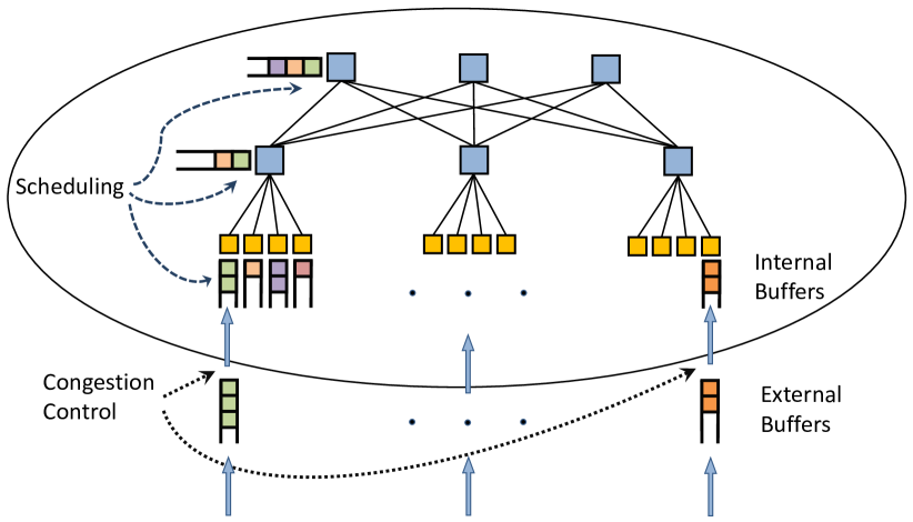
Figure 1: Overview of the congestion control and scheduling scheme.

Figure 2 illustrates our congestion control policy. The key idea is to view the system as a bandwidth sharing network with flow-level capacity constraints. The rate allocated to each flow buffered at source nodes is determined by an online algorithm that only uses the queue lengths of the external buffers, and satisfies the capacity constraints. Another key ingredient of our algorithm is a mechanism that translates the allocated rates to congestion control decisions. In particular, we implement the congestion control algorithm at the granularity of flows, as opposed to adjusting the rates on a packet-by-packet basis as in classical TCP.

We consider a specific bandwidth allocation scheme called the store-and-forward algorithm (SFA), which was first considered by Massoulié and later discussed in [7, 20, 35, 42]. The SFA policy has been shown to be insensitive with respect to general service time distributions [44], and result in a reversible network with Poisson arrival processes [42]. The bandwidth sharing network under SFA has a product-form queue size distribution in equilibrium. Given this precise description of the stationary distribution, we can obtain an explicit bound on the number of flows waiting at the source nodes, which has the desirable form of $O(\#\text{hops}\times\text{flow-size}/\text{gap-to-capacity})$. Details of the congestion control policy description and analysis are given in Section 4 to follow.

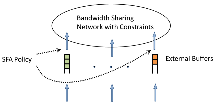
Figure 2: A congestion control policy based on the SFA algorithm for a bandwidth sharing network.

We also make use of the concept of emulation to design a packet scheduling algorithm in the internal network, which is operated in discrete time. In particular, we propose and analyze a scheduling mechanism that is able to emulate a continuous-time quasi-reversible network, which has a highly desirable queue-size scaling.

Our design consists of three elements. First, we specify the granularity of timeslot in a way that maintains the same throughput as in a network without the discretization constraint. By appropriately choosing the granularity, we are able to address a general setting where flows arriving on each route can have arbitrary sizes, as opposed to prior work that assumed unit-size flows. Second, we consider a continuous-time network operated under the Last-Come-First-Serve Preemptive-Resume (LCFS-PR) policy. If flows on each route are assumed to arrive according a Poisson process, the resulting queueing network is quasi-reversible with a product-form stationary distribution. In this continuous-time setting, we will show that the network achieves a flow delay bound of $O(\#\text{hops }\times\text{ flow-size }/\text{ gap-to-capacity})$. Finally, we design a feasible scheduling policy for the discrete-time network, which achieves the same throughput and delay bounds as the continuous-time network. The resulting scheduling scheme is illustrated in Figure 3.

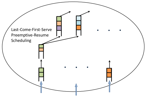
Figure 3: An adapted LCFS-PR scheduling algorithm

1.3 Our Contributions

The main contribution of the paper is a centralized policy for both congestion control and scheduling that achieves a per-flow end-to-end delay bound $O(\#\text{hops }\times$ $\text{flow-size }/\text{ gap-to-capacity})$. Some salient aspects of our result are:

1. The policy addresses both the congestion control and scheduling problems, in contrast to other previous work that focused on either congestion control or scheduling.

2. We consider flows with variable sizes.

3. We provide per-flow delay bound rather than an aggregate bound.

4. Our results are non-asymptotic, in the sense that they hold for any admissible load.

5. A central component of our design is the emulation of continuous-time quasi-reversible networks with a product-form stationary distribution. By emulating these queueing networks, we are able to translate the results therein to the network with congestion and scheduling constraints. This emulation result can be of interest in its own right.

1.4 Organization

The remaining sections of the paper are organized as follows. In Section 2 we describe the network model. The main results of the paper are presented in Section 3. The congestion control algorithm is described and analyzed in Section 4. Section 5 details the scheduling algorithm and its performance properties. We discuss implementation issues and conclude the paper in Section 6.

2 Model and Notation

In this section, we introduce our model. We consider multi-rooted tree topologies that have been widely adopted for datacenter networks [12, 2, 38]. Such tree topologies can be represented by a directed acyclic graph (DAG) model, to be described in detail shortly. We then describe the network dynamics based on the graph model. At a higher level, exogenous flows of various types arrive according to a continuous-time process. Each flow is associated with a route, and has some amount of data to be transferred along its route. As the internal network is operated in discrete time, i.e., time is slotted for unit-size packet transmission, each flow is broken into a number of packets. Packets of exogenous flows would be buffered at the source nodes upon arrival, and then injected into the internal network according a specified congestion control algorithm — an example being the classical TCP. The packets traverse along nodes on their respective routes, queueing in buffers at intermediate nodes. It is worth noting that a flow departs the network once all of its packets reach the destination.

2.1 An Acyclic Model

Before providing the construction of a directed acyclic graph model for the datacenter networks with tree topologies, we first introduce the following definition of dominance relation between two queues.

Definition 2.1 (Dominance relation).

For any two queues $Q_{1}$ and $Q_{2},$ $Q_{1}$ is said to be dominated by $Q_{2},$ denoted by $Q_{1}\preccurlyeq Q_{2},$ if there exists a flow for $Q_{2}$ such that its packets pass through $Q_{1}$ before entering $Q_{2}.$

For a datacenter with a tree topology, each node $v$ maintains two separate queues: a queue $Q_{v}^{u}$ that sends data “up” the tree, and another queue $Q_{v}^{d}$ that sends data “down” the tree. Here the notions of ”up” and ”down” are defined with respect to a fixed, chosen root of the tree — packets that are going towards nodes closer to the root are part of the “up” queue, while others are part of the “down” queue.

Consider the queues at leaf nodes of the tree. By definition, the up queues cannot dominate any other queues, and the down queues at leaf nodes cannot be dominated by any other queues. Therefore we can construct an order starting with the up queues at leaf nodes $\{v_{1},\ldots,v_{k}\}$, i.e., $Q_{v_{1}}^{u},\ldots,Q_{v_{k}}^{u}.$ The down queues at leaf nodes $Q_{v_{1}}^{d},\ldots,Q_{v_{k}}^{d}$ are placed at the end of the order. Now we can remove the leaf nodes and consider the remaining sub-tree. Inductively, we can place the up queues of layer-$l$ nodes right after the up queues of layer-$(l+1)$ nodes, and place the down queues of layer-$l$ nodes before those of layer-$(l+1)$ nodes. It is easy to verify that the resulting order gives a partial order of queues with respect to the dominance relation. Therefore, we can construct a directed acyclic graph for the tree topology, where each up/down queue $q_{i}$ is abstracted as a node. There exists a directed link from $q_{i}$ to $q_{j}$ if there exists a flow such that its packets are routed to $q_{j}$ right after departing $q_{i}.$

In the following, we represent the datacenter fabric by a directed acyclic graph $G(\mathcal{V},\mathcal{E}),$ where $\mathcal{V}$ is the node set, and $\mathcal{E}\subset\mathcal{V}\times\mathcal{V}$ is the set of directed links connecting nodes in $\mathcal{V}$. The graph is assumed to be connected. Let $N:=|\mathcal{V}|$ and $M:=|\mathcal{E}|$. Each entering flow is routed through the network from its source node to its destination node. There are $J$ classes of traffic routes indexed by $\mathcal{J}=\{1,2,\cdots,J\}$. Let notation $v\in j$ or $j\in v$ denote that route $j$ passes through node $v.$ We denote by $\boldsymbol{R}\in\mathbb{R}^{M\times J}$ the routing matrix of the network, which represents the connectivity of nodes in different routes. That is,

$$R_{mj}=\begin{cases}1,&\text{if route $j$ traverses link $m$}\\ 0,&\text{otherwise}.\end{cases}$$

2.2 Network Dynamics

Each flow is characterized by the volume of data to be transferred along its route, referred to as flow size. Note that the size of a flow remains constant when it passes through the network. The flow size set $\mathcal{X},$ which consists of all the sizes of flows arriving at the system, is assumed to be countable. Each flow can be classified according to its associated route and size, which defines the type of this flow. Let $\mathcal{T}:=\{(j,x):\;j\in\mathcal{J},\;x\in\mathcal{X}\}$ denote the set of flow types.

Flow arrivals. External flow arrivals occur according to a continuous-time stochastic process. The inter-arrival times of type-$(j,x)$ flows are assumed to be i.i.d. with mean $\frac{1}{\lambda_{j,x}}$ (i.e., with rate $\lambda_{j,x}$) and finite variance. Let $\boldsymbol{\lambda}=(\lambda_{j,x}:\;j\in\mathcal{J},\;x\in\mathcal{X})$ denote the arrival rate vector (of dimension $J|\mathcal{X}|$). We denote the traffic intensity of route $j$ by the notation $\alpha_{j}=\sum_{x\in\mathcal{X}}\;x\lambda_{j,x}.$ Let

$$f_{v}=\sum_{j:\;j\in v}\sum_{x\in\mathcal{X}}\;x\lambda_{j,x}$$

be the average service requirement for flows arriving at node $v$ per unit time. We define the effective load $\rho_{j}(\boldsymbol{\lambda})$ along the route $j$ as

$$\rho_{j}(\boldsymbol{\lambda})=\max_{v\in j}\;f_{v}.$$

As mentioned before, exogenous flows are queued at the external buffers upon arrival. The departure process of flows from the external buffer is determined by the congestion control policy. The flows are considered to have departed from the external buffer (not necessarily from the network though) as soon as the congestion control policy fully accepts it in the internal network for transmission.

Discretization. The internal network is operated in discrete time. Each flow is packetized. Packets of injected flows become available for transmission only at integral times, for instance, at the beginning of the timeslots. For a system with timeslot of length $\epsilon,$ a flow of size $x$ is decomposed into $\lceil\frac{x}{\epsilon}\rceil$ packets of equal size $\epsilon$ (the last packet may be of size less than a full timeslot). In a unit timeslot each node is allowed to transmit at most one $\epsilon$-size packet. If a node has less than a full timeslot worth of data to send, unused network bandwidth is left wasted. In order to eliminate bandwidth wastage and avoid throughput loss, the granularity of timeslot should be chosen appropriately (cf. Section 5).

Note that over a time interval $[k\epsilon,(k+1)\epsilon)$, the transmission of packets at nodes occurs instantly at time $k\epsilon,$ while the arrival of new flows to the network occurs continuously throughout the entire time interval.

2.2.1 Admissible Region without Discretization

By considering the network operating in continuous time without congestion control, we can characterize the admissible region of the network without discretization. Note that the service rate of each node is assumed to be deterministically equal to 1. We denote by $\boldsymbol{Q}(t)=(Q_{1}(t),Q_{2}(t),\ldots,Q_{N}(t))$ the queue-size vector at time $t\in[0,\infty),$ where $Q_{i}(t)$ is the number of flows at node $i.$ Note that the process $\boldsymbol{Q}(t)$ alone is not Markovian, since each flow size is deterministic and the interarrival times have a general distribution. We can construct a Markov description of the system, given by a process $\boldsymbol{Y}(t),$ by augmenting the queue-size vector $\boldsymbol{Q}(t)$ with the remaining size of the set of flows on each node, and the residual arrival times of flows of different types. The network system is said to be stable under a policy if the Markov process $\boldsymbol{Y}(t)$ is positive recurrent. An arrival rate vector is called (strictly) admissible if and only if the network with this arrival rate vector is stable under some policy. The admissible region of the network is defined as the set of all admissible arrival rate vectors.

Define a set ${\Lambda}\subset\mathbb{R}_{+}^{J|\mathcal{X}|}$ of arrival rate vectors as follows:

$${\Lambda}=\left\{\boldsymbol{\lambda}\in\mathbb{R}_{+}^{J|\mathcal{X}|}:\;f_{v}=\sum_{j:\;j\in v}\sum_{x\in\mathcal{X}}\;x\lambda_{j,x}<1,\forall v\in\mathcal{V}\right\}.$$ (2.1)

It is easy to see that if $\boldsymbol{\lambda}\notin{\Lambda},$ then the network is not stable under any scheduling policy, because in this case there exists at least one queue that receives load beyond its capacity. Therefore, the set ${\Lambda}$ contains the admissible region. As we will see in the subsequent sections, ${\Lambda}$ is in fact equal to the admissible region. In particular, for each $\boldsymbol{\lambda}$ in $\Lambda$, our proposed policy stabilizes the network with congestion control and discretization constraints.

2.3 Notation

The end-to-end delay of a flow refers to the time interval between the flow’s arrival and the moment that all of its packets reach the destination. We use $D^{(j,x),i}(\boldsymbol{\lambda})$ to denote the end-to-end delay of the $i$-th flow of size $x$ along route $j,$ for $j=1,\ldots,J,$ and $x\in\mathcal{X},$ under the joint congestion control and scheduling scheme, and the arrival rate vector $\boldsymbol{\lambda}.$ Note that $D^{(j,x),i}$ includes two parts: the time that a flow spends on waiting in the external buffer, denoted by $D_{W}^{(j,x),i},$ and the delay it experiences in the internal network, denoted by $D_{S}^{(j,x),i}.$ Then the sample mean of the waiting delay and that of the scheduling delay over all type-$(j,x)$ flows are:

$$D_{W}^{(j,x)}(\boldsymbol{\lambda}) =\limsup_{k\rightarrow\infty}\frac{1}{k}\sum_{i=1}^{k}D_{W}^{(j,x),i}(\boldsymbol{\lambda}),$$

$$D_{S}^{(j,x)}(\boldsymbol{\lambda}) =\limsup_{k\rightarrow\infty}\frac{1}{k}\sum_{i=1}^{k}D_{S}^{(j,x),i}(\boldsymbol{\lambda}).$$

When the steady state distributions exist, $D_{W}^{(j,x)}(\boldsymbol{\lambda})$ and $D_{S}^{(j,x)}(\boldsymbol{\lambda})$ are exactly the expected waiting delay and scheduling delay of a type-$(j,x)$ respectively. The expected total delay of a type-$(j,x)$ flow is:

$$D^{(j,x)}(\boldsymbol{\lambda})=D_{W}^{(j,x)}(\boldsymbol{\lambda})+D_{S}^{(j,x)}(\boldsymbol{\lambda}).$$

3 Main Results

In this section, we state the main results of our paper.

Theorem 3.1.

Consider a network described in Section 2 with a Poisson arrival rate vector $\boldsymbol{\lambda}\in\Lambda$. With an appropriate choice of time-slot granularity $\epsilon>0,$ there exists a joint congestion control and scheduling scheme for the discrete-time network such that for each flow type $(j,x)\in\mathcal{T}$,

$$D^{(j,x),\epsilon}(\boldsymbol{\lambda}) \leq C\left(\frac{xd_{j}}{1-\rho_{j}(\boldsymbol{\lambda})}+d_{j}\right)\quad\mbox{with probability}~{}1,$$

where $C>0$ is a universal constant.

The result stated in Theorem 3.1 holds for a network with an arbitrary acyclic topology. In terms of the delay bound, it is worth noting that a factor of the form $\frac{x}{1-\rho_{j}(\boldsymbol{\lambda})}$ is inevitable; in fact, the $\frac{1}{1-\rho}$ scaling behavior has been universally observed in a large class of queueing systems. For instance, consider a work-conserving $M/D/1$ queue where unit-size jobs or packets arrive as a Poisson process with rate $\rho<1$ and the server has unit capacity. Then, both average delay and queue-size scale as $1/(1-\rho)$ as $\rho\to 1$.

Additionally, the bounded delay implies that the system can be “stabilized” by properly choosing the timeslot granularity. In particular, our proposed algorithm achieves a desirable delay bound of

$$O(\#\text{hops }\times\text{ flow-size }/\text{ gap-to-capacity})$$

for any $\boldsymbol{\lambda}$ that is admissible. That is, system is throughput optimal as well.

Theorem 3.1 assumes that flows arrive as Poisson processes. The results can be extended to more general arrival processes with i.i.d. interarrival times with finite means, by applying the procedure of Poissonization considered in [10, 17]. This will lead to similar bounds as stated in Theorem 3.1 but with a (larger) constant $C$ that will also depend on the distributional characterization of the arrival process; see Section 6 for details.

Remark 3.2.

Consider the scenario that the size of flows on route $j$ has a distribution equal to a random variable $X_{i}.$ Then Theorem 3.1 implies that the expected delay for flows along route $j$ can be bounded as $D^{j,\epsilon}(\boldsymbol{\lambda})\leq C\left(\frac{\mathbb{E}[X_{j}]d_{j}}{1-\rho_{j}(\boldsymbol{\lambda})}+d_{j}\right).$

In order to characterize the network performance under the proposed joint scheme, we establish delay bounds achieved by the proposed congestion control policy and the scheduling algorithm, separately. The following theorems summarize the performance properties of our approach.

The first theorem argues that by using an appropriate congestion control policy, the delay of flows due to waiting at source nodes before getting ready for scheduling (induced by congestion control) is well behaved.

Theorem 3.3.

Consider a network described in Section 2 with a Poisson arrival rate vector $\boldsymbol{\lambda}\in\Lambda$, operating under the SFA congestion control policy described in Section 4. Then, for each flow type $(j,x)\in\mathcal{T}$, the per-flow waiting delay of type-$(j,x)$ flows is bounded as

$$D_{W}^{(j,x)}(\boldsymbol{\lambda}) \leq\frac{xd_{j}}{1-\rho_{j}(\boldsymbol{\lambda})},\quad\text{with probability}~{}1.$$

The second result is about scheduling variable length packets in the internal network in discrete time. If the network could operate in continuous time, arrival processes were Poisson and packet scheduling in the internal network were Last-Come-First-Serve Preemptive Resume (LCFS-PR), then the resulting delay would be the desired quantity due to the classical result about product-form stationary distribution of quasi-reversible queueing networks, cf. [5, 19]. However, in our setting, since network operates in discrete time, we cannot use LCFS-PR (or for that matter any of the quasi-reversible policies). As the main contribution of this paper, we show that there is a way to adapt LCFS-PR to the discrete time setting so that for each sample-path, the departure time of each flow is bounded above by its departure time from the ideal continuous-time network. Such a powerful emulation leads to Theorem 3.4 stated below. We note that [17] provided such an emulation scheme when all flows had the same (unit) packet size. Here we provide a generalization of such a scheme for the setting where variable flow sizes are present.

Theorem 3.4.

Consider a network described in Section 2 with a Poisson arrival rate vector $\boldsymbol{\lambda}\in\Lambda$, operating with an appropriate granularity of timeslot $\epsilon>0,$ under the adapted LCFS-PR scheduling policy to be described in Section 5. Then, for each $(j,x)\in\mathcal{T}$, the per-flow scheduling delay of type-$(j,x)$ flows is bounded as

$$D_{S}^{(j,x),\epsilon}(\boldsymbol{\lambda}) \leq C^{\prime}\left(\frac{xd_{j}}{1-\rho_{j}(\boldsymbol{\lambda})}+d_{j}\right)\quad\mbox{with probability}~{}1,$$

where $C^{\prime}>0$ is a universal constant.

As discussed, for Theorem 3.4 to be useful, it is essential to have the flow departure process from the first stage (i.e., the congestion control step) be Poisson. To that end, we state the following Lemma, which follows from an application of known results on the reversibility property of the bandwidth-sharing network under the SFA policy [42].

Lemma 3.5.

Consider the network described in Theorem 3.3. Then for each $(j,x)\in\mathcal{T},$ the departure times of type-$(j,x)$ flows form an independent Poisson process of rate $\lambda_{j,x}.$

Therefore, Theorem 3.1 is an immediate consequence of Theorems 3.3–3.4 and Lemma 3.5.

4 Congestion Control: An Adapted SFA Policy

In this section, we describe an online congestion control policy, and analyze its performance in terms of explicit bounds on the flow waiting time, as stated in Theorem 3.3 in Section 3. We start by describing the store-and-forward allocation policy (SFA) that is introduced in [35] and analyzed in generality in [7]. We describe its performance in Section 4.1. Section 4.2 details our congestion control policy, which is an adaptation of the SFA policy.

4.1 Store-and-Forward Allocation (SFA) Policy

We consider a bandwidth-sharing networking operating in continuous time. A specific allocation policy of interest is the store-and-forward allocation (SFA) policy.

Model. Consider a continuous-time network with a set $\mathcal{L}$ of resources. Suppose that each resource $l\in\mathcal{\mathcal{L}}$ has a capacity $C_{l}>0.$ Let $\mathcal{J}$ be the set of routes. Suppose that $|\mathcal{L}|=L$ and $|\mathcal{J}|=J$. Assume that a unit volume of flow on route $j$ consumes an amount $B_{lj}\geq 0$ of resource $l$ for each $l\in\mathcal{L},$ where $B_{lj}>0$ if $l\in j$, and $B_{lj}=0$ otherwise. The simplest case is where $B_{lj}\in\{0,1\},$ i.e., the matrix $B=(B_{lj},\;l\in\mathcal{L},\;j\in\mathcal{J})\in\mathbb{R}_{+}^{L\times J}$ is a $0$-$1$ incidence matrix. We denote by $\mathcal{\mathcal{K}}$ the set of all resource-route pairs $(l,j)$ such that route $j$ uses resource $l$, i.e., $\mathcal{K}=\left\{(l,j):\;B_{lj}>0\right\}$; assume that $|\mathcal{K}|=K.$

Flows arrive to route $j$ as a Poisson process of rate $\lambda_{i}$. For a flow of size $x$ on route $j$ arriving at time $t_{\text{start}},$ its completion time $t_{\text{end}}$ satisfies

$$x=\int_{t_{\text{start}}}^{t_{\text{end}}}c(t)dt,$$

where $c(t)$ is the bandwidth allocated to this flow on each link of route $j$ at time $t.$ The size of each flow on route $j$ is independent with distribution equal to a random variable $X_{j}$ with finite mean. Let $\mu_{j}=(\mathbb{E}[X_{j}])^{-1},$ and $\alpha_{j}=\frac{\lambda_{j}}{\mu_{j}}$ be the traffic intensity on route $j.$

Let $N_{j}(t)$ record the number of flows on route $j$ at time $t,$ and let $\boldsymbol{N}(t)=(N_{1}(t),N_{2}(t),\ldots,N_{J}(t)).$ Since the service requirement follows a general distribution, the queue length process $\boldsymbol{N}(t)$ itself is not Markovian. Nevertheless, by augmenting the queue-size vector $\boldsymbol{N}(t)$ with the residual workloads of the set of flows on each route, we can construct a Markov description of the system, denoted by a process $\boldsymbol{Z}(t).$ On average, $\alpha_{j}$ units of work arrive at route $j$ per unit time. Therefore, a necessary condition for the Markov process $\boldsymbol{Z}(t)$ to be positive recurrent is that

$$\sum_{j:\;l\in j}B_{lj}\alpha_{j}<C_{l},\quad\forall l\in\mathcal{L}.$$

An arrival rate vector $\boldsymbol{\lambda}=(\lambda_{j}:j\in\mathcal{J})$ is said to be admissible if it satisfies the above condition. Given an admissible arrival rate vector $\boldsymbol{\lambda},$ we can define the load on resource $l$ as

$$g_{l}(\boldsymbol{\lambda})=\left(\sum_{j:\;j\in l}B_{lj}\alpha_{j}\right)/C_{l}.$$

We focus on allocation polices such that the total bandwidth allocated to each route only depends on the current queue-size vector $\boldsymbol{n}=(n_{j}:\;j\in\mathcal{J})\in\mathbb{Z}_{+}^{J},$ which represents the number of flows on each route. We consider a processor-sharing policy, i.e., the total bandwidth $\phi_{j}$ allocated to route $j$ is equally shared between all $n_{j}$ flows. The bandwidth vector $\mathbf{\boldsymbol{\phi}}(\boldsymbol{n})=(\phi_{1}(\boldsymbol{n}),\ldots,\phi_{J}(\boldsymbol{n}))$ must satisfy the capacity constraints

$$\sum_{j:\;j\in l}B_{lj}\phi_{j}(\boldsymbol{n})\leq C_{l},\qquad\forall l\in\mathcal{L}.$$ (4.1)

Store-and-Forward Allocation (SFA) policy. The SFA policy was first considered by Massoulié (see page 63, Section 3.4.1 in [35]) and later analyzed in the thesis of Proutière [35]. It was shown by Bonald and Proutière [7] that the stationary distribution induced by this policy has a product form and is insensitive for phase-type service distributions. Later Zachary established its insensitivity for general service distributions [44]. Walton [42] and Kelly et al. [20] discussed the relation between the SFA policy, the proportionally fair allocation and multiclass queueing networks. Due to the insensitivity property of SFA, the invariant measure of the process $\boldsymbol{N}(t)$ only depends on the parameters $\boldsymbol{\lambda}$ and $\boldsymbol{\mu}.$

We introduce some additional notation to describe this policy. Given the vector $\boldsymbol{n}=(n_{j}:\;j\in\mathcal{J})\in\mathbb{Z}_{+}^{J},$ which represents the number of flows on each route, we define the set

$$U(\boldsymbol{n}) =\left\{\boldsymbol{m}=(m_{lj}:\;(l,j)\in\mathcal{K})\in\mathbb{Z}_{+}^{K}:\;n_{j}=\sum_{l:\;l\in j}m_{lj},\;\forall j\in\mathcal{J}\right\}.$$

With a slight abuse of notation, for each $\boldsymbol{m}\in\mathbb{Z}_{+}^{K},$ we define $m_{l}:=\sum_{j:\;l\in j}m_{lj}$ for all $l\in\mathcal{L}.$ We also define quantity

$${m_{l}\choose m_{lj}:\;j\ni l}=\frac{m_{l}!}{\prod_{j:\;l\in j}(m_{lj}!)}.$$

For $\boldsymbol{n}\in\mathbb{Z}_{+}^{J},$ let

$$\Phi(\boldsymbol{n})=\sum_{\boldsymbol{m}\in U(\boldsymbol{n})}\prod_{l\in\mathcal{L}}\left({m_{l}\choose m_{lj}:\;j\ni l}\prod_{j:\;l\in j}\left(\frac{B_{lj}}{C_{l}}\right)^{m_{lj}}\right).$$

We set $\Phi(\boldsymbol{n})=0$ if at least one of the components of $\boldsymbol{n}$ is negative.

The SFA policy assigns rates according to the function $\boldsymbol{\phi}:\mathbb{Z}_{+}^{J}\rightarrow\mathbb{R}_{+}^{J},$ such that for any $\boldsymbol{n}\in\mathbb{Z}_{+}^{J},$ $\boldsymbol{\phi}(\boldsymbol{n})=(\phi_{j}(\boldsymbol{n}))_{j=1}^{J},$ with

$$\phi_{j}(\boldsymbol{n})=\frac{\Phi(\boldsymbol{n}-\boldsymbol{e}_{j})}{\Phi(\boldsymbol{n})},$$

where $\boldsymbol{e}_{j}$ is the $j$-th unit vector in $\mathbb{Z}_{+}^{J}.$

The SFA policy described above has been shown to be feasible, i.e., $\boldsymbol{\phi}$ satisfies condition (4.1) [20, Corollary 2], [42, Lemma 4.1]. Moreover, prior work has established that the bandwidth-sharing network operating under the SFA policy has a product-form invariant measure for the number of waiting flows [7, 42, 20, 44], and the measure is insensitive to the flow size distributions [44, 42]. The above work is summarized in the following theorem [37, Theorem 4.1].

Theorem 4.1.

Consider a bandwidth-sharing network operating under the SFA policy described above. If

$$\sum_{j:\;l\in j}B_{lj}\alpha_{j}<C_{l},\quad\forall l\in\mathcal{L},$$

then the Markov process $\boldsymbol{Z}(t)$ is positive recurrent, and $\boldsymbol{N}(t)$ has a unique stationary distribution $\boldsymbol{\pi}$ given by

$$\boldsymbol{\pi}(\boldsymbol{n})=\frac{\Phi(\boldsymbol{n})}{\Phi}\prod_{j\in\mathcal{J}}\alpha_{j}^{n_{j}},\;\boldsymbol{n}\in\mathbb{Z}_{+}^{J},$$

where

$$\Phi=\prod_{l\in\mathcal{L}}\left(\frac{C_{l}}{C_{l}-\sum_{j:\;l\in j}B_{lj}\alpha_{j}}\right).$$

By using Theorem 4.1 (also see [37, Propositions 4.2 and 4.3]), an explicit expression can be obtained for $\mathbb{E}[N_{j}],$ the expected number of flows on each route.

Proposition 4.2.

Consider a bandwidth-sharing network operating under the SFA policy, with the arrival rate vector $\boldsymbol{\lambda}$ satisfying

$$\sum_{j:\;l\in j}B_{lj}\alpha_{j}<C_{l},\;\forall l\in\mathcal{L}.$$

For each $l\in\mathcal{L},$ let $g_{l}=\left(\sum_{j:\;l\in j}B_{lj}\alpha_{j}\right)/C_{l}.$ Then $\boldsymbol{N}(t)$ has a unique stationary distribution. In particular, for each $j\in\mathcal{J},$

$$\mathbb{E}[N_{j}]=\sum_{l:\;l\in j}\frac{B_{lj}\alpha_{j}}{C_{l}}\frac{1}{1-g_{l}}.$$

Proof.

Define a measure $\tilde{\boldsymbol{\pi}}$ on $\mathbb{Z}_{+}^{K}$ as follows [37, Proposition 4.2 ]: for each $\boldsymbol{m}\in\mathbb{Z}_{+}^{K},$

$$\tilde{\boldsymbol{\pi}}(\boldsymbol{m})=\frac{1}{\Phi}\prod_{l=1}^{L}\left({m_{l}\choose m_{lj}:\;j\ni l}\prod_{j:\;l\in j}\left(\frac{B_{lj}\alpha_{j}}{C_{l}}\right)^{m_{lj}}\right).$$

It has been shown that $\tilde{\boldsymbol{\pi}}$ is the stationary distribution for a multi-class network with processor sharing queues [20, Proposition 1], [42, Proposition 2.1]. Note that the marginal distribution of each queue in equilibrium is the same as if the queue were operating in isolation. To be precise, for each queue $l,$ the queue size is distributed as if the queue has Poisson arrival process of rate $g_{l}.$ Hence the size of queue $l,$ denoted by $M_{l},$ satisfies $\mathbb{E}_{\tilde{\boldsymbol{\pi}}}[M_{l}]=\frac{g_{l}}{1-g_{l}}.$ Let $M_{lj}$ be the number of class $j$ customers at queue $l.$ Then by Theorem 3.10 in [19], we have

$$\mathbb{E}_{\tilde{\boldsymbol{\pi}}}[M_{lj}]=\frac{B_{lj}\alpha_{j}}{\sum_{i:\;l\in i}B_{li}\alpha_{i}}\mathbb{E}_{\tilde{\boldsymbol{\pi}}}[M_{l}]=\frac{B_{lj}\alpha_{j}}{C_{l}}\frac{1}{1-g_{l}}.$$ (4.2)

Given the above expressions of $\tilde{\boldsymbol{\pi}}$ and $\boldsymbol{\pi}$, we can show that $\boldsymbol{\pi}(\boldsymbol{n})=\sum_{\boldsymbol{m}\in U(\boldsymbol{n})}\tilde{\boldsymbol{\pi}}(\boldsymbol{m}),$ $\forall\boldsymbol{n}\in\mathbb{Z}_{+}^{J}$. This fact has been shown by Bonald and Proutière [8] and Walton [42]. Hence we have

$$\mathbb{E}_{\boldsymbol{\pi}}[N_{j}] =\sum_{k=0}^{\infty}k\left(\sum_{\boldsymbol{n}\in\mathbb{Z}_{+}^{J}:n_{j}=k}\boldsymbol{\pi}(\boldsymbol{n})\right)=\sum_{k=0}^{\infty}k\left(\sum_{\boldsymbol{n}\in\mathbb{Z}_{+}^{J}:n_{j}=k}\sum_{\boldsymbol{m}\in U(\boldsymbol{n})}\tilde{\boldsymbol{\pi}}(\boldsymbol{m})\right)$$

$$=\sum_{k=0}^{\infty}k\left(\sum_{\boldsymbol{m}\in\mathbb{Z}_{+}^{K}}\mathbb{I}(\sum_{l:\;l\in j}m_{lj}=k)\tilde{\boldsymbol{\pi}}(\boldsymbol{m})\right)$$

$$=\mathbb{E}_{\tilde{\boldsymbol{\pi}}}\Big{[}\sum_{l:\;l\in j}M_{lj}\Big{]}$$

$$=\sum_{l:\;l\in j}\frac{B_{lj}\alpha_{j}}{C_{l}}\frac{1}{1-g_{l}}$$

as desired. ∎

We now consider the departure processes of the bandwidth-sharing network. It is a known result that the bandwidth sharing network with the SFA policy is reversible, as summarized in the proposition below. This fact has been observed by Proutière [35], Bonald and Proutière [8], and Walton [42]. Note that Lemma 3.5 follows immediately from the reversibility property of the network and the fact that flows of each type arrive according to a Poisson process.

Proposition 4.3 (Proposition 4.2 in [42]).

Consider a bandwidth sharing network operating under SFA. If $\sum_{j:\;l\in j}B_{lj}\alpha_{j}<C_{l},\;\forall l\in\mathcal{L},$ then the network is reversible.

4.2 An SFA-based Congestion Control Scheme

We now describe a congestion control scheme for a general acyclic network. As mentioned earlier, every exogenous flow is pushed to the corresponding external buffer upon arrival. The internal buffers store flows that are either transmitted from other nodes or moved from the external buffers. We want to emphasize that only packets present in the internal queues are eligible for scheduling. The congestion control mechanism determines the time at which each external flow should be admitted into the network for transmission, i.e., when a flow is removed from the external buffer and pushed into the respective source internal buffer.

The key idea of our congestion control policy is as follows. Consider the network model described in Section 2, denoted by $\mathcal{N}$. Let $A$ be an $N\times J$ matrix where

$$A_{nj}=\begin{cases}1,&\text{if route $j$ passes through node $n$}\\ 0,&\text{otherwise.}\end{cases}$$

The corresponding admissible region $\Lambda$ given by (2.1) can be equivalently written as

$$\Lambda=\left\{\boldsymbol{\lambda}\in\mathbb{R}_{+}^{J|\mathcal{X}|}:\;A\boldsymbol{\alpha}<\boldsymbol{1}\right\},$$

where $\boldsymbol{\alpha}=(\alpha_{j},\;j\in\mathcal{J})$ with $\alpha_{j}:=\sum_{x\in\mathcal{X}}\;x\lambda_{j,x},$ and $\boldsymbol{1}$ is an $N$-dim vector with all elements equal to one.

Now consider a virtual bandwidth-sharing network, denoted by $\mathcal{N}_{B}$, with $J$ routes which have a one-to-one correspondence with the $J$ routes in $\mathcal{N}$. The network $\mathcal{N}_{B}$ has $N$ resources, each with unit capacity. The resource-route relation is determined precisely by the matrix $A.$ Observe that each resource in $\mathcal{N}_{B}$ corresponds to a node in $\mathcal{N}.$ Assume that the exogenous arrival traffic of $\mathcal{N}_{B}$ is identical to that of $\mathcal{N}$. That is, each flow arrives at the same route of $\mathcal{N}$ and $\mathcal{N}_{B}$ at the same time. $\mathcal{N}_{B}$ will operate under the insensitive SFA policy described in Section 4.1.

Emulation scheme $E$. Flows arriving at $\mathcal{N}$ will be admitted into the network for scheduling in the following way. For a flow $f$ arriving at its source node $v_{s}$ at time $t_{f}$, let $\delta_{f}$ denote its departure time from $\mathcal{N}_{B}$. In the network $\mathcal{N},$ this flow will be moved from the external buffer to the internal queue of node $v_{s}$ at time $\delta_{f}.$ Then all packets of this flow will simultaneously become eligible for scheduling. Conceptually, all flows will be first fed into the virtual network $\mathcal{N}_{B}$ before being admitted to the internal network for transmission.

This completes the description of the congestion control policy. Observe that the centralized controller simulates the virtual network $\mathcal{N}_{B}$ with the SFA policy in parallel, and tracks the departure processes of flows in $\mathcal{N}_{B}$ to make congestion control decisions for $\mathcal{N}$. According to the above emulation scheme $E$, we have the following lemma.

Lemma 4.4.

Let $D_{B}$ denote the delay of a flow $f$ in $\mathcal{N}_{B},$ and $D_{W}$ be the amount of time the flow spends at the external buffer in $\mathcal{N}$. Then $D_{W}=D_{B}$ surely.

For each flow type $(j,x)\in\mathcal{T},$ let $D_{B}^{(j,x)}(\boldsymbol{\lambda})$ denote the sample mean of the delays over all type-$(j,x)$ flows in the bandwidth sharing network $\mathcal{N}_{B}.$ That is, $D_{B}^{(j,x)}(\boldsymbol{\lambda}):=\limsup_{k\rightarrow\infty}\frac{1}{k}\sum_{i=1}^{k}D_{B}^{(j,x),i}(\boldsymbol{\lambda}),$ where $D_{B}^{(j,x),i}(\boldsymbol{\lambda})$ is the delay of the $i$-th type-$(j,x)$ flow. From Theorem 4.1 and Proposition 4.2, we readily deduce the following result.

Proposition 4.5.

In the network $\mathcal{\mathcal{N}}_{B},$ we have

$$D_{B}^{(j,x)}(\boldsymbol{\lambda})=\sum_{v:v\in j}\frac{x}{1-f_{v}},\quad\text{with probability $1.$}$$

Proof.

Recall that in the network $\mathcal{N}_{B},$ flows arriving on each route are further classified by the size. Each type-$(j,x)$ flow requests $x$ amount of service, deterministically. It is not difficult to see that properties of the bandwidth-sharing network stated in Section 4.1 still hold with the refined classification. We denote by $N_{j,x}(t)$ the number of type-$(j,x)$ flows at time $t.$ A Markovian description of the system is given by a process $\boldsymbol{Z}(t)$, whose state contains the queue-size vector $\boldsymbol{N}(t)=(N_{j,x}(t),j\in\mathcal{J},x\in\mathcal{X})$ and the residual workloads of the set of flows on each route.

By construction, each resource $v$ in the network $\mathcal{N}_{B}$ corresponds to a node $v$ in the network $\mathcal{N},$ with unit capacity. The load $g_{v}$ on the resource $v$ of $\mathcal{N}_{B}$ and the load $f_{v}$ on node $v$ of $\mathcal{N}$ satisfy the relationship

$$g_{v}=\sum_{v:v\in j}A_{vj}\alpha_{j}=f_{v}.$$

As $\boldsymbol{\lambda}\in\Lambda,$ $f_{v}<1$ for each $v\in\mathcal{V}.$ By Theorem 4.1, the Markov process $\boldsymbol{Z}(t)$ is positive recurrent, and $\boldsymbol{N}(t)$ has a unique stationary distribution. Let $N_{j,x}$ denote the number of type-$(j,x)$ flow in the bandwidth sharing network $\mathcal{N}_{B}$, in equilibrium. Following the same argument as in the proof of Proposition 4.2, we have

$$\mathbb{E}[N_{j,x}]=\sum_{v:\;v\in j}\frac{x\lambda_{j,x}}{1-f_{v}}.$$

Consider the delay of a type-$(j,x)$ flow in equilibrium, denoted by $\bar{D}_{B}^{(j,x)}(\boldsymbol{\lambda})$. By applying Little’s Law to the stationary system concerning only type-$(j,x)$ flows, we can obtain

$$\mathbb{E}[\bar{D}_{B}^{(j,x)}(\boldsymbol{\lambda})]=\frac{\mathbb{E}[N_{j,x}]}{\lambda_{j,x}}=\sum_{v:\;v\in j}\frac{x}{1-f_{v}}.$$

By the ergodicity of the network $\mathcal{N}_{B},$ we have

$$D_{B}^{(j,x)(\boldsymbol{\lambda})}=\mathbb{E}[\bar{D}_{B}^{(j,x)}(\boldsymbol{\lambda})],\quad\text{with probability}\;1,$$

thereby completing the proof of Proposition 4.5. ∎

Equipped with Proposition 4.5 and Lemma 4.4, we are now ready to prove Theorem 3.3.

Proof of Theorem 3.3.

By the definition, we have $\frac{1}{1-f_{v}}\leq\frac{1}{1-\rho_{j}(\boldsymbol{\lambda})}$, for each $v\in j.$ Proposition 4.5 implies that, with probability 1,

$$D_{B}^{(j,x)}(\boldsymbol{\lambda})=\sum_{v:v\in j}\frac{x}{1-f_{v}}\leq\frac{xd_{j}}{1-\rho_{j}(\boldsymbol{\lambda})},$$

It follows from Lemma 4.4 that $D_{W}^{(j,x)}(\boldsymbol{\lambda})=D_{B}^{(j,x)}(\boldsymbol{\lambda}).$ Therefore, we have

$$D_{W}^{(j,x)}(\boldsymbol{\lambda})\leq\frac{xd_{j}}{1-\rho_{j}(\boldsymbol{\lambda})},\quad\text{with probability}\;1.$$

This completes the proof of Theorem 3.3. ∎

5 Scheduling: Emulating LCFS-PR

In this section, we design a scheduling algorithm that achieves a delay bound of

$$O\Big{(}\#\text{hops}\times\text{flow-size}\times\frac{1}{\text{gap-to-capacity}}\Big{)}$$

without throughput loss for a multi-class queueing network operating in discrete time. As mentioned earlier, our design consists of three key steps. We first discuss how to choose the granularity of time-slot $\epsilon$ appropriately, in order to avoid throughput loss in the discrete-time network. In terms of the delay bound, we leverage the results from a continuous-time network operating under the Last-Come-First-Serve Preemptive-Resume (LCFS-PR) policy. With a Poisson arrival process, the network becomes quasi-reversible with a product-form stationary distribution. Then we adapt the LCFS-PR policy to obtain a scheduling scheme for the discrete-time network. In particular, we design an emulation scheme such that the delay of a flow in the discrete-time network is bounded above by the delay of the corresponding flow in the continuous-time network operating under LCFS-PR. This establishes the delay property of the discrete-time network.

5.1 Granularity of Discretization

We start with the following definitions that will be useful going forward.

Definition 5.1 ($\mathcal{N}_{D}^{(\epsilon)}$ network).

It is a discrete-time network with the topology, service requirements and exogenous arrivals as described in Section 2. In particular, each time slot is of length $\epsilon$. Additionally, the arrivals of size-$x$ flows on route $j$ form a Poisson process of rate $\lambda_{j,x}.$ For such a type-$(j,x)$ flow, its size in $\mathcal{N}_{D}^{(\epsilon)}$ becomes

$$x^{(\epsilon)}:=\epsilon\left\lceil\frac{x}{\epsilon}\right\rceil,$$

and the flow is decomposed into $\lceil\frac{x}{\epsilon}\rceil$ packets of equal size $\epsilon$.

Definition 5.2 ($\mathcal{N}_{C}^{(\epsilon)}$ network).

It is a continuous-time network with the same topology, service requirements and exogenous arrivals as $\mathcal{N}_{D}^{(\epsilon)}.$ The size of a type-$(j,x)$ flow is modified in the same way as that in $\mathcal{N}_{D}^{(\epsilon)}$.

Consider the network $\mathcal{N}_{D}^{(\epsilon)}.$ Given an arrival rate vector $\boldsymbol{\lambda}\in\Lambda,$ the load on node $v$ is

$$f_{v}^{(\epsilon)}= \sum_{j:j\in v}\sum_{x:x\in\mathcal{X}}\epsilon\left\lceil\frac{x}{\epsilon}\right\rceil\lambda_{j,x}.$$

As each node has a unit capacity, $\boldsymbol{\lambda}$ is admissible in $\mathcal{N}_{D}^{(\epsilon)}$ only if $f_{v}^{(\epsilon)}<1$ for all $v\in\mathcal{V}$. We let

$$\epsilon =\min\left\{\frac{1}{C_{0}}\cdot\min_{v\in\mathcal{V}}\left\{\frac{1-f_{v}}{\sum_{j:j\in v}\sum_{x:x\in\mathcal{X}}\lambda_{j,x}}\right\},\;\min_{j\in\mathcal{J}}\left\{1-\rho_{j}(\boldsymbol{\lambda})\right\}\right\},$$ (5.1)

where $C_{0}>1$ is an arbitrary constant. Then for each $v\in\mathcal{V},$

$$f_{v}^{(\epsilon)} <\sum_{j:j\in v}\sum_{x:x\in\mathcal{X}}(x+\epsilon)\lambda_{j,x}$$

$$=f_{v}+\epsilon\sum_{j:j\in v}\sum_{x:x\in\mathcal{X}}\lambda_{j,x}$$

$$\overset{(a)}{\leq}f_{v}+\frac{1-f_{v}}{C_{0}},$$

where the inequality (a) holds because $\epsilon\leq\frac{1-f_{v}}{C_{0}}\cdot\frac{1}{\sum_{j:j\in v}\sum_{x:x\in\mathcal{X}}\lambda_{j,x}}$ by the definition of $\epsilon$ in Eq. (5.1). Since $\boldsymbol{\lambda}\in\Lambda,$ for each $v\in\mathcal{V},$ $f_{v}<1$. We thus have

$$1-f_{v}^{(\epsilon)}\geq\frac{C_{0}-1}{C_{0}}(1-f_{v})>0.$$ (5.2)

Thus, each $\boldsymbol{\lambda}\in\Lambda$ is admissible in the discrete-time network $\mathcal{N}_{D}^{(\epsilon)}$.

5.2 Property of $\mathcal{N}_{C}^{(\epsilon)}$

Consider the continuous-time open network $\mathcal{N}_{C}^{(\epsilon)}$, where a LCFS-PR scheduling policy is used at each node. From Theorems $3.7$ and $3.8$ in [19], the network $\mathcal{N}_{C}^{(\epsilon)}$ has a product-form queue length distribution in equilibrium, if the following conditions are satisfied:

1. the service time distribution is either phase-type or the limit of a sequence of phase-type distributions;

2. the total traffic at each node is less than its capacity.

Note that the sum of $n$ exponential random variables each with mean $\frac{1}{nx}$ has a phase-type distribution and converges in distribution to a constant $x,$ as $n$ approaches infinity. Thus the first condition is satisfied. For each $\boldsymbol{\lambda}\in\Lambda,$ the second condition holds for $\mathcal{N}_{C}^{(\epsilon)}$ with $\epsilon$ defined as Eq. (5.1).

In the following theorem, we establish a bound for the delay experience by each flow type. For $j\in\mathcal{J},x\in\mathcal{X},$ let $D^{(j,x),\epsilon}(\boldsymbol{\lambda})$ denote the sample mean of the delay over all type-$(j,x)$ flows, i.e.,

$$D^{(j,x),\epsilon}(\boldsymbol{\lambda}) =\limsup_{k\rightarrow\infty}\frac{1}{k}\sum_{i=1}^{k}D^{(j,x),\epsilon,i}(\boldsymbol{\lambda}),$$

where $D^{(j,x),\epsilon,i}$ is the delay of the $i$-th type-$(j,x)$ flow.

Theorem 5.3.

In the network $\mathcal{N}_{C}^{(\epsilon)},$ we have

$${D}^{(j,x),\epsilon}(\boldsymbol{\lambda})=\sum_{v:v\in j}\frac{x^{(\epsilon)}}{1-f_{v}^{(\epsilon)}},\quad\mbox{with probability }1.$$

Proof.

The network $\mathcal{N}_{C}^{(\epsilon)}$ described above is an open network with Poisson exogenous arrival processes. An LCFS-PR queue management is used at each node in $\mathcal{N}_{C}^{(\epsilon)}.$ The service requirement of each flow at each node is deterministic with bounded support. As shown in [19] (see Theorem 3.10 of Chapter 3), the network $\mathcal{N}_{C}^{(\epsilon)}$ is an open network of quasi-reversible queues. Therefore, the queue size distribution of $\mathcal{N}_{C}^{(\epsilon)}$ has a product form in equilibrium. Further, the marginal distribution of each queue in equilibrium is the same as if the queue is operating in isolation. Consider a node $v.$ We denote by $Q_{v}$ the queue size of node $v$ in equilibrium. In isolation, $Q_{v}$ is distributed as if the queue has a Poisson arrival process of rate $f_{v}^{(\epsilon)}.$ Theorem $3.10$ implies that the queue is quasi-reversible and hence it has a distribution such that

$$\mathbb{E}[Q_{v}]=\frac{f_{v}^{(\epsilon)}}{1-f_{v}^{(\epsilon)}}.$$

Let $Q_{v}^{(j,x)}$ denote the number of type-$(j,x)$ flows at node $v$ in equilibrium. Note that $x^{(\epsilon)}\lambda_{j,x}$ is the average amount of service requirement for type-$(j,x)$ flows at node $v$ per unit time. Then by Theorem $3.10$ [19], we have

$$\mathbb{E}[Q_{v}^{(j,x)}]=\frac{x^{(\epsilon)}\lambda_{j,x}}{f_{v}^{(\epsilon)}}\mathbb{E}[Q_{v}].$$

Let $\bar{D}_{v}^{(j,x),\epsilon}(\boldsymbol{\lambda})$ denote the delay experienced by a type-$(j,x)$ flow at node $v,$ in equilibrium. Applying Little’s Law to the stable system concerning only type-$(j,x)$ flows at node $v$, we can obtain

$$\mathbb{E}[\bar{D}_{v}^{(j,x),\epsilon}(\boldsymbol{\lambda})]=\frac{\mathbb{E}[Q_{v}^{(j,x)}]}{\lambda_{j,x}}=\frac{x^{(\epsilon)}}{1-f_{v}^{(\epsilon)}}.$$

Therefore, the delay experienced by a flow of size $x$ along the entire route $j,$ $\bar{D}^{(j,x),\epsilon}(\boldsymbol{\lambda}),$ satisfies

$$\mathbb{E}[\bar{D}^{(j,x),\epsilon}(\boldsymbol{\lambda})]=\sum_{v:v\in j}\mathbb{E}[\bar{D}_{v}^{(j,x),\epsilon}(\boldsymbol{\lambda})]=\sum_{v:v\in j}\frac{x^{(\epsilon)}}{1-f_{v}^{(\epsilon)}}.$$

By the ergodicity of the network $\mathcal{N}_{C}^{(\epsilon)},$ with probability 1,

$${D}^{(j,x),\epsilon}(\boldsymbol{\lambda})=\mathbb{E}[\bar{D}^{(j,x),\epsilon}(\boldsymbol{\lambda})]=\sum_{v:v\in j}\frac{x^{(\epsilon)}}{1-f_{v}^{(\epsilon)}}.$$

∎

5.3 Scheduling Scheme for $\mathcal{N}_{D}^{(\epsilon)}$

In the discrete-time networks, each flow is packetized and time is slotted for packetized transmission. The scheduling policy for $\mathcal{N}_{D}^{(\epsilon)}$ differs from that for $\mathcal{N}_{C}^{(\epsilon)}$ in the following ways:

1. A flow/packet generated at time $t$ becomes eligible for transmission only at the $\lceil\frac{t}{\epsilon}\rceil$-th time slot;

2. A complete packet has to be transmitted in a time slot, i.e., fractions of packets cannot be transmitted.

Therefore, the LCFS-PR policy in $\mathcal{N}_{C}^{(\epsilon)}$ cannot be directly implemented. We need to adapt the LCFS-PR policy to our discrete-time setting. The adaption was first introduced by El Gamal et al. [10] and has been applied to the design of a scheduling algorithm for a constrained network [17]. However, it was restricted to the setup where all flows had unit size. Unlike that, here we consider variable size flows. Before presenting the adaptation of LCFS-PR scheme, we first make the following definition.

Definition 5.4 (Flow Arrival Time in $\mathcal{N}_{D}^{(\epsilon)}$).

The arrival time of a flow at a node $v$ in $\mathcal{N}_{D}^{(\epsilon)}$ is defined as the arrival time of its last packet at node $v$. That is, assume that its $i$-th packet arrives at node $v$ at time $p_{i},$ then the flow is said to arrive at node $v$ at time $A=\max_{1\leq i\leq k}p_{i}.$ Similarly, we define the departure time of a flow from a node as the moment when its last packet leaves this node.

Emulation scheme. Suppose that exogenous flows arrive at $\mathcal{N}_{C}^{(\epsilon)}$ and $\mathcal{N}_{D}^{(\epsilon)}$ simultaneously. In $\mathcal{N}_{C}^{(\epsilon)}$, flows are served at each node according to the LCFS-PR policy. For $\mathcal{N}_{D}^{(\epsilon)},$ we consider a scheduling policy where packets of a flow will not be eligible for transmission until the full flow arrives. Let the arrival time of a flow at some node in $\mathcal{N}_{C}$ be $\tau$ and in $\mathcal{N}_{D}^{(\epsilon)}$ at the same node be $A.$ Then packets of this flow are served in $\mathcal{N}_{D}^{(\epsilon)}$ using an LCFS-PR policy with the arrival time $\epsilon\lceil\frac{\tau}{\epsilon}\rceil$ instead of $A.$ If multiple flows arrive at a node at the same time, the flow with the largest arrival time in $\mathcal{N}_{C}^{(\epsilon)}$ is scheduled first. For a flow with multiple packets, packets are transmitted in an arbitrary order.

This scheduling policy is feasible in $\mathcal{N}_{D}^{(\epsilon)}$ if and only if each flow arrives before its scheduled departure time, i.e., $A\leq\epsilon\lceil\frac{\tau}{\epsilon}\rceil$ for every flow at each node. Let $\delta$ and $\Delta$ be the departure times of a flow from some node in $\mathcal{N}_{C}^{(\epsilon)}$ and $\mathcal{N}_{D}^{(\epsilon)}$, respectively. Since the departure time of a flow at a node is exactly its arrival time at the next node on the route, it is sufficient to show that $\Delta\leq\epsilon\lceil\frac{\delta}{\epsilon}\rceil$ for each flow in every busy cycle of each node in $\mathcal{N}_{C}^{(\epsilon)}.$ This will be proved in the following lemma.

Lemma 5.5.

Assume that a flow departs from a node in $\mathcal{N}_{C}^{(\epsilon)}$ and $\mathcal{N}_{D}^{(\epsilon)}$ at times $\delta$ and $\Delta,$ respectively. Then $\Delta\leq\epsilon\lceil\frac{\delta}{\epsilon}\rceil.$

Proof.

As the underlying graph $\mathcal{G}$ for $\mathcal{N}_{C}^{(\epsilon)}$ and $\mathcal{N}_{D}^{(\epsilon)}$ is a DAG, there is a topological ordering of the vertices $\mathcal{V}.$ Without loss of generosity, assume that $v_{1},\ldots,v_{n}$ is a topological order of $\mathcal{G}.$ We prove the statement via induction on the index of vertex.

Base case. We show that the statement holds for node $v_{1},$ i.e., $\Delta\leq\epsilon\lceil\frac{\delta}{\epsilon}\rceil$ for each flow in every busy cycle of node $v_{1}.$ We do so via induction on the number $k$ of flows that contribute to the busy cycle of node $v_{1}$ in $\mathcal{N}_{C}^{(\epsilon)}.$ Consider a busy cycle consisting of flows numbered $1,\ldots,k$ with arrivals at times $\tau_{1}\leq\ldots\leq\tau_{k}$ and departures at times $\delta_{1},\ldots,\delta_{k}.$ We denote by $c_{i}=(j_{i},x_{i})$ the type of flow numbered $i.$ Let the arrival times of these flows at node $v_{1}$ in $\mathcal{N}_{D}^{(\epsilon)}$ be $A_{1},\ldots,A_{k}$ and departures at times $\Delta_{1},\ldots,\Delta_{k}.$ As the first node in the topological ordering, node $v_{1}$ only has external arrivals. Hence $A_{i}=\epsilon\lceil\frac{\tau_{i}}{\epsilon}\rceil$ for $i=1,\ldots,k$. We need to show that $\Delta_{i}\leq\epsilon\lceil\frac{\delta_{i}}{\epsilon}\rceil,$ for $i=1,\ldots,k.$ For brevity, we let $S_{i}$ denote the schedule time for the $i$-th flow in $\mathcal{N}_{D}^{(\epsilon)}.$ We have $S_{i}=\epsilon\lceil\frac{\tau_{i}}{\epsilon}\rceil.$

Nested base case. For $k=1,$ since this busy cycle consists of only one flow of type $(j_{1},x_{1}),$ no arrival will occur at this node until the departure of this particular flow. In other words, for each flow that arrives at node $v_{1}$ after time $\tau_{1},$ its arrival time, denoted by $\tau_{f},$ should satisfy $\tau_{f}\geq\tau_{1}+x_{1}^{(\epsilon)}.$ Thus $A_{f}\leq\epsilon\left\lceil\frac{\tau_{f}}{\epsilon}\right\rceil,$ and the schedule time for flow $f$ in $\mathcal{N}_{D}^{(\epsilon)}$ should satisfy

$$S_{f}=\epsilon\left\lceil\frac{\tau_{f}}{\epsilon}\right\rceil\geq\epsilon\left(\left\lceil\frac{\tau_{1}}{\epsilon}\right\rceil+\frac{x_{1}^{(\epsilon)}}{\epsilon}\right).$$

Hence in $\mathcal{N}_{D}^{(\epsilon)}$, flow $f$ will not become eligible for service until node $v_{1}$ transmits all packets of the flow 1. Therefore, $\Delta_{1}=S_{1}+x_{1}^{(\epsilon)}=\epsilon\left\lceil\frac{\delta_{1}}{\epsilon}\right\rceil.$ Thus the induction hypothesis is true for the base case.

Nested induction step. Now assume that the bound $\Delta\leq\epsilon\lceil\frac{\delta}{\epsilon}\rceil$ holds for all busy cycles consisting of $k$ flows at $v_{1}$ in $\mathcal{N}_{C}^{(\epsilon)}$. Consider a busy cycle of $k+1$ flows.

Note that in $\mathcal{N}_{C}^{(\epsilon)},$ the LCFS-PR service policy determines that the first flow of the busy cycle is the last to depart. That is, $\delta_{1}=\tau_{1}+\sum_{i=1}^{k+1}x_{i}^{(\epsilon)}.$ Since flow $i$ is in the same busy cycle of flow $1$ in $\mathcal{N}_{C}^{(\epsilon)},$ its arrival time should satisfy $\tau_{i}<\tau_{1}+\sum_{l=1}^{i-1}x_{l}^{(\epsilon)},$ for $i=2,\ldots,k+1.$ Thus $\left\lceil\frac{\tau_{i}}{\epsilon}\right\rceil\leq\left\lceil\frac{\tau_{1}}{\epsilon}\right\rceil+\sum_{l=1}^{i-1}\frac{x_{l}^{(\epsilon)}}{\epsilon},$ i.e., $S_{i}\leq S_{1}+\sum_{l=1}^{i-1}x_{l}^{(\epsilon)}.$ Let us focus on the departure times of these flows in $\mathcal{N}_{D}^{(\epsilon)}.$

Case (i): There exists some $i$ such that $S_{i}=S_{1}+\sum_{l=1}^{i-1}x_{l}^{(\epsilon)}.$ Let $i^{*}$ be the smallest $i$ satisfying this equality. Then under the LCFS-PR policy in $\mathcal{N}_{D}^{(\epsilon)},$ the $i^{*}$-th flow will be scheduled for service right after the departure of flow $1.$ That is, $\Delta_{1}=S_{1}+\sum_{l=1}^{i^{*}-1}x_{l}^{(\epsilon)}=\epsilon\left\lceil\frac{\tau_{1}}{\epsilon}\right\rceil+\sum_{l=1}^{i^{*}-1}x_{l}^{(\epsilon)}\leq\epsilon\left\lceil\frac{\tau_{1}}{\epsilon}\right\rceil+\sum_{l=1}^{k+1}x_{l}^{(\epsilon)}=\epsilon\left\lceil\frac{\delta_{1}}{\epsilon}\right\rceil.$ The remaining flows numbered $i^{*},\ldots,k+1$ depart exactly as if they belong to a busy cycle of $k+2-i^{*}$ flows.

Case (ii): For $i=2,\ldots,k+1,$ $S_{i}<S_{1}+\sum_{l=1}^{i-1}x_{l}^{(\epsilon)}.$ Then with the LCFS-PR policy in $\mathcal{N}_{D}^{(\epsilon)},$ flows numbered $2,\ldots,k+1$ would have departure times as if they are from a busy cycle of $k$ flows. The service for flow $1$ will be resumed after the departure of these $k$ flows. In particular, we will show that the resumed service for flow $1$ will not be interrupted by any further arrival. Then $\Delta_{1}=S_{1}+\sum_{l=1}^{k+1}x_{l}^{(\epsilon)}=\epsilon\left\lceil\frac{\tau_{1}}{\epsilon}\right\rceil+\sum_{l=1}^{k+1}x_{l}^{(\epsilon)}=\epsilon\left\lceil\frac{\delta_{1}}{\epsilon}\right\rceil.$

Since this particular busy cycle in $\mathcal{N}_{C}^{(\epsilon)}$ consists of $k+1$ flows, arguing similarly as the base case, each flow $f$ that arrives at node $v_{1}$ after this busy cycle should satisfy $\tau_{f}\geq\delta_{1}.$ Hence its schedule time $S_{f}$ in $\mathcal{N}_{D}^{(\epsilon)}$ satisfies $S_{f}=\epsilon\left\lceil\frac{\tau_{f}}{\epsilon}\right\rceil\geq\epsilon\left\lceil\frac{\delta_{1}}{\epsilon}\right\rceil=\epsilon\left\lceil\frac{\tau_{1}}{\epsilon}\right\rceil+\sum_{l=1}^{k+1}x_{l}^{(\epsilon)}=S_{1}+\sum_{l=1}^{k+1}x_{l}^{(\epsilon)}.$ Therefore, flow $f$ will not be eligible for service until the departure of flow $1$ in $\mathcal{N}_{D}^{(\epsilon)}.$ This completes the proof of the base case $v_{1}$.

Induction step. Now assume that for each $\tau=1,\cdots,t,$ $\Delta\leq\epsilon\lceil\frac{\delta}{\epsilon}\rceil$ holds for each flow in every busy cycle of node $v_{\tau}.$ We show that this holds for node $v_{t+1.}$

We can show that $\Delta\leq\epsilon\lceil\frac{\delta}{\epsilon}\rceil$ via induction on the number of flows that contribute to the busy cycle of node $v_{t+1}$ in $\mathcal{N}_{C}^{(\epsilon)},$ following exactly the same argument for the proof of base case $v_{1}.$ Omitting the details, we point to the difference from the proof of nested induction step for $v_{1}$.

Note that by the topological ordering, flows arriving at node $v_{t+1}$ are either external arrivals or departures from nodes $v_{1},\ldots,v_{t}.$ By the induction hypothesis, the arrival times of each flow at $v_{t+1}$ in $\mathcal{N}_{C}^{(\epsilon)}$ and $\mathcal{N}_{D}^{(\epsilon)}$, denoted by $\tau$ and $A,$ respectively, satisfy $A\leq\epsilon\lceil\frac{\tau}{\epsilon}\rceil.$

This completes the proof of this lemma. ∎

We now prove Theorem 3.4 by Lemma 5.5.

Proof of Theorem 3.4.

Suppose $\mathcal{N}_{D}^{(\epsilon)}$ is operating under the LCFS-PR scheduling policy using the arrival times in $\mathcal{N}_{C}^{(\epsilon)},$ where LCFS-PR queue management is used at each node. Let $D_{S}^{(j,x),\epsilon}(\boldsymbol{\lambda})$ and $D_{C}^{(j,x),\epsilon}(\boldsymbol{\lambda})$ denote the sample mean of the delay over all type-$(j,x)$ flows in $\mathcal{N}_{D}^{(\epsilon)}$ and $\mathcal{N}_{C}^{(\epsilon)}$ respectively. Then it follows from Lemma 5.5 that $D_{S}^{(j,x),\epsilon}(\boldsymbol{\lambda})\leq D_{C}^{(j,x),\epsilon}(\boldsymbol{\lambda}).$ From Theorem 5.3, we have

$$D_{C}^{(j,x),\epsilon}(\boldsymbol{\lambda})=\sum_{v:v\in j}\frac{x^{(\epsilon)}}{1-f_{v}^{(\epsilon)}},\quad\mbox{with probability }1.$$

Hence, with probability 1,

$$D^{(j,x),\epsilon}_{S}(\boldsymbol{\lambda})\leq\sum_{v:v\in j}\frac{x^{(\epsilon)}}{1-f_{v}^{(\epsilon)}}\leq\frac{C_{0}}{C_{0}-1}\sum_{v:v\in j}\frac{x^{(\epsilon)}}{1-f_{v}},$$

where the last inequality follows from Eq. (5.2).

By definition, we have $\frac{1}{1-f_{v}}\leq\frac{1}{1-\rho_{j}(\boldsymbol{\lambda})}$ for each $v\in j.$ Therefore, with probability 1,

$$D^{(j,x),\epsilon}_{S}(\boldsymbol{\lambda}) \leq\frac{C_{0}}{C_{0}-1}\cdot\frac{\epsilon\left\lceil x/\epsilon\right\rceil d_{j}}{1-\rho_{j}(\boldsymbol{\lambda})}$$

$$\leq\frac{C_{0}}{C_{0}-1}\cdot\frac{\epsilon(x/\epsilon+1)d_{j}}{1-\rho_{j}(\boldsymbol{\lambda})}$$

$$\leq\frac{C_{0}}{C_{0}-1}\Big{(}\frac{xd_{j}}{1-\rho_{j}(\boldsymbol{\lambda})}+\frac{\epsilon d_{j}}{1-\rho_{j}(\boldsymbol{\lambda})}\Big{)}$$

$$\leq\frac{C_{0}}{C_{0}-1}\Big{(}\frac{xd_{j}}{1-\rho_{j}(\boldsymbol{\lambda})}+d_{j}\Big{)},$$

where the last inequality holds because $\epsilon\leq 1-\rho_{j}(\boldsymbol{\lambda})$ by the definition of $\epsilon$ in Eq. (5.1). This completes the proof of Theorem 3.4. ∎

Remark 5.6.

Consider a continuous-time network $\mathcal{N}_{C}$ with the same topology and exogenous arrivals as $\mathcal{N}_{D}^{(\epsilon)},$ while each type-$(j,x)$ flow maintains the original size $x.$ Using the same argument employed for the proof of Theorem 5.3, we can show that the expected delay of a type-$(j,x)$ flow in $\mathcal{N_{C}},$ $\mathbb{E}[\bar{D}^{(j,x)}(\boldsymbol{\lambda})]$, is such that $\mathbb{E}[\bar{D}^{(j,x)}(\boldsymbol{\lambda})]=\sum_{v:v\in j}\frac{x}{1-f_{v}}.$ For the discrete-time network $\mathcal{N}_{D}^{(\epsilon)},$ from Eq. (5.3), we have

$$D^{(j,x),\epsilon}_{S}(\boldsymbol{\lambda})\leq\frac{C_{0}}{C_{0}-1}\Big{(}\sum_{v:v\in j}\frac{x}{1-f_{v}}+d_{j}\Big{)},$$

Therefore, $\mathcal{N}_{D}^{(\epsilon)}$ achieves essentially the same flow delay bound as $\mathcal{N}_{C}$.

6 Discussion

We have emphasized the delay performance of our centralized congestion control and scheduling, but have not discussed the implementation complexity of this scheme. Recall that our approach consists of two main sub-routines: (a) Simulation of the bandwidth sharing network operating under the SFA policy to obtain the injection times for congestion control; (b) Simulation of the continuous-time network $\mathcal{N}_{C}^{(\epsilon)}$ to determine the arrival times of scheduling in $\mathcal{N}_{D}^{(\epsilon)}.$ We can see that the overall complexity of our algorithm is dominated by the computation complexity of the SFA policy. As one has to compute the sum of exponentially many terms for every event of exogenous flow arrival and flow injection into network, the complexity of SFA is exponential in $M,$ the number of nodes in the network. One future direction is to develop a variant of the SFA policy with low-complexity. As we mentioned before, there is a close relationship between the SFA policy and proportional fairness algorithm that maximizes network utility. In particular, Massoulié [26] proved that the SFA policy converges to proportional fairness under the heavy-traffic limit. With this, one can begin by implementing the proportional fairness. Indeed, some recent work [31, 32] has demonstrated the feasibility and efficiency of applying network utility maximization (NUM) for rate allocation (congestion control).

Our theoretical results are stated under the assumption of Poisson arrival processes. This is in fact not a restriction, as it can be relaxed using a Poissonization argument that has been applied in previous work [10, 37, 17]. In particular, incoming flows on each route are passed through a “regularizer” that emits flows according to a Poisson process (with a dummy flow emitted if the regularizer is empty). The rate of the regularizer can be chosen to lie between the arrival rate and the network capacity. Consequently, the regularized arrivals are Poisson, whereas the effective gap to the capacity, $1-\rho_{j}(\boldsymbol{\lambda}),$ is decreased by a constant factor, resulting in an extra additive term of $O\left(\frac{1}{1-\rho_{j}(\boldsymbol{\lambda})}\right)$ in our delay bound.

Our theoretical results suggest that a congestion control policy that is proportional fair along with packet scheduling in the internal network that is simple discrete time LCFS-PR should achieve an excellent performance in practice. And such an algorithm does not seem to be far from being implementable as exemplified by [33, 32].

References

- [1]
- Al-Fares et al. [2008] Mohammad Al-Fares, Alexander Loukissas, and Amin Vahdat. 2008. A scalable, commodity data center network architecture. In Proceedings of the ACM SIGCOMM Conference, Vol. 38. ACM, 63–74.
- Alizadeh et al. [2010] Mohammad Alizadeh, Albert Greenberg, David A. Maltz, Jitendra Padhye, Parveen Patel, Balaji Prabhakar, Sudipta Sengupta, and Murari Sridharan. 2010. DCTCP: Efficient Packet Transport for the Commoditized Data Center. In Proceedings of the ACM SIGCOMM Conference, Vol. 40. ACM, 63–74.
- Alizadeh et al. [2013] Mohammad Alizadeh, Shuang Yang, Milad Sharif, Sachin Katti, Nick McKeown, Balaji Prabhakar, and Scott Shenker. 2013. pFabric: Minimal near-optimal datacenter transport. In Proceedings of the ACM SIGCOMM Conference, Vol. 43. ACM, 435–446.
- Baskett et al. [1975] Forest Baskett, K. Mani Chandy, Richard R. Muntz, and Fernando G. Palacios. 1975. Open, closed, and mixed networks of queues with different classes of customers. J. ACM 22, 2 (1975), 248–260.
- Bonald and Massoulié [2001] Thomas Bonald and Laurent Massoulié. 2001. Impact of fairness on Internet performance. In ACM SIGMETRICS Performance Evaluation Review, Vol. 29. ACM, 82–91.
- Bonald and Proutière [2003] Thomas Bonald and Alexandre Proutière. 2003. Insensitive bandwidth sharing in data networks. Queueing Systems 44, 1 (2003), 69–100.
- Bonald and Proutière [2004] Thomas Bonald and Alexandre Proutière. 2004. On performance bounds for balanced fairness. Performance Evaluation 55, 1 (2004), 25–50.
- Chuang et al. [1999] Shang-Tse Chuang, Ashish Goel, Nick McKeown, and Balaji Prabhakar. 1999. Matching output queueing with a combined input/output-queued switch. IEEE Journal on Selected Areas in Communications 17, 6 (1999), 1030–1039.
- El Gamal et al. [2006] Abbas El Gamal, James Mammen, Balaji Prabhakar, and Devavrat Shah. 2006. Optimal throughput-delay scaling in wireless networks—Part II: Constant-size packets. IEEE Transactions on Information Theory 52, 11 (2006), 5111–5116.
- Eryilmaz and Srikant [2006] Atilla Eryilmaz and R. Srikant. 2006. Joint congestion control, routing, and MAC for stability and fairness in wireless networks. IEEE Journal on Selected Areas in Communications 24, 8 (2006), 1514–1524.
- Greenberg et al. [2009] Albert Greenberg, James R. Hamilton, Navendu Jain, Srikanth Kandula, Changhoon Kim, Parantap Lahiri, David A. Maltz, Parveen Patel, and Sudipta Sengupta. 2009. VL2: a scalable and flexible data center network. In Proceedings of the ACM SIGCOMM Conference, Vol. 39. ACM, 51–62.
- Gupta and Javidi [2007] Parul Gupta and Tara Javidi. 2007. Towards throughput and delay optimal routing for wireless ad-hoc networks. In Conference Record of the Forty-First Asilomar Conference on Signals, Systems and Computers (ACSSC). IEEE, 249–254.
- Harrison [2000] J. Michael Harrison. 2000. Brownian models of open processing networks: Canonical representation of workload. Annals of Applied Probability (2000), 75–103.
- Harrison et al. [2014] J. Michael Harrison, Chinmoy Mandayam, Devavrat Shah, and Yang Yang. 2014. Resource sharing networks: Overview and an open problem. Stochastic Systems 4, 2 (2014), 524–555. https://doi.org/10.1214/13-SSY130
- Hong et al. [2012] Chi-Yao Hong, Matthew Caesar, and P. Godfrey. 2012. Finishing flows quickly with preemptive scheduling. In Proceedings of the ACM SIGCOMM Conference, Vol. 42. ACM, 127–138.
- Jagabathula and Shah [2008] Srikanth Jagabathula and Devavrat Shah. 2008. Optimal delay scheduling in networks with arbitrary constraints. In ACM SIGMETRICS Performance Evaluation Review, Vol. 36. ACM, 395–406.
- Kang et al. [2009] W. N. Kang, F. P. Kelly, N. H. Lee, and R. J. Williams. 2009. State space collapse and diffusion approximation for a network operating under a fair bandwidth sharing policy. The Annals of Applied Probability (2009), 1719–1780.
- Kelly [1979] Frank P. Kelly. 1979. Reversibility and stochastic networks. John Wiley & Sons Ltd., New York.
- Kelly et al. [2009] Frank P. Kelly, Laurent Massoulié, and Neil S. Walton. 2009. Resource pooling in congested networks: proportional fairness and product form. Queueing Systems 63, 1 (2009), 165–194.
- Kelly et al. [1998] Frank P. Kelly, Aman K. Maulloo, and David K.H. Tan. 1998. Rate control for communication networks: shadow prices, proportional fairness and stability. Journal of the Operational Research society 49, 3 (1998), 237–252.
- Lin and Shroff [2004] Xiaojun Lin and Ness B. Shroff. 2004. Joint rate control and scheduling in multihop wireless networks. In 43rd IEEE Conference on Decision and Control, Vol. 2. IEEE, 1484–1489.
- Low et al. [2002a] Steven H. Low, Fernando Paganini, and John C. Doyle. 2002a. Internet congestion control. IEEE Control Systems 22, 1 (2002), 28–43.
- Low et al. [2002b] Steven H. Low, Larry L. Peterson, and Limin Wang. 2002b. Understanding TCP Vegas: a duality model. J. ACM 49, 2 (2002), 207–235.
- Maguluri and Srikant [2015] Siva Theja Maguluri and R. Srikant. 2015. Heavy-traffic behavior of the MaxWeight algorithm in a switch with uniform traffic. ACM SIGMETRICS Performance Evaluation Review 43, 2 (2015), 72–74.
- Massoulié [2007] Laurent Massoulié. 2007. Structural properties of proportional fairness: stability and insensitivity. The Annals of Applied Probability (2007), 809–839.
- Massoulié and Roberts [2000] Laurent Massoulié and James W. Roberts. 2000. Bandwidth sharing and admission control for elastic traffic. Telecommunication Systems 15, 1-2 (2000), 185–201.
- McKeown et al. [1996] Nick McKeown, Venkat Anantharam, and Jean Walrand. 1996. Achieving 100% throughput in an input-queued switch. In IEEE INFOCOM’96, The Conference on Computer Communications, Vol. 1. IEEE, 296–302.
- Mo and Walrand [2000] Jeonghoon Mo and Jean Walrand. 2000. Fair end-to-end window-based congestion control. IEEE/ACM Transactions on Networking (ToN) 8, 5 (2000), 556–567.
- Moallemi and Shah [2010] Ciamac Moallemi and Devavrat Shah. 2010. On the flow-level dynamics of a packet-switched network. In ACM SIGMETRICS Performance Evaluation Review, Vol. 38. ACM, 83–94.
- Nagaraj et al. [2016] Kanthi Nagaraj, Dinesh Bharadia, Hongzi Mao, Sandeep Chinchali, Mohammad Alizadeh, and Sachin Katti. 2016. NUMFabric: Fast and flexible bandwidth allocation in datacenters. In Proceedings of the ACM SIGCOMM Conference. ACM, 188–201.
- Perry et al. [2017] Jonathan Perry, Hari Balakrishnan, and Devavrat Shah. 2017. Flowtune: Flowlet Control for Datacenter Networks. In 14th USENIX Symposium on Networked Systems Design and Implementation (NSDI 17). USENIX Association, 421–435.
- Perry et al. [2014] Jonathan Perry, Amy Ousterhout, Hari Balakrishnan, Devavrat Shah, and Hans Fugal. 2014. Fastpass: A centralized zero-queue datacenter network. In ACM SIGCOMM Computer Communication Review, Vol. 44. ACM, 307–318.
- Prabhakar and McKeown [1999] Balaji Prabhakar and Nick McKeown. 1999. On the speedup required for combined input-and output-queued switching. Automatica 35, 12 (1999), 1909–1920.
- Proutière [2003] Alexandre Proutière. 2003. Insensitivity and stochastic bounds in queueing networks-Application to flow level traffic modelling in telecommunication networks. Ph.D. Dissertation. Ph.D. thesis, Ecole Doctorale de l’Ecole Polytechnique.
- Shah et al. [2014a] Devavrat Shah, John N. Tsitsiklis, and Yuan Zhong. 2014a. Qualitative properties of -fair policies in bandwidth-sharing networks. The Annals of Applied Probability 24, 1 (2014), 76–113.
- Shah et al. [2014b] Devavrat Shah, Neil S. Walton, and Yuan Zhong. 2014b. Optimal queue-size scaling in switched networks. The Annals of Applied Probability 24, 6 (2014), 2207–2245.
- Singh et al. [2015] Arjun Singh, Joon Ong, Amit Agarwal, Glen Anderson, Ashby Armistead, Roy Bannon, Seb Boving, Gaurav Desai, Bob Felderman, Paulie Germano, et al. 2015. Jupiter rising: A decade of Clos topologies and centralized control in Google’s datacenter network. In Proceedings of the ACM SIGCOMM Conference, Vol. 45. ACM, 183–197.
- Srikant [2012] Rayadurgam Srikant. 2012. The mathematics of Internet congestion control. Springer Science & Business Media.
- Stolyar [2005] Alexander L. Stolyar. 2005. Maximizing queueing network utility subject to stability: Greedy primal-dual algorithm. Queueing Systems 50, 4 (2005), 401–457.
- Tassiulas and Ephremides [1992] Leandros Tassiulas and Anthony Ephremides. 1992. Stability properties of constrained queueing systems and scheduling policies for maximum throughput in multihop radio networks. IEEE Trans. Automat. Control 37, 12 (1992), 1936–1948.
- Walton [2009] Neil S. Walton. 2009. Proportional fairness and its relationship with multi-class queueing networks. The Annals of Applied Probability 19, 6 (2009), 2301–2333.
- Walton [2014] Neil Stuart Walton. 2014. Concave switching in single and multihop networks. In ACM SIGMETRICS Performance Evaluation Review, Vol. 42. ACM, 139–151.
- Zachary [2007] Stan Zachary. 2007. A note on insensitivity in stochastic networks. Journal of Applied Probability 44, 1 (2007), 238–248.