An isogeometric finite element formulation for phase transitions on deforming surfaces

  Abstract
This paper presents a general theory and isogeometric finite element implementation for studying mass conserving phase transitions on deforming surfaces. The mathematical problem is governed by two coupled fourth-order nonlinear partial differential equations (PDEs) that live on an evolving two-dimensional manifold. For the phase transitions, the PDE is the Cahn-Hilliard equation for curved surfaces, which can be derived from surface mass balance in the framework of irreversible thermodynamics. For the surface deformation, the PDE is the (vector-valued) Kirchhoff-Love thin shell equation. Both PDEs can be efficiently discretized using $C^{1}$-continuous interpolations without derivative degrees-of-freedom (dofs). Structured NURBS and unstructured spline spaces with pointwise $C^{1}$-continuity are utilized for these interpolations. The resulting finite element formulation is discretized in time by the generalized-$\alpha$ scheme with adaptive time-stepping, and it is fully linearized within a monolithic Newton-Raphson approach. A curvilinear surface parameterization is used throughout the formulation to admit general surface shapes and deformations. The behavior of the coupled system is illustrated by several numerical examples exhibiting phase transitions on deforming spheres, tori and double-tori.

Keywords: Cahn-Hilliard equation, geometric PDEs, isogeometric analysis, nonlinear finite element methods, unstructured spline spaces, thin shell theory

 

1 Introduction

A wide range of biological, chemical, electro- and thermo-mechanical applications are governed by phase transitions, which include de-mixing of a well-mixed phase into two separate phases. For example, in electro-chemical devices such as batteries (Tang et al.,, 2010; Ebner et al.,, 2013), phase transitions can affect the resulting mechanical and kinetic behavior. In biology, it is known that lipid membranes can separate into two distinct phases when quenched from high temperatures to low temperatures depending on the mole fraction of the constituents that make up the membrane (Veatch and Keller,, 2003). Under temperature quenches, these two-dimensional lipid membranes can undergo severe shape changes as a result of the coupling between in-plane phase transitions and out-of-plane bending (Baumgart et al.,, 2003). This interplay between in-plane phase transitions and out-of-plane bending has not been explored in its entirety, except for simple situations where the membrane deformations are either axi-symmetric or small. Recently, Sahu et al., (2017) presented a general theory to describe the coupling between in-plane phase transitions and out-of-plane bending for arbitrarily curved surfaces, employing the framework of irreversible thermodynamics. Specifically, this new theory introduces Korteweg stresses induced by in-plane phase transitions in the context of deformable surfaces and shows how they couple to out of plane deformations. This theory can be regarded as an extension of the Cahn-Hillard theory (Cahn and Hilliard,, 1958; Cahn,, 1961) to arbitrarily curved surfaces. To study the coupling between in-plane phase transitions and surface deformations governed by the theory of Sahu et al., (2017) requires the development of suitable numerical methods.

Modeling phase transitions requires defining an order parameter that distinguishes the phases. The evolution of the phases is described by the Cahn-Hilliard theory that results in a partial differential equation (PDE) that is of fourth order in the order parameter. Deforming surfaces are commonly described by the Kirchhoff-Love thin shell equation, which is a vector-valued PDE that is of fourth order in the out-of-plane deformation. The standard weak forms of these fourth-order PDEs involve products of second-order derivatives. Such weak forms require either using globally $C^{1}$-continuous discretizations (Gomez et al.,, 2008; Bartezzaghi et al.,, 2015; Kästner et al.,, 2016), mixed formulations (Elliott et al.,, 1989; Barrett et al.,, 1999) or discontinuous Galerkin methods (Wells et al.,, 2006; Xia et al.,, 2007). The latter two avoid the necessity of global $C^{1}$-continuity. They lead, however, to an increase of the computational cost, since additional dofs or additional operators are required. Further, mixed methods have to satisfy additional stability requirements. $C^{1}$-continuous formulations, on the other hand, avoid this overhead and thus provide a more direct numerical approach.

A very powerful methodology that allows for $C^{1}$-continuous discretizations within the finite element (FE) method is isogeometric analysis (IGA) (Hughes et al.,, 2005). This stems from the fact that the high-order discretizations of IGA also provide much better spectral behavior (Hughes et al.,, 2005; Cottrell et al.,, 2006, 2007), efficiency (Akkerman et al.,, 2008; Morganti et al.,, 2015) and robustness (Lipton et al.,, 2010) when compared to their $C^{0}$-continuous FE counterparts. Within IGA, global B-spline- and NURBS-patches are the most widely used basis functions (Cottrell et al.,, 2009). In recent years, these have been extended to local refinement techniques using T-splines (Scott et al.,, 2012), hierarchical B-splines (Höllig,, 2003; Schillinger et al.,, 2012), truncated hierarchical B-splines (Giannelli et al.,, 2012), locally refinable (LR) B-splines (Dokken et al.,, 2013; Johannessen et al.,, 2014) and LR NURBS (Zimmermann and Sauer,, 2017).

IGA on any sufficiently complex geometry of arbitrary topology requires parametric representations containing isolated parameterization singularities. With regard to quadrilateral meshes, the two types of singularities employed are corner singularities, called extraordinary points (Scott et al.,, 2013; Toshniwal et al., 2017b, ), and collapsed-edge singularities, called polar points (Myles and Peters,, 2011; Toshniwal et al., 2017a, ). While the latter can be used for surfaces of genus zero, the former can be used to handle surfaces of arbitrary genii. The construction of smooth splines on meshes containing such singularities must follow special rules. In this work, we employ the bi-cubic splines construction presented in Toshniwal et al., 2017b .

Recent works have demonstrated the benefit of using IGA in the context of phase transitions. Examples are the study of spinodal decompositions of binary mixtures (Gomez et al.,, 2008; Bartezzaghi et al.,, 2015; Kästner et al.,, 2016), spinodal decompositions under shear flow (Liu et al.,, 2013), topology optimization (Dedè et al.,, 2012), phase segregation in Li-ion electrodes (Stein and Xu,, 2014; Di Leo et al.,, 2014; Zhao et al.,, 2015, 2016; Xu et al.,, 2016) and fracture mechanics (Borden et al.,, 2012, 2014, 2016). IGA and other techniques have been used to study phase transitions on fixed surfaces (Mercker et al.,, 2012; Bartezzaghi et al.,, 2015). General phase transitions on deforming surfaces, however, have not yet been studied with IGA: The approaches that exist use spring-based network models (McWhirter et al.,, 2004), mixed FE methods (Elliott and Stinner,, 2010), 2D and axi-symmetric formulations (Embar et al.,, 2013), or use a second phase-field in order to describe the surface in a diffuse manner (Wang and Du,, 2008; Lowengrub et al.,, 2009).

Other approaches, which have been used for surface PDEs are spectral finite element methods, e.g. Taylor et al., (1997), trace finite element methods, e.g. Reusken, (2015), level-set methods, e.g. Sethian, (1999); Bertalímo et al., (2001), and evolving surface finite element methods, e.g. Dziuk and Elliott, (2007, 2012). The latter is applied to the Cahn-Hilliard equation by Eilks and Elliott, (2008) and analyzed by Elliott and Ranner, (2015). There are also related works on PDEs on rigidly rotating (Taylor et al.,, 1997) and moving surfaces (Elliott and Stinner,, 2009).

Since a general IGA formulation for deforming surfaces is still lacking, it is studied in the present work. The proposed formulation is based on the theory of Sahu et al., (2017), which is combined with the isogeometric shell model of Duong et al., (2017). A monolithic and fully implicit time integration scheme is used to solve the coupled system based on the generalized-$\alpha$ method of Chung and Hulbert, (1993). The proposed formulation features the following novelties:

• it couples phase transitions with general surface deformations,

• it accounts for geometrical and material nonlinearities,

• it is implemented within a monolithic and fully implicit finite element formulation,

• it uses an automatic, adaptive time-stepping scheme,

• it uses isogeometric surface discretizations based on unstructured spline spaces, and

• it is used to determine and study the surface Korteweg stresses.

The remainder of this paper is organized as follows. Sec. 2 summarizes the description of deforming surfaces. The balance laws for mass and momentum are presented in Sec. 3, while Sec. 4 presents the corresponding constitutive equations. Those lead to the weak form of Sec. 5. The spatial and temporal discretization of the coupled problem is then presented in Sec. 6. Sec. 7 then shows several numerical examples that illustrate the coupled model behavior. The paper concludes with Sec. 8.

2 Deforming surfaces

This section gives a brief summary of the general description of curved surfaces and their deformation according to Kirchhoff-Love kinematics. A more detailed description can be found for example in Sauer, (2018).

2.1 Surface description

In general, a curved surface can be denoted by a set of surface points $\boldsymbol{x}\in\mathcal{S}$. Their motion can be described by the mapping

$$\begin{array}[]{l}\boldsymbol{x}=\boldsymbol{x}(\xi^{\alpha},t)\,,\end{array}$$ (1)

where $\xi^{\alpha}$, $\alpha=1,2$ denote the coordinates (or parameters) associated with a material point on the surface. Such coordinates are also termed convected coordinates. The tangent vectors at $\boldsymbol{x}$ then follow from

$$\begin{array}[]{l}\boldsymbol{a}_{\alpha}:=\displaystyle\frac{\partial{\boldsymbol{x}}}{\partial{\xi^{\alpha}}}\,.\end{array}$$ (2)

They define the surface metric

$$\begin{array}[]{l}a_{\alpha\beta}:=\boldsymbol{a}_{\alpha}\cdot\boldsymbol{a}_{\beta}\,,\end{array}$$ (3)

the surface normal

$$\begin{array}[]{l}\boldsymbol{n}:=\displaystyle\frac{\boldsymbol{a}_{1}\times\boldsymbol{a}_{2}}{\|\boldsymbol{a}_{1}\times\boldsymbol{a}_{2}\|}\,,\end{array}$$ (4)

and the contravariant tangent vectors

$$\begin{array}[]{l}\boldsymbol{a}^{\alpha}=a^{\alpha\beta}\,\boldsymbol{a}_{\beta}\,,\end{array}$$ (5)

through $[a^{\alpha\beta}]=[a_{\alpha\beta}]^{-1}$. Here, all Greek indices run from 1 to 2 and obey the Einstein summation convention. The second parametric derivative $\boldsymbol{a}_{\alpha,\beta}:=\partial\boldsymbol{a}_{\alpha}/\partial\xi^{\beta}$ defines the curvature components

$$\begin{array}[]{l}b_{\alpha\beta}:=\boldsymbol{a}_{\alpha,\beta}\cdot\boldsymbol{n}\end{array}$$ (6)

and the mean surface curvature

$$\begin{array}[]{l}H:=a^{\alpha\beta}\,b_{\alpha\beta}/2\,.\end{array}$$ (7)

Given the parametrization in (1), the surface gradient, surface divergence and surface Laplacian can be defined, respectively, as

$$\begin{array}[]{lllll}\mathrm{grad}_{\mathrm{s}}\phi\!\!\!&:=&\!\!\!\nabla_{\!\!\mathrm{s}}\phi\!\!\!&:=&\!\!\!\phi_{;\alpha}\,\boldsymbol{a}^{\alpha}\,,\\[2.84526pt] \mathrm{div}_{\mathrm{s}}\boldsymbol{v}\!\!\!&:=&\!\!\!\nabla_{\!\!\mathrm{s}}\cdot\boldsymbol{v}\!\!\!&:=&\!\!\!\boldsymbol{v}_{;\alpha}\cdot\boldsymbol{a}^{\alpha}=v^{\alpha}_{;\alpha}-2Hv\,,\\[2.84526pt] \Delta_{\mathrm{s}}\phi\!\!\!&:=&\!\!\!\nabla_{\!\!\mathrm{s}}\cdot\nabla_{\!\!\mathrm{s}}\phi\!\!\!&=&\!\!\!\phi_{;\alpha\beta}\,a^{\alpha\beta}\,,\end{array}$$ (8)

where $\phi$ and $\boldsymbol{v}$ denote general scalars and vectors and $v^{\alpha}:=\boldsymbol{v}\cdot\boldsymbol{a}^{\alpha}$ and $v:=\boldsymbol{v}\cdot\boldsymbol{n}$ are the vector components corresponding to the $\{\boldsymbol{a}_{1},\boldsymbol{a}_{2},\boldsymbol{n}\}$ basis. The symbol ‘;’ denotes the covariant derivative. It is equal to the parametric derivative for general scalars and vectors, i.e. $\phi_{;\alpha}=\phi_{,\alpha}:=\partial\phi/\partial\xi^{\alpha}$ and $\boldsymbol{v}_{;\alpha}=\boldsymbol{v}_{,\alpha}:=\partial\boldsymbol{v}/\partial\xi^{\alpha}$. However, $v^{\alpha}_{;\beta}\neq v^{\alpha}_{,\beta}$ and $\phi_{;\alpha\beta}\neq\phi_{,\alpha\beta}$. Instead

$$\begin{array}[]{lll}v^{\alpha}_{;\beta}\!\!\!&=&\!\!\!v^{\alpha}_{,\beta}+\Gamma^{\alpha}_{\beta\gamma}\,v^{\gamma}\,,\\[5.69054pt] \phi_{;\alpha\beta}\!\!\!&=&\!\!\!\phi_{,\alpha\beta}-\Gamma^{\gamma}_{\alpha\beta}\,\phi_{,\gamma}\,,\end{array}$$ (9)

where $\Gamma^{\gamma}_{\alpha\beta}:=\boldsymbol{a}_{\alpha,\beta}\cdot\boldsymbol{a}^{\gamma}$ are the Christoffel symbols of the second kind on surface $\mathcal{S}$.

2.2 Surface kinematics

Given the motion of the surface over time $t$ in (1), we can define the surface at $t=0$ as a reference configuration and denote it $\mathcal{S}_{0}$. The set of surface points $\boldsymbol{X}\in\mathcal{S}_{0}$ follow from $\boldsymbol{X}:=\boldsymbol{x}(\xi^{\alpha},0)$. Analogous to Eqs. (2)–(7), the surface quantities $\boldsymbol{A}_{\alpha}:=\partial\boldsymbol{X}/\partial\xi^{\alpha}$, $A_{\alpha\beta}:=\boldsymbol{A}_{\alpha}\cdot\boldsymbol{A}_{\beta}$, $\boldsymbol{N}:=\boldsymbol{A}_{1}\times\boldsymbol{A}_{2}/\|\boldsymbol{A}_{1}\times\boldsymbol{A}_{2}\|$, $\boldsymbol{A}^{\alpha}:=A^{\alpha\beta}\,\boldsymbol{A}_{\beta}$, $[A^{\alpha\beta}]:=[A_{\alpha\beta}]^{-1}$, $B_{\alpha\beta}:=\boldsymbol{A}_{\alpha,\beta}\cdot\boldsymbol{N}$, and $H_{0}:=A^{\alpha\beta}\,B_{\alpha\beta}/2$ are introduced. The surface kinematics are then characterized by the relation between corresponding objects on $\mathcal{S}_{0}$ and $\mathcal{S}$. An example is the left surface Cauchy-Green tensor

$$\begin{array}[]{l}\boldsymbol{B}=A^{\alpha\beta}\,\boldsymbol{a}_{\alpha}\otimes\boldsymbol{a}_{\beta}\,,\end{array}$$ (10)

that has the two invariants

$$\begin{array}[]{l}I_{1}:=A^{\alpha\beta}\,a_{\alpha\beta}\end{array}$$ (11)

and

$$\begin{array}[]{l}J:=\sqrt{\det[A^{\alpha\beta}]\det[a_{\alpha\beta}]}\,,\end{array}$$ (12)

which characterizes the change in surface area between $\mathcal{S}_{0}$ and $\mathcal{S}$.
The material velocity at $\boldsymbol{x}$ is given by

$$\begin{array}[]{l}\boldsymbol{v}:=\dot{\boldsymbol{x}}~{},\end{array}$$ (13)

where the material time derivative is defined by

$$\begin{array}[]{l}\dot{(...)}:=\displaystyle\frac{\partial{...}}{\partial{t}}\Big{|}_{\xi^{\alpha}=\,\mathrm{fixed}}\,.\end{array}$$ (14)

The velocity vector in (13) can be used to define the material time derivatives of various surface quantities such as

$$\begin{array}[]{l}\dot{\boldsymbol{a}}_{\alpha}=\boldsymbol{v}_{,\alpha}=\displaystyle\frac{\partial{\boldsymbol{v}}}{\partial{\xi^{\alpha}}}\end{array}$$ (15)

and

$$\begin{array}[]{l}\dot{a}_{\alpha\beta}=\boldsymbol{a}_{\alpha}\cdot\dot{\boldsymbol{a}}_{\beta}+\dot{\boldsymbol{a}}_{\alpha}\cdot\boldsymbol{a}_{\beta}\,.\end{array}$$ (16)

2.3 Surface variations

In order to formulate the weak form of the governing PDEs for thin shells, the variations of various surface measures are needed. For example, considering a kinematically admissible variation of the deformation, denoted $\delta\boldsymbol{x}$, we can write

$$\begin{array}[]{lll}\delta a_{\alpha\beta}\!\!\!&=&\!\!\!\boldsymbol{a}_{\alpha}\cdot\delta\boldsymbol{a}_{\beta}+\delta\boldsymbol{a}_{\alpha}\cdot\boldsymbol{a}_{\beta}\,,\\[5.69054pt] \delta b_{\alpha\beta}\!\!\!&=&\!\!\!\big{(}\delta\boldsymbol{a}_{\alpha,\beta}-\Gamma^{\gamma}_{\alpha\beta}\,\delta\boldsymbol{a}_{\gamma}\big{)}\cdot\boldsymbol{n}\,,\\[5.69054pt] \delta\boldsymbol{n}\!\!\!&=&\!\!\!-(\boldsymbol{a}^{\alpha}\otimes\boldsymbol{n})\,\delta\boldsymbol{a}_{\alpha}\,,\end{array}$$ (17)

where $\delta\boldsymbol{a}_{\alpha}=\partial(\delta\boldsymbol{x})/\partial\xi^{\alpha}$ and $\delta\boldsymbol{a}_{\alpha,\beta}=\partial(\delta\boldsymbol{a}_{\alpha})/\partial\xi^{\beta}$. The variation of further measures related to deforming surfaces can be found in Sauer and Duong, (2017).

3 Balance laws

This section gives a brief summary of the equations that govern the physical behavior of thin shells. They follow from the balance laws of mass and momentum and describe the evolution of the surface concentration and shape, respectively. A detailed derivation of the surface balance laws for multicomponent systems in the framework of irreversible thermodynamics can be found in Sahu et al., (2017).

3.1 Balance of mass

Consider that surface $\mathcal{S}$ consists of two species with the mass densities per unit area $\rho_{1}$ and $\rho_{2}$. The total mass of each species is assumed to be conserved. This implies that the total density $\rho=\rho_{1}+\rho_{2}$ satisfies $\rho=\hat{\rho}/J$, where $\hat{\rho}$ denotes the initial density and $J$ is the area change defined in (12). The dimensionless concentration $\phi:=\rho_{1}/\rho$ is sufficient to model the local density fractions of both species. The concentration field $\phi$ is sometimes also denoted as order parameter field or phase field. The rate of change of $\phi$ follows as

$$\begin{array}[]{l}\rho\,\dot{\phi}=-j^{\alpha}_{;\alpha}~{}\quad\forall\,\boldsymbol{x}\in\mathcal{S}\end{array}$$ (18)

(Sahu et al.,, 2017), where

$$\begin{array}[]{l}j^{\alpha}=a^{\alpha\beta}\,j_{\beta}\end{array}$$ (19)

and $j_{\alpha}=\boldsymbol{j}\cdot\boldsymbol{a}_{\alpha}$ are the contra- and covariant components of the diffusive surface flux vector $\boldsymbol{j}$, respectively. They follow from the constitutive equations discussed in Sec. 4. As long as there is no mass inflow from the boundary, such as is considered here, the mass of each species is conserved by Eq. (18).

3.2 Balance of momentum

From the balance of linear momentum for an arbitrarily deforming surface $\mathcal{S}$ follows the equation of motion

$$\begin{array}[]{l}\rho\,\dot{\boldsymbol{v}}=\boldsymbol{T}^{\alpha}_{;\alpha}+\boldsymbol{f}~{}\quad\forall\,\boldsymbol{x}\in\mathcal{S}\,,\end{array}$$ (20)

where $\boldsymbol{f}$ is a body force and

$$\begin{array}[]{l}\boldsymbol{T}^{\alpha}=N^{\alpha\beta}\,\boldsymbol{a}_{\beta}+S^{\alpha}\,\boldsymbol{n}\end{array}$$ (21)

($\alpha=1,2$) are the stress vectors that have the in-plane membrane components $N^{\alpha\beta}$ and the out-of-plane shear components $S^{\alpha}$ (Naghdi,, 1973; Steigmann,, 1999; Sauer and Duong,, 2017). The stress vectors are related to the stress tensor

$$\mbox{\boldmath$\sigma$}=N^{\alpha\beta}\boldsymbol{a}_{\alpha}\otimes\boldsymbol{a}_{\beta}+S^{\alpha}\boldsymbol{a}_{\alpha}\otimes\boldsymbol{n}$$ (22)

through Cauchy’s formula $\boldsymbol{T}^{\alpha}=\mbox{\boldmath$\sigma$}^{\mathrm{T}}\boldsymbol{a}^{\alpha}$. From this, the traction $\boldsymbol{T}$, acting on any cut through the surface with outward normal $\mbox{\boldmath$\nu$}=\nu_{\alpha}\boldsymbol{a}^{\alpha}$, follows as $\boldsymbol{T}=\mbox{\boldmath$\sigma$}^{\mathrm{T}}\mbox{\boldmath$\nu$}=\boldsymbol{T}^{\alpha}\nu_{\alpha}$.
Similarly, the moment on the cut can be written as $\boldsymbol{M}=\mbox{\boldmath$\mu$}^{\mathrm{T}}\mbox{\boldmath$\nu$}$, where

$$\mbox{\boldmath$\mu$}=-M^{\alpha\beta}\boldsymbol{a}_{\alpha}\otimes\boldsymbol{a}_{\beta}\,,$$ (23)

is the moment tensor that has the in-plane components $M^{\alpha\beta}$ (Sauer and Duong,, 2017; Sahu et al.,, 2017). The balance of angular momentum dictates that

$$\begin{array}[]{lll}S^{\alpha}\!\!\!&=&\!\!\!-M^{\beta\alpha}_{;\beta}\,,\\[2.84526pt] \sigma^{\alpha\beta}\!\!\!&=&\!\!\!\sigma^{\beta\alpha}\,,\end{array}$$ (24)

where $\sigma^{\alpha\beta}:=N^{\alpha\beta}-b^{\beta}_{\gamma}M^{\gamma\alpha}$. The stress components $\sigma^{\alpha\beta}$ and $M^{\alpha\beta}$ follow from constitution, which is discussed in the following section.
Combining Eqs. (20), (22) and (24.1), the equation of motion can be written in the component form

$$\begin{array}[]{lll}\rho\,a^{\alpha}\!\!\!&=&\!\!\!f^{\alpha}+N^{\lambda\alpha}_{;\lambda}-S^{\lambda}b^{\alpha}_{\lambda}\,,\\[2.84526pt] \rho\,a_{\mathrm{n}}\!\!\!&=&\!\!\!p+N^{\alpha\beta}b_{\alpha\beta}+S^{\alpha}_{;\alpha}\,,\end{array}$$ (25)

where $a^{\alpha}:=\dot{\boldsymbol{v}}\cdot\boldsymbol{a}^{\alpha}$, $a_{\mathrm{n}}:=\dot{\boldsymbol{v}}\cdot\boldsymbol{n}$, $f^{\alpha}:=\boldsymbol{f}\cdot\boldsymbol{a}^{\alpha}$ and $p:=\boldsymbol{f}\cdot\boldsymbol{n}$.

4 Constitutive equations

This section presents the constitutive equations for the diffusive flux vector and the stress and moment tensors using a combined elasticity and Cahn-Hilliard model. The formulation follows the framework of irreversible thermodynamics of curved surfaces (Sahu et al.,, 2017).

4.1 Helmholtz free energy

The constitutive description for the system can be obtained given an appropriate description of the Helmholtz free energy. In this paper, we consider phase transforming systems that are visco-elastic in-plane and elastic out-of-plane. In this context, the Helmholtz free energy per unit reference area, $\Psi$, is dependent on the metric tensor $a_{\alpha\beta}$, the curvature tensor $b_{\alpha\beta}$, the concentration field $\phi$, its surface gradient $\nabla_{\!\!\mathrm{s}}\phi$ and the temperature $T$, i.e.,

$$\begin{array}[]{l}\Psi=\Psi(a_{\alpha\beta},b_{\alpha\beta},\phi,\nabla_{\!\!\mathrm{s}}\phi,T)\,.\end{array}$$ (26)

In what follows, we assume that the temperature is uniform across the surface $\mathcal{S}$. The phase transformation is assumed to be governed by the Cahn-Hilliard energy combined with an elastic potential in an additive manner, i.e.,

$$\begin{array}[]{l}\Psi=\Psi_{\mathrm{el}}+\Psi_{\mathrm{CH}}\,.\end{array}$$ (27)

$\Psi_{\mathrm{el}}$ is taken as an additive composition of dilatational, deviatoric and bending energies in the form

$$\begin{array}[]{l}\Psi_{\mathrm{el}}=\Psi_{\mathrm{dil}}(a_{\alpha\beta},\phi)+\Psi_{\mathrm{dev}}(a_{\alpha\beta},\phi)+\Psi_{\mathrm{bend}}(b_{\alpha\beta},\phi)\,.\end{array}$$ (28)

Assuming the in-plane response to be isotropic, a suitable choice for the first two terms is the Neo-Hookean surface material model

$$\begin{array}[]{l}\Psi_{\mathrm{dil}}=\displaystyle\frac{K(\phi)}{4}\big{(}J^{2}-1-2\,\ln J\big{)}\,,\end{array}$$ (29)

and

$$\begin{array}[]{l}\Psi_{\mathrm{dev}}=\displaystyle\frac{G(\phi)}{2}\big{(}I_{1}/J-2\big{)}\end{array}$$ (30)

(Sauer and Duong,, 2017). Here, $K$ and $G$ denote the 2D bulk and shear moduli. The bending term is taken from the Koiter model

$$\begin{array}[]{l}\Psi_{\mathrm{bend}}=\displaystyle\frac{c(\phi)}{2}\big{(}b_{\alpha\beta}-B_{\alpha\beta}\big{)}\big{(}b^{\alpha\beta}_{0}-B^{\alpha\beta}\big{)}\end{array}$$ (31)

(Ciarlet,, 1993), where $b^{\alpha\beta}_{0}:=A^{\alpha\gamma}b_{\gamma\delta}A^{\beta\delta}$, and $c$ denotes the bending modulus. The moduli $K$, $G$ and $c$ are functions of $\phi$ according to the mixtures rules of Sec. 4.4.
In analogy to 3D problems (Cahn and Hilliard,, 1958), the Cahn-Hillard energy for surfaces takes the form

$$\begin{array}[]{l}\Psi_{\mathrm{CH}}=\Psi_{\mathrm{mix}}(\phi,T)+\Psi_{\mathrm{i}}(J,\nabla_{\!\!\mathrm{s}}\phi)\,.\end{array}$$ (32)

Here $\Psi_{\mathrm{mix}}=W_{\mathrm{mix}}(\phi)-T\,\eta_{\mathrm{mix}}(\phi)$ is the free energy of mixing that contains the internal mixing energy

$$\begin{array}[]{l}W_{\mathrm{mix}}=N\omega\,\phi\,(1-\phi)\end{array}$$ (33)

and the mixing entropy

$$\begin{array}[]{l}\eta_{\mathrm{mix}}=-Nk_{\mathrm{B}}\,\big{(}\phi\ln\phi+(1-\phi)\ln(1-\phi)\big{)}\,,\end{array}$$ (34)

and

$$\begin{array}[]{l}\Psi_{\mathrm{i}}=J\,N\,\omega\displaystyle\frac{\lambda}{2}\,\nabla_{\!\!\mathrm{s}}\phi\cdot\nabla_{\!\!\mathrm{s}}\phi\end{array}$$ (35)

is the energy of maintaining an interface between the two species when the system is phase separated (Embar et al.,, 2013). $N$ denotes the number of molecules per reference area, $k_{\mathrm{B}}$ is Boltzmann’s constant, $\sqrt{\lambda}$ represents the length scale of the phase interface, and $\omega=2\,k_{\mathrm{B}}\,T_{\mathrm{c}}$ is a bulk energy related to the critical temperature, $T_{\mathrm{c}}$, below which phase separation occurs. $N$, $k_{\mathrm{B}}$, $\lambda$ and $\omega$ are treated as constants here. The area stretch $J$ (see Eq. (12)) is included in $\Psi_{\mathrm{i}}$, since $\Psi_{\mathrm{CH}}$ is an energy w.r.t. the reference configuration, while $\nabla_{\!\!\mathrm{s}}\phi$ refers to the current configuration (it can be viewed as having units of 1/(current length)). For this reason the last term in $\Psi_{\mathrm{CH}}$ explicitly depends on $a_{\alpha\beta}$ apart from depending on $\nabla_{\!\!\mathrm{s}}\phi$. The first term in $\Psi_{\mathrm{CH}}$, on the other hand, is only a function of $\phi$ and $T$. Fig. 1 shows the variation of $\Psi_{\mathrm{mix}}$ with $\phi$ and $T$. For $T>T_{\mathrm{c}}$, $\Psi_{\mathrm{mix}}$ has a single minimum – indicating that a mixed state is preferred – while for $T<T_{\mathrm{c}}$, $\Psi_{\mathrm{mix}}$ has two minima – indicating that a phase separated state is preferred.

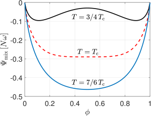
Figure 1: The free energy of mixing $\Psi_{\mathrm{mix}}$ vs. $\phi$ for various temperatures $T$.

4.2 Diffusive flux

Given the Helmholtz free energy $\Psi$, the components of the diffusive flux can be written as

$$\begin{array}[]{l}j_{\alpha}=-\displaystyle\frac{M}{J}\,\mu_{\mathrm{c},\alpha}\,,\end{array}$$ (36)

where $M=D\,\phi\,(1-\phi)$, with $D=$ const., is the degenerate mobility (Wells et al.,, 2006) and

$$\begin{array}[]{l}\mu_{\mathrm{c}}=\mu_{\mathrm{b}}+\mu_{\mathrm{i}}\,,\end{array}$$ (37)

is the chemical potential that has the bulk and interface contributions

$$\begin{array}[]{lll}\mu_{\mathrm{b}}\!\!\!&:=&\!\!\!\displaystyle\frac{\partial{\Psi}}{\partial{\phi}}\,,\\[8.53581pt] \mu_{\mathrm{i}}\!\!\!&:=&\!\!\!-J\,\displaystyle\bigg{(}\frac{1}{J}\frac{\partial{\Psi}}{\partial{\phi_{;\alpha}}}\bigg{)}_{\!\!;\alpha}\,,\end{array}$$ (38)

respectively (see Appendix A). Division by $J$ is included in (36) since $j_{\alpha}$ relates to the current area, while $\mu_{\mathrm{c}}$ is defined per reference area. From (27)-(35) we find

$$\begin{array}[]{lrl}\mu_{\mathrm{b}}\!\!\!&=&\!\!\!\mu_{\phi}+\mu_{\mathrm{el}}\,,\\ \mu_{\phi}\!\!\!&=&\!\!\!Nk_{\mathrm{B}}T\ln{\displaystyle\frac{\phi}{1-\phi}}+N\omega\,(1-2\phi)\,,\\[4.2679pt] \mu_{\mathrm{el}}\!\!\!&=&\!\!\!\Psi^{\prime}_{\mathrm{el}}\,,\\[4.2679pt] \mu_{\mathrm{i}}\!\!\!&=&\!\!\!-J\,N\,\omega\,\lambda\,\Delta_{\mathrm{s}}\phi\,,\end{array}$$ (39)

where $(...)^{\prime}:=\partial.../\partial\phi$. The elastic contribution to the chemical potential follows from (28) as

$$\begin{array}[]{l}\mu_{\mathrm{el}}=\displaystyle\frac{K^{\prime}}{4}\big{(}J^{2}-1-2\,\ln J\big{)}+\frac{G^{\prime}}{2}\big{(}I_{1}/J-2\big{)}+\frac{c^{\prime}}{2}\big{(}b_{\alpha\beta}-B_{\alpha\beta}\big{)}\big{(}b^{\alpha\beta}_{0}-B^{\alpha\beta}\big{)}~{}.\end{array}$$ (40)

The diffusive flux can be decomposed as

$$\begin{array}[]{l}j^{\alpha}=j^{\alpha}_{\phi}+j^{\alpha}_{\mathrm{el}}+j^{\alpha}_{\mathrm{i}}\,,\end{array}$$ (41)

with

$$\begin{array}[]{l}j^{\alpha}_{\bullet}=-\displaystyle\frac{M}{J}a^{\alpha\beta}\,\mu_{\bullet,\beta}\,,\end{array}$$ (42)

for the three different contributions.

4.3 Stress and moments

The components of the stress and moment tensors follow from the Helmholtz free energy per reference area as

$$\begin{array}[]{lll}\sigma^{\alpha\beta}\!\!\!&=&\!\!\!\displaystyle\frac{2}{J}\frac{\partial{\Psi}}{\partial{a_{\alpha\beta}}}-\eta\,\dot{a}^{\alpha\beta}\,,\\[11.38109pt] M^{\alpha\beta}\!\!\!&=&\!\!\!\displaystyle\frac{1}{J}\frac{\partial{\Psi}}{\partial{b_{\alpha\beta}}}\end{array}$$ (43)

(Sauer et al.,, 2017; Sahu et al.,, 2017). The second term in (43.1) accounts for viscous in-plane stress considering finite linear surface shear viscosity (Rangamani et al.,, 2013, 2014; Sahu et al.,, 2017). Here $\eta$ is the dynamic surface viscosity and $\dot{a}^{\alpha\beta}=-a^{\alpha\gamma}\,\dot{a}_{\gamma\delta}\,a^{\delta\beta}$ corresponds to the components of the surface velocity gradient multiplied by $-$2 (Sauer,, 2018). Given the different contributions to the total Helmholtz free energy in (27), the stress components follow as

$$\begin{array}[]{l}\sigma^{\alpha\beta}=\sigma^{\alpha\beta}_{\mathrm{el}}+\sigma^{\alpha\beta}_{\mathrm{visc}}+\sigma^{\alpha\beta}_{\mathrm{CH}}\,,\end{array}$$ (44)

where the elastic stress contribution is

$$\begin{array}[]{l}\sigma^{\alpha\beta}_{\mathrm{el}}:=\displaystyle\frac{2}{J}\frac{\partial{\Psi_{\mathrm{el}}}}{\partial{a_{\alpha\beta}}}=\displaystyle\frac{K(\phi)}{2J}\big{(}J^{2}-1\big{)}\,a^{\alpha\beta}+\frac{G(\phi)}{2J^{2}}\Big{(}2A^{\alpha\beta}-I_{1}\,a^{\alpha\beta}\Big{)}\,,\end{array}$$ (45)

the viscous stress contribution is

$$\begin{array}[]{l}\sigma^{\alpha\beta}_{\mathrm{visc}}:=-\displaystyle\eta(\phi)\,\dot{a}^{\alpha\beta}\,,\end{array}$$ (46)

and the Korteweg stresses (Sahu et al.,, 2017) due to the Cahn-Hilliard energy is given by

$$\begin{array}[]{l}\sigma^{\alpha\beta}_{\mathrm{CH}}:=\displaystyle\frac{2}{J}\frac{\partial{\Psi_{\mathrm{CH}}}}{\partial{a_{\alpha\beta}}}=N\,\omega\frac{\lambda}{2}\big{(}a^{\alpha\beta}\,a^{\gamma\delta}-2a^{\alpha\gamma}a^{\beta\delta}\big{)}\,\phi_{;\gamma}\,\phi_{;\delta}\,.\end{array}$$ (47)

These Korteweg stresses lead to a coupling between in-plane phase transformations and out-of-plane bending according to (25.2). We illustrate the Korteweg stresses in the numerical examples of Sec. 7.
The components of the moment tensor only stem from $\Psi_{\mathrm{bend}}$ in (28). They follow as

$$\begin{array}[]{l}M^{\alpha\beta}=\displaystyle\frac{c(\phi)}{J}\big{(}A^{\alpha\gamma}b_{\gamma\delta}A^{\beta\delta}-B^{\alpha\beta}\big{)}\,.\end{array}$$ (48)

We emphasize that $\sigma^{\alpha\beta}$ are the stresses following from constitution, but they are not the total stresses appearing in the equations of motion. These are

$$\begin{array}[]{l}N^{\alpha\beta}=\sigma^{\alpha\beta}+b^{\beta}_{\gamma}M^{\gamma\alpha}\,,\end{array}$$ (49)

as noted in Sec. 3.2.

4.4 Mixture rules

In this section, we propose a model for the dependency of the material parameters on the field variable $\phi\in[0,1]$. Recall that $\phi$ characterizes the current composition of the mixture and the two separate phases are characterized by values close to 0 and close to 1. Due to the characteristics of $\Psi_{\mathrm{mix}}$ shown in Fig. 1, $\phi$ does not attain the exact values of 0 and 1.

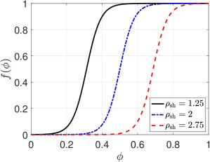
Figure 2: Modeling of mixtures: Characteristics of Eq. (51).

At any point $\boldsymbol{x}\in\mathcal{S}$ there will thus be a mixture of two phases. In this work, we model the behavior of the mixture by proposing the following mixture rule

$$\begin{array}[]{lll}K(\phi)\!\!\!&=&\!\!\!K_{1}\,f(\phi)+K_{0}\,(1-f(\phi))\,,\\[2.84526pt] G(\phi)\!\!\!&=&\!\!\!G_{1}\,f(\phi)+G_{0}\,(1-f(\phi))\,,\\[2.84526pt] c(\phi)\!\!\!&=&\!\!\!c_{1}\,f(\phi)+c_{0}\,(1-f(\phi))\,,\\[2.84526pt] \eta(\phi)\!\!\!&=&\!\!\!\eta_{1}\,f(\phi)+\eta_{0}\,(1-f(\phi))\,,\end{array}$$ (50)

with the interpolation function

$$\begin{array}[]{lll}f(\phi)=\displaystyle\frac{1}{2}\Big{(}1+\text{tanh}\left(-\rho_{\mathrm{sh}}\,\pi+4\,\pi\,\phi\right)\Big{)}\,.\end{array}$$ (51)

Here, $K_{i}$, $G_{i}$, $c_{i}$ and $\eta_{i}$ are the material parameters corresponding to $f(\phi)=i$, $i=0,1$. The constant $\rho_{\mathrm{sh}}\in\mathbb{R}$ prescribes whether a smaller or a larger portion of the phase interface is characterized by material properties corresponding to $\phi=1$. The function $f(\phi)$ is shown in Fig. 2 for different $\rho_{\mathrm{sh}}$. In the subsequent examples, $\rho_{\mathrm{sh}}=1.25$ is chosen in order to increase the influence of phase $\phi=1$, which is the softer phase in the examples.

5 Weak form

This section presents the weak form of PDEs (18) and (20). Combining (18) with (41), (42) and (39) and combining (25) with (24), (48) and (6), shows that both are fourth-order PDEs (Sahu et al.,, 2017). Hence, the surface divergence theorem is applied twice in order to obtain second-order weak forms.

5.1 Weak form for the Kirchhoff-Love thin shell equation

For Kirchhoff-Love shells the weak form is given by

$$\begin{array}[]{l}G_{\mathrm{in}}+G_{\mathrm{int}}-G_{\mathrm{ext}}=0\quad\forall\,\delta\boldsymbol{x}\in\mathcal{U}\,,\end{array}$$ (52)

with

$$\begin{array}[]{lll}G_{\mathrm{in}}\!\!\!&:=&\!\!\!\displaystyle\int_{\mathcal{S}}\delta\boldsymbol{x}\cdot\rho\,\dot{\boldsymbol{v}}\,\mathrm{d}a\,,\\[11.38109pt] G_{\mathrm{int}}\!\!\!&:=&\!\!\!\displaystyle\int_{\mathcal{S}}\frac{1}{2}\,\delta a_{\alpha\beta}\,\sigma^{\alpha\beta}\,\mathrm{d}a+\int_{\mathcal{S}}\delta b_{\alpha\beta}\,M^{\alpha\beta}\,\mathrm{d}a\,,\\[11.38109pt] G_{\mathrm{ext}}\!\!\!&:=&\!\!\!\displaystyle\int_{\mathcal{S}}\delta\boldsymbol{x}\cdot\boldsymbol{f}\,\mathrm{d}a+\int_{\partial_{t}\mathcal{S}}\delta\boldsymbol{x}\cdot\boldsymbol{T}\,\mathrm{d}s+\int_{\partial_{m}\mathcal{S}}\delta\boldsymbol{n}\cdot\boldsymbol{M}\,\mathrm{d}s\end{array}$$ (53)

(Sauer and Duong,, 2017). Here, $\mathcal{U}=\left\{\delta\boldsymbol{x}\in\mathcal{H}^{2}\big{(}\mathcal{S}(\boldsymbol{x},t)^{3}\big{)}|\,\delta\boldsymbol{x}=0\,\text{on}\,\partial_{x}\mathcal{S}\,,\,\delta\boldsymbol{n}=0\,\text{on}\,\partial_{n}\mathcal{S}\right\}$ is the space of suitable surface variations, where $\mathcal{H}^{2}$ is the Sobolev space with square integrable first and second derivatives and $\partial_{x}\mathcal{S}$ and $\partial_{n}\mathcal{S}$ are the Dirichlet boundaries for displacements and rotations. Further, $\boldsymbol{f}=f^{\alpha}\,\boldsymbol{a}_{\alpha}+p\,\boldsymbol{n}$, $\boldsymbol{T}=\mbox{\boldmath$\sigma$}^{\mathrm{T}}\mbox{\boldmath$\nu$}$ and $\boldsymbol{M}=\mbox{\boldmath$\mu$}^{\mathrm{T}}\mbox{\boldmath$\nu$}$ denote prescribed surface forces, edge tractions and edge moments. The latter act on the boundaries $\partial_{t}\mathcal{S}$ and $\partial_{m}\mathcal{S}$, respectively. For closed surfaces (as used in the examples of Sec. 7), $\partial_{t}\mathcal{S}=\partial_{m}\mathcal{S}=\emptyset$. If desired, $\mathrm{d}a=J\,\mathrm{d}A$ can be used to map integrals to the reference surface $\mathcal{S}_{0}$.

5.2 Weak form for the Cahn-Hilliard surface equation

Multiplying field equation (18) with the test function $\delta\phi$, and applying the surface divergence theorem

$$\begin{array}[]{l}\displaystyle\int_{\mathcal{S}}j^{\alpha}_{;\alpha}\,\mathrm{d}a=\displaystyle\int_{\partial\mathcal{S}}j^{\alpha}\,\nu_{\alpha}\,\mathrm{d}s\,,\end{array}$$ (54)

gives

$$\begin{array}[]{l}\displaystyle\int_{\mathcal{S}}\delta\phi\,\rho\,\dot{\phi}\,\mathrm{d}a-\int_{\mathcal{S}}\delta\phi_{;\alpha}\,j^{\alpha}\,\mathrm{d}a+\int_{\partial_{j}\mathcal{S}}\delta\phi\,\bar{\boldsymbol{j}}\cdot\mbox{\boldmath$\nu$}\,\mathrm{d}s=0\quad\forall\,\delta\phi\in\mathcal{V}\,,\end{array}$$ (55)

where $\bar{\boldsymbol{j}}$ is the prescribed flux on boundary $\partial_{j}\mathcal{S}$ with outward unit normal $\mbox{\boldmath$\nu$}=\nu_{\alpha}\boldsymbol{a}^{\alpha}$. Here we have assumed that $\delta\phi=0$ on $\partial\mathcal{S}\backslash\partial_{j}\mathcal{S}$. Further, $\mathcal{V}=\left\{\delta\phi\in\mathcal{H}^{2}\big{(}\mathcal{S}(\phi,t)\big{)}\right|\,\delta\phi=0\,\text{on}\,\partial\mathcal{S}\backslash\partial_{j}\mathcal{S}\}$ is the space of suitable test functions.
According to (41) and (42) the flux $j^{\alpha}$ has three contributions. The last of those, the interfacial flux $j^{\alpha}_{\mathrm{i}}$, contains three derivatives, and so we again apply the surface divergence theorem to this term to reduce it to second order. In order to avoid handling complex expressions for terms arising from $\nabla_{\!\!\mathrm{s}}\mu_{\mathrm{el}}$ that later need to be linearized, we will apply the surface divergence theorem also to $j^{\alpha}_{\mathrm{el}}$. Doing so, we obtain,

$$\begin{array}[]{l}\displaystyle\int_{\mathcal{S}}\delta\phi_{;\alpha}\,(j^{\alpha}_{\mathrm{i}}+j^{\alpha}_{\mathrm{el}})\,\mathrm{d}a=\int_{\mathcal{S}_{0}}\big{(}\nabla_{\!\!\mathrm{s}}\delta\phi\cdot\nabla_{\!\!\mathrm{s}}M+\Delta_{\mathrm{s}}\delta\phi\,M\big{)}\big{(}\mu_{\mathrm{i}}+\mu_{\mathrm{el}}\big{)}\,\mathrm{d}A+\int_{\partial_{r}\mathcal{S}}\nabla_{\!\!\mathrm{s}}\delta\phi\cdot\mbox{\boldmath$\nu$}\,\bar{r}\,\mathrm{d}s\,,\end{array}$$ (56)

where $\bar{r}$ is the prescribed boundary value for the quantity $r:=M(\lambda\,\omega N\Delta_{\mathrm{s}}\phi-\mu_{\mathrm{el}}/J)$. Here we have assumed that $\nabla_{\!\!\mathrm{s}}\delta\phi=\mathbf{0}$ on $\partial\mathcal{S}\backslash\partial_{r}\mathcal{S}$, and transformed integrals using $\mathrm{d}a=J\,\mathrm{d}A$. Writing $\nabla_{\!\!\mathrm{s}}M=M^{\prime}\,\nabla_{\!\!\mathrm{s}}\phi$ and $\delta\phi_{;\alpha}\,j^{\alpha}_{\phi}=-\nabla_{\!\!\mathrm{s}}\delta\phi\cdot\nabla_{\!\!\mathrm{s}}\phi\,M\mu^{\prime}_{\phi}/J$ then leads to the weak form

$$\begin{array}[]{l}\bar{G}_{\mathrm{in}}+\bar{G}_{\mathrm{int}}-\bar{G}_{\mathrm{ext}}=0\quad\forall\,\delta\phi\in\mathcal{V}\,,\end{array}$$ (57)

with

$$\begin{array}[]{lll}\bar{G}_{\mathrm{in}}\!\!\!&:=&\!\!\!\displaystyle\int_{\mathcal{S}}\delta\phi\,\rho\,\dot{\phi}\,\mathrm{d}a\,,\\[11.38109pt] \bar{G}_{\mathrm{int}}\!\!\!&:=&\!\!\!\displaystyle\int_{\mathcal{S}_{0}}\nabla_{\!\!\mathrm{s}}\delta\phi\cdot\Big{(}M\mu^{\prime}_{\phi}-M^{\prime}\big{(}\mu_{\mathrm{i}}+\mu_{\mathrm{el}}\big{)}\Big{)}\,\nabla_{\!\!\mathrm{s}}\phi\,\mathrm{d}A-\int_{\mathcal{S}_{0}}\Delta_{\mathrm{s}}\delta\phi\,M\big{(}\mu_{\mathrm{i}}+\mu_{\mathrm{el}}\big{)}\,\mathrm{d}A\,,\\[11.38109pt] \bar{G}_{\mathrm{ext}}\!\!\!&:=&\!\!\!-\displaystyle\int_{\partial_{j}\mathcal{S}}\delta\phi\,\bar{\boldsymbol{j}}\cdot\mbox{\boldmath$\nu$}\,\mathrm{d}s+\int_{\partial_{r}\mathcal{S}}\nabla_{\!\!\mathrm{s}}\delta\phi\cdot\mbox{\boldmath$\nu$}\,\bar{r}\,\mathrm{d}s\,.\end{array}$$ (58)

For closed surfaces (as in the examples of Sec. 7), $\partial_{j}\mathcal{S}=\partial_{r}\mathcal{S}=\emptyset$ and hence $\bar{G}_{\mathrm{ext}}=0$.

Remark: As an alternative to using the surface divergence theorem on $\nabla_{\!\!\mathrm{s}}\mu_{\mathrm{el}}$, this term can be expanded as in footnote 7. This results in

$$\begin{array}[]{l}\bar{G}_{\mathrm{int}}:=\displaystyle\int_{\mathcal{S}_{0}}\nabla_{\!\!\mathrm{s}}\delta\phi\cdot\bigg{[}\Big{(}M\big{(}\mu^{\prime}_{\phi}+\mu^{\prime}_{\mathrm{el}}\big{)}-M^{\prime}\mu_{\mathrm{i}}\Big{)}\,\nabla_{\!\!\mathrm{s}}\phi+M\frac{\partial{\mu_{\mathrm{el}}}}{\partial{b_{\alpha\beta}}}b_{\alpha\beta;\gamma}\,\boldsymbol{a}^{\gamma}\bigg{]}\,\mathrm{d}A-\int_{\mathcal{S}_{0}}\Delta_{\mathrm{s}}\delta\phi\,M\mu_{\mathrm{i}}\,\mathrm{d}A\,.\end{array}$$ (59)

This avoids having $\mu_{\mathrm{el}}$ inside $\bar{r}$, but it requires dealing with $\partial\mu_{\mathrm{el}}/\partial b_{\alpha\beta}\,b_{\alpha\beta;\gamma}\,\boldsymbol{a}^{\gamma}$ in the discretization and linearization of the coupled system. Therefore we will use (58) instead of (59).

5.3 Dimensionless form

The preceding equations can be normalized by defining dimensionless quantities for position, time and the Helmholtz free energy as

$$\begin{array}[]{l}\boldsymbol{x}^{\star}:=\displaystyle\frac{\boldsymbol{x}}{L_{0}}\,,\quad t^{\star}:=\displaystyle\frac{t}{T_{0}}\,,\quad\Psi^{\star}:=\displaystyle\frac{\Psi}{\Psi_{0}}\,,\end{array}$$ (60)

where $L_{0}$, $T_{0}$ and $\Psi_{0}$ are chosen scales for length, time and energy density, respectively. From this, the normalization of surface stress, surface moment, chemical potential, mobility, density and mass flux follow as

$$\begin{array}[]{l}\sigma^{\alpha\beta}_{\star}:=\displaystyle\frac{\sigma^{\alpha\beta}}{\Psi_{0}}\,,\quad M^{\alpha\beta}_{\star}:=\displaystyle\frac{M^{\alpha\beta}}{\Psi_{0}L_{0}}\,,\quad\mu_{\mathrm{c}}^{\star}:=\displaystyle\frac{\mu_{\mathrm{c}}}{\Psi_{0}}\,,\quad M^{\star}:=\displaystyle\frac{M}{T_{0}}\,,\quad\rho^{\star}:=\displaystyle\frac{\rho}{\rho_{0}}\,,\quad j^{\alpha}_{\star}:=\displaystyle\frac{j^{\alpha}}{j_{0}}\,,\end{array}$$ (61)

where $\rho_{0}:=T_{0}^{2}\Psi_{0}/L_{0}^{2}$ and $j_{0}:=\rho_{0}/T_{0}$. Further, the normalizations of the temporal and spatial derivative operators yield

$$\begin{array}[]{l}\displaystyle\frac{\partial{...}}{\partial{t^{\star}}}:=T_{0}\frac{\partial{...}}{\partial{t}}\,,\quad\nabla_{\!\!\mathrm{s}}^{\star}:=L_{0}\nabla_{\!\!\mathrm{s}}\,,\quad\Delta_{\mathrm{s}}^{\star}:=L_{0}^{2}\Delta_{\mathrm{s}}\,.\end{array}$$ (62)

With these definitions, the weak forms in Eq. (52) and (57) can be fully normalized as

$$\begin{array}[]{l}G^{\star}:=\displaystyle\frac{G}{\Psi_{0}L_{0}^{2}}\,,\quad\bar{G}^{\star}:=\displaystyle\frac{\bar{G}}{\Psi_{0}T_{0}}\,.\end{array}$$ (63)

Likewise,

$$\begin{array}[]{l}\bar{\Psi}^{\star}:=\displaystyle\frac{\bar{\Psi}}{\Psi_{0}L_{0}^{2}}\,,\quad\bar{\Psi}:=\displaystyle\int_{\mathcal{S}_{0}}\Psi\,\mathrm{d}A\end{array}$$ (64)

is the normalization of the total energy in the system. In the following, we will only work with the dimensionless form of all equations and will omit the superscript $\star$ for notational simplicity. In the examples we use $N\omega=\Psi_{0}$ and $Nk_{\mathrm{B}}T=\Psi_{0}/3$.

6 Discretization of the coupled system

This section presents the discretization of the governing equations in the framework of isogeometric finite elements. Due to the smoothness of spline basis functions, we can directly discretize the fields within the two second-order weak forms that describe the coupled problem. That is, we do not need to employ rotational degrees-of-freedom (dofs) or resort to mixed formulations. The spatial discretization used here is based on the unstructured spline construction presented in Sec. 6.1, which is at least $C^{1}$-continuous at all points $\boldsymbol{x}(t)$ for all $t$. This is then used in Secs. 6.2 and 6.3 to discretize the two governing weak forms. In Sec. 6.4 we discuss their temporal discretization using an adaptive time-stepping scheme.

6.1 Unstructured spline spaces

The numerical examples presented in this work utilize structured NURBS meshes and unstructured quadrilateral meshes to describe the surface geometry. The construction of unstructured spline spaces for the latter is based on the approach of Toshniwal et al., 2017b . This approach is advantageous since it allows the description of surfaces that are point-wise $C^{1}$-continuous even during deformation. The approach is briefly summarized here.

The tasks of geometric modeling and computational analysis place differing requirements on the spaces of spline functions to be used. Acknowledging these differences, Toshniwal et al., 2017b built separate spline spaces for these tasks, $\mathbb{S}_{D}$ and $\mathbb{S}_{A}$, respectively. The following sections give a conceptual overview of the construction and properties of the spline basis functions spanning $\mathbb{S}_{D}$ and $\mathbb{S}_{A}$.

6.1.1 Construction of spline spaces

The construction of spline spaces is explained using the concept of extraction operators (Borden et al.,, 2011). Those allow to write the IGA formulation in classical FE notation. We explain this concept with piecewise-polynomial (abbreviated as p-w-p) splines in mind (B-/T-/LR-/HBS-splines, for instance). The p-w-p splines restricted to any parametric element of the mesh $\Omega_{e}$ are tensor-product polynomials. Then, the extraction operator is the map from the local tensor-product polynomial basis, typically chosen as the Bernstein polynomial basis, to the element-local polynomial representation of the spline basis.

Keeping the above basics in mind, the constructions of splines reduces to defining suitable extraction operators for each element. We do this for the basis functions spanning $\mathbb{S}_{D}$ and $\mathbb{S}_{A}$, $N^{D}_{i}$ and $N^{A}_{i}$, respectively, in the following manner:

1. Initial, macro extractions: First, the p-w-p forms of $N^{D}_{i}$ and $N^{A}_{i}$ on the underlying quadrilateral mesh are initialized. This amounts to initialization of the extraction operators for these splines on each element; see Appendix B for details.

2. Smoothed, micro extraction: After initialization, $N^{D}_{i}$ and $N^{A}_{i}$ are only $C^{0}$-smooth on the elements containing extraordinary points (EPs), i.e., vertices where the number of edges that meet is not equal to $4$, like the central vertex in Fig. 3 left. Then, the splines are smoothed by (a) splitting their p-w-p forms on the elements containing EPs (Nguyen and Peters,, 2016) using the de Casteljau algorithm (Piegl and Tiller,, 2012), and then (b) by a smoothing of the p-w-p forms using a smoothing matrix and the theory of D-patches (Reif,, 1997).

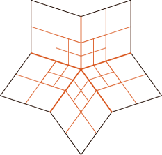
Figure 3: The above figures show a neighborhood of an extraordinary point. The left side displays the 2-ring elements that surround the extraordinary point, while the middle shows the local dof structure around the extraordinary point for $\mathbb{S}_{A}$. Instead of all mesh vertices being identified as dofs, some mesh vertices are labelled inactive (red disk), and in their place dofs on the adjacent faces are introduced (blue squares); then, the face-based dofs and the mesh vertices not labelled inactive collectively form the full set of active dofs (black disks and blue squares) – the ones used for performing computations. Each dof is associated to a $C^{k}$ smooth spline function, $k\geq 1$. The rightmost figure elucidates the smoothness of an arbitrary spline in the space spanned by these functions – smoothness across the red (resp. black) edges is $C^{1}$ (resp. $C^{2}$), while it is $C^{\infty}$ in the white space as the splines are simply polynomials in the element interiors.

One of the salient features of the above construction is that each step is carried out while ensuring satisfaction of isogeometric compatibility, $\mathbb{S}_{D}\subset\mathbb{S}_{A}$. This is a sufficient condition for allowing exact representation of geometries built using $\mathbb{S}_{D}$ as members of $\mathbb{S}_{A}$. In other words, at each step of the construction, we ensure that the following holds,

$$\begin{bmatrix}N^{D}_{1}\\ \vdots\\ N^{D}_{n_{D}}\end{bmatrix}=\mathbf{C}^{A\rightarrow D}\begin{bmatrix}N^{A}_{1}\\ \vdots\\ N^{A}_{n_{A}}\end{bmatrix},$$ (65)

where $\mathbf{C}^{A\rightarrow D}$ is an explicitly computable matrix, and $n_{A}$ and $n_{D}$ are the numbers of control points (or nodes) used for the analysis and design, respectively. Then, isogeometric compatibility follows trivially,

$$\mathbb{S}_{D}:=\text{span}(N^{D}_{1},\dots,N^{D}_{n_{D}})\subset\text{span}(N^{A}_{1},\dots,N^{A}_{n_{A}})=:\mathbb{S}_{A}\,.$$ (66)

Initial geometries at time $t=0$, $\mathcal{S}(0)$, are built using $\mathbb{S}_{D}$ and, because of isogeometric compatibility, we can express them exactly as members of $\mathbb{S}_{A}$. In the subsequent analysis only $\mathbb{S}_{A}$ is needed. Therefore, we restrict the remaining discussion to the usage of $\mathbb{S}_{A}$ and omit index $A$ to simplify notation, i.e.

$$N_{i}:=N^{A}_{i}\,,\qquad\mathbb{S}:=\mathbb{S}_{A}\,.$$ (67)

The dof structure corresponding to $\mathbb{S}$ in the vicinity of extraordinary points is shown in the middle of Fig. 3. The smoothness of an arbitrary spline $s\in\mathbb{S}$ is illustrated on the right of Fig. 3. As shown, the extraordinary point’s neighborhood contains edges across which the smoothness is only $C^{1}$ (depicted in red in the figure). Also note that this zone of $C^{1}$-continuity is limited to the 2-ring elements of each extraordinary point (at the coarsest level of refinement), and outside of this zone the splines are maximally smooth, i.e., $C^{2}$-continuous.

6.1.2 Properties of $\mathbb{S}$

The spline space $\mathbb{S}$ is built exclusively from bi-cubic polynomial pieces, and is identical to the space of bi-cubic analysis-suitable T-splines (or, AST-splines) (Scott et al.,, 2013; Li,, 2015) in the regular (locally structured) regions of the mesh. In particular, the basis functions spanning $\mathbb{S}$ form a convex partition of unity and are locally supported. Additionally, the space $\mathbb{S}$ was observed to possess good approximation properties as evidenced by the suite of numerical tests presented in Toshniwal et al., 2017b , and makes numerical investigation of high-order problems on arbitrary surfaces possible.

6.1.3 Spatial discretization of primary fields

In this section, finite dimensional approximations to all primary fields of interest (surface geometry and phase field order parameter) will be expressed as members of $\mathbb{S}$. Let $n_{e}$ spline basis functions, with global indices $i_{1},\dots,i_{n_{e}}$, be supported on parametric element $\Omega_{e}$. Then, we can express the local element representations of the surface $\mathcal{S}$, $\mathcal{S}_{0}$ and phase field $\phi$ as,

$$\begin{array}[]{l}\boldsymbol{x}^{h}=\mathbf{N}\,\mathbf{x}_{e}\,,\qquad\boldsymbol{X}^{h}=\mathbf{N}\,\mathbf{X}_{e}\,,\end{array}$$ (68)

and,

$$\begin{array}[]{l}\phi^{h}=\bar{\mathbf{N}}\,\mbox{\boldmath$\phi$}_{e}\,,\end{array}$$ (69)

respectively, where,

$$\begin{array}[]{l}\mathbf{N}:=[N_{i_{1}}\mathbf{1},\,N_{i_{2}}\mathbf{1},\,...,\,N_{i_{n_{e}}}\mathbf{1}]\,,\end{array}$$ (70)

$$\begin{array}[]{l}\bar{\mathbf{N}}:=[N_{i_{1}},\,N_{i_{2}},\,...,\,N_{i_{n_{e}}}]\,.\end{array}$$ (71)

Here, $\mathbf{1}$ denotes the $(3\times 3)$ identity matrix, and $\mathbf{X}_{e}$, $\mathbf{x}_{e}$ and $\mbox{\boldmath$\phi$}_{e}$ denote element-level vectors containing the positions and dofs at nodes $i_{1},\dots,i_{n_{e}}$. These local vectors can be extracted from the global vectors $\mathbf{X}$, $\mathbf{x}$ and $\phi$ that contain all nodal positions and dofs. The respective variations are defined analogously, given by

$$\begin{array}[]{l}\delta\boldsymbol{x}^{h}=\mathbf{N}\,\delta\mathbf{x}_{e}\,,\qquad\delta\boldsymbol{X}^{h}=\mathbf{N}\,\delta\mathbf{X}_{e}\,,\end{array}$$ (72)

and,

$$\begin{array}[]{l}\delta\phi^{h}=\bar{\mathbf{N}}\,\delta\mbox{\boldmath$\phi$}_{e}\,.\end{array}$$ (73)

Using the above equations, the weak forms for the surface deformation and the phase field are discretized as described in Secs. 6.2 and 6.3, respectively.

6.2 Spatial discretization of the mechanical weak form

Using Eqs. (68) and (69), the tangent vectors on the surface are discretized as

$$\begin{array}[]{lll}\boldsymbol{a}_{\alpha}^{h}\!\!\!&=&\!\!\!\mathbf{N}_{\!,\alpha}\,\mathbf{x}_{e}\,,~{}\mathrm{and}\quad\boldsymbol{A}_{\alpha}^{h}=\mathbf{N}_{\!,\alpha}\,\mathbf{X}_{e}\,,\end{array}$$ (74)

where $\mathbf{N}_{\!,\alpha}:=\partial\mathbf{N}/\partial\xi^{\alpha}$. The discretized tangent vectors of (74) lead to the discretized normal vectors $\boldsymbol{n}^{h}$ and $\boldsymbol{N}^{h}$ following Eq. (4). The metric tensor and curvature components can then be expressed as

$$\begin{array}[]{lll}a_{\alpha\beta}^{h}\!\!\!&=&\!\!\!\mathbf{x}_{e}^{\mathrm{T}}\mathbf{N}^{\mathrm{T}}_{\!,\alpha}\,\mathbf{N}_{\!,\beta}\,\mathbf{x}_{e}\,,~{}\mathrm{and}\quad b_{\alpha\beta}^{h}=\boldsymbol{n}^{h}\cdot\mathbf{N}_{\!,\alpha\beta}\,\mathbf{x}_{e}\,,\end{array}$$ (75)

and similarly

$$\begin{array}[]{lll}A_{\alpha\beta}^{h}\!\!\!&=&\!\!\!\mathbf{X}_{e}^{\mathrm{T}}\mathbf{N}^{\mathrm{T}}_{\!,\alpha}\,\mathbf{N}_{\!,\beta}\,\mathbf{X}_{e}\,,~{}\mathrm{and}\quad B_{\alpha\beta}^{h}=\boldsymbol{N}^{h}\cdot\mathbf{N}_{\!,\alpha\beta}\,\mathbf{X}_{e}\,.\end{array}$$ (76)

The contravariant metrics $[a^{\alpha\beta}_{h}]=[a_{\alpha\beta}^{h}]^{-1}$ and $[A^{\alpha\beta}_{h}]=[A_{\alpha\beta}^{h}]^{-1}$ then follow. Using Eq. (72), the variations of the surface metric and curvature can be obtained as

$$\begin{array}[]{lll}\delta a_{\alpha\beta}^{h}\!\!\!&=&\!\!\!\delta\mathbf{x}_{e}^{\mathrm{T}}\big{(}\mathbf{N}^{\mathrm{T}}_{\!,\alpha}\,\mathbf{N}_{\!,\beta}+\mathbf{N}^{\mathrm{T}}_{\!,\beta}\,\mathbf{N}_{\!,\alpha}\big{)}\,\mathbf{x}_{e}\,,~{}\mathrm{and}\quad\delta b_{\alpha\beta}^{h}=\delta\mathbf{x}_{e}^{\mathrm{T}}\,\mathbf{N}^{\mathrm{T}}_{\!;\alpha\beta}\,\boldsymbol{n}^{h}\,,\end{array}$$ (77)

with

$$\begin{array}[]{l}\mathbf{N}_{\!;\alpha\beta}:=\mathbf{N}_{\!,\alpha\beta}-\Gamma^{\gamma}_{\alpha\beta}\,\mathbf{N}_{\!,\gamma}\,.\end{array}$$ (78)

Here,

$$\begin{array}[]{l}\Gamma^{\gamma}_{\alpha\beta}=\mathbf{x}_{e}^{\mathrm{T}}\,\mathbf{N}^{\mathrm{T}}_{,\alpha\beta}\,a^{\gamma\delta}_{h}\,\mathbf{N}_{,\delta}\,\mathbf{x}_{e}\end{array}$$ (79)

denotes the discretized Christoffel symbols. Using the above expressions, the discretized mechanical weak form becomes

$$\begin{array}[]{l}\delta\mathbf{x}^{\mathrm{T}}\,\big{[}\mathbf{f}_{\mathrm{in}}+\mathbf{f}_{\mathrm{int}}-\mathbf{f}_{\mathrm{ext}}\big{]}=0\quad\forall~{}\delta\mathbf{x}\in\mathcal{U}^{h}\,,\end{array}$$ (80)

where the global force vectors $\mathbf{f}_{\mathrm{in}}$, $\mathbf{f}_{\mathrm{int}}$ and $\mathbf{f}_{\mathrm{ext}}$ are assembled from their respective elemental contributions

$$\begin{array}[]{lll}\mathbf{f}^{e}_{\mathrm{in}}\!\!\!&:=&\!\!\!\mathbf{m}_{e}\,\ddot{\mathbf{x}}_{e}~{},\quad\mathbf{m}_{e}:=\displaystyle\int_{\Omega^{e}}\rho\,\mathbf{N}^{\mathrm{T}}\mathbf{N}\,\mathrm{d}a\,,\\[11.38109pt] \mathbf{f}^{e}_{\mathrm{int}}\!\!\!&:=&\!\!\!\displaystyle\int_{\Omega^{e}}\sigma^{\alpha\beta}\,\mathbf{N}_{\!,\alpha}^{\mathrm{T}}\,\boldsymbol{a}^{h}_{\beta}\,\mathrm{d}a+\int_{\Omega^{e}}M^{\alpha\beta}\,\mathbf{N}^{\mathrm{T}}_{\!;\alpha\beta}\,\boldsymbol{n}^{h}\,\mathrm{d}a\,,\\[11.38109pt] \mathbf{f}^{e}_{\mathrm{ext}}\!\!\!&:=&\!\!\!\displaystyle\int_{\Omega^{e}}\mathbf{N}^{\mathrm{T}}\,p\,\boldsymbol{n}^{h}\,\mathrm{d}a+\displaystyle\int_{\Omega^{e}}\mathbf{N}^{\mathrm{T}}\,f^{\alpha}\,\boldsymbol{a}^{h}_{\alpha}\,\mathrm{d}a\,.\end{array}$$ (81)

Further, $\delta\mathbf{x}$ denotes the global vector of all nodal variations, and $\mathcal{U}^{h}:=\mathcal{U}\,\cap\,\mathbb{S}$ is its corresponding discrete space. The expression of $\mathbf{f}^{e}_{\mathrm{ext}}$, corresponds to the case that there are no boundary loads $\boldsymbol{T}$ and $\boldsymbol{M}$ acting on $\partial\mathcal{S}$. This is the case in all the subsequent examples. The extension to boundary loads can be found in Duong et al., (2017). $\mathbf{f}_{\mathrm{in}}$, $\mathbf{f}_{\mathrm{int}}$ and $\mathbf{f}_{\mathrm{ext}}$ depend on $\mathbf{x}(t)$, while $\mathbf{f}_{\mathrm{int}}$ also depends on $\mbox{\boldmath$\phi$}(t)$ through the material properties in $\sigma^{\alpha\beta}$ and $M^{\alpha\beta}$, and the Korteweg stresses $\sigma_{\mathrm{CH}}^{\alpha\beta}$. The resulting equations at the free nodes (after application of Dirichlet boundary conditions) can thus be written as

$$\begin{array}[]{l}\mathbf{f}(\mathbf{x},\mbox{\boldmath$\phi$})=\mathbf{M}\,\ddot{\mathbf{x}}+\mathbf{f}_{\mathrm{int}}(\mathbf{x},\mbox{\boldmath$\phi$})-\mathbf{f}_{\mathrm{ext}}(\mathbf{x})=\mathbf{0}~{},\end{array}$$ (82)

where $\mathbf{M}$ denotes the global mass matrix assembled from $\mathbf{m}_{e}$, and $\mathbf{x}$ and $\phi$ denote the global vectors of the unknown nodal positions and unknown nodal phase parameters.

6.3 Spatial discretization of the phase field equations

Using Eq. (8) and Eq. (69), we can write

$$\begin{array}[]{lll}\phi^{h}_{;\alpha}\!\!\!&=&\!\!\!\bar{\mathbf{N}}_{\!,\alpha}\,\mbox{\boldmath$\phi$}_{e}\,,\\[2.84526pt] \nabla_{\!\!\mathrm{s}}\phi^{h}\!\!\!&=&\!\!\!\boldsymbol{a}^{\alpha}_{h}\,\bar{\mathbf{N}}_{\!,\alpha}\,\mbox{\boldmath$\phi$}_{e}\,,\\[2.84526pt] \nabla_{\!\!\mathrm{s}}\delta\phi^{h}\!\!\!&=&\!\!\!\boldsymbol{a}^{\alpha}_{h}\,\bar{\mathbf{N}}_{\!,\alpha}\,\delta\mbox{\boldmath$\phi$}_{e}\,,\\[2.84526pt] \Delta_{\mathrm{s}}\phi^{h}\!\!\!&=&\!\!\!\Delta_{\mathrm{s}}\bar{\mathbf{N}}\,\mbox{\boldmath$\phi$}_{e}\,,\\[2.84526pt] \Delta_{\mathrm{s}}\delta\phi^{h}\!\!\!&=&\!\!\!\Delta_{\mathrm{s}}\bar{\mathbf{N}}\,\delta\mbox{\boldmath$\phi$}_{e}\,,\end{array}$$ (83)

where $\bar{\mathbf{N}}_{\!,\alpha}:=\partial\bar{\mathbf{N}}/\partial\xi^{\alpha}$ and

$$\begin{array}[]{l}\Delta_{\mathrm{s}}\bar{\mathbf{N}}:=a^{\alpha\beta}_{h}\,\bar{\mathbf{N}}_{\!;\alpha\beta}\,,\end{array}$$ (84)

with

$$\begin{array}[]{l}\bar{\mathbf{N}}_{\!;\alpha\beta}=\bar{\mathbf{N}}_{\!,\alpha\beta}-\Gamma^{\gamma}_{\alpha\beta}\,\bar{\mathbf{N}}_{\!,\gamma}\end{array}$$ (85)

according to Eq. (9). Here, $\boldsymbol{a}^{\alpha}_{h}=a^{\alpha\beta}_{h}\,\boldsymbol{a}^{h}_{\beta}$ and $\Gamma^{\gamma}_{\alpha\beta}$ follows from the surface discretization discussed in Sec. 6.2. The discretized weak form of the Cahn-Hilliard Eq. (57) then becomes

$$\begin{array}[]{l}\delta\mbox{\boldmath$\phi$}^{\mathrm{T}}\,\big{[}\bar{\mathbf{f}}_{\mathrm{in}}+\bar{\mathbf{f}}_{\mathrm{int}}-\bar{\mathbf{f}}_{\mathrm{ext}}\big{]}=0\quad\forall~{}\delta\mbox{\boldmath$\phi$}\in\mathcal{V}^{h}\,,\end{array}$$ (86)

where the global vectors $\bar{\mathbf{f}}_{\mathrm{in}}$, $\bar{\mathbf{f}}_{\mathrm{int}}$ and $\bar{\mathbf{f}}_{\mathrm{ext}}$ are assembled from their respective elemental contributions

$$\begin{array}[]{lll}\bar{\mathbf{f}}^{e}_{\mathrm{in}}\!\!\!&:=&\!\!\!\bar{\mathbf{m}}_{e}\,\dot{}\mbox{\boldmath$\phi$}_{e}\,,\quad\bar{\mathbf{m}}_{e}:=\displaystyle\int_{\Omega^{e}}\rho\,\bar{\mathbf{N}}^{\mathrm{T}}\bar{\mathbf{N}}\,\mathrm{d}a\,,\\[11.38109pt] \bar{\mathbf{f}}^{e}_{\mathrm{int}}\!\!\!&:=&\!\!\!\bar{\mathbf{k}}_{e}\,\mbox{\boldmath$\phi$}_{e}-\bar{\mathbf{f}}^{e}_{\mathrm{el}}\,,\quad\!\bar{\mathbf{k}}_{e}:=\!\displaystyle\int_{\Omega^{e}_{0}}\!\Big{[}\bar{\mathbf{N}}_{\!,\alpha}^{\mathrm{T}}\,a^{\alpha\beta}_{h}\Big{(}\!M\mu^{\prime}_{\phi}-M^{\prime}\big{(}\mu_{\mathrm{i}}+\mu_{\mathrm{el}}\big{)}\!\Big{)}\,\bar{\mathbf{N}}_{\!,\beta}+\Delta_{\mathrm{s}}\bar{\mathbf{N}}^{\mathrm{T}}J\lambda M\,\Delta_{\mathrm{s}}\bar{\mathbf{N}}\Big{]}\,\mathrm{d}A\,,\\[8.53581pt] \bar{\mathbf{f}}^{e}_{\mathrm{el}}\!\!\!&:=&\!\!\!\displaystyle\int_{\Omega^{e}_{0}}\Delta_{\mathrm{s}}\bar{\mathbf{N}}^{\mathrm{T}}M\mu_{\mathrm{el}}\,\mathrm{d}A\,,\\[11.38109pt] \bar{\mathbf{f}}^{e}_{\mathrm{ext}}\!\!\!&:=&\!\!\!-\displaystyle\int_{\Gamma_{j}^{e}}\bar{\mathbf{N}}^{\mathrm{T}}\,\bar{\boldsymbol{j}}\cdot\mbox{\boldmath$\nu$}\,\mathrm{d}s+\int_{\Gamma_{r}^{e}}\bar{\mathbf{N}}_{\!,\alpha}^{\mathrm{T}}\,\nu^{\alpha}\,\bar{r}\,\mathrm{d}s\,.\end{array}$$ (87)

Further, $\delta\mbox{\boldmath$\phi$}$ denotes the variation of global vector $\phi$, and $\mathcal{V}^{h}:=\mathcal{V}\,\cap\,\mathbb{S}$ is its corresponding discrete space. Note that the expressions in (87) depend on $\mbox{\boldmath$\phi$}_{e}$ through $M$, $\mu_{\phi}$, $\mu_{\mathrm{i}}$ and $\mu_{\mathrm{el}}$. They further depend on the geometry $\mathbf{x}_{e}$ through $a^{\alpha\beta}_{h}$, $\mu_{\mathrm{i}}$, $\mu_{\mathrm{el}}$, $\Delta_{\mathrm{s}}\bar{\mathbf{N}}$, $J$ and the boundary quantities $\nu$ and $\mathrm{d}s$. The resulting dynamical equations at the free nodes (after application of Dirichlet boundary conditions) can thus be written as

$$\begin{array}[]{l}\bar{\mathbf{f}}(\mathbf{x},\mbox{\boldmath$\phi$})=\bar{\mathbf{M}}\,\dot{}\mbox{\boldmath$\phi$}+\bar{\mathbf{f}}_{\mathrm{int}}(\mathbf{x},\mbox{\boldmath$\phi$})-\bar{\mathbf{f}}_{\mathrm{ext}}(\mathbf{x})=\mathbf{0}\,,\end{array}$$ (88)

where $\bar{\mathbf{M}}$ denotes the global mass matrix assembled from $\bar{\mathbf{m}}_{e}$. This, in conjunction with Eq. (82), completes the semi-discrete formulation, and we discuss the temporal discretization next. The spatially discretized equations of the coupled problem are summarized in Table 1.

Table 1: Summary of the governing discretized equations for closed surfaces and $f^{\alpha}=0$, as is used in the following examples.

6.4 Temporal discretization of the coupled problem

In this work, monolithic time integration based on the fully implicit generalized-$\alpha$ scheme (Chung and Hulbert,, 1993) is used. The resulting discrete nonlinear system of equations is solved by the Newton-Raphson iteration at each time step. Given the quantities $(\mathbf{x}_{n},\dot{\mathbf{x}}_{n},\ddot{\mathbf{x}}_{n},\mbox{\boldmath$\phi$}_{n},\dot{}\mbox{\boldmath$\phi$}_{n})$ at time $t_{n}$, the new values $(\mathbf{x}_{n+1},\dot{\mathbf{x}}_{n+1},\ddot{\mathbf{x}}_{n+1},\mbox{\boldmath$\phi$}_{n+1},\dot{}\mbox{\boldmath$\phi$}_{n+1})$ at time $t_{n+1}$ can be computed. The generalized-$\alpha$ method proceeds by requiring the system of equations to be satisfied at intermediate values $(\mathbf{x}_{n+\alpha_{\mathrm{f}}},\dot{\mathbf{x}}_{n+\alpha_{\mathrm{f}}},\ddot{\mathbf{x}}_{n+\alpha_{\mathrm{m}}},\mbox{\boldmath$\phi$}_{n+\alpha_{\mathrm{f}}},\dot{}\mbox{\boldmath$\phi$}_{n+\alpha_{\mathrm{m}}})$, i.e.

$$\begin{array}[]{lll}\begin{bmatrix}\mathbf{f}\left(\mathbf{x}_{n+\alpha_{\mathrm{f}}},\dot{\mathbf{x}}_{n+\alpha_{\mathrm{f}}},\ddot{\mathbf{x}}_{n+\alpha_{\mathrm{m}}},\mbox{\boldmath$\phi$}_{n+\alpha_{\mathrm{f}}}\right)\\[5.69054pt] \bar{\mathbf{f}}\left(\mathbf{x}_{n+\alpha_{\mathrm{f}}},\mbox{\boldmath$\phi$}_{n+\alpha_{\mathrm{f}}},\dot{\mbox{\boldmath$\phi$}}_{n+\alpha_{\mathrm{m}}}\right)\end{bmatrix}\!\!\!&=&\!\!\!\mathbf{0}\,.\end{array}$$ (89)

The intermediate quantities, and the quantities at time step $n+1$, are evaluated as described in Appendix C.1. The system of nonlinear equations (89) is solved at each time step using the iterative Newton-Raphson method, see Appendix C.2 for details. Therefore, the linearized system of equations can be expressed as

$$\begin{array}[]{lll}\displaystyle\begin{bmatrix}\mathbf{K}_{\mathrm{x}}&\mathbf{K}_{\phi}\\[5.69054pt] \bar{\mathbf{K}}_{\mathrm{x}}&\bar{\mathbf{K}}_{\phi}\end{bmatrix}\begin{bmatrix}\Delta\mathbf{x}_{n+1}\\[5.69054pt] \Delta\mbox{\boldmath$\phi$}_{n+1}\end{bmatrix}\!\!\!&=&\!\!\!\displaystyle-\begin{bmatrix}\mathbf{f}\left(\mathbf{x}_{n+\alpha_{\mathrm{f}}},\dot{\mathbf{x}}_{n+\alpha_{\mathrm{f}}},\ddot{\mathbf{x}}_{n+\alpha_{\mathrm{m}}},\mbox{\boldmath$\phi$}_{n+\alpha_{\mathrm{f}}}\right)\\[5.69054pt] \bar{\mathbf{f}}\left(\mathbf{x}_{n+\alpha_{\mathrm{f}}},\mbox{\boldmath$\phi$}_{n+\alpha_{\mathrm{f}}},\dot{\mbox{\boldmath$\phi$}}_{n+\alpha_{\mathrm{m}}}\right)\end{bmatrix},\end{array}$$ (90)

where the tangent matrix blocks are computed from

$$\begin{array}[]{lll}\mathbf{K}_{\mathrm{x}}\!\!\!&=&\!\!\!\displaystyle\frac{\partial\mathbf{f}}{\partial\mathbf{x}_{n+1}}=\alpha_{\mathrm{f}}\frac{\partial\mathbf{f}}{\partial\mathbf{x}_{n+\alpha_{\mathrm{f}}}}+\frac{\alpha_{\mathrm{f}}\gamma}{\beta\Delta t_{n+1}}\frac{\partial\mathbf{f}}{\partial\dot{\mathbf{x}}_{n+\alpha_{\mathrm{f}}}}+\frac{\alpha_{\mathrm{m}}}{\beta\Delta t^{2}_{n+1}}\frac{\partial\mathbf{f}}{\partial\ddot{\mathbf{x}}_{n+\alpha_{\mathrm{m}}}}\,,\\[11.38109pt] \mathbf{K}_{\phi}\!\!\!&=&\!\!\!\displaystyle\frac{\partial\mathbf{f}}{\partial\mbox{\boldmath$\phi$}_{n+1}}=\alpha_{\mathrm{f}}\frac{\partial\mathbf{f}}{\partial\mbox{\boldmath$\phi$}_{n+\alpha_{\mathrm{f}}}}\,,\\[11.38109pt] \bar{\mathbf{K}}_{\mathrm{x}}\!\!\!&=&\!\!\!\displaystyle\frac{\partial\bar{\mathbf{f}}}{\partial\mathbf{x}_{n+1}}=\alpha_{\mathrm{f}}\frac{\partial\bar{\mathbf{f}}}{\partial\mathbf{x}_{n+\alpha_{\mathrm{f}}}}\,,\\[11.38109pt] \bar{\mathbf{K}}_{\phi}\!\!\!&=&\!\!\!\displaystyle\frac{\partial\bar{\mathbf{f}}}{\partial\mbox{\boldmath$\phi$}_{n+1}}=\alpha_{\mathrm{f}}\frac{\partial\bar{\mathbf{f}}}{\partial\mbox{\boldmath$\phi$}_{n+\alpha_{\mathrm{f}}}}+\frac{\alpha_{\mathrm{m}}}{\gamma\Delta t_{n+1}}\frac{\partial\bar{\mathbf{f}}}{\partial\dot{}\mbox{\boldmath$\phi$}_{n+\alpha_{\mathrm{m}}}}\,.\end{array}$$ (91)

They are assembled from the elemental contributions reported in Appendix D. Eq. (90) is solved iteratively for $\Delta\mathbf{x}_{n+1}$ and $\Delta\mbox{\boldmath$\phi$}_{n+1}$. The new surface quantities at $t_{n+1}=t_{n}+\Delta t_{n+1}$ are then updated as $\mathbf{x}_{n+1}=\mathbf{x}_{n}+\Delta\mathbf{x}_{n+1}$ and $\mbox{\boldmath$\phi$}_{n+1}=\mbox{\boldmath$\phi$}_{n}+\Delta\mbox{\boldmath$\phi$}_{n+1}$. With this, all surface quantities at $t_{n+1}$ can be evaluated as described in Secs. 2 - 5. At all times, the mass matrices remain constant. Systems involving time dependent mass matrices were for example studied in Lubich et al., (2013).

6.5 Adaptive time-stepping

Phase transitions evolve at different time scales, which motivates an adaptive adjustment of the time step. This section presents an adaptive time-stepping scheme for the proposed coupled system. To begin with, we note that Hulbert and Jang, (1995) present an automatic time step control algorithm for studying structural dynamics. Here, we adapt and reformulate their idea in the context of phase fields on deforming surfaces. For this purpose, the local time truncation errors of the phase field, $\boldsymbol{e}^{\mathrm{p}}_{n+1}$, and the surface deformation, $\boldsymbol{e}^{\mathrm{d}}_{n+1}$, are introduced and examined. Note that these are estimates occurring in the time step from $t_{n}$ to $t_{n+1}$. An estimate for the local time truncation error of the deformation can be expressed as (Hulbert and Jang,, 1995)

$$\begin{array}[]{lll}\boldsymbol{e}^{\mathrm{d}}_{n+1}=\displaystyle\Delta t_{n+1}^{2}\bigg{(}c_{1}^{\mathrm{d}}\Delta\ddot{\mathbf{x}}_{n}+c_{2}^{\mathrm{d}}\,\sum_{j=1}^{n}\,(-\rho_{\infty})^{j-1}\Delta\ddot{\mathbf{x}}_{n-j}\bigg{)},\end{array}$$ (92)

where $\Delta\ddot{\mathbf{x}}_{n}:=\ddot{\mathbf{x}}_{n+1}-\ddot{\mathbf{x}}_{n}$ and $\ddot{\mathbf{x}}_{n+1}:=\ddot{\mathbf{x}}_{n+1}(t_{n+1})$. Here, $\ddot{\mathbf{x}}_{n+1}$ is computed using Newmark’s formulae (Appendix E.3, Eq. (174)) given the solution ${\mathbf{x}}_{n+1}$ from the current Newton-Raphson iteration. Expressions for the constants $c_{1,2}^{\mathrm{d}}$ and $\rho_{\infty}$ can be found in Appendix E.1, Eq. (161). A detailed derivation of Eq. (92) and further information are provided in Appendix E.1. The local time truncation error of the phase field can be expressed in a similar way as defined for the deformation in Eq. (92). In contrast to the deformation, the differential equation for the phase field is only first order in time. An estimate for the local time truncation error is

$$\begin{array}[]{lll}\boldsymbol{e}^{\mathrm{p}}_{n+1}=\displaystyle\Delta t_{n+1}\bigg{(}c_{1}^{\mathrm{p}}\Delta\dot{\mbox{\boldmath$\phi$}}_{n}+c_{2}^{\mathrm{p}}\,\sum_{j=1}^{n}\,(-\rho_{\infty})^{j-1}\Delta\dot{\mbox{\boldmath$\phi$}}_{n-j}\bigg{)},\end{array}$$ (93)

where $\Delta\dot{\mbox{\boldmath$\phi$}}_{n}:=\dot{\mbox{\boldmath$\phi$}}_{n+1}-\dot{\mbox{\boldmath$\phi$}}_{n}$. Here, $\dot{\mbox{\boldmath$\phi$}}_{n+1}$ is computed using Newmark’s formulae (Appendix E.3, Eq. (175)) given the solution ${\mbox{\boldmath$\phi$}}_{n+1}$ from the current Newton-Raphson iteration. Expressions for the constants $c_{1,2}^{\mathrm{p}}$ can be found in Appendix E.2, Eq. (171). A detailed derivation of Eq. (93) and further information are given in Appendix E.2. By using the normalized errors,

$$\begin{array}[]{lll}\text{err}^{\mathrm{p}}=\displaystyle\frac{\|\boldsymbol{e}^{\mathrm{p}}_{n+1}\|}{\|\mbox{\boldmath$\phi$}_{n}\|}\,,\quad\text{and}\quad\text{err}^{\mathrm{d}}=\displaystyle\frac{\|\boldsymbol{e}^{\mathrm{d}}_{n+1}\|}{\|\mathbf{x}_{n}\|}\,,\end{array}$$ (94)

the time step is then updated according to

$$\begin{array}[]{lll}\Delta t_{n+1}=\displaystyle\rho_{\mathrm{sc}}\,\Delta t_{n}\,\text{min}\left(\sqrt{\left(\frac{\text{tol}^{\mathrm{p}}}{\text{err}^{\mathrm{p}}}\right)},\sqrt{\left(\frac{\text{tol}^{\mathrm{d}}}{\text{err}^{\mathrm{d}}}\right)}\right).\end{array}$$ (95)

We found that $\text{tol}^{\mathrm{p}}=\text{tol}^{\mathrm{d}}=7.5\cdot 10^{-5}$ and $\rho_{\mathrm{sc}}=0.8$ are good choices for the tolerances and the safety coefficient, respectively. The time step is rejected and recomputed if either $\text{err}^{\mathrm{p}}>10^{-4}$ or $\text{err}^{\mathrm{d}}>10^{-4}$ in all of the following numerical examples.

7 Numerical examples

This section presents several examples in order to demonstrate the numerical behavior of the proposed model. First, the decoupled model is verified based on existing results from literature. Then, coupling is investigated for deforming tori, spheres and double-tori. In all examples, the initial condition for the Cahn-Hilliard equation is chosen as

$$\begin{array}[]{l}\phi(\boldsymbol{x})=\bar{\phi}+\phi_{\mathrm{r}}\,,\end{array}$$ (96)

where $\bar{\phi}$ is a constant value representing the volume fraction of the mixtures, and $\phi_{\mathrm{r}}\in[-0.05,0.05]$ is a random perturbation. $\bar{\phi}=1/3$ is chosen if not otherwise stated and the density is $\rho=\rho_{0}$. In the case of deformation, the mechanical material parameters (see Sec. 4.4) are chosen as listed in Table 2. They are expressed in terms of 2D Young’s modulus $E$ (force per length) and Poisson’s ratio $\nu$, which are chosen as $E=N\omega$ and $\nu=0.3$.

	Pure phase state $\phi=0$ (blue color)	Pure phase state $\phi=1$ (red color)
$\displaystyle K_{i}$	$K_{0}=1.25\,\displaystyle\frac{E\,\nu}{(1+\nu)(1-2\,\nu)}$	$K_{1}=0.0375\,\displaystyle\frac{E\,\nu}{(1+\nu)(1-2\,\nu)}$
$G_{i}$	$G_{0}=6.25\,\displaystyle\frac{E}{2\,(1+\nu)}$	$G_{1}=0.375\,\displaystyle\frac{E}{2\,(1+\nu)}$
$c_{i}$	$c_{0}=0.01\,E\,L_{0}$	$c_{1}=0.0001875\,E\,L_{0}$
$\eta_{i}$	$\eta_{0}=1.5\,K_{0}\,T_{0}$	$\eta_{1}=1.5\,K_{0}\,T_{0}$

Table 2: Material parameters for all the following numerical examples presented in this work.

7.1 Verification

We first discuss the verification of the phase field formulation by rerunning examples from the literature. The verification of the shell formulation was already demonstrated in Duong et al., (2017) and is not repeated here.

7.1.1 Phase separation on a 2D square

The first example considers phase separation on a 2D square following the setup of Gomez et al., (2008). The square has dimensions $L_{0}\times L_{0}$ and periodic boundary conditions. The initial volume fraction is $\bar{\phi}=0.63$. Fig. 4 shows the evolution of the phase field as a function of time starting from a random configuration and leading to complete phase separation. Fig. 5 shows a comparison of the time step size (determined here by Eq. (95)) and the free energy $\bar{\Psi}$. Both quantities show similar behavior and good agreement with Gomez et al., (2008). Due to the randomness of the initial distribution of $\phi$, our initial condition is not exactly the same as in Gomez et al., (2008), which results in minor differences for $\bar{\Psi}$. The reason for the lower values of our time step size is a smaller tolerance for the adaptive time-stepping.

Figure 4: Phase separation on a 2D square. Evolution of the phase field $\phi$ for $\lambda=1/9000\,L_{0}^{2}$ and volume fraction $\bar{\phi}=0.63$ on a mesh containing $64\times 64$ quadratic NURBS elements. The coloring follows Table 2.

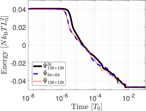
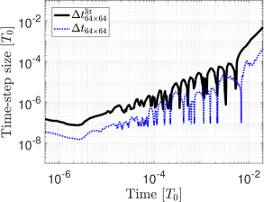
Figure 5: Phase separation on a 2D square. Left: Evolution of the Helmholtz free energy defined in Eq. (64) for $\lambda=1/9000\,L_{0}^{2}$ on meshes containing $64\times 64$ and $128\times 128$ quadratic NURBS elements. Right: Evolution of the time step size. The results for $\bar{\Psi}_{128\times 128}^{\mathrm{lit}}$ and $\Delta t_{64\times 64}^{\mathrm{lit}}$ are taken from Gomez et al., (2008).

7.1.2 Phase separation on a rigid sphere

The second example studies the phase separation on a rigid sphere following the setup of Bartezzaghi et al., (2015). Fig. 6 shows the phase separation over time for this example. Fig. 7 shows the evolution of the free energy compared to the results from Bartezzaghi et al., (2015). The comparison shows a similar evolution in time, but the absolute values are different due to a different normalization of the governing equations.

Figure 6: Phase separation on a rigid sphere. Evolution of the solution for $\lambda=1.3144\cdot 10^{-3}\,L_{0}^{2}$ and volume fraction $\bar{\phi}=0.5$ on a mesh containing $9672$ cubic elements. The coloring follows Table 2.

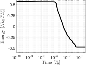
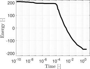
Figure 7: Phase separation on a rigid sphere with $\lambda=1.3144\cdot 10^{-3}\,L_{0}^{2}$ and $\bar{\phi}=0.5$. Left: Evolution of the free energy on a mesh containing $9672$ cubic elements (present result). Right: Evolution of the free energy on a mesh containing $8844$ quadratic NURBS elements (Bartezzaghi et al.,, 2015).

7.2 Phase separation on a deforming torus

The following two examples study phase separations on a deformable torus using the proposed material coupling of Sec. 4.4 and Table 2. A constant internal pressure $p_{\mathrm{int}}=0.1\,EL_{0}^{-1}$ is prescribed for all $t$ to provide mechanical loading. The boundary conditions are illustrated in Fig. 8. This is the first non-trivial example, where both the phase field and surface deformations evolve simultaneously.

Figure 8: Phase separation on a deforming torus: Initial configuration and boundary conditions shown from two different viewpoints. The displacement of six dofs is fixed to prevent rigid body motions.

7.2.1 Large phase interface

The first example studies the behavior of different spatial discretizations with identical initial configurations. A comparison for meshes containing $8\times 32$, $16\times 64$, $32\times 128$, $64\times 256$ and $128\times 512$ quadratic NURBS elements is provided. The mechanical material parameters are listed in Table 2. The mobility constant is selected to be $D=4\,T_{0}$ and the interfacial thickness parameter $\lambda=0.075\,L_{0}^{2}$ is chosen. This is a relatively large value that allows to use coarse meshes: for the coarsest mesh $\sqrt{\lambda}\approx h$ and for the finest mesh $\sqrt{\lambda}\approx 16\,h$, where h is the average element size. The constant internal pressure $p_{\mathrm{int}}=0.1\,EL_{0}^{-1}$ is prescribed for all $t$.

Figure 9: Phase separation on a deforming torus: Evolution of the phase field for $\lambda=0.075\,L_{0}^{2}$ on a deforming torus containing $16\times 64$ quadratic NURBS elements. The coloring follows Table 2.

Fig. 9 shows the evolution of the phase separation over time. The material behavior of phase $\phi=0$ (blue color) is much stiffer than the material behavior of phase $\phi=1$ (red color). Therefore, large bulges appear in the red phase that grow in time as the red phase becomes larger. Fig. 9 also shows that the deformation and phase separation evolve at a similar time scale. The mechanical response is strongly affected by viscosity. Low values of $\eta$ lead to strong oscillations.

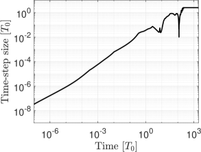
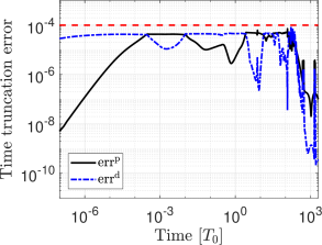
Figure 10: Phase separation on a deforming torus: Left: Time step sizes during phase separation. Right: Evolution of the local time truncation errors for the phase field, $\mathrm{err}^{\mathrm{p}}$, and mechanical field, $\mathrm{err}^{\mathrm{d}}$. The temporal error bound is shown by a red dashed line.

The left side of Fig. 10 shows the time step size resulting from the adaptive time stepping procedure of Sec. 6.5. The right side of Fig. 10 shows the local time truncation errors $\text{err}^{\mathrm{p}}$ and $\text{err}^{\mathrm{d}}$ defined in Eq. (94). It can be observed that the time step is restricted in an alternating manner, by either the mechanical error (dot-dashed blue line) or the phase field error (solid black line). The temporal error bound for rejecting and recomputing the time step is chosen at $10^{-4}$ (red dashed line). The maximum time step size is limited to $\Delta t=2.5\,T_{0}$ to ensure sufficient accuracy and stability.

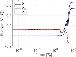
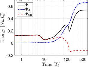
Figure 11: Phase separation on a deforming torus: Evolution of the characteristic energies of the system on the left side (quadratic NURBS, mesh: $16\times 64$). Close-up on the right side.

Fig. 11 shows the evolution of the characteristic energies of the system. Initially, $\bar{\Psi}_{\mathrm{CH}}$ is large compared to $\bar{\Psi}_{\mathrm{el}}$, but then decreases during phase separation due to lowering of $\Psi_{\mathrm{mix}}$ shown in Fig. 1. The kink in Fig. 11 at time $125\,T_{0}$ reflects the state at which the two phases completely separate. At that time the Cahn-Hilliard energy decreases, while the deformation, and thus $\bar{\Psi}_{\mathrm{el}}$, increases with a slight delay due to viscosity. After the phases are completely separated the system reaches a steady state.

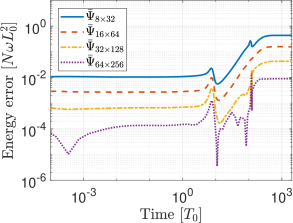
Figure 12: Phase separation on a deforming torus: Left: Evolution of the Helmholtz free energy for five different quadratic NURBS discretizations. Right: Error of the Helmholtz free energy for the coarser meshes $8\times 32$, $16\times 64$, $32\times 128$ and $64\times 256$ with respect to the fine mesh $128\times 512$.

The left side of Fig. 12 shows the evolution of the Helmholtz free energy for the five different NURBS meshes. A good agreement of the evolution of the Helmholtz free energy can be observed for all meshes, except for the coarse meshes $8\times 32$ and $16\times 64$. The right side of Fig. 12 shows the error of the Helmholtz free energy of the coarser meshes with respect to the finest mesh. The error decreases with increasing mesh refinement. After the steady state is reached, the energy error stays constant for all meshes.

7.2.2 Small phase interface

For the second example, $\lambda=0.0075\,L_{0}^{2}$ is selected and the constant internal pressure $p_{\mathrm{int}}=0.1\,EL_{0}^{-1}$ is prescribed for all $t$. The parameters listed in Table 2 and $D=4\,T_{0}$ are used. Fig. 13 shows a series of snapshots of the evolution of the phase field on the deforming torus. Multiple bulges appear, evolve and merge during the phase separation process.

Figure 13: Phase separation on a deforming torus: Evolution of the solution with $\lambda=0.0075\,L_{0}^{2}$ on a mesh containing $32\times 128$ quadratic NURBS elements, with $\sqrt{\lambda}\approx 1.75\,h$. The colors follow Table 2.

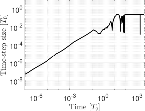
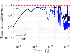
Figure 14: Phase separation on a deforming torus: Left: Adaptive time step sizes. Right: Evolution of the local time truncation errors of the phase field, $\mathrm{err}^{\mathrm{p}}$, and mechanical field, $\mathrm{err}^{\mathrm{d}}$. The temporal error bound is shown by a dashed red line.

Fig. 14 shows the evolution of the time step size and the local truncation error. The time truncation error shows oscillations, which result in abrupt changes of the time step size. This reflects rapid changes and interactions of the phase field and the mechanical field. By choice, the time step size and the local time truncation error are limited to $t=0.25\,T_{0}$ and $10^{-4}$, respectively. Fig. 15 shows the evolution of the characteristic energies of the system. The behavior is similar to the previous example (see Fig. 11).

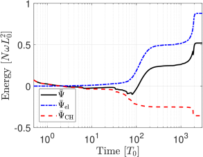
Figure 15: Phase separation on a deforming torus: Evolution of the characteristic energies of the system. Close-up on the right side.

7.3 Phase separation on a deforming sphere

The third example studies phase separation on a deforming sphere that is discretized by the unstructured splines from Sec. 6.1. The parameters $D=4\,T_{0}$ and $\lambda=0.0075\,L_{0}^{2}$ are used together with those in Table 2. The constant internal pressure $p_{\mathrm{int}}=0.0425\,EL_{0}^{-1}$ is prescribed for all $t$. The unstructured mesh consists of $9672$ cubic elements and has $8$ extraordinary points. This mesh provides $C^{2}$-continuity except for the extraordinary points that are only $C^{1}$-continuous. Rigid body deformations are prevented by analogous boundary conditions to those shown in Fig. 8. Fig. 16 shows a series of snapshots of the phase separation on the deforming sphere. Multiple red phase nuclei appear, bulge, evolve and merge during phase separation. As the nuclei grow the deformations become larger.

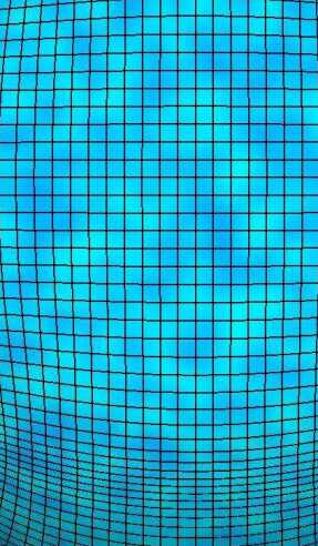
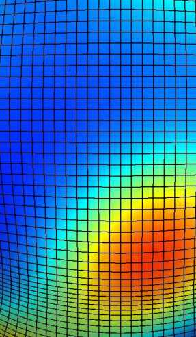
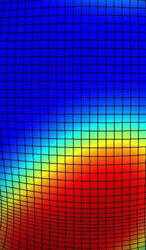
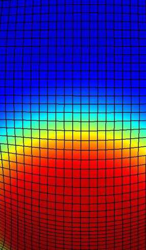
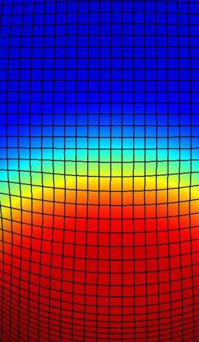
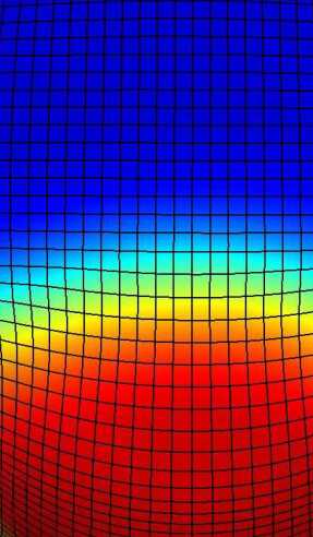
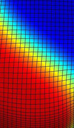
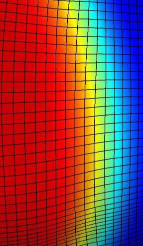
Figure 16: Phase separation on a deforming sphere: Evolution of the solution with $\lambda=0.0075\,L_{0}^{2}$ on an unstructured mesh containing $9672$ cubic elements, with $\sqrt{\lambda}\approx 2.15\,h$. The colors follow Table 2. See also supplemental movie file at https://doi.org/10.5446/40802.

The left side of Fig. 17 shows the evolution of the time step size that results from the adaptive time-stepping procedure of Sec. 6.5. The right side of Fig. 17 shows the local time truncation errors $\text{err}^{\mathrm{p}}$ and $\text{err}^{\mathrm{d}}$. The time step size show similar characteristics as observed in the previous example. The maximum time step size is limited to $\Delta t=0.25\,T_{0}$ in this example. Fig. 18 shows the evolution of the characteristic energies of the system. Like before, in the beginning, $\bar{\Psi}_{\mathrm{CH}}$ is largest. Later, $\bar{\Psi}_{\mathrm{CH}}$ decreases, while $\bar{\Psi}_{\mathrm{el}}$ increases.

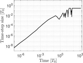
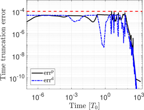
Figure 17: Phase separation on a deforming sphere: Left: Adaptive time step size. Right: Evolution of the local time truncation errors of the phase field, $\mathrm{err}^{\mathrm{p}}$, and mechanical field, $\mathrm{err}^{\mathrm{d}}$. The chosen temporal error bound is shown by a dashed red line.

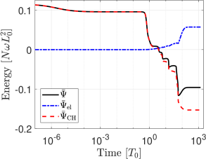
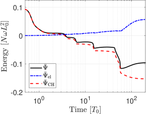
Figure 18: Phase separation on a deforming sphere: Evolution of the characteristic energies of the system. Close-up on the right side.

Next, we illustrate and compare two stress measures: The surface tension

$$\begin{array}[]{l}\gamma_{\bullet}:=\displaystyle\frac{1}{2}N_{\bullet}^{\alpha\beta}\,a_{\alpha\beta}\,,\end{array}$$ (97)

and the deviatoric stress norm

$$\begin{array}[]{l}s_{\bullet}:=\displaystyle\sqrt{N_{\mathrm{dev}}^{\alpha\beta}\,N^{\mathrm{dev}}_{\alpha\beta}}\,,\quad N_{\mathrm{dev}}^{\alpha\beta}:=N^{\alpha\beta}_{\bullet}-\gamma_{\bullet}\,a^{\alpha\beta}\,,\end{array}$$ (98)

that follow from the elastic, viscous and Korteweg stresses introduced in (44) and (49). Note that $N_{\mathrm{visc}}^{\alpha\beta}=\sigma_{\mathrm{visc}}^{\alpha\beta}$ and $N_{\mathrm{CH}}^{\alpha\beta}=\sigma_{\mathrm{CH}}^{\alpha\beta}$. In theory $\gamma_{\mathrm{CH}}=0$ (according to Eq. (47)), while $\gamma_{\mathrm{visc}}\neq 0$ (unless area-incompressibility is assumed). The two stress measures are shown in Fig. 19 and 20.

\begin{overpic}[width=91.0631pt,trim=301.125pt 145.54375pt 762.84999pt 540.01749pt,clip]{ifigs/coup/S/ex_r2/gtot_m8_1650_ts} \put(0.0,0.0){{\color[rgb]{1,1,1}\rule{59.75095pt}{7.82433pt}}} \put(5.0,80.0){$\gamma$} \put(5.0,0.0){$t=21.599\,T_{0}$} \end{overpic}

\begin{overpic}[width=91.0631pt,trim=301.125pt 145.54375pt 762.84999pt 540.01749pt,clip]{ifigs/coup/S/ex_r2/gel_m8_1650_ts} \put(0.0,0.0){{\color[rgb]{1,1,1}\rule{59.75095pt}{7.82433pt}}} \put(5.0,80.0){$\gamma_{\mathrm{el}}$} \put(5.0,0.0){$t=21.599\,T_{0}$} \end{overpic}

\begin{overpic}[width=91.0631pt,trim=301.125pt 145.54375pt 762.84999pt 540.01749pt,clip]{ifigs/coup/S/ex_r2/gk_m8_1650_ts} \put(0.0,0.0){{\color[rgb]{1,1,1}\rule{59.75095pt}{7.82433pt}}} \put(5.0,80.0){$\gamma_{\mathrm{CH}}$} \put(5.0,0.0){$t=21.599\,T_{0}$} \end{overpic}

\begin{overpic}[width=91.0631pt,trim=301.125pt 145.54375pt 762.84999pt 540.01749pt,clip]{ifigs/coup/S/ex_r2/gv_m8_1650_ts} \put(0.0,0.0){{\color[rgb]{1,1,1}\rule{59.75095pt}{7.82433pt}}} \put(5.0,80.0){$\gamma_{\mathrm{visc}}$} \put(5.0,0.0){$t=21.599\,T_{0}$} \end{overpic}

Figure 19: Phase separation on a deforming sphere: Surface tensions $\gamma$, $\gamma_{\mathrm{el}}$, $\gamma_{\mathrm{CH}}$ and $\gamma_{\mathrm{visc}}$ at $t=21.599\,T_{0}$. The colors show the surface tensions in the units $[N\omega]$. See also supplemental movie file at https://doi.org/10.5446/40803.

\begin{overpic}[width=91.0631pt,trim=313.17pt 145.54375pt 717.68124pt 540.01749pt,clip]{ifigs/coup/S/ex_r2/stot_m8_1650_ts} \put(0.0,0.0){{\color[rgb]{1,1,1}\rule{59.75095pt}{7.82433pt}}} \put(5.0,80.0){$s$} \put(5.0,0.0){$t=21.599\,T_{0}$} \end{overpic}

\begin{overpic}[width=91.0631pt,trim=313.17pt 145.54375pt 717.68124pt 540.01749pt,clip]{ifigs/coup/S/ex_r2/sel_m8_1650_ts} \put(0.0,0.0){{\color[rgb]{1,1,1}\rule{59.75095pt}{7.82433pt}}} \put(5.0,80.0){$s_{\mathrm{el}}$} \put(5.0,0.0){$t=21.599\,T_{0}$} \end{overpic}

\begin{overpic}[width=91.0631pt,trim=313.17pt 145.54375pt 717.68124pt 540.01749pt,clip]{ifigs/coup/S/ex_r2/sk_m8_1650_ts} \put(0.0,0.0){{\color[rgb]{1,1,1}\rule{59.75095pt}{7.82433pt}}} \put(5.0,80.0){$s_{\mathrm{CH}}$} \put(5.0,0.0){$t=21.599\,T_{0}$} \end{overpic}

\begin{overpic}[width=91.0631pt,trim=313.17pt 145.54375pt 717.68124pt 540.01749pt,clip]{ifigs/coup/S/ex_r2/sv_m8_1650_ts} \put(0.0,0.0){{\color[rgb]{1,1,1}\rule{59.75095pt}{7.82433pt}}} \put(5.0,80.0){$s_{\mathrm{visc}}$} \put(5.0,0.0){$t=21.599\,T_{0}$} \end{overpic}

Figure 20: Phase separation on a deforming sphere: Stresses $s$, $s_{\mathrm{el}}$, $s_{\mathrm{CH}}$ and $s_{\mathrm{visc}}$ at $t=21.599\,T_{0}$. The colors show the stresses in the units $[N\omega]$. See also supplemental movie file at https://doi.org/10.5446/40804.

The Korteweg stress is largest around bulges at the phase interface. The viscous stress is small in comparison to the Korteweg and elastic stresses. In order to resolve the stress at the phase interface, at least 2 elements should be used per $\sqrt{\lambda}$.

7.4 Phase separation on a deforming double torus

The last example studies phase separation on a deforming double torus, which is discretized by the unstructured splines from Sec. 6.1. The parameters are $D=4\,T_{0}$ and $\lambda=0.025\,L_{0}^{2}$ along with the parameters in Table 2. The constant internal pressure $p_{\mathrm{int}}=0.03\,EL_{0}^{-1}$ is prescribed for all $t$. The unstructured mesh consists of $8264$ cubic elements and has $4$ extraordinary points. As in the previous example, the discretization is $C^{2}$-continuous except for the extraordinary points. Rigid body deformations are prevented by analogous boundary conditions to those shown in Fig. 8. Fig. 21 shows the evolution of the phase separation at various times. The mechanical deformation and the phase field evolve simultaneously and affect each other.

Figure 21: Phase separation on a deforming double torus: Evolution of the solution with $\lambda=0.025\,L_{0}^{2}$ on an unstructured mesh containing $8264$ cubic elements, with $\sqrt{\lambda}\approx 1.6\,h$. The colors follow Table 2.

Fig. 22 shows the evolution of the time step size, which is limited to $\Delta t=T_{0}$, and the local time truncation error. The error restriction of the time step size is alternating similar to the torus case in Sec. 7.2.2. Fig. 23 shows the evolution of the characteristic energies of the system.

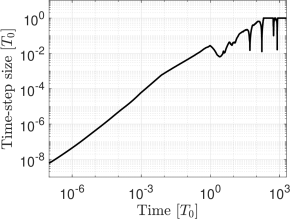
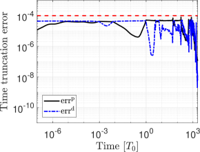
Figure 22: Phase separation on a deforming double torus: Left: Adaptive time step size. Right: Evolution of the local time truncation errors of the phase field, $\mathrm{err}^{\mathrm{p}}$, and mechanical field, $\mathrm{err}^{\mathrm{d}}$. The chosen temporal error bound is shown by a dashed red line.

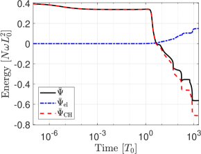
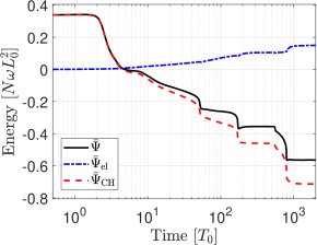
Figure 23: Phase separation on a deforming double torus: Evolution of the characteristic energies of the system. Close-up on the right side.

8 Conclusion

This work presents a novel coupled formulation for the modeling of phase fields on deforming shell surfaces within the framework of isogeometric finite elements. The phase changes are described by the Cahn-Hilliard phase field theory, which is coupled to nonlinear thin shell theory. A phase-dependent material model is presented to describe mixtures. A monolithic and fully implicit time integration scheme is used to solve the coupled system simultaneously. An adaptive time-stepping approach is formulated to adjust the time step size. For the numerical examples, bi-quadratic NURBS discretizations and bi-cubic unstructured quadrilateral spline discretizations are used. Both provide global $C^{1}$-continuity.

The examples presented in Sec. 7 demonstrate the direct coupling of phase transitions and mechanical deformations. The simultaneous evolution of both fields can be observed for the chosen parameters. Other parameters have been observed to produce little or no coupling and they are not reported here for this reason. The adaptive time-stepping approach allows an automatic control of the time step size. The evolution of the phase separation process appears at both small and large time scales. In the absence of fast phase separation and large deformation, the time integration error estimation leads to an almost steady increase of the time step size. Suitable material behavior is required to allow for large deformations and an appropriate interaction of both fields. Due to the direct interaction of mechanical and phase field, the coupled system needs to be damped by viscosity to avoid the build-up of surface oscillations from phase-separation induced deformations. The condition numbers of the tangent matrices of the examples indicate similar observations as in Bartezzaghi et al., (2016): They increase with mesh refinement and with spline order. They decrease with the time step size $\Delta t$. Examining the Newton-Raphson accuracy shows that the present simulation results are not affected by any ill-conditioning (as the Newton-Raphson accuracy reaches machine precision).

Possible extensions of this work include studying applications such as battery systems, liquid droplets and lipid bilayers. The presented shell formulation also applies to liquid menisci (Sauer,, 2014) and lipid bilayers (Katira et al.,, 2016; Sauer et al.,, 2017), but additional numerical tools are needed to handle the coupling of surface flows and phase fields. Another possible extension is the modeling of contact, since large deformations can lead to self-contact. The development of adaptive spatial refinement strategies in order to resolve very thin phase interfaces would also be beneficial. In the future, experiments are also called for in order to calibrate and validate the proposed formulation.

Appendix

Appendix A On the constitutive relations

This section briefly summarizes the derivation of the constitutive equations in Sec. 4.2 and 4.3 following Sahu et al., (2017). The local form of the energy balance on a curved surface can be written as

$$\rho\,\dot{u}=\rho\,r-q^{\alpha}_{;\alpha}+\dfrac{1}{2}\sigma^{\alpha\beta}\dot{a}_{\alpha\beta}+M^{\alpha\beta}\dot{b}_{\alpha\beta}\,,$$ (99)

where $u$ denotes the internal energy density, $r$ is a heat source, $\boldsymbol{q}=q^{\alpha}\boldsymbol{a}_{\alpha}$ is the heat flux on the surface, and $\sigma^{\alpha\beta}$ and $M^{\alpha\beta}$ are stress and bending moment components, respectively. The local form of the entropy balance is

$$\rho\,\dot{s}=-{J_{s}}^{\alpha}_{;\alpha}+\rho\,s_{e}+\rho\,s_{i}\,.$$ (100)

Here, $s$ is the entropy density per unit mass, $J_{s}^{\alpha}$ is the total entropy flux, $s_{e}$ is the total external entropy rate, and $s_{i}$ is the total internal entropy production rate. The second law of thermodynamics dictates that

$$\rho\,s_{i}\geq 0\,.$$ (101)

Let the Helmholtz free energy (per unit mass) be defined as

$$\psi=u-Ts$$ (102)

and assume that it depends on the kinematic variables as

$$\psi=\psi\big{(}a_{\alpha\beta},b_{\alpha\beta},T,\phi,\phi_{;\alpha}\big{)}\,.$$ (103)

Taking a time derivative then gives

$$\begin{array}[]{l}\dot{\psi}=\displaystyle\frac{\partial{\psi}}{\partial{a_{\alpha\beta}}}\dot{a}_{\alpha\beta}+\frac{\partial{\psi}}{\partial{b_{\alpha\beta}}}\dot{b}_{\alpha\beta}+\frac{\partial{\psi}}{\partial{T}}\dot{T}+\frac{\partial{\psi}}{\partial{\phi}}\dot{\phi}+\frac{\partial{\psi}}{\partial{\phi_{;\alpha}}}\dot{\phi}_{;\alpha}\,,\end{array}$$ (104)

which can be rewritten into

$$\begin{array}[]{l}\rho\,\dot{\psi}=\rho\displaystyle\frac{\partial{\psi}}{\partial{a_{\alpha\beta}}}\dot{a}_{\alpha\beta}+\rho\frac{\partial{\psi}}{\partial{b_{\alpha\beta}}}\dot{b}_{\alpha\beta}+\rho\frac{\partial{\psi}}{\partial{T}}\dot{T}+\rho\,\tilde{\mu}_{\mathrm{c}}\,\dot{\phi}+\bigg{(}\rho\frac{\partial{\psi}}{\partial{\phi_{;\alpha}}}\dot{\phi}\bigg{)}_{\!\!;\alpha},\end{array}$$ (105)

where

$$\tilde{\mu}_{\mathrm{c}}:=\frac{\partial{\psi}}{\partial{\phi}}-\frac{1}{\rho}\bigg{(}\rho\frac{\partial{\psi}}{\partial{\phi_{;\alpha}}}\bigg{)}_{\!\!;\alpha}$$ (106)

introduces the chemical potential (per unit mass). From (102) we get

$$\dot{\psi}=\dot{u}-T\dot{s}-\dot{T}s\,,$$ (107)

which can be combined with (99) and (105) to yield

$$\begin{array}[]{lll}\rho\,\dot{s}\!\!\!&=&\!\!\!\displaystyle\dfrac{1}{T}\big{(}\rho r-q^{\alpha}_{;\alpha}\big{)}-\frac{\rho}{T}\bigg{(}s+\frac{\partial\psi}{\partial T}\bigg{)}\dot{T}-\rho\frac{\tilde{\mu}_{\mathrm{c}}}{T}\dot{\phi}-\frac{1}{T}\bigg{(}\rho\frac{\partial{\psi}}{\partial{\phi_{;\alpha}}}\dot{\phi}\bigg{)}_{\!\!;\alpha}\\[11.38109pt] \!\!\!&+&\!\!\!\dfrac{\dot{a}_{\alpha\beta}}{T}\bigg{(}\dfrac{1}{2}\sigma^{\alpha\beta}-\rho\dfrac{\partial\psi}{\partial a_{\alpha\beta}}\bigg{)}+\dfrac{\dot{b}_{\alpha\beta}}{T}\bigg{(}M^{\alpha\beta}-\rho\dfrac{\partial\psi}{\partial b_{\alpha\beta}}\bigg{)}.\end{array}$$ (108)

Let us now assume isothermal conditions such that there are no in-plane temperature gradients ($T_{;\alpha}=0$), and define the entropy as

$$\begin{array}[]{l}s=\displaystyle-\frac{\partial\psi}{\partial T}\,.\end{array}$$ (109)

Substituting the mass balance equation for $\phi$ (18) into (108), we then get

$$\begin{array}[]{lll}\rho\,\dot{s}\!\!\!&=&\!\!\!-\displaystyle\bigg{(}\frac{q^{\alpha}}{T}-\frac{j^{\beta}_{;\beta}}{T}\frac{\partial{\psi}}{\partial{\phi_{;\alpha}}}-\frac{j^{\alpha}\tilde{\mu}_{\mathrm{c}}}{T}\bigg{)}_{\!\!;\alpha}+\dfrac{\rho\,r}{T}\\[11.38109pt] \!\!\!&+&\!\!\!\displaystyle\frac{\dot{a}_{\alpha\beta}}{T}\bigg{(}\frac{1}{2}\sigma^{\alpha\beta}-\rho\dfrac{\partial\psi}{\partial a_{\alpha\beta}}\bigg{)}+\frac{\dot{b}_{\alpha\beta}}{T}\bigg{(}M^{\alpha\beta}-\rho\frac{\partial\psi}{\partial b_{\alpha\beta}}\bigg{)}-\displaystyle\frac{j^{\alpha}\tilde{\mu}_{\mathrm{c};\alpha}}{T}\,.\end{array}$$ (110)

Comparing the above equation with the entropy balance (100) lets us identify the entropy flux

$$J_{s}^{\alpha}=\frac{q^{\alpha}}{T}-\frac{j^{\beta}_{;\beta}}{T}\frac{\partial{\psi}}{\partial{\phi_{;\alpha}}}-\frac{j^{\alpha}\tilde{\mu}_{\mathrm{c}}}{T}\,,$$ (111)

the external entropy rate

$$\rho\,s_{e}=\frac{\rho\,r}{T}$$ (112)

and the total entropy production

$$\rho\,s_{i}=\displaystyle\frac{\dot{a}_{\alpha\beta}}{T}\bigg{(}\frac{1}{2}\sigma^{\alpha\beta}-\rho\dfrac{\partial\psi}{\partial a_{\alpha\beta}}\bigg{)}+\frac{\dot{b}_{\alpha\beta}}{T}\bigg{(}M^{\alpha\beta}-\rho\frac{\partial\psi}{\partial b_{\alpha\beta}}\bigg{)}-\frac{j^{\alpha}\tilde{\mu}_{\mathrm{c};\alpha}}{T}\,,$$ (113)

which has to be positive according to (101). Since $T\geq 0$ and since the quantities $\dot{a}_{\alpha\beta}$, $\dot{b}_{\alpha\beta}$ and $\tilde{\mu}_{\mathrm{c};\alpha}$ can be varied independently, this implies that

$$\dot{a}_{\alpha\beta}\bigg{(}\dfrac{1}{2}\sigma^{\alpha\beta}-\rho\dfrac{\partial\psi}{\partial a_{\alpha\beta}}\bigg{)}\geq 0\quad\forall~{}\dot{a}_{\alpha\beta}$$ (114)

and

$$\dot{b}_{\alpha\beta}\bigg{(}M^{\alpha\beta}-\rho\dfrac{\partial\psi}{\partial b_{\alpha\beta}}\bigg{)}\geq 0\quad\forall~{}\dot{b}_{\alpha\beta}$$ (115)

and

$$-j^{\alpha}\tilde{\mu}_{\mathrm{c};\alpha}\geq 0\,.$$ (116)

If we assume that the bending behavior is purely elastic (such that the bending moments do not depend on the curvature rate $\dot{b}_{\alpha\beta}$), Eq. (115) implies that the bending moments are given by

$$M^{\alpha\beta}=\rho\dfrac{\partial\psi}{\partial b_{\alpha\beta}}\,.$$ (117)

If we assume that the membrane behavior contains an elastic part and a linear viscosity part, Eq. (114) implies that the membrane stresses are given by

$$\sigma^{\alpha\beta}=2\rho\dfrac{\partial\psi}{\partial a_{\alpha\beta}}-\eta\,\dot{a}^{\alpha\beta}\,,$$ (118)

for $\eta\geq 0$. The simplest model satisfying inequality (116) is the linear flux relationship

$$j_{\alpha}=-\tilde{M}\,\tilde{\mu}_{\mathrm{c};\alpha}\,,$$ (119)

as long as $\tilde{M}\geq 0$. These linear models for viscosity and flux are the simplest cases. Alternatively, one can also use nonlinear relationships satisfying (115) and (116). Introducing the initial density $\hat{\rho}=J\rho$ of the undeformed initial mixture, which is considered to be uniform (such that $\hat{\rho}_{;\alpha}=0$ and $\partial\hat{\rho}/\partial\phi=0$), we can define the chemical potential per reference area,

$$\begin{array}[]{l}\mu_{\mathrm{c}}:=\hat{\rho}\,\tilde{\mu}_{\mathrm{c}}=\displaystyle\frac{\partial{\Psi}}{\partial{\phi}}-J\displaystyle\bigg{(}\frac{1}{J}\frac{\partial{\Psi}}{\partial{\phi_{;\alpha}}}\bigg{)}_{\!\!;\alpha},\end{array}$$ (120)

where $\Psi:=\hat{\rho}\,\psi$ is the Helmholtz free energy per reference area, and use this to rewrite

$$j_{\alpha}=-\displaystyle\frac{M}{J}\,\mu_{\mathrm{c};\alpha}\,,$$ (121)

where $M:=\tilde{M}/\rho$. Similarly, $\sigma^{\alpha\beta}$ and $M^{\alpha\beta}$ can be rewritten into the expressions of Eq. (43).

Appendix B Extraction operator initialization

Initializing the extraction operator for a bi-cubic spline function $N$ on an element $\Omega$ is equivalent to defining the polynomial that $N|_{\Omega}$ equals. Choosing the element-local polynomial basis as tensor product Bernstein polynomials $B_{ij}$, we only need to specify coefficients $a_{ij}$ such that,

$$N|_{\Omega}=\sum_{i,j=0}^{3}a_{ij}B_{ij}\;.$$ (122)

Figure 24: A graphical representation of the extraction operator coefficients on a particular Bézier element in the mesh. The coefficient $a_{ij}$ corresponds to the tensor product Bernstein polynomial $B_{ij}$.

In the following, the extraction coefficients $a_{ij}$ will be denoted graphically as shown in Figure 24. Then, the initialization of extraction operators for functions $N_{i}^{D}$ and $N_{i}^{A}$ spanning spline spaces $\mathbb{S}_{D}$ and $\mathbb{S}_{A}$, respectively, is done as follows. (Note that the following assumes all elements to be of uniform size in the parametric domain; this is true for all the numerical results presented in this paper. Please see (Toshniwal et al., 2017b, ) for a more general case.)

• For $\mathbb{S}_{D}$, a basis function is assigned to each vertex of the mesh (black and red disks in Figure 3). The top-left figure in Figure 25 shows the extraction coefficients for the basis function corresponding to the gray disk; $\mu_{i}$ are the number of edges incident on the corners of the element.

• For $\mathbb{S}_{A}$, a basis function is assigned to each regular vertex of the mesh (black disks in Figure 3), and $4$ additional basis functions are assigned to each element containing an extraordinary vertex (blue squares in Figure 3). We call the former vertex-based basis, and the latter face-based basis. The extraction coefficients for them are initialized in a two-step process:

  1. For each vertex-based basis, the extraction coefficients are initialized as per the top-left figure in Figure 25. For each face-based basis, depending on its location w.r.t. the extraordinary point, the extraction coefficients are initialized as per the top-right, mid-left and mid-right figures in Figure 25. (The particular face-based basis being initialized corresponds to the blue square in these figures.)

  2. In order to retain partition of unity, the extraction coefficients for some of the vertex-based basis functions are truncated. Depending on their location w.r.t. the extraordinary point, the extraction coefficients that are set equal to $0$ have been crossed out in the bottom-left and bottom-right figures in Figure 25. (The particular vertex-based basis being truncated corresponds to the gray disk in these figures.)

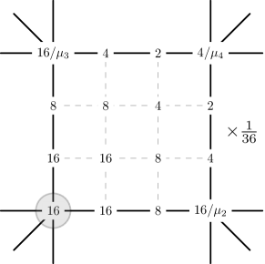
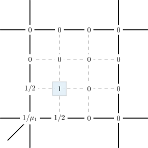
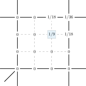
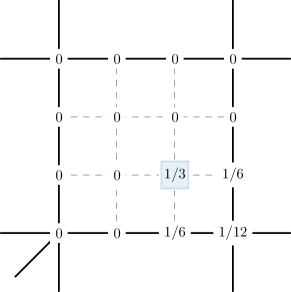
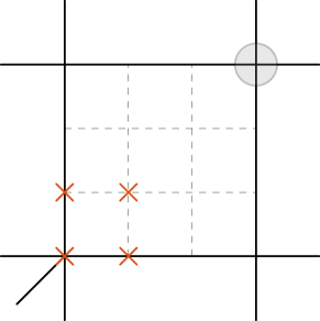
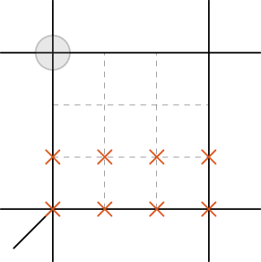
Figure 25: A graphical depiction of the extraction operator initialization. The particular degrees-of-freedom for which the initialization is being performed have been denoted as gray disks or blue squares. The number of edges incident on an element corner has been denoted with $\mu_{i}$; $\mu_{i}\neq 4$ implies an extraordinary point. In all but the top-left figure, the extraordinary point is assumed to coincide with the bottom-left corner of Bézier element. Additionally, it is assumed that an element contains at most one extraordinary point for its corners.

Appendix C Temporal discretization and Newton’s method

Details on the temporal discretization and the iterative solution procedure of Newton’s method are given in this section.

C.1 Generalized-$\alpha$ method

The intermediate quantities, and the quantities at time step $n+1$, are evaluated for the generalized-$\alpha$ method as,

$$\begin{array}[]{lll}\mathbf{x}_{n+1}\!\!\!&=&\!\!\!\mathbf{x}_{n}+\Delta t_{n+1}\,\dot{\mathbf{x}}_{n}+\big{(}\big{(}0.5-\beta\big{)}{\Delta t^{2}_{n+1}}\big{)}\ddot{\mathbf{x}}_{n}+\beta\Delta t^{2}_{n+1}\ddot{\mathbf{x}}_{n+1}\,,\\[5.69054pt] \dot{\mathbf{x}}_{n+1}\!\!\!&=&\!\!\!\dot{\mathbf{x}}_{n}+\big{(}\big{(}1-\gamma\big{)}\Delta t_{n+1}\big{)}\ddot{\mathbf{x}}_{n}+\gamma\Delta t_{n+1}\ddot{\mathbf{x}}_{n+1}\,,\\[5.69054pt] \mathbf{x}_{n+\alpha_{\mathrm{f}}}\!\!\!&=&\!\!\!\big{(}1-\alpha_{\mathrm{f}}\big{)}\mathbf{x}_{n}+\alpha_{\mathrm{f}}\mathbf{x}_{n+1}\,,\\[5.69054pt] \dot{\mathbf{x}}_{n+\alpha_{\mathrm{f}}}\!\!\!&=&\!\!\!\big{(}1-\alpha_{\mathrm{f}}\big{)}\dot{\mathbf{x}}_{n}+\alpha_{\mathrm{f}}\dot{\mathbf{x}}_{n+1}\,,\\[5.69054pt] \ddot{\mathbf{x}}_{n+\alpha_{\mathrm{m}}}\!\!\!&=&\!\!\!\big{(}1-\alpha_{\mathrm{m}}\big{)}\ddot{\mathbf{x}}_{n}+\alpha_{\mathrm{m}}\ddot{\mathbf{x}}_{n+1}\,,\\[5.69054pt] \mbox{\boldmath$\phi$}_{n+1}\!\!\!&=&\!\!\!\mbox{\boldmath$\phi$}_{n}+\Delta t_{n+1}\,\dot{\mbox{\boldmath$\phi$}}_{n}+\gamma\Delta t_{n+1}\left(\dot{\mbox{\boldmath$\phi$}}_{n+1}-\dot{\mbox{\boldmath$\phi$}}_{n}\right)\,,\\[5.69054pt] \mbox{\boldmath$\phi$}_{n+\alpha_{\mathrm{f}}}\!\!\!&=&\!\!\!\big{(}1-\alpha_{\mathrm{f}}\big{)}\mbox{\boldmath$\phi$}_{n}+\alpha_{\mathrm{f}}{\mbox{\boldmath$\phi$}}_{n+1}\,,\\[5.69054pt] \dot{\mbox{\boldmath$\phi$}}_{n+\alpha_{\mathrm{m}}}\!\!\!&=&\!\!\!\big{(}1-\alpha_{\mathrm{m}}\big{)}\dot{\mbox{\boldmath$\phi$}}_{n}+\alpha_{\mathrm{m}}\dot{\mbox{\boldmath$\phi$}}_{n+1}\,,\end{array}$$ (123)

where $\Delta t_{n+1}=t_{n+1}-t_{n}$ is the time step. The algorithmic parameters $\gamma$, $\beta$, $\alpha_{\mathrm{f}}$ and $\alpha_{\mathrm{m}}$ in Eqs. (89) and (123) control numerical dissipation. They can be expressed in terms of $\rho_{\infty}\in[0,1]$, which is an algorithmic parameter corresponding to the spectral radius of the amplification matrix as $\Delta t_{n+1}\rightarrow\infty$, i.e.

$$\begin{array}[]{lll}\alpha_{\mathrm{f}}=\displaystyle\frac{1}{1+\rho_{\infty}}\,,\quad\alpha_{\mathrm{m}}=\displaystyle\frac{2-\rho_{\infty}}{1+\rho_{\infty}}\,,\\[14.22636pt] \gamma=\displaystyle\frac{1}{2}+\alpha_{\mathrm{m}}-\alpha_{\mathrm{f}}\,,\quad\beta=\displaystyle\frac{1}{4}\,(1+\alpha_{\mathrm{m}}-\alpha_{\mathrm{f}})^{2}\,,\end{array}$$ (124)

(see Chung and Hulbert, (1993) for further details). The choice $\rho_{\infty}=0.5$ shows good performance in the subsequent numerical examples.

C.2 Newton-Raphson iteration

Following Bazilevs et al., (2013), the initial guess for the Newton-Raphson iteration is set to

$$\begin{array}[]{lll}\mathbf{x}_{n+1}^{0}=\mathbf{x}_{n}+\Delta t_{n+1}\,\dot{\mathbf{x}}_{n}+\big{(}\big{(}0.5-\beta\big{)}\Delta t^{2}_{n+1}\big{)}\ddot{\mathbf{x}}_{n}+\big{(}\beta\Delta t^{2}_{n+1}\big{)}\ddot{\mathbf{x}}^{0}_{n+1}\,,\\[5.69054pt] \dot{\mathbf{x}}_{n+1}^{0}=\dot{\mathbf{x}}_{n}\,,\\[5.69054pt] \ddot{\mathbf{x}}_{n+1}^{0}=\ddot{\mathbf{x}}_{n}\displaystyle\frac{\gamma-1}{\gamma}\,,\\[5.69054pt] \mbox{\boldmath$\phi$}_{n+1}^{0}=\mbox{\boldmath$\phi$}_{n}~{},\\[5.69054pt] \dot{}\mbox{\boldmath$\phi$}_{n+1}^{0}=\dot{}\mbox{\boldmath$\phi$}_{n}\displaystyle\frac{\gamma-1}{\gamma}\,,\end{array}$$ (125)

and then updated from interation step $i\rightarrow i+1$ by

$$\begin{array}[]{lll}\mathbf{x}_{n+1}^{i+1}=\mathbf{x}_{n+1}^{i}+\Delta\mathbf{x}_{n+1}^{i+1}~{},\\[8.53581pt] \dot{\mathbf{x}}_{n+1}^{i+1}=\dot{\mathbf{x}}_{n+1}^{i}+\Delta\mathbf{x}_{n+1}^{i+1}\displaystyle\frac{1}{\gamma\,\Delta t_{n+1}}\,,\\[8.53581pt] \ddot{\mathbf{x}}_{n+1}^{i+1}=\ddot{\mathbf{x}}_{n+1}^{i}+\Delta\mathbf{x}_{n+1}^{i+1}\displaystyle\frac{1}{\beta\,\Delta t^{2}_{n+1}}\,,\\[8.53581pt] \mbox{\boldmath$\phi$}_{n+1}^{i+1}=\mbox{\boldmath$\phi$}_{n+1}^{i}+\Delta\mbox{\boldmath$\phi$}_{n+1}^{i+1}\,,\\[8.53581pt] \dot{}\mbox{\boldmath$\phi$}_{n+1}^{i+1}=\dot{}\mbox{\boldmath$\phi$}_{n+1}^{i}+\mbox{\boldmath$\phi$}_{n+1}^{i+1}\displaystyle\frac{1}{\gamma\,\Delta t_{n+1}}\,,\end{array}$$ (126)

until convergence is achieved. The stopping criterion for the Newton-Raphson iteration is chosen as

$$\begin{array}[]{l}\text{max}\displaystyle\left\{\frac{\|\mathbf{f}^{i}_{n+1}\|}{\|\mathbf{f}^{0}_{n+1}\|},\frac{\|\bar{\mathbf{f}}^{i}_{n+1}\|}{\|\bar{\mathbf{f}}^{0}_{n+1}\|}\right\}\leq tol^{\mathrm{NR}}~{},\end{array}$$ (127)

where $\|...\|$ denotes the Euclidean norm. The value $tol^{\mathrm{NR}}=10^{-4}$ is observed to be sufficient for all examples to ensure convergence. This algorithm is also known as a predictor-multicorrector algorithm, with (125) as the prediction and (126) as the multicorrection.

Remark: The choices (125), (126) show good convergence of Newton’s method for fluid structure interaction applications (Bazilevs et al.,, 2013), and good convergence is also achieved for the examples in this work.

Appendix D Linearization

The linearization of the mechanical force vector $\mathbf{f}^{e}:=\mathbf{f}^{e}_{\mathrm{in}}+\mathbf{f}^{e}_{\mathrm{int}}-\mathbf{f}^{e}_{\mathrm{ext}}$ of finite element $\Omega^{e}$ (81) with respect to the nodal positions of $\Omega^{e}$, $\mathbf{x}_{e}$, can be found in Duong et al., (2017). The linearization of $\mathbf{f}^{e}$ with respect to the nodal phase variables of $\Omega^{e}$, $\mbox{\boldmath$\phi$}_{e}$, according to (81), is

$$\begin{array}[]{lll}\Delta_{\phi}\mathbf{f}^{e}=\big{[}{\mathbf{k}}^{e}_{\sigma\phi}+{\mathbf{k}}^{e}_{M\phi}\big{]}\,\Delta\mbox{\boldmath$\phi$}_{e}\,,\end{array}$$ (128)

with

$$\begin{array}[]{lll}{\mathbf{k}}^{e}_{\sigma\phi}\!\!\!&:=&\!\!\!\displaystyle\int_{\Omega_{0}^{e}}\frac{\partial\tau^{\alpha\beta}}{\partial\phi}\,\mathbf{N}^{\mathrm{T}}_{\!,\alpha}\,\boldsymbol{a}^{h}_{\beta}\,\bar{\mathbf{N}}\,\mathrm{d}A+\displaystyle\int_{\Omega_{0}^{e}}\frac{\partial\tau^{\alpha\beta}}{\partial\phi_{;\gamma}}\,\mathbf{N}^{\mathrm{T}}_{\!,\alpha}\,\boldsymbol{a}^{h}_{\beta}\,\bar{\mathbf{N}}_{\!,\gamma}\,\mathrm{d}A\,,\\[11.38109pt] {\mathbf{k}}^{e}_{M\phi}\!\!\!&:=&\!\!\!\displaystyle\int_{\Omega_{0}^{e}}\frac{\partial M_{0}^{\alpha\beta}}{\partial\phi}\,\mathbf{N}^{\mathrm{T}}_{\!;\alpha\beta}\,\boldsymbol{n}^{h}\,\bar{\mathbf{N}}\,\mathrm{d}A\,,\end{array}$$ (129)

where $\tau^{\alpha\beta}:=J\sigma^{\alpha\beta}$ and $M^{\alpha\beta}_{0}:=JM^{\alpha\beta}$. According to Sec. 4.3, we find

$$\begin{array}[]{lll}\displaystyle\frac{\partial{\tau^{\alpha\beta}}}{\partial{\phi}}\!\!\!&=&\!\!\!\displaystyle\frac{K^{\prime}}{2}\left(J^{2}-1\right)a^{\alpha\beta}+\frac{G^{\prime}}{2\,J}\left(2\,A^{\alpha\beta}-I_{1}\,a^{\alpha\beta}\right)-J\,\eta^{\prime}\,\dot{a}^{\alpha\beta}\,,\\[11.38109pt] \displaystyle\frac{\partial{\tau^{\alpha\beta}}}{\partial{\phi_{;\gamma}}}\!\!\!&=&\!\!\!J\lambda\left(a^{\alpha\beta}\,a^{\gamma\delta}-a^{\alpha\gamma}\,a^{\beta\delta}-a^{\alpha\delta}\,a^{\beta\gamma}\right)\phi_{;\delta}\,,\\[11.38109pt] \displaystyle\frac{\partial{M_{0}^{\alpha\beta}}}{\partial{\phi}}\!\!\!&=&\!\!\!\displaystyle c^{\prime}\left(A^{\alpha\gamma}\,b_{\gamma\delta}\,A^{\beta\delta}-B^{\alpha\beta}\right)\,.\end{array}$$ (130)

According to Eq. (88), the linearization of $\bar{\mathbf{f}}^{e}$ with respect to the nodal positions of $\Omega^{e}$, $\mathbf{x}_{e}$, is

$$\begin{array}[]{lll}\Delta_{\mathrm{x}}\bar{\mathbf{f}}^{e}=\Delta_{\mathrm{x}}\bar{\mathbf{f}}^{e}_{\mathrm{int}}\,.\end{array}$$ (131)

Since we can write

$$\begin{array}[]{lll}\bar{\mathbf{f}}^{e}_{\mathrm{int}}=\displaystyle\int_{\Omega^{e}_{0}}\Big{[}\bar{\mathbf{N}}_{\!,\alpha}^{\mathrm{T}}\,a^{\alpha\beta}\Big{(}\!M\mu^{\prime}_{\phi}-M^{\prime}\big{(}\mu_{\mathrm{i}}+\mu_{\mathrm{el}}\big{)}\!\Big{)}\,\phi_{;\beta}-\Delta_{\mathrm{s}}\bar{\mathbf{N}}^{\mathrm{T}}M\big{(}\mu_{\mathrm{i}}+\mu_{\mathrm{el}}\Big{)}\Big{]}\,\mathrm{d}A\end{array}$$ (132)

where $\mu_{\bullet}$ are the contributions given in (39), we obtain

$$\begin{array}[]{lll}\Delta_{\mathrm{x}}\bar{\mathbf{f}}^{e}=\Delta_{\mathrm{x}}\bar{\mathbf{f}}^{e}_{\mathrm{x}1}+\Delta_{\mathrm{x}}\bar{\mathbf{f}}^{e}_{\mathrm{x}2}+\Delta_{\mathrm{x}}\bar{\mathbf{f}}^{e}_{\mathrm{x}3}\,,\end{array}$$ (133)

with

$$\begin{array}[]{lll}\Delta_{\mathrm{x}}\bar{\mathbf{f}}^{e}_{\mathrm{x1}}\!\!\!&=&\!\!\!\displaystyle\int_{\Omega^{e}_{0}}\bar{\mathbf{N}}_{\!,\alpha}^{\mathrm{T}}\Big{(}\!M\mu^{\prime}_{\phi}-M^{\prime}\big{(}\mu_{\mathrm{i}}+\mu_{\mathrm{el}}\big{)}\!\Big{)}\,\phi_{;\beta}\,\Delta a^{\alpha\beta}\,\mathrm{d}A\,,\\[11.38109pt] \Delta_{\mathrm{x}}\bar{\mathbf{f}}^{e}_{\mathrm{x2}}\!\!\!&=&\!\!\!-\displaystyle\int_{\Omega^{e}_{0}}\Big{(}\bar{\mathbf{N}}_{\!,\alpha}^{\mathrm{T}}\,a^{\alpha\beta}\,\phi_{;\beta}\,M^{\prime}+\Delta_{\mathrm{s}}\bar{\mathbf{N}}^{\mathrm{T}}M\Big{)}\big{(}\Delta_{\mathrm{x}}\mu_{\mathrm{i}}+\Delta_{\mathrm{x}}\mu_{\mathrm{el}}\big{)}\,\mathrm{d}A\,,\\[11.38109pt] \Delta_{\mathrm{x}}\bar{\mathbf{f}}^{e}_{\mathrm{x3}}\!\!\!&=&\!\!\!-\displaystyle\int_{\Omega^{e}_{0}}M\big{(}\mu_{\mathrm{i}}+\mu_{\mathrm{el}}\big{)}\,\Delta\Delta_{\mathrm{s}}\bar{\mathbf{N}}^{\mathrm{T}}\,\mathrm{d}A\,.\\[11.38109pt] \end{array}$$ (134)

According to Sauer et al., (2014) and Sauer and Duong, (2017) we have

$$\begin{array}[]{lll}\Delta\boldsymbol{a}_{\alpha}\!\!\!&=&\!\!\!\mathbf{N}_{\!,\alpha}\,\Delta\mathbf{x}_{e}\,,\\[5.69054pt] \Delta\boldsymbol{a}_{\alpha,\beta}\!\!\!&=&\!\!\!\mathbf{N}_{\!,\alpha\beta}\,\Delta\mathbf{x}_{e}\,,\\[5.69054pt] \Delta J\!\!\!&=&\!\!\!J\boldsymbol{a}^{\alpha}\cdot\mathbf{N}_{\!,\alpha}\,\Delta\mathbf{x}_{e}\,,\\[5.69054pt] \Delta a^{\alpha\beta}\!\!\!&=&\!\!\!-\big{(}\boldsymbol{a}^{\alpha}a^{\beta\gamma}+\boldsymbol{a}^{\beta}a^{\alpha\gamma}\big{)}\cdot\mathbf{N}_{\!,\gamma}\,\Delta\mathbf{x}_{e}\,,\\[5.69054pt] \Delta\boldsymbol{a}^{\alpha}\!\!\!&=&\!\!\!\big{(}a^{\alpha\beta}\boldsymbol{n}\otimes\boldsymbol{n}-\boldsymbol{a}^{\beta}\otimes\boldsymbol{a}^{\alpha})\cdot\mathbf{N}_{\!,\beta}\,\Delta\mathbf{x}_{e}\,.\end{array}$$ (135)

With this we find

$$\begin{array}[]{l}\Delta\Gamma^{\gamma}_{\alpha\beta}=\big{(}\boldsymbol{a}^{\gamma}\cdot\mathbf{N}_{;\alpha\beta}+a^{\gamma\delta}\boldsymbol{a}_{\alpha;\beta}\cdot\mathbf{N}_{\!,\delta}\big{)}\,\Delta\mathbf{x}_{e}\,,\end{array}$$ (136)

and thus

$$\begin{array}[]{l}a^{\alpha\beta}\,\Delta\Gamma^{\gamma}_{\alpha\beta}=\mathbf{N}^{\gamma}\,\Delta\mathbf{x}_{e}\,,\end{array}$$ (137)

where

$$\begin{array}[]{l}\mathbf{N}^{\gamma}:=a^{\alpha\beta}\,\boldsymbol{a}^{\gamma}\cdot\mathbf{N}_{;\alpha\beta}+2H\,a^{\gamma\delta}\,\boldsymbol{n}\cdot\mathbf{N}_{\!,\delta}\,.\end{array}$$ (138)

From this follows

$$\begin{array}[]{l}\Delta\Delta_{\mathrm{s}}\bar{\mathbf{N}}^{\mathrm{T}}=\mathbf{M}_{\Delta_{\mathrm{s}}}\,\Delta\mathbf{x}_{e}\,,\end{array}$$ (139)

where

$$\begin{array}[]{l}\mathbf{M}_{\Delta_{\mathrm{s}}}:=\displaystyle-2\,\bar{\mathbf{N}}^{\mathrm{T}}_{;\alpha\beta}\,\boldsymbol{a}^{\alpha}\,a^{\beta\gamma}\cdot\mathbf{N}_{\!,\gamma}-\bar{\mathbf{N}}^{\mathrm{T}}_{\!,\gamma}\,\mathbf{N}^{\gamma}\,.\end{array}$$ (140)

Hence $\Delta_{\mathrm{x}}\Delta_{\mathrm{s}}\phi=\mbox{\boldmath$\phi$}_{e}^{\mathrm{T}}\,\mathbf{M}_{\Delta_{\mathrm{s}}}\,\Delta\mathbf{x}_{e}$ and

$$\begin{array}[]{l}\Delta_{\mathrm{x}}\mu_{\mathrm{i}}=\mathbf{N}_{\mathrm{i}}\,\Delta\mathbf{x}_{e}\,,\end{array}$$ (141)

with

$$\begin{array}[]{l}\mathbf{N}_{\mathrm{i}}:=\mu_{\mathrm{i}}\,\boldsymbol{a}^{\alpha}\cdot\mathbf{N}_{\!,\alpha}-J\lambda\,\mbox{\boldmath$\phi$}_{e}^{\mathrm{T}}\,\mathbf{M}_{\Delta_{\mathrm{s}}}\,.\end{array}$$ (142)

Similarly, we have

$$\begin{array}[]{l}\Delta_{\mathrm{x}}\mu_{\mathrm{el}}=\mathbf{N}_{\mathrm{el}}\,\Delta\mathbf{x}_{e}\,,\end{array}$$ (143)

with

$$\begin{array}[]{l}\mathbf{N}_{\mathrm{el}}:={\tau^{\alpha\beta}_{\mathrm{el}}}^{\prime}\boldsymbol{a}_{\alpha}\cdot\mathbf{N}_{\!,\beta}+{M^{\alpha\beta}_{0}}^{\prime}\boldsymbol{n}\cdot\mathbf{N}_{\!;\alpha\beta}\,,\end{array}$$ (144)

since

$$\begin{array}[]{lll}\displaystyle\frac{\partial{\mu_{\mathrm{el}}}}{\partial{a_{\alpha\beta}}}\!\!\!&=&\!\!\!\displaystyle\frac{\partial{\tau^{\alpha\beta}_{\mathrm{el}}}}{\partial{\phi}}:={\tau^{\alpha\beta}_{\mathrm{el}}}^{\prime}\,,\\[11.38109pt] \displaystyle\frac{\partial{\mu_{\mathrm{el}}}}{\partial{b_{\alpha\beta}}}\!\!\!&=&\!\!\!\displaystyle\frac{\partial{M^{\alpha\beta}_{0}}}{\partial{\phi}}:={M^{\alpha\beta}_{0}}^{\prime}\,.\end{array}$$ (145)

We can thus write

$$\begin{array}[]{lll}\Delta_{\mathrm{x}}\bar{\mathbf{f}}^{e}=\big{[}\bar{\mathbf{k}}^{e}_{\mathrm{x}1}+\bar{\mathbf{k}}^{e}_{\mathrm{x}2}+\bar{\mathbf{k}}^{e}_{\mathrm{x}3}\big{]}\,\Delta\mathbf{x}_{e}\,,\end{array}$$ (146)

where

$$\begin{array}[]{lll}\bar{\mathbf{k}}^{e}_{\mathrm{x}1}\!\!\!&:=&\!\!\!-\displaystyle\int_{\Omega^{e}_{0}}\left(M\,\mu^{\prime}_{\phi}-M^{\prime}\,\left(\mu_{i}\,+\mu_{\mathrm{el}}\right)\right)\bar{\mathbf{N}}^{\mathrm{T}}_{\!,\alpha}\,\phi_{;\beta}\big{(}\boldsymbol{a}^{\alpha}a^{\beta\gamma}+\boldsymbol{a}^{\beta}a^{\alpha\gamma}\big{)}\cdot\mathbf{N}_{\!,\gamma}\,\mathrm{d}A\,,\\[11.38109pt] \bar{\mathbf{k}}^{e}_{\mathrm{x}2}\!\!\!&:=&\!\!\!-\displaystyle\int_{\Omega^{e}_{0}}\Big{(}\bar{\mathbf{N}}_{\!,\alpha}^{\mathrm{T}}\,a^{\alpha\beta}\,\phi_{;\beta}\,M^{\prime}+\Delta_{\mathrm{s}}\bar{\mathbf{N}}^{\mathrm{T}}M\Big{)}\big{(}\mathbf{N}_{\mathrm{i}}+\mathbf{N}_{\mathrm{el}}\big{)}\,\mathrm{d}A\,,\\[11.38109pt] \bar{\mathbf{k}}^{e}_{\mathrm{x}3}\!\!\!&:=&\!\!\!\displaystyle-\int_{\Omega^{e}_{0}}M\big{(}\mu_{\mathrm{i}}+\mu_{\mathrm{el}}\big{)}\,\mathbf{M}_{\Delta_{\mathrm{s}}}\,\mathrm{d}A\,.\end{array}$$ (147)

The linearization of $\bar{\mathbf{f}}^{e}$ with respect to the phase variables of $\Omega^{e}$, $\mbox{\boldmath$\phi$}_{e}$, according to (88), is

$$\begin{array}[]{lll}\Delta_{\phi}\bar{\mathbf{f}}_{\mathrm{int}}^{e}=\displaystyle\big{[}\bar{\mathbf{k}}^{e}+\bar{\mathbf{k}}_{\phi 1}^{e}+\bar{\mathbf{k}}_{\phi 2}^{e}+\bar{\mathbf{k}}_{\phi 3}^{e}\big{]}\,\Delta\mbox{\boldmath$\phi$}_{e}~{},\end{array}$$ (148)

with $\bar{\mathbf{k}}^{e}$ given in (88), and

$$\begin{array}[]{lll}\bar{\mathbf{k}}_{\phi 1}^{e}=\displaystyle\int_{\Omega^{e}_{0}}\bar{\mathbf{N}}_{,\alpha}^{\mathrm{T}}\,a^{\alpha\beta}\,\phi_{,\beta}\left(M^{\prime}\left(\mu^{\prime}_{\phi}-\mu^{\prime}_{\mathrm{el}}\right)+M\,\mu^{\prime\prime}_{\phi}-M^{\prime\prime}\left(\mu_{\mathrm{i}}+\mu_{\mathrm{el}}\right)\right)\,\bar{\mathbf{N}}\,\mathrm{d}A\,,\\[11.38109pt] \bar{\mathbf{k}}_{\phi 2}^{e}=\displaystyle\int_{\Omega^{e}_{0}}\bar{\mathbf{N}}_{,\alpha}^{\mathrm{T}}\,a^{\alpha\beta}\,\phi_{,\beta}\,J\lambda\,M^{\prime}\,\Delta_{\mathrm{s}}\bar{\mathbf{N}}\,\mathrm{d}A\,,\\[11.38109pt] \bar{\mathbf{k}}_{\phi 3}^{e}=-\displaystyle\int_{\Omega^{e}_{0}}\Delta_{\mathrm{s}}\bar{\mathbf{N}}^{\mathrm{T}}\,\left(M^{\prime}\,(\mu_{\mathrm{i}}+\mu_{\mathrm{el}})+M\,\mu^{\prime}_{\mathrm{el}}\right)\bar{\mathbf{N}}\,\mathrm{d}A\,.\end{array}$$ (149)

Appendix E Error estimation

E.1 Error estimates for the mechanical field

As proposed in Hulbert and Jang, (1995), the local error of the deformation and the velocity is given by

$$\begin{array}[]{lll}\boldsymbol{e}^{d}_{n+1}=\mathbf{x}_{n+1}-\hat{\mathbf{x}}_{n+1}\,,\qquad\boldsymbol{e}^{v}_{n+1}=\dot{\mathbf{x}}_{n+1}-\dot{\hat{\mathbf{x}}}_{n+1}\,,\end{array}$$ (150)

where $\hat{\mathbf{x}}_{n+1}:=\hat{\mathbf{x}}_{n+1}(t_{n+1})$ and $\dot{\hat{\mathbf{x}}}_{n+1}:=\dot{\hat{\mathbf{x}}}_{n+1}(t_{n+1})$ are the solutions of the local problem. Expressions for $\hat{\mathbf{x}}_{n+1}$ and $\dot{\hat{\mathbf{x}}}_{n+1}$ are obtained by a Taylor series with finite remainder about $t_{n}$ (Appendix E.3, Eq. (172)). At time $t_{n}$, $\mathbf{x}_{n}=\hat{\mathbf{x}}_{n}$ and $\dot{\mathbf{x}}_{n}=\dot{\hat{\mathbf{x}}}_{n}$ holds. Using the Newmark formulae (Eq. (174)) for $\mathbf{x}_{n+1}$ and $\dot{\mathbf{x}}_{n+1}$, the local errors can be expressed as

$$\begin{array}[]{lll}\boldsymbol{e}^{d}_{n+1}=\displaystyle\Delta t_{n+1}^{2}\left(\beta\Delta\ddot{\mathbf{x}}_{n}-\frac{1}{6}\Delta t_{n+1}\dddot{\hat{\mathbf{x}}}(\xi_{u})+\frac{1}{2}\left(\ddot{\mathbf{x}}_{n}-\ddot{\hat{\mathbf{x}}}_{n}\right)\right)\,,\\[11.38109pt] \boldsymbol{e}^{v}_{n+1}=\displaystyle\Delta t_{n+1}\left(\gamma\Delta\ddot{\mathbf{x}}_{n}-\frac{1}{2}\Delta t_{n+1}\dddot{\hat{\mathbf{x}}}(\xi_{v})+\left(\ddot{\mathbf{x}}_{n}-\ddot{\hat{\mathbf{x}}}_{n}\right)\right)\,,\end{array}$$ (151)

where $\Delta\ddot{\mathbf{x}}_{n}:=\ddot{\mathbf{x}}_{n+1}-\ddot{\mathbf{x}}_{n}$. Values for $\dddot{\hat{\mathbf{x}}}(\xi_{u})$ and $\dddot{\hat{\mathbf{x}}}(\xi_{v})$ with $\xi_{u},\xi_{v}\in[t_{n},t_{n+1}]$ are obtained by the following approximation

$$\begin{array}[]{lll}\dddot{\hat{\mathbf{x}}}(\xi_{u})=\dddot{\hat{\mathbf{x}}}(\xi_{v})\approx\Delta t_{n+1}^{-1}\left(\ddot{\hat{\mathbf{x}}}_{n+1}-\ddot{\hat{\mathbf{x}}}_{n}\right)\,.\end{array}$$ (152)

Substituting Eq. (151) into (150) and employing the results in the basic form of the generalized-$\alpha$ method

$$\begin{array}[]{lll}\mathbf{M}\ddot{\mathbf{x}}_{n+1-\alpha_{\mathrm{m}}}+\mathbf{f}_{\mathrm{int}}(\mathbf{x}_{n+1-\alpha_{\mathrm{f}}},\dot{\mathbf{x}}_{n+1-\alpha_{\mathrm{f}}})-\mathbf{f}_{\mathrm{ext}}(\mathbf{x}_{n+1-\alpha_{\mathrm{f}}},\dot{\mathbf{x}}_{n+1-\alpha_{\mathrm{f}}},t_{n+1-\alpha_{\mathrm{f}}})=\boldsymbol{0}\,,\end{array}$$ (153)

results in

$$\begin{array}[]{lll}\mathbf{M}(\ddot{\mathbf{x}}_{n+1}-\ddot{\hat{\mathbf{x}}}_{n+1})=\alpha_{\mathrm{m}}\mathbf{M}\Delta\ddot{\mathbf{x}}_{n}-\alpha_{\mathrm{f}}\mathbf{M}\Delta\ddot{\hat{\mathbf{x}}}_{n}-(1-\alpha_{\mathrm{f}})\mathbf{K}_{\mathrm{x}}\boldsymbol{e}^{d}_{n+1}-(1-\alpha_{\mathrm{f}})\mathbf{C}\boldsymbol{e}^{v}_{n+1}\,.\end{array}$$ (154)

Note, that Eq. (153) is solved at intermediate time steps and we use

$$\begin{array}[]{lll}\mathbf{x}_{n+1-\alpha_{\mathrm{f}}}=(1-\alpha_{\mathrm{f}})\mathbf{x}_{n+1}+\alpha_{\mathrm{f}}\mathbf{x}_{n}\,,\\[11.38109pt] \dot{\mathbf{x}}_{n+1-\alpha_{\mathrm{f}}}=(1-\alpha_{\mathrm{f}})\dot{\mathbf{x}}_{n+1}+\alpha_{\mathrm{f}}\dot{\mathbf{x}}_{n}\,,\\[11.38109pt] \ddot{\mathbf{x}}_{n+1-\alpha_{\mathrm{m}}}=(1-\alpha_{\mathrm{m}})\ddot{\mathbf{x}}_{n+1}+\alpha_{\mathrm{m}}\ddot{\mathbf{x}}_{n}\,.\end{array}$$ (155)

Replacing $n$ by $n-1$, and after some algebraic manipulations, we obtain

$$\begin{array}[]{lll}(1-\alpha_{\mathrm{f}})\mathbf{M}\Delta\ddot{\hat{\mathbf{x}}}_{n}=\mathbf{M}\left((1-\alpha_{\mathrm{m}})\Delta\ddot{\mathbf{x}}_{n}+\alpha_{\mathrm{m}}\Delta\ddot{\mathbf{x}}_{n-1}-\alpha_{\mathrm{f}}\Delta\ddot{\hat{\mathbf{x}}}_{n-1}\right)+(1-\alpha_{\mathrm{f}})(\mathbf{K}_{\mathrm{x}}\Delta\boldsymbol{e}^{d}_{n}+\mathbf{C}\Delta\boldsymbol{e}^{v}_{n})\,,\\[11.38109pt] \mathbf{M}(\ddot{\mathbf{x}}_{n}-\ddot{\hat{\mathbf{x}}}_{n})=(1-\alpha_{\mathrm{f}})\mathbf{M}\Delta\ddot{\hat{\mathbf{x}}}_{n}-(1-\alpha_{\mathrm{m}})\mathbf{M}\Delta\ddot{\mathbf{x}}_{n}-(1-\alpha_{\mathrm{f}})(\mathbf{K}_{\mathrm{x}}\boldsymbol{e}^{d}_{n+1}-\mathbf{C}\boldsymbol{e}^{v}_{n+1})\,.\end{array}$$ (156)

Multiplying Eq. (151) by $\mathbf{M}$ and using Eq. (156) results in

$$\begin{array}[]{lll}\begin{bmatrix}\displaystyle\mathbf{M}+\frac{1}{6}\Delta t^{2}_{n+1}\mathbf{K}_{\mathrm{x}}&\displaystyle\frac{1}{6}\Delta t^{2}_{n+1}\boldsymbol{C}\\[11.38109pt] \displaystyle\frac{1}{2}\Delta t^{2}_{n+1}\mathbf{K}_{\mathrm{x}}&\displaystyle\mathbf{M}+\frac{1}{2}\Delta t^{2}_{n+1}\mathbf{C}\end{bmatrix}\begin{bmatrix}\displaystyle\boldsymbol{e}^{d}_{n+1}\\[11.38109pt] \displaystyle\Delta t_{n+1}\boldsymbol{e}^{v}_{n+1}\end{bmatrix}=\\[34.1433pt] \Delta t_{n+1}^{2}\begin{bmatrix}\displaystyle\left(\left(\beta-\frac{1-\alpha_{\mathrm{m}}}{6\left(1-\alpha_{\mathrm{f}}\right)}\right)\Delta\ddot{\mathbf{x}}_{n}+\left(\frac{1}{6\left(1-\alpha_{\mathrm{f}}\right)}-\frac{1}{2}\right)\boldsymbol{w}_{n}\right)\\[11.38109pt] \displaystyle\left(\left(\gamma-\frac{1-\alpha_{\mathrm{m}}}{2\left(1-\alpha_{\mathrm{f}}\right)}\right)\Delta\ddot{\mathbf{x}}_{n}+\left(\frac{1}{2\left(1-\alpha_{\mathrm{f}}\right)}-1\right)\boldsymbol{w}_{n}\right)\end{bmatrix}+\\[34.1433pt] \Delta t_{n+1}^{2}\begin{bmatrix}\displaystyle\left(\frac{1}{2}\alpha_{\mathrm{f}}-\frac{1}{3}\right)\left(\mathbf{K}_{\mathrm{x}}\boldsymbol{e}^{d}_{n}+\mathbf{C}\boldsymbol{e}^{v}_{n}\right)\\[11.38109pt] \displaystyle\left(\alpha_{\mathrm{f}}-\frac{1}{2}\right)\left(\mathbf{K}_{\mathrm{x}}\boldsymbol{e}^{d}_{n}+\mathbf{C}\boldsymbol{e}^{v}_{n}\right)\end{bmatrix}\,,\end{array}$$ (157)

with

$$\begin{array}[]{lll}\boldsymbol{w}_{n}=\alpha_{\mathrm{m}}\Delta\ddot{\mathbf{x}}_{n-1}-\alpha_{\mathrm{f}}\Delta\ddot{\hat{\mathbf{x}}}_{n-1}\,.\end{array}$$ (158)

Dropping the higher order terms, $\Delta t_{n+1}^{2}\mathbf{K}_{\mathrm{x}}$ and $\Delta t_{n+1}\mathbf{C}$, the local errors are expressed as

$$\begin{array}[]{lll}\boldsymbol{e}_{n+1}^{d}=\displaystyle\Delta t_{n+1}^{2}\left(\left(\beta-\frac{1-\alpha_{\mathrm{m}}}{6\left(1-\alpha_{\mathrm{f}}\right)}\right)\Delta\ddot{\mathbf{x}}_{n}+\left(\frac{1}{6\left(1-\alpha_{\mathrm{f}}\right)}-\frac{1}{2}\right)\boldsymbol{w}_{n}\right)\,,\\[11.38109pt] \boldsymbol{e}_{n+1}^{v}=\displaystyle\Delta t_{n+1}\left(\left(\gamma-\frac{1-\alpha_{\mathrm{m}}}{2\left(1-\alpha_{\mathrm{f}}\right)}\right)\Delta\ddot{\mathbf{x}}_{n}+\left(\frac{1}{2\left(1-\alpha_{\mathrm{f}}\right)}-1\right)\boldsymbol{w}_{n}\right)\,.\end{array}$$ (159)

Rewriting $\boldsymbol{w}_{n}$ into

$$\begin{array}[]{lll}\boldsymbol{w}_{n}=\displaystyle\frac{\alpha_{\mathrm{m}}-\alpha_{\mathrm{f}}}{(1-\alpha_{\mathrm{f}})^{2}}\Delta\ddot{\mathbf{x}}_{n}-\frac{\alpha_{\mathrm{f}}}{1-\alpha_{\mathrm{f}}}\boldsymbol{w}_{n-1},\quad\text{with}\quad\boldsymbol{w}_{0}=\boldsymbol{0}\,,\end{array}$$ (160)

following the idea of Hulbert and Jang, (1995) and interpreting $\boldsymbol{w}_{n}$ as a history vector, Eq. (159) can be expressed as Eq. (92) with constants

$$\begin{array}[]{lll}c_{1}^{\mathrm{d}}=\displaystyle\beta-\frac{1-\alpha_{\mathrm{m}}}{6\left(1-\alpha_{\mathrm{f}}\right)}\,,\qquad c_{2}^{\mathrm{d}}=\displaystyle\left(1+\rho_{\infty}\right)\left(1-\rho_{\infty}\right)\left(\frac{1}{6}-\frac{1}{2}\left(1-\alpha_{\mathrm{f}}\right)\right)\,.\end{array}$$ (161)

E.2 Error estimate for the phase field

The local error of the phase field is given by

$$\begin{array}[]{lll}\boldsymbol{e}^{p}_{n+1}=\mbox{\boldmath$\phi$}_{n+1}-\hat{}\mbox{\boldmath$\phi$}_{n+1}\,.\end{array}$$ (162)

By following the same approach as for the mechanical field, Eq. (162) can be expressed as

$$\begin{array}[]{lll}\boldsymbol{e}^{p}_{n+1}=\displaystyle\Delta t_{n+1}\left(\gamma\Delta\dot{\mbox{\boldmath$\phi$}}_{n}-\frac{1}{2}\Delta t_{n+1}\ddot{\hat{}\mbox{\boldmath$\phi$}}(\xi_{\phi})+\left(\dot{\mbox{\boldmath$\phi$}}_{n}-\dot{\hat{}\mbox{\boldmath$\phi$}}_{n}\right)\right)\,,\end{array}$$ (163)

where $\Delta\dot{\mbox{\boldmath$\phi$}}_{n}=\dot{\mbox{\boldmath$\phi$}}_{n+1}-\dot{\mbox{\boldmath$\phi$}}_{n}$. At time $t_{n}$, $\mbox{\boldmath$\phi$}_{n}=\hat{}\mbox{\boldmath$\phi$}_{n}$ holds. Values for $\ddot{\hat{}\mbox{\boldmath$\phi$}}(\xi_{\phi})$ with $\xi_{\phi}\in[t_{n},t_{n+1}]$ are obtained by the following approximation

$$\begin{array}[]{lll}\ddot{\hat{}\mbox{\boldmath$\phi$}}(\xi_{\phi})\approx\Delta t_{n+1}^{-1}\left(\dot{\hat{}\mbox{\boldmath$\phi$}}_{n+1}-\dot{\hat{}\mbox{\boldmath$\phi$}}_{n}\right)\,.\end{array}$$ (164)

Substituting Eq. (162) and Eq. (163) and employing the results in the basic form of the generalized-$\alpha$ method

$$\begin{array}[]{lll}\bar{\mathbf{M}}\dot{\mbox{\boldmath$\phi$}}_{n+1-\alpha_{\mathrm{m}}}+\bar{\mathbf{f}}_{\mathrm{int}}(\mbox{\boldmath$\phi$}_{n+1-\alpha_{\mathrm{f}}})=\boldsymbol{0}\,,\end{array}$$ (165)

results in

$$\begin{array}[]{lll}\bar{\mathbf{M}}(\dot{\mbox{\boldmath$\phi$}}_{n+1}-\dot{\hat{\mbox{\boldmath$\phi$}}}_{n+1})=\alpha_{\mathrm{m}}\bar{\mathbf{M}}\Delta\dot{\mbox{\boldmath$\phi$}}_{n}-\alpha_{\mathrm{f}}\bar{\mathbf{M}}\Delta\dot{\hat{\mbox{\boldmath$\phi$}}}_{n}-(1-\alpha_{\mathrm{f}})\bar{\mathbf{K}}_{\phi}\boldsymbol{e}^{p}_{n+1}\,.\end{array}$$ (166)

Note that Eq. (165) is solved at intermediate time steps and we use

$$\begin{array}[]{lll}\mbox{\boldmath$\phi$}_{n+1-\alpha_{\mathrm{f}}}=(1-\alpha_{\mathrm{f}})\mbox{\boldmath$\phi$}_{n+1}+\alpha_{\mathrm{f}}\mbox{\boldmath$\phi$}_{n}\,,\\[11.38109pt] \dot{}\mbox{\boldmath$\phi$}_{n+1-\alpha_{\mathrm{m}}}=(1-\alpha_{\mathrm{m}})\dot{}\mbox{\boldmath$\phi$}_{n+1}+\alpha_{\mathrm{m}}\dot{}\mbox{\boldmath$\phi$}_{n}\,.\end{array}$$ (167)

Following a similar derivation as in Appendix E.1, the local error can be expressed as

$$\begin{array}[]{lll}\boldsymbol{e}_{n+1}^{p}=\displaystyle\Delta t_{n+1}\left(\left(\gamma-\frac{1-\alpha_{\mathrm{m}}}{2\left(1-\alpha_{\mathrm{f}}\right)}\right)\Delta\dot{\mbox{\boldmath$\phi$}}_{n}+\left(\frac{1}{2\left(1-\alpha_{\mathrm{f}}\right)}-1\right)\boldsymbol{w}_{n}\right)\,,\end{array}$$ (168)

with

$$\begin{array}[]{lll}\boldsymbol{w}_{n}=\alpha_{\mathrm{m}}\Delta\dot{}\mbox{\boldmath$\phi$}_{n-1}-\alpha_{\mathrm{f}}\Delta\dot{\hat{\mbox{\boldmath$\phi$}}}_{n-1}\,.\end{array}$$ (169)

Rewriting $\boldsymbol{w}_{n}$ into

$$\begin{array}[]{lll}\boldsymbol{w}_{n}=\displaystyle\frac{\alpha_{\mathrm{m}}-\alpha_{\mathrm{f}}}{(1-\alpha_{\mathrm{f}})^{2}}\Delta\dot{}\mbox{\boldmath$\phi$}_{n}-\frac{\alpha_{\mathrm{f}}}{1-\alpha_{\mathrm{f}}}\boldsymbol{w}_{n-1}\,,\quad\text{with}\quad\boldsymbol{w}_{0}=\boldsymbol{0}\,,\end{array}$$ (170)

Eq. (168) can be expressed as Eq. (93) with constants

$$\begin{array}[]{lll}c_{1}^{\mathrm{p}}=\displaystyle\gamma-\frac{1-\alpha_{\mathrm{m}}}{2\left(1-\alpha_{\mathrm{f}}\right)}\,,\qquad c_{2}^{\mathrm{p}}=\displaystyle\left(1+\rho_{\infty}\right)\left(1-\rho_{\infty}\right)\left(\frac{1}{2}-1+\alpha_{\mathrm{f}}\right)\,.\end{array}$$ (171)

E.3 Taylor series expansion and approximations

For the derivation of the error estimates in Sec. E.1 the Taylor series expansion of $\hat{\mathbf{x}}_{n+1}$ and $\dot{\hat{\mathbf{x}}}_{n+1}$ with finite remainder about $t_{n}$

$$\begin{array}[]{lll}\hat{\mathbf{x}}_{n+1}&=\displaystyle\hat{\mathbf{x}}_{n}+\Delta t_{n+1}\dot{\hat{\mathbf{x}}}_{n}+\frac{1}{2}\Delta t^{2}_{n+1}\ddot{\hat{\mathbf{x}}}_{n}+\frac{1}{6}\Delta t^{3}_{n+1}\dddot{\hat{\mathbf{x}}}_{n}+\mathcal{O}(\Delta t^{4}_{n+1})\,,\\[11.38109pt] \dot{\hat{\mathbf{x}}}_{n+1}&=\displaystyle\dot{\hat{\mathbf{x}}}_{n}+\Delta t_{n+1}\ddot{\hat{\mathbf{x}}}_{n}+\frac{1}{2}\Delta t_{n+1}^{2}\dddot{\hat{\mathbf{x}}}_{n}+\mathcal{O}(\Delta t^{3}_{n+1})\,,\end{array}$$ (172)

are used. The derivation in Sec. E.2 uses the expansion of $\hat{}\mbox{\boldmath$\phi$}_{n+1}$ in a Taylor series with finite remainder about $t_{n}$, which gives

$$\begin{array}[]{lll}\hat{}\mbox{\boldmath$\phi$}_{n+1}=\displaystyle\hat{}\mbox{\boldmath$\phi$}_{n}+\Delta t_{n+1}\dot{\hat{\mbox{\boldmath$\phi$}}}_{n}+\frac{1}{2}\Delta t^{2}_{n+1}\ddot{\hat{\mbox{\boldmath$\phi$}}}_{n}+\mathcal{O}(\Delta t^{3}_{n+1})\,.\end{array}$$ (173)

We also make use of Newmark’s formulae for second order systems

$$\begin{array}[]{lll}\mathbf{x}_{n+1}=\displaystyle\mathbf{x}_{n}+\Delta t_{n+1}\dot{\mathbf{x}}_{n}+\Delta t^{2}_{n+1}\left(\left(\frac{1}{2}-\beta\right)\ddot{\mathbf{x}}_{n}+\beta\ddot{\mathbf{x}}_{n+1}\right)\,,\\[11.38109pt] \dot{\mathbf{x}}_{n+1}=\displaystyle\mathbf{x}_{n}+\Delta t_{n+1}\left(\left(1-\gamma\right)\ddot{\mathbf{x}}_{n}+\gamma\ddot{\mathbf{x}}_{n+1}\right)\,.\end{array}$$ (174)

and Newmark’s formulae for first order systems

$$\begin{array}[]{lll}{\mbox{\boldmath$\phi$}}_{n+1}=\displaystyle\mbox{\boldmath$\phi$}_{n}+\Delta t_{n+1}\left(\left(1-\gamma\right)\dot{\mbox{\boldmath$\phi$}}_{n}+\gamma\dot{\mbox{\boldmath$\phi$}}_{n+1}\right)\,.\end{array}$$ (175)

References

- Akkerman et al., (2008) Akkerman, I., Bazilevs, Y., Calo, V. M., Hughes, T. J. R., and Hulshoff, S. (2008). The role of continuity in residual-based variational multiscale modeling of turbulence. Computational Mechanics, 41(3):371–378.
- Barrett et al., (1999) Barrett, J. W., Blowey, J. F., and Garcke, H. (1999). Finite element approximation of the Cahn-Hilliard equation with degenerate mobility. SIAM Journal on Numerical Analysis, 37(1):286–318.
- Bartezzaghi et al., (2015) Bartezzaghi, A., Dedè, L., and Quarteroni, A. (2015). Isogeometric analysis of high order partial differential equations on surfaces. Comput. Meth. Appl. Mech. Engrg., 295:446–469.
- Bartezzaghi et al., (2016) Bartezzaghi, A., Dedè, L., and Quarteroni, A. (2016). Isogeometric analysis of geometric partial differential equations. Comput. Meth. Appl. Mech. Engrg., 311:625–647.
- Baumgart et al., (2003) Baumgart, T., Hess, S. T., and Webb, W. W. (2003). Imaging coexisting fluid domains in biomembrane models coupling curvature and line tension. Nature, 425(6960):821–824.
- Bazilevs et al., (2013) Bazilevs, Y., Takizawa, K., and Tezduyar, T. E. (2013). ALE and space-time methods for FSI. In Computational Fluid-Structure Interaction, pages 111–137. John Wiley & Sons, Ltd.
- Bertalímo et al., (2001) Bertalímo, M., Cheng, L.-T., Osher, S., and Sapiro, G. (2001). Variational problems and partial differential equations on implicit surfaces. Journal of Computational Physics, 174(2):759–780.
- Borden et al., (2016) Borden, M. J., Hughes, T. J. R., Landis, C. M., Anvari, A., and Lee, I. J. (2016). A phase-field formulation for fracture in ductile materials: Finite deformation balance law derivation, plastic degradation, and stress triaxiality effects. Comput. Meth. Appl. Mech. Engrg., 312:130–166. Special Issue on Phase Field Approaches to Fracture.
- Borden et al., (2014) Borden, M. J., Hughes, T. J. R., Landis, C. M., and Verhoosel, C. V. (2014). A higher-order phase-field model for brittle fracture: Formulation and analysis within the isogeometric analysis framework. Comput. Meth. Appl. Mech. Engrg., 273:100–118.
- Borden et al., (2011) Borden, M. J., Scott, M. A., Evans, J. A., and Hughes, T. J. R. (2011). Isogeometric finite element data structures based on Bézier extraction of NURBS. International Journal for Numerical Methods in Engineering, 87(1–5):15–47.
- Borden et al., (2012) Borden, M. J., Verhoosel, C. V., Scott, M. A., Hughes, T. J. R., and Landis, C. M. (2012). A phase-field description of dynamic brittle fracture. Comput. Meth. Appl. Mech. Engrg., 217–220:77–95.
- Cahn, (1961) Cahn, J. W. (1961). On spinodal decomposition. Acta Metallurgica, 9(9):795–801.
- Cahn and Hilliard, (1958) Cahn, J. W. and Hilliard, J. E. (1958). Free Energy of a Nonuniform System. I. Interfacial Free Energy. The Journal of Chemical Physics, 28(2):258–267.
- Chung and Hulbert, (1993) Chung, J. and Hulbert, G. M. (1993). A Time Integration Algorithm for Structural Dynamics With Improved Numerical Dissipation: The Generalized-alpha Method. Journal of Applied Mechanics, 60(2):371–375.
- Ciarlet, (1993) Ciarlet, P. G. (1993). Mathematical Elasticity: Three Dimensional Elasticity. North-Holland.
- Cottrell et al., (2009) Cottrell, J. A., Hughes, T. J. R., and Bazilevs, Y. (2009). Isogeometric Analysis. Wiley.
- Cottrell et al., (2007) Cottrell, J. A., Hughes, T. J. R., and Reali, A. (2007). Studies of refinement and continuity in isogeometric structural analysis. Comput. Meth. Appl. Mech. Engrg., 196(41):4160–4183.
- Cottrell et al., (2006) Cottrell, J. A., Reali, A., Bazilevs, Y., and Hughes, T. J. R. (2006). Isogeometric analysis of structural vibrations. Comput. Meth. Appl. Mech. Engrg., 195(41):5257–5296.
- Dedè et al., (2012) Dedè, L., Borden, M. J., and Hughes, T. J. R. (2012). Isogeometric analysis for topology optimization with a phase field model. Archives of Computational Methods in Engineering, 19(3):427–465.
- Di Leo et al., (2014) Di Leo, C. V., Rejovitzky, E., and Anand, L. (2014). A Cahn-Hilliard-type phase-field theory for species diffusion coupled with large elastic deformations: Application to phase-separating li-ion electrode materials. Journal of the Mechanics and Physics of Solids, 70:1–29.
- Dokken et al., (2013) Dokken, T., Lyche, T., and Pettersen, K. F. (2013). Polynomial splines over locally refined box-partitions. Computer Aided Geometric Design, 30(3):331–356.
- Duong et al., (2017) Duong, T. X., Roohbakhshan, F., and Sauer, R. A. (2017). A new rotation-free isogeometric thin shell formulation and a corresponding continuity constraint for patch boundaries. Comput. Meth. Appl. Mech. Engrg., 316:43–83. Special Issue on Isogeometric Analysis: Progress and Challenges.
- Dziuk and Elliott, (2007) Dziuk, G. and Elliott, C. M. (2007). Finite elements on evolving surfaces. IMA Journal of Numerical Analysis, 27(2):262–292.
- Dziuk and Elliott, (2012) Dziuk, G. and Elliott, C. M. (2012). A fully discrete evolving surface finite element method. SIAM Journal on Numerical Analysis, 50(5):2677–2694.
- Ebner et al., (2013) Ebner, M., Marone, F., Stampanoni, M., and Wood, V. (2013). Visualization and quantification of electrochemical and mechanical degradation in li ion batteries. Science, 342(6159):716–720.
- Eilks and Elliott, (2008) Eilks, C. and Elliott, C. M. (2008). Numerical simulation of dealloying by surface dissolution via the evolving surface finite element method. Journal of Computational Physics, 227(23):9727–9741.
- Elliott et al., (1989) Elliott, C. M., French, D. A., and Milner, F. A. (1989). A second order splitting method for the Cahn-Hilliard equation. Numerische Mathematik, 54(5):575–590.
- Elliott and Ranner, (2015) Elliott, C. M. and Ranner, T. (2015). Evolving surface finite element method for the Cahn-Hilliard equation. Numerische Mathematik, 129(3):483–534.
- Elliott and Stinner, (2009) Elliott, C. M. and Stinner, B. (2009). Analysis of a diffuse interface approach to an advection diffusion equation on a moving surface. Mathematical Models and Methods in Applied Sciences, 19(05):787–802.
- Elliott and Stinner, (2010) Elliott, C. M. and Stinner, B. (2010). Modeling and computation of two phase geometric biomembranes using surface finite elements. Journal of Computational Physics, 229(18):6585–6612.
- Embar et al., (2013) Embar, A., Dolbow, J., and Fried, E. (2013). Microdomain evolution on giant unilamellar vesicles. Biomechanics and Modeling in Mechanobiology, 12(3):597–615.
- Giannelli et al., (2012) Giannelli, C., Jüttler, B., and Speleers, H. (2012). THB-splines: The truncated basis for hierarchical splines. Computer Aided Geometric Design, 29(7):485–498.
- Gomez et al., (2008) Gomez, H., Calo, V. M., Bazilevs, Y., and Hughes, T. J. R. (2008). Isogeometric analysis of the Cahn-Hilliard phase-field model. Comput. Meth. Appl. Mech. Engrg., 197(49–50):4333–4352.
- Höllig, (2003) Höllig, K. (2003). Finite Element Methods with B-Splines. Frontiers in Applied Mathematics. Society for Industrial and Applied Mathematics.
- Hughes et al., (2005) Hughes, T. J. R., Cottrell, J. A., and Bazilevs, Y. (2005). Isogeometric analysis: CAD, finite elements, NURBS, exact geometry and mesh refinement. Comput. Meth. Appl. Mech. Engrg., 194:4135–4195.
- Hulbert and Jang, (1995) Hulbert, G. M. and Jang, I. (1995). Automatic time step control algorithms for structural dynamics. Comput. Meth. Appl. Mech. Engrg., 126(1):155–178.
- Johannessen et al., (2014) Johannessen, K. A., Kvamsdal, T., and Dokken, T. (2014). Isogeometric analysis using LR B-splines. Comput. Meth. Appl. Mech. Engrg., 269:471–514.
- Kästner et al., (2016) Kästner, M., Metsch, P., and de Borst, R. (2016). Isogeometric analysis of the Cahn-Hilliard equation - a convergence study. Journal of Computational Physics, 305(C):360–371.
- Katira et al., (2016) Katira, S., Mandadapu, K. K., Vaikuntanathan, S., Smit, B., and Chandler, D. (2016). Pre-transition effects mediate forces of assembly between transmembrane proteins: The orderphobic effect. Biophysical Journal, 110(3, Supplement 1):567a.
- Li, (2015) Li, X. (2015). Some properties for analysis-suitable T-splines. Journal of Computational Mathematics, 33:428–442.
- Lipton et al., (2010) Lipton, S., Evans, J. A., Bazilevs, Y., Elguedj, T., and Hughes, T. J. R. (2010). Robustness of isogeometric structural discretizations under severe mesh distortion. Comput. Meth. Appl. Mech. Engrg., 199(5):357–373.
- Liu et al., (2013) Liu, J., Dedè, L., Evans, J. A., Borden, M. J., and Hughes, T. J. R. (2013). Isogeometric analysis of the advective Cahn-Hilliard equation: Spinodal decomposition under shear flow. Journal of Computational Physics, 242:321–350.
- Lowengrub et al., (2009) Lowengrub, J. S., Rätz, A., and Voigt, A. (2009). Phase-field modeling of the dynamics of multicomponent vesicles: Spinodal decomposition, coarsening, budding, and fission. Physical Review E, 79:031926.
- Lubich et al., (2013) Lubich, C., Mansour, D., and Venkataraman, C. (2013). Backward difference time discretization of parabolic differential equations on evolving surfaces. IMA Journal of Numerical Analysis, 33(4):1365–1385.
- McWhirter et al., (2004) McWhirter, J., Ayton, G., and Voth, G. (2004). Coupling Field Theory with Mesoscopic Dynamical Simulations of Multicomponent Lipid Bilayers. Biophysical Journal, 87:3242–3263.
- Mercker et al., (2012) Mercker, M., Ptashnyk, M., Kühnle, J., Hartmann, D., Weiss, M., and Jäger, W. (2012). A multiscale approach to curvature modulated sorting in biological membranes. Journal of Theoretical Biology, 301(Supplement C):67–82.
- Morganti et al., (2015) Morganti, S., Auricchio, F., Benson, D. J., Gambarin, F. I., Hartmann, S., Hughes, T. J. R., and Reali, A. (2015). Patient-specific isogeometric structural analysis of aortic valve closure. Comput. Meth. Appl. Mech. Engrg., 284:508–520.
- Myles and Peters, (2011) Myles, A. and Peters, J. (2011). splines covering polar configurations. Computer-Aided Design, 43:1322–1329.
- Naghdi, (1973) Naghdi, P. M. (1973). The theory of shells and plates. In Truesdell, C., editor, Linear Theories of Elasticity and Thermoelasticity: Linear and Nonlinear Theories of Rods, Plates, and Shells, pages 425–640, Berlin, Heidelberg. Springer.
- Nguyen and Peters, (2016) Nguyen, T. and Peters, J. (2016). Refinable spline elements for irregular quad layout. Computer Aided Geometric Design, 43:123–130.
- Piegl and Tiller, (2012) Piegl, L. and Tiller, W. (2012). The NURBS Book. Springer-Verlag.
- Rangamani et al., (2013) Rangamani, P., Agrawal, A., Mandadapu, K. K., Oster, G., and Steigmann, D. J. (2013). Interaction between surface shape and intra-surface viscous flow on lipid membranes. Biomechanics and Modeling in Mechanobiology, 12(4):833–845.
- Rangamani et al., (2014) Rangamani, P., Mandadapu, K. K., and Oster, G. (2014). Protein-induced membrane curvature alters local membrane tension. Biophysical Journal, 107(3):751–762.
- Reif, (1997) Reif, U. (1997). A refineable space of smooth spline surfaces of arbitrary topological genus. Journal of Approximation Theory, 90:174–199.
- Reusken, (2015) Reusken, A. (2015). Analysis of trace finite element methods for surface partial differential equations. IMA Journal of Numerical Analysis, 35(4):1568–1590.
- Sahu et al., (2017) Sahu, A., Sauer, R. A., and Mandadapu, K. K. (2017). Irreversible thermodynamics of curved lipid membranes. Physical Review E, 96:042409.
- Sauer, (2014) Sauer, R. A. (2014). Stabilized finite element formulations for liquid membranes and their application to droplet contact. International Journal for Numerical Methods in Fluids, 75(7):519–545.
- Sauer, (2018) Sauer, R. A. (2018). On the computational modeling of lipid bilayers using thin-shell theory. In Steigmann, D., editor, CISM Advanced School ‘On the role of mechanics in the study of lipid bilayers, pages 221–286. Springer.
- Sauer and Duong, (2017) Sauer, R. A. and Duong, T. X. (2017). On the theoretical foundations of thin solid and liquid shells. Mathematics and Mechanics of Solids, 22(3):343–371.
- Sauer et al., (2014) Sauer, R. A., Duong, T. X., and Corbett, C. J. (2014). A computational formulation for constrained solid and liquid membranes considering isogeometric finite elements. Comput. Meth. Appl. Mech. Engrg., 271:48–68.
- Sauer et al., (2017) Sauer, R. A., Duong, T. X., Mandadapu, K. K., and Steigmann, D. J. (2017). A stabilized finite element formulation for liquid shells and its application to lipid bilayers. Journal of Computational Physics, 330:436–466.
- Schillinger et al., (2012) Schillinger, D., Dedè, L., Scott, M. A., Evans, J. A., Borden, M. J., Rank, E., and Hughes, T. J. R. (2012). An isogeometric design-through-analysis methodology based on adaptive hierarchical refinement of NURBS, immersed boundary methods, and T-spline CAD surfaces. Comput. Meth. Appl. Mech. Engrg., 249:116–150.
- Scott et al., (2012) Scott, M., Li, X., Sederberg, T., and Hughes, T. J. R. (2012). Local refinement of analysis-suitable T-splines. Comput. Meth. Appl. Mech. Engrg., 213:206–222.
- Scott et al., (2013) Scott, M. A., Simpson, R. N., Evans, J. A., Lipton, S., Bordas, S. P. A., Hughes, T. J. R., and Sederberg, T. W. (2013). Isogeometric boundary element analysis using unstructured T-splines. Comput. Meth. Appl. Mech. Engrg., 254:197–221.
- Sethian, (1999) Sethian, J. A. (1999). Level set methods and fast marching methods. evolving interfaces in computational geometry, fluid mechanics, computer vision, and materials science. Cambridge University Press, Vol. 3.
- Steigmann, (1999) Steigmann, D. J. (1999). Fluid films with curvature elasticity. Archive for Rational Mechanics and Analysis, 150:127–152.
- Stein and Xu, (2014) Stein, P. and Xu, B. (2014). 3D isogeometric analysis of intercalation-induced stresses in li-ion battery electrode particles. Comput. Meth. Appl. Mech. Engrg., 268:225–244.
- Tang et al., (2010) Tang, M., Carter, W. C., and Chiang, Y.-M. (2010). Electrochemically driven phase transitions in insertion electrodes for lithium-ion batteries: Examples in lithium metal phosphate olivines. Annual Review of Materials Research, 40(1):501–529.
- Taylor et al., (1997) Taylor, M., Tribbia, J., and Iskandarani, M. (1997). The spectral element method for the shallow water equations on the sphere. Journal of Computational Physics, 130(1):92–108.
- (70) Toshniwal, D., Speleers, H., Hiemstra, R. R., and Hughes, T. J. R. (2017a). Multi-degree smooth polar splines: A framework for geometric modeling and isogeometric analysis. Comput. Meth. Appl. Mech. Engrg., 316:1005–1061.
- (71) Toshniwal, D., Speleers, H., and Hughes, T. J. R. (2017b). Smooth cubic spline spaces on unstructured quadrilateral meshes with particular emphasis on extraordinary points: Geometric design and isogeometric analysis considerations. Comput. Meth. Appl. Mech. Engrg., 327:411–458.
- Veatch and Keller, (2003) Veatch, S. L. and Keller, S. L. (2003). Separation of liquid phases in giant vesicles of ternary mixtures of phospholipids and cholesterol. Biophysical journal, 85(5):3074–3083.
- Wang and Du, (2008) Wang, X. and Du, Q. (2008). Modelling and simulations of multi-component lipid membranes and open membranes via diffuse interface approaches. Journal of Mathematical Biology, 56:347–371.
- Wells et al., (2006) Wells, G. N., Kuhl, E., and Garikipati, K. (2006). A discontinuous Galerkin method for the Cahn-Hilliard equation. Journal of Computational Physics, 218(2):860–877.
- Xia et al., (2007) Xia, Y., Xu, Y., and Shu, C.-W. (2007). Local discontinuous Galerkin methods for the Cahn-Hilliard type equations. Journal of Computational Physics, 227(1):472–491.
- Xu et al., (2016) Xu, B.-X., Zhao, Y., and Stein, P. (2016). Phase field modeling of electrochemically induced fracture in li-ion battery with large deformation and phase segregation. GAMM-Mitteilungen, 39(1):92–109.
- Zhao et al., (2015) Zhao, Y., Stein, P., and Xu, B.-X. (2015). Isogeometric analysis of mechanically coupled Cahn-Hilliard phase segregation in hyperelastic electrodes of Li-ion batteries. Comput. Meth. Appl. Mech. Engrg., 297:325–347.
- Zhao et al., (2016) Zhao, Y., Xu, B.-X., Stein, P., and Gross, D. (2016). Phase-field study of electrochemical reactions at exterior and interior interfaces in li-ion battery electrode particles. Comput. Meth. Appl. Mech. Engrg., 312:428–446.
- Zimmermann and Sauer, (2017) Zimmermann, C. and Sauer, R. A. (2017). Adaptive local surface refinement based on LR NURBS and its application to contact. Computational Mechanics, 60(6):1011–1031.