A monolithic fluid-structure interaction formulation for solid and liquid membranes including free-surface contact
Roger A. Sauer111corresponding author, email: sauer@aices.rwth-aachen.de and Tobias Luginsland222current affiliation: Daimler AG, 71059 Sindelfingen, Germany
Aachen Institute for Advanced Study in Computational Engineering Science (AICES),
RWTH Aachen
University, Templergraben 55, 52056 Aachen, Germany
Published333This pdf is the personal version of an article whose final publication is available at www.sciencedirect.com
in Comput. Methods Appl. Mech. Engrg.,
DOI: 10.1016/j.cma.2018.06.024
Submitted on 28. March 2017, Revised on 18. June 2018, Accepted on 20. June 2018
Abstract
A unified fluid-structure interaction (FSI) formulation is presented for solid, liquid and mixed membranes. Nonlinear finite elements (FE) and the generalized- scheme are used for the spatial and temporal discretization. The membrane discretization is based on curvilinear surface elements that can describe large deformations and rotations, and also provide a straightforward description for contact. The fluid is described by the incompressible Navier-Stokes equations, and its discretization is based on stabilized Petrov-Galerkin FE. The coupling between fluid and structure uses a conforming sharp interface discretization, and the resulting non-linear FE equations are solved monolithically within the Newton-Raphson scheme. An arbitrary Lagrangian-Eulerian formulation is used for the fluid in order to account for the mesh motion around the structure. The formulation is very general and admits diverse applications that include contact at free surfaces. This is demonstrated by two analytical and three numerical examples exhibiting strong coupling between fluid and structure. The examples include balloon inflation, droplet rolling and flapping flags. They span a Reynolds-number range from 0.001 to 2000. One of the examples considers the extension to rotation-free shells using isogeometric FE.
Keywords: arbitrary Lagrangian-Eulerian formulation, contact mechanics, incompressible Navier-Stokes equations, isogeometric finite elements, nonlinear membranes, surface tension
1 Introduction
Fluid-structure interaction (FSI) problems are challenging problems due to various reasons.
They combine the computational challenges of (generally non-linear) fluid and structural mechanics, and
they introduce new challenges, both physical and numerical, due to the coupling.
If the structure is highly flexible, such as a thin membrane, large deformations can be expected.
Those, in turn, have a large influence on the fluid flow.
A comprehensive overview of FSI and its challenges is given by the monographs of Ohayon, (2004), Bazilevs et al., (2013) and Bazilevs and Takizawa, (2016).
The classical focus in FSI problems is on solid structures.
However, some structures are not solids but rather fluids or fluid-like objects.
Examples are liquid menisci, soap films and lipid bilayers.
Lipid bilayers surround biological cells.
They are characterized by both solid-like (i.e. elastic bending) and fluid-like behavior (i.e. in-plane flow).
Further, liquid (and solid) membranes can come into contact with surrounding objects.
A classical example is a liquid droplet rolling on a substrate.
The problem is characterized by fluid flow, surface tension and contact.
While there are various formulations available in the present literature that capture all these aspects, there is no formulation that unifies them all into a single framework.
This is the objective of the present work.
In doing so, we build on our recent computational work on contact, membranes, shells and fluid dynamics.
The presented formulation is based on finite elements (FE) using an interface tracking technique based on a sharp interface formulation. There is a large literature body on FE-based work on membrane-FSI that is surveyed in the following. The computational approaches on interactions between fluids and membrane-like structures can be sorted into two groups. The first group deals with solid structures like elastic membranes and flexible shells, while the second group is concerned with liquid membranes and menisci. The first group can be further sorted into approaches that use surface formulations (based on shell and membrane theories) and contributions that use bulk formulations. The second group can be further sorted into approaches that only account for the shape equation in order to characterize the liquid membrane (like the Young-Laplace equation), and approaches that also account for in-plane equations (such as the surface Navier-Stokes equations). The latter case is necessary for liquid membranes that are not surrounded by a fluid, and consequently the FSI problem is due to the interplay of membrane shape and surface flow. If a surrounding medium is considered, and no-slip conditions are applied on the membrane surface, the flow within the membrane is already captured by the bulk flow, and so no further equations are needed. The method presented here is based on a surface formulation that accounts for both shape and in-plane equations.
The following references deal with solid membranes using surface formulations.
In Liang et al., (1997) the authors employ a deformable spatial domain space-time FEM to study the interaction of an incompressible fluid with an elastic membrane.
Bletzinger et al., (2006) compute the flow around a tent structure using a staggered coupling between a shell code and a CFD code.
Tezduyar and Sathe, (2007) review their FSI formulation based on space-time FE and introduce advancements regarding accuracy, robustness and efficiency.
Benchmark examples include the inflation of a balloon, the flow through a flexible diaphragm in a tube as well as a descending parachute.
Parachutes are also analyzed in Karagiozis et al., (2011) and Takizawa and Tezduyar, (2012) using thin-shell formulations.
Le et al., (2009) developed an implicit immersed boundary method for the incompressible Navier-Stokes equations to simulate membrane-fluid interactions.
Their examples include an oscillating spherical ball immersed in a fluid and the stretching of a red blood cell in a pressure driven shear flow.
van Opstal et al., (2015) present a hybrid isogeometric finite-element/boundary element method for fluid-structure interaction problems of inflatable structures such as airbags and balloons.
Boundary elements are also used in a recent isogeometric FSI formulation for Stokes flow around thin shells (Heltai et al.,, 2017).
The following references deal with solid membranes using bulk formulations.
Kloeppel and Wall, (2011) numerically investigate the flow inside red blood cells (RBC) by means of monolithically coupling an incompressible fluid to a lipid bilayer represented by incompressible solid shell elements.
In Franci et al., (2016) the authors develop a monolithic strategy for the description of purely Lagrangian FSI problems.
For the solid, the FEM is used, while the fluid is discretized using the so-called Particle FEM (Idelsohn et al.,, 2004).
Yang et al., (2016) introduce a finite-discrete element method for bulk solids and combine the developed numerical model with a finite element multiphase flow model.
Only 2D examples are considered, such as a rigid structure floating on a liquid-gaseous interface.
Recent reviews on computational FSI methods for solids have been given by Dowell and Hall, (2001), van Loon et al., (2007) and Bazilevs et al., (2013).
For an introduction to immersed-boundary methods as an alternative to conforming FE discretizations we refer to Peskin, (2003).
The following references deal with liquid membranes governed only by a shape equation.
Walkley et al., (2005) present an arbitrary Lagrangian-Eulerian (ALE) framework for the solution of free surface flow problems including a dynamic contact line model and show its capabilities for the case of a sliding droplet.
Saksono and Perić, (2006) propose a 2D finite element formulation for surface tension and apply it to oscillating droplets and stretched liquid bridges.
Montefuscolo et al., (2014) introduce high-order ALE FEM schemes for capillary flows.
The schemes are demonstrated on oscillating and sliding droplets accounting for varying contact angles.
The following references deal with liquid membranes governed by shape and in-plane equations.
Barett et al., (2015) present a numerical study of the dynamics of lipid bilayer vesicles.
A parametric finite element formulation is introduced to discretize the surface Navier-Stokes equations.
Rangarajan and Gao, (2015) introduce a spline-based finite-element formulation to compute equilibrium configurations of liquid membranes.
Sauer et al., (2017) present a 3D isogeometric finite element formulation for liquid membranes that accounts for the in-plane viscosity and incompressibility of the liquid.
A general introduction to fluid membranes and vesicles and their configurations observed in nature is given by Seifert, (1997).
For a review on the droplet dynamics within flows, see Cristini and Tan, (2004).
There is also earlier work on combining contact and FSI. It can be grouped into two categories: Either contact is considered between solids submerged within the fluid (e.g. see Tezduyar et al., (2006); Mayer et al., (2010)), or contact is considered at free liquid surfaces. For liquid surfaces the same classical contact algorithms as for solid surfaces can be used (Sauer,, 2014). An alternative treatment of free surface contact appears naturally in the Particle FEM (Idelsohn et al.,, 2006). Additionally, the contact behavior between liquids and solids is also governed by a contact angle and its hysteresis during sliding contact. A general computational algorithm for contact angle hysteresis is given in Sauer, (2016).
Existing work is motivated by specific examples that either focus on solid or liquid membranes. The aim of this paper therefore is to provide a new unified FSI formulation that is suitable to describe solid membranes – such as sheets, fabrics and tissues – liquid membranes – such as menisci and soap films – and membranes with both solid- and liquid-like character, like lipid bilayers. The formulation is based on a new membrane model that has been recently proposed to unify solid and liquid membranes (Sauer et al.,, 2014). The membrane model readily admits general constitutive laws (Sauer and Duong,, 2017), it extends to Kirchhoff-Love shells (Duong et al.,, 2017) and it is suitable to describe the coupling with other field equations (Sahu et al.,, 2017). Further, the explicit surface formulation of the membrane provides a natural framework for free-surface contact such that any existing contact algorithm can be used. The present work considers a monolithic coupling scheme between fluid and structure, and solves the resulting non-linear system of equations with the Newton-Raphson method. Finite elements and the generalized- scheme are used for the spatial and temporal discretization. The formulation uses a conforming interface discretization and an ALE formulation for the mesh motion.
Compared to partitioned solvers, monolithic solvers are more complicating to implement (as they require the full tangent matrix and thus need a single code environment). But in terms of robustness, monolithic solvers are superior since the coupling between fluid and structure is fully accounted for without further approximation (beyond the usual FE discretization error). Also in terms of computational efficiency, recent works have shown that pre-conditioned monolithic solvers are competitive to partitioned ones (Heil et al.,, 2008; Küttler et al.,, 2010; Ha et al.,, 2017). For these reasons the present work uses a monolithic FSI solver.
The following aspects are new in this work:
-
•
A unified monolithic FSI formulation for liquid and solid membranes is presented.
-
•
It includes contact on free liquid surfaces, and
-
•
it easily extends to rotation-free shells with general constitutive behavior.
-
•
Two simple analytical FSI examples are presented.
-
•
The formulation is suitable for a wide range of applications, including free-surface flows, liquid menisci, flags and flexible wings.
-
•
The examples include a flow and contact analysis of a rolling 3D droplet.
The remainder of this paper is structured as follows. Sec. 2 presents the governing theory of incompressible fluid flow, nonlinear membranes and their coupling. The theory is used to solve two simple analytical FSI examples in Sec. 3. The computational treatment is then presented in Sec. 4 using finite elements for the spatial discretization of fluid and membrane, and the generalized- scheme for the temporal discretization of the coupled system. Sec. 5 presents three numerical examples ranging from very low to quite large Reynolds numbers. The paper concludes with Sec. 6.
2 Governing equations
This section summarizes the governing equations for fluid flow, membrane deformation, membrane contact and their coupling. The symbols and are used to denote the fluid domain and the membrane surface, cf. Fig. 1 in Sec. 3.1 and Fig. 12 in Sec. 5.3.
2.1 Fluid flow
The fluid motion is described by an arbitrary Lagrangian-Eulerian (ALE) formulation. It is therefore necessary to distinguish between the material motion and the mesh motion. An ALE formulation contains the special cases of a purely Lagrangian description, for which the material and mesh motion coincide, and a purely Eulerian description, for which the mesh motion is zero.
2.1.1 Fluid kinematics
The material motion of a fluid particle within domain is characterized by the deformation mapping
| (1) |
and the corresponding deformation gradient (or Jacobian)
| (2) |
The volume change during deformation is captured by the Jacobian determinant . The velocity of the material is given by the time derivative of for fixed , written as
| (3) |
and commonly referred to as the material time derivative. It is also often denoted by the dot notation . An important object characterizing the fluid flow is the velocity gradient
| (4) |
that can also be written as , where is the material time derivative of the deformation gradient.
The symmetric part of the velocity gradient is denoted by .
Likewise to Eq. (3), the material acceleration is given by
| (5) |
It is related to the acceleration for fixed ,
| (6) |
according to
| (7) |
where is the mesh velocity (Donea and Huerta,, 2003). For a purely Lagangian description , while for a purely Eulerian description .
Remark 2.1: The gradient operator appearing in Eq. (4) (and likewise in Eq. (2)), is defined here as .444Following index notation, summation is implied on repeated indices. Latin indices range from 1 to 3 and refer to Cartesian coordinates. Greek indices range from 1 to 2 and refer to curvilinear surface coordinates. In matrix notation this corresponds to the square matrix .
2.1.2 Fluid equilibrium
From the balance of linear momentum within follows the equilibrium equation
| (8) |
which governs the fluid flow together with the boundary conditions
| (9) |
Here, denotes the stress tensor within , denotes the traction vector on the surface characterized by normal vector , and denotes the fluid density, while , and are prescribed body forces, surface velocities and surface tractions. and denote the corresponding Dirichlet and Neumann boundary regions of the fluid domain . Boundary can be split into the two parts
| (10) |
where is the surface of the membrane, which is considered to impose its velocity onto the fluid, and denotes the remaining Dirichlet boundary of the fluid domain. In order to solve PDE (8) for , the initial condition
| (11) |
is needed.
2.1.3 Fluid constitution
We consider an incompressible Newtonian fluid with kinematic viscosity and dynamic viscosity . In that case the stress tensor is given by
| (12) |
where is the Lagrange multiplier to the incompressibility constraint
| (13) |
which is equivalent to the condition
| (14) |
A consequence of this condition is that the fluid pressure, defined as , is equal to the Lagrange multiplier . It is an additional unknown that needs to be solved for together with . In case of pure Dirichlet boundary conditions (), the value of needs to be specified at one point in the fluid domain in order for the pressure field to be uniquely determinable.
2.1.4 Fluid weak form
In order to solve the problem with finite elements the strong form equations (8), (9.2) and (14) are reformulated in weak form. They are therefore multiplied by the test functions and , and integrated over the domain . Function is assumed to be zero on the Dirichlet boundary , but non-zero on the surface . Functions and are further assumed to possess sufficient regularity for the following integrals to be well defined. In the framework of SUPG555Streamline upwind/Petrov-Galerkin (Brooks and Hughes,, 1982) and PSPG666Pressure stabilizing/Petrov-Galerkin (Hughes et al.,, 1986) stabilization, the weak form takes the form
| (15) |
where
| (16) |
is the virtual work associated with inertia,
| (17) |
is internal virtual work,
| (18) |
is the virtual work of the fluid traction on boundary ,
| (19) |
is the external virtual work777In the following examples we consider zero Neumann BC () and constant gravity loading with .,
| (20) |
is the virtual work associated with incompressibility constraint (14),
| (21) |
is the SUPG term,
| (22) |
is the PSPG term, and
| (23) |
is the residual of Eq. (8). Dimensionally, the residual is a force per volume. Since in theory , stabilization terms and do not affect the physical behavior of the system. In Cartesian coordinates . The scalars and are stabilization parameters that are discussed in Sec. 4.
2.2 Deforming membranes
This work focuses on pure membranes that do not resist bending and out-of-plane shear. The description of those membranes is based on the formulation of Sauer et al., (2014), which admits both solid and liquid membranes. What follows is a brief summary.
2.2.1 Membrane kinematics
The motion of a membrane surface is fully described by the mapping
| (24) |
where , for , are curvilinear coordinates that can be associated with material points on the surface.
They can be conveniently taken from the parameterization of the finite element shape functions.
Based on mapping (24), the tangent vectors to surface , the metric tensor components ,888following the notation where is the metric in the bulk, and is the metric on the surface and the surface normal can be determined.
From the matrix inverse , the dual tangent vectors can be defined such that is equal to the Kronecker delta .
In order to characterize deformation, a stress-free reference configuration is introduced.
It will be considered here as the initial membrane surface, i.e. .
In the reference configuration the tangent vectors, metric tensor components, inverse components and normal vector are denoted by capital letters, i.e. , , and .
The in-plane deformation of surface is fully characterized by the relation between and .
The surface stretch for instance is given by .
Following definitions (3) and (5), the membrane velocity and acceleration are obtained from Eq. (24).
2.2.2 Membrane equilibrium
From the balance of linear momentum within follows the equilibrium equation
| (25) |
which governs the membrane deformation together with the boundary conditions
| (26) |
e.g. see Sauer and Duong, (2017). Here, denotes the stress tensor within , denotes the covariant derivative w.r.t. , denotes the traction vector on the membrane boundary characterized by normal vector , and denotes the membrane density, while and are prescribed boundary velocities and boundary tractions. The body force is considered here to have contributions coming from the flow field, contact and external sources, i.e.
| (27) |
In order to solve PDE (25) for , the initial conditions
| (28) |
are needed.
2.2.3 Membrane constitution
For pure membranes, the stress tensor only has in-plane components, i.e. it has the format . Two material models are considered in this work. The first,
| (29) |
is suitable for solid membranes. It can be derived from the 3D incompressible Neo-Hookean material model (Sauer et al.,, 2014). The second,
| (30) |
models isotropic surface tension, and is suitable to describe liquid membranes, e.g. see Sauer, (2014). The parameters and denote the shear stiffness and the surface tension, respectively. Both are considered constant here.
2.2.4 Membrane contact
This work also considers that sticking contact can occur on the membrane surface . During sticking contact no relative motion occurs between the membrane and a neighboring substrate surface . Mathematically this corresponds to the constraint
| (31) |
where
| (32) |
denotes the contact gap between the membrane point and its initial projection point on the substrate surface, , i.e. is the location where initially touched . Here, constraint (31) will be enforced by a penalty regularization. For this, the contact traction at is given by
| (33) |
where is the surface normal of . Instead of the penalty formulation, also any other contact formulation can be used to enforce (31). Further details on large deformation contact theory can be found in the textbooks of Laursen, (2002) and Wriggers, (2006).
2.2.5 Membrane weak form
In order to employ finite elements, the strong form equations (25) and (26.2) are reformulated in weak from. As shown in Sauer and Duong, (2017), the weak form for the membrane can be written as
| (34) |
with the virtual work contributions
| (35) |
due to inertia, internal forces, contact forces, fluid forces and external forces acting on and .
Test function is the same as in (15).
Therefore, space needs to additionally satisfy the requirement that all integrals appearing above are well defined.
Further is assumed to be zero on .
Pure membranes are inherently unstable in the quasi-static case () and therefore need to be stabilized (Sauer et al.,, 2014; Sauer,, 2014).
Here, no stabilization is required as the fluid forces stabilize the membrane, even when (as is considered in some of the following examples).
In the numerical examples following later, and , and consequently , are considered zero.
Remark 2.2: It is straight forward to extend weak form (34) to Kirchhoff-Love shells: and simply need to be extended by the bending moments acting within and on , e.g. see Duong et al., (2017). Kirchhoff-Love shells are suitable for thin membrane-like surface structures. Such a structure is considered in Sec. 5.3 using isogeometric finite elements.
2.3 Coupling conditions
The membrane deformation moves the fluid such that
| (36) |
is a Dirichlet BC for the fluid. This choice assumes no tangential slip between membrane and fluid. In response, the flow exerts a traction on the membrane such that
| (37) |
is a ‘body force’ of the membrane. Eq. (36) is the kinematic coupling condition between the two domains, while Eq. (37) is the kinetic coupling condition. If the membrane is surrounded by fluid on both sides, in (37) is replaced by the traction jump , where is the traction on the front side (with outward normal ) and is the traction on the back side (with outward normal ) of the membrane. The combined FSI problem is then characterized by the two governing equations
| (38) |
which can be solved for the unknown velocity and pressure in . The membrane deformation can then be obtained from integrating . Coupling condition (37) simply leads to the cancelation of terms and in the combined weak form (38). This cancelation will carry over to the discretized weak form, as long as surface is discretized conformingly on the fluid and membrane side.
3 Analytical examples
This section presents the analytical solution of two simple examples. They serve as verification examples for the computational implementation discussed later.
3.1 Solid membrane example: Fluid-inflated cylinder
As a first example we consider the radial inflation of a membrane cylinder due to a constant radial inflow as is illustrated in Fig. 1.
The example is chosen since it can be fully solved analytically and thus used for verification of the computational formulation, which is then considered in Sec. 5.1. Given the inflow velocity at the inner boundary , the radial fluid velocity at location is given by
| (39) |
due to continuity. Since , we obtain
| (40) |
as the current position of the fluid particle initially at . The current membrane position is thus given by , where is the initial position of the membrane. In vectorial notation, the flow field can thus be characterized by the position, velocity and acceleration
| (41) |
where is the radial unit vector. From this follows
| (42) |
with the 2D identity , such that . The equation of motion thus reduces to , which can be integrated to give the pressure field
| (43) |
where is the current membrane velocity, and is the pressure acting on the membrane. Neglecting membrane inertia, this pressure equilibrates the membrane stress
| (44) |
caused by the membrane stretch according to Eq. (29); see Appendix A. From follows
| (45) |
3.2 Liquid membrane example: Spinning droplet
As a second example we consider a spinning droplet. This example is considered for comparison with the computational example of a rolling droplet in Sec. 5.2. At very small length scales the influence of gravity is negligible, so that a rolling droplet remains approximately spherical. Considering the axis of rotation to be , the motion of a spinning droplet can be expressed as
| (46) |
where , and denotes the angular velocity around . Consequently,
| (47) |
where . Since we can write and , we find such that and
| (48) |
The spin tensor, defined as , then becomes . The axial vector of , denoted by , thus is . It denotes the orientation and magnitude of the droplet’s spin, and it is equal to half of the vorticity . Solving Eq. (8) (with ) for now gives
| (49) |
The constant follows from the boundary condition , where is the surface tension of the droplet and is the droplet radius. This condition enforces the Young-Laplace equation, which is contained inside Eq. (25), see Sauer, (2014). Applying the boundary condition, we find
| (50) |
If desired, the constant velocity can be added to , such that the resulting velocity is zero at the contact point (where ).
4 Finite element formulation
The coupled fluid-membrane problem of Sec. 2 is solved with the finite element method using the generalized- scheme. This section presents the required discretization steps and the resulting algebraic equations.
4.1 Spatial discretization
The computational domain is discretized into finite elements, numbered . Some of these elements are 3D fluid elements, others are 2D surface elements or 1D line elements. Element contains nodes and occupies the domain in the current configuration. Each fluid element has four degrees-of-freedom (dofs) per node (three velocity components and a pressure), while the membrane elements each have three unknown displacements per node. Each fluid element therefore contributes force components, while each membrane element contributes force components that need to be assembled into the global system. Those elemental forces are discussed in the following two sections.
4.1.1 Fluid flow
4.1.1.1 Basic flow variables
Within a fluid element, the fluid velocity is approximated by the interpolation
| (51) |
where and are the nodal shape function and nodal velocity, respectively. In short, this can also be written as
| (52) |
where and . The corresponding test function (or variation) is approximated in the same fashion, i.e.
| (53) |
The fluid pressure is approximated by the interpolation
| (54) |
where . Likewise,
| (55) |
The structure of (52) is also used to interpolate the mesh motion, i.e.
| (56) |
In the present work, the are not treated as unknowns. Instead they will be defined through the membrane motion.
4.1.1.2 Derived flow variables
As a consequence of the above expressions, we find the approximation of the acceleration (from Eq. (7))
| (57) |
the velocity gradient
| (58) |
the pressure gradient
| (59) |
and the velocity divergence
| (60) |
where
| (61) |
and . Further, we introduce the classical B-matrix , with
| (62) |
in order to express the symmetric velocity gradient and its corresponding variation in Voigt notation (indicated by index ‘v’) as
| (63) |
i.e. arranged as . The stress tensor, arranged as , can thus be written as
| (64) |
with and . Here, is the usual identity tensor in . Due to the symmetry of the stress and since , the integrand of becomes
| (65) |
within element .
In order to represent the SUPG term, we introduce the arrays , with the blocks
| (66) |
and , with
| (67) |
The last term can also be used to rewrite the term as
| (68) |
4.1.1.3 Weak form contribution of a fluid element
Given the above expressions, the contributions from element to the fluid weak form (15) can be written as
| (69) |
with the () FE force vector
| (70) |
and the () FE pseudo force vector
| (71) |
They are composed of the FE forces
| (72) |
the FE pseudo forces
| (73) |
and the elemental mass, damping and pressure-force matrices
| (74) |
The tangent matrices of and , needed for linearization, can be found in Appendix B.1.
Remark 4.1: One may simply change the sign of both and in order to highlight the symmetry between the second part of and .
4.1.1.4 Stabilization terms
In order to evaluate the residual that appears in the stabilization terms and , we note that
| (75) |
where , with
| (76) |
and , with
| (77) |
With this we can write
| (78) |
where . Thus we obtain
| (79) |
The stabilization parameters and appearing inside and are computed from
| (80) |
(Shakib,, 1988; Tezduyar,, 1992; Rasool et al.,, 2016), where is the time step size, is the “element length” in the local flow direction taken from
| (81) |
(Tezduyar,, 1992) and depends on the polynomical order of the shape functions. I.e. for L1 (linear Lagrange) and L2 (quadratic Lagrange) elements we have and , respectively.999In Eqs. (80) and (81), is taken from the previous time step in order to avoid the linearization of and . According to this, parameters and are local parameters that change from quadrature point to quadrature point.
4.1.1.5 Transformation of derivatives
In the above expressions denotes the gradient w.r.t. the current configuration , which is discretized by , where are the nodal positions of the FE mesh. Since it is convenient to define the shape functions on a master element in space, where is easily obtained, needs to be determined from
| (82) |
where
| (83) |
denotes the Jacobian of the mapping . Likewise, the second derivative is obtained from the formula
| (84) |
that follows from differentiating (82). Eq. (84) is equivalent to the expression given in Dhatt and Touzot, (1984).
4.1.2 Membrane deformation
Following the notation of Eq. (52), the reference position and the current position within a membrane element are approximated by the interpolations
| (85) |
where and are arranged just like . From this follows
| (86) |
where . Likewise,
| (87) |
follows from Eq. (53). Given and , the metric tensor components and can be determined and the stress can be evaluated as discussed in Sec. 2.2.
Inserting the discretized expressions for , , and into the membrane weak form (34) yields the elemental weak form contribution
| (88) |
with the () FE force vector
| (89) |
that is composed of
| (90) |
Using a quadrature-point-based contact formulation, the discretization of the contact traction is straight forward (expression (33) is simply evaluated at each quadrature point), but an active set strategy needs to be implemented in order to handle the state changes between contact and no contact (Wriggers,, 2006).
The tangent matrix of , needed for the linearization, can be found in Appendix B.2.
4.1.3 Coupled system
Combining contributions (69) and (88) yields the coupled weak form
| (91) |
with the () FE force vector
| (92) |
It can be seen that for a conforming FE discretization of surface , such as is considered here, coupling condition (37) implies that the force vector of a membrane element cancels exactly with of the corresponding fluid boundary element. In the coupled system, both and therefore do not appear anymore.
4.1.4 Double pressure nodes
Since the membrane is described here as a 2D surface that is discretized by 2D surface finite elements, the membrane nodes carry a special role.
Unless the membrane is located at the boundary of the fluid, it is surround by fluid on both sides and generally supports pressure jumps.
A finite element node on therefore must carry two pressure dofs.
One for each side of the membrane.
Otherwise, the formulation does not properly account for pressure jumps.
This is especially important for flexible membranes, where pressure jumps tend to become large.
In practice, each FE node on that is not located at boundary (where both fluid sides connect), is assigned two pressure dofs.101010Tezduyar and Sathe, (2007) propose to also use double pressure dofs at the boundary of in order to provide additional numerical stability.
When the elemental connectivity is then set up, care has to be taken in order to connect the element on each side of with the correct dofs.
As long as a no-slip condition is considered on both sides of , as is done here, the velocity field is continuous across and no extra velocity degrees of freedom are needed on .
4.2 Temporal discretization
The elemental force vectors and are assembled into the global vectors
| (93) |
and
| (94) |
where . The former can be written as , where are the boundary reactions of the nodes on and , and are the residual forces of all the remaining nodes. Accordingly, the global residual vector
| (95) |
can be defined. The finite element forces are in equilibrium if . In general, is a coupled system of ordinary differential equations for the unknown nodal positions , velocities , accelerations (for fixed ) and pressures , for , that are all functions of time. The generalized- scheme (Chung and Hulbert,, 1993; Jansen et al.,, 2000; Cottrell et al.,, 2009) is used to discretize in time. Instead of solving for the functions , , and , the approximations , , and are determined at discrete time steps , . This is based on the Newmark update formulas for step
| (96) |
where and are non-dimensional parameters.111111They should not be confused with the physical parameters and used for the surface inclination and surface tension in other sections. According to the generalized- scheme, is then evaluated for and
| (97) |
where and are chosen parameters.121212Note that the introduced by Chung and Hulbert, (1993) corresponds to here. The global force vectors thus take the form
| (98) |
The temporal inconsistency that is introduced if is a deliberate feature of the generalized- method. The system thus reduces to a system of algebraic equations that can be solved for , , and given the previous values , , and . One option is to pick as the primary unknowns, solve for , and then obtain and (which is really only needed for the membrane nodes) from (96). Since the system is non-linear, the Newton-Raphson method is used.131313A direct sparse solver is used in all subsequent examples apart from the finest droplet discretization in Sec. 5.2, which uses the conjugate gradient method preconditioned by an incomplete LU factorization. This requires the tangent matrix that is assembled from the elemental entries
| (99) |
It is given in Appendix C for the considered fluid and membrane elements. In the following computations, the Newmark parameters are taken as (Chung and Hulbert,, 1993)
| (100) |
using the generalized- parameters141414They are obtained taking a spectral radius of for the first order system, see Jansen et al., (2000).
| (101) |
This choice ensures second order accuracy in time and unconditional stability (for linear problems).
4.3 Normalization
In order to implement the above expressions within a computer code151515In this work a self-written parallel Matlab code is used on a 12-core Apple workstation (2x 2.66 GHz 6-Core Intel Xeon, 64 GB DDR3 RAM). they have to be normalized. The normalization can also help to improve the conditioning of the monolithic system of equations. We therefore chose a length scale , time scale and force , and use those to normalize all lengths, times and forces in the system. Velocities, masses, fluid densities, fluid viscosities, fluid pressures, membrane densities and membrane stresses are then normalized by the scales
| (102) |
System (98) can then be expressed in the normalized form
| (103) |
where a bar denotes normalization with the corresponding scale from above, e.g.
| (104) |
with
| (105) |
and , , , and . All the other quantities appearing in (103) are normalized in the same fashion. Solving (103) then gives the normalized unknowns and , while (96) can be solved for and .
4.4 Mesh motion
Apart from the unknown material velocity and pressure , the discrete mesh velocity can also be regarded as an unknown. In that case suitable (differential) equations have to be formulated for . A simpler approach is to determine the mesh velocity from the membrane velocity using linear interpolation: On the membrane surface the mesh motion is considered Lagrangian, i.e. , whereas it is treated Eulerian () beyond a certain distance from the membrane. In-between, simple linear interpolation is used. Details of this are reported in the following examples. Linear interpolation, and ALE in general, does not work for some FSI problems. An example are solids revolving within the fluid. For such cases, other techniques need to be considered.
5 Numerical examples
This section presents three numerical examples that range from very low to quite large Reynolds numbers. The first example considers a solid membrane (with no bending resistance), the second example considers a liquid membrane, and the third example considers a solid shell with low bending resistance. The examples exhibit large membrane deformations that lead to strong FSI coupling.
5.1 Fluid-inflated cylinder
The first numerical example considers the radial inflation of a cylindrical membrane due to radial inflow. The numerical solution will be compared to the analytical solution derived in Sec. 3.1. The initial inner radius of the cylinder , the maximum inflow velocity and the fluid density are used for normalization, such that , and . The outer radius of the membrane at initialization time is taken as . Computationally, only a quarter of the cylindrical domain is modelled with a chosen height of . Sliding wall conditions161616The normal velocity and the tangential traction are set to zero. are applied to all fluid boundaries except the membrane surface, where coupling conditions apply, and the inflow boundary, where the radial inflow velocity
| (106) |
is prescribed. The Reynolds number, , is chosen as guaranteeing a purely laminar flow. For water at room temperature (kg/m3, mNs/m2) this implies m/s. The membrane is modelled as a massless, incompressible Neo-Hookean, rubber-like material according to (29). The membrane’s nondimensional shear stiffness is taken as . The fluid domain is discretized by quadratic volume elements in , and direction (see Fig. 1), while the membrane domain is discretized by quadratic surface elements along and . Tab. 1 shows the considered meshes.
| total elements | fluid elements | membrane elements | nodes | dofs |
|---|---|---|---|---|
| 7 | 117 | 495 | ||
| 42 | 567 | 2,331 | ||
| 100 | 1,323 | 5,373 |
The time step is chosen as for all cases. The radial mesh velocity at time step is defined by the linear interpolation
| (107) |
where is the cylinder’s radial velocity at the previous time step.
Fig. 2 shows the radial flow field and the membrane displacement due to the cylinder inflation at different time steps.
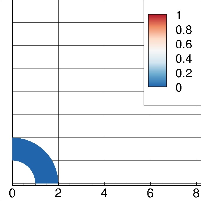
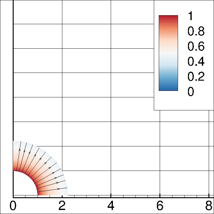
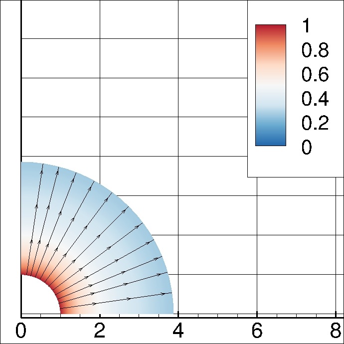
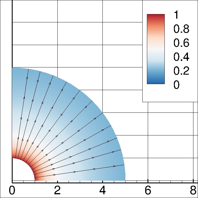
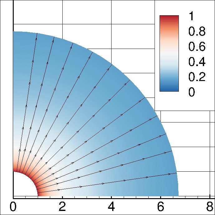
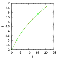
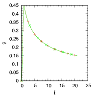
The solid membrane is stretched by more than a factor of 3. For the membrane displacement (Fig. 3) and velocity (Fig. 4) the numerical result is in perfect agreement with the analytical solution derived in Sec. 3.1; see Eqs. (39) & (40).
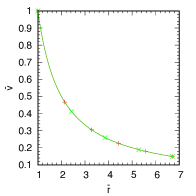
For the pressure shown in Fig. 5 we observe deviations from the analytical result (43) during the transient part and again nearly perfect agreement at the final simulation time.
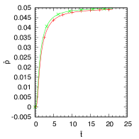
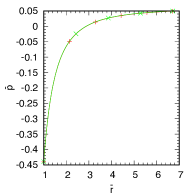
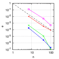
The numerical results improve for a higher mesh resolution. The finite element discretization and its implementation shows quadratic convergence behavior as expected, see Fig. 3b.
5.2 Rolling droplet
The second example simulates rolling contact of a liquid droplet on an inclined substrate considering a low Reynolds number and a contact angle of 180∘.
As we expect the motion to come close to the spinning solution of Sec. 3.2, a purely Lagrangian FE description is chosen ().
This also allows to use a classical contact description between droplet and substrate.
There is earlier computational work on rolling droplets (Rasool et al.,, 2012; Li et al.,, 2013; Thampi et al.,, 2013; Wind-Willassen and Sørensen,, 2014).
But it is either 2D, or non-FE.
So the present study seems to be the first 3D FE simulation of rolling droplets.
Novel is also the way contact is treated here – by using a computational contact algorithm with an active-set strategy.
Within that, a no-slip (sticking) condition is assumed on the contact surface, i.e. (31).
If slip occurs, a stick-slip algorithm is needed for the droplet (Sauer,, 2016).
The droplet setup considers similar parameters as in Sauer, (2016): An initially spherical droplet with radius and volume is considered under gravity loading, such that . For water at room temperature, with kg/m3, m/s2 and mN/m, this corresponds to a droplet with mm and l. The droplet surface has no additional mass, and so . For further normalization we choose and , so that ms, mN and Pa. A high fluid viscosity is chosen, i.e. Ns/m2, such that the Reynolds number becomes very small. A suitable definition for the Reynolds number of a rolling droplet is
| (108) |
where is the diameter of the contact surface and is the mean droplet velocity. The penalty parameter for sticking according to contact model (33) is taken as , where characterizes the FE resolution according to Tab. 2.
| fluid elements | membrane elements | nodes | dofs | |
|---|---|---|---|---|
| 2 | 128 | 48 | 1,241 | 4,964 |
| 4 | 832 | 192 | 7,407 | 29,628 |
| 8 | 6,656 | 768 | 56,157 | 224,628 |
| 16 | 53,248 | 3,072 | 437,433 | 1,749,732 |
Quadratic Lagrange elements are used.
The computational runtime per time step (accounting for residual and tangent matrix assembly, contact computation and Newton-Raphson iteration) is about 1 min. for , 20 mins. for and 100 mins. for .
Initially the droplet is at rest.
Rolling motion is then induced by inclining the substrate considering the time-varying inclination angle
| (109) |
with , , and the two cases:
1. with , and
2. with .
Fig. 6 shows the finite element results for the mean droplet velocity for the two cases.171717The mean droplet velocity is determined by computing the volume average of the fluid velocity and then taking its component parallel to the substrate surface.
As seen the FE results converge upon mesh refinement. The figure also shows that steady rolling motion is attained at about for , while it is attained almost instantaneously for (i.e. at ). The instantaneous response of on , for low , can be also seen from the –plot in Fig. 7.
Both branches (for increasing and decreasing , respectively) are almost identical.
For on the other hand, the two branches are different.
For further illustration, Fig. 8 shows the droplet deformation and velocity field during rolling.
The deformation is considerable and should not be neglected, as has been done in earlier work (Rasool et al.,, 2012, 2013).
The figure also shows how the contact surface changes.
Initially the contact surface is circular with a diameter of .
During steady rolling the diameter in rolling direction reduces to .
Since , the Reynolds number thus becomes according to (108).
Fig. 8 clearly shows that the advancing and receding droplet halves are not symmetric during rolling.
This can also be seen from the pressure distribution shown in Fig. 9.
The fluid pressure is largest at the advancing front of the contact surface.
Since the contact surface is flat, the fluid pressure is equal to the contact pressure.
Close inspection shows that the pressure is oscillatory in the vicinity of the contact line .
Those oscillations do not converge with mesh refinement, as the velocity field does.
So it seems that the pressure stabilization scheme, described in Sec. 2.1.4, is not sufficient to handle the contact boundary of a rolling droplet, even though the static droplet (at and ) poses no problem.
The problem may be related to the discontinuity of the contact pressure: it jumps to zero at the contact boundary.
The way the fluid velocity, fluid pressure and contact pressure are interpolated (quadratic Lagrange interpolation is used here) seem incompatible.
It seems that this problem has not yet been addressed in the literature.
Further study is required on the topic.
Perhaps -continuous interpolation, such as is provided by NURBS, would help.
We note that for , pressure oscillations also appear, but they are less pronounced.
To remove the pressure oscillations, Gaussian smoothing can be used for post-processing.
Selecting the variance of the Gaussian distribution as , i.e. on the order of the nodal distance, gives non-oscillatory pressures; see Fig. 10.
The smoothed pressure converges with mesh refinement.
The pressure distribution shows that the advancing contact surface carries most of the droplet weight (component ).
Component is equilibrated by a tangential sticking force.
The moment caused by these external forces is equilibrated by the internal moment of the fluid stress.
The last plot shows the vorticity (i.e. spin) component (along the axis of rotation ) and the dissipation during rolling; see Fig. 11.
Also here smoothing is used. According to Sec. 3.2 the vorticity of a spinning sphere is a constant vector with magnitude 2. In contrast, the vorticity of a rolling droplet is non-constant: A maximum is attained at the contact boundary and a minimum occurs on the contact surface. Although, away from the contact surface, the vorticity approaches a constant. The behavior is similar for the dissipation: Away from the contact surface, the dissipation is zero and thus agrees with the spinning sphere solution. Non-zero dissipation, associated with shear flow, occurs in the vicinity of the contact surface, with a maximum occurring at the advancing contact front. For longer rolling droplets, or for higher , the shear flow becomes more pronounced, such that an ALE formulation is needed for the mesh. On the free surface (which is tracked explicitly within the present scheme) such a formulation needs to be Lagrangian in the normal direction but Eulerian in-plane. The formulation of such an ALE scheme is outside the present scope.
5.3 Flapping flag
The third example simulates the flapping motion of a flag. The problem setup of this example is shown in Fig. 12.
The flag is modeled as a flexible sheet that is supported on the left hand side. It is excited by a uniform inflow with velocity . The length scale , the fluid density and the time scale are used to normalize the problem. The remaining parameters are chosen according to Tab. 3.
| parameter | normalized value |
|---|---|
| inflow velocity | |
| density of the fluid | |
| viscosity of the fluid | |
| density of the flag | |
| shear stiffness of the flag | |
| bending stiffness of the flag |
Considering m, s and kg/m3, the fluid parameters become and Ns/m2, which correspond to the values of air at sea level and C, while the flag parameters become kg/m2, N/m and Nm according to Sec. 4.3.181818Following Sec. 4.3, the bending stiffness needs to be normalized by , where . The Reynolds number of the problem is
| (110) |
where is the chord length of the flag.
For and the considered and follows .
At this and density ratio191919The density ratio , as defined in Shelley and Zhang, (2011), is 1/3 here., the flag motion can be expected to be chaotic according to the phase diagram of Connell and Yue, (2007).
The flapping flag example is a good test case since the flag motion and the surrounding flow field can become very complex, as the experimental data reported in Shelley and Zhang, (2011) show.
There have been recent 3D simulations that study the problem in detail (Hoffman et al.,, 2011; Banerjee et al.,, 2015; Gilmanov et al.,, 2015; de Tullio and Pascazio,, 2016).
In some of those works immersed boundary methods are used instead of ALE.
Such methods are advantageous for very large flag motions that may even involve self-contact.
In contrast to earlier work, the flag is discretized here with -continuous isogeometric shell elements.
Their formulation is the same as the one of Eq. (90) with the only exception that is extended by the internal bending moments according to the formulation of Duong et al., (2017) using the Canham bending model.
A shell formulation is used in order to regularize the system with bending stiffness.
A low stiffness value is used such that the structure remains very flexible.
Below a certain threshold value of , the flapping behavior becomes independent of as is shown later.
The fluid domain is discretized with quadratic 3D NURBS elements, while
the flag is discretized with quadratic 2D NURBS elements.
The number of nodes and dofs resulting from this discretization202020The number of nodes is ; the number of dofs is , due to the double pressure nodes on the flag surface. are listed in Tab. 4.
| fluid elements | membrane elements | nodes | dofs | |
|---|---|---|---|---|
| 2 | 512 | 24 | 1,680 | 6,744 |
| 4 | 4096 | 96 | 7,920 | 31,776 |
| 8 | 32,768 | 384 | 46,512 | 186,432 |
On the surface of the flag, double pressure dofs are used to account for pressure jumps as described in Sec. 4.1.4.
The time step is taken as .
The computational runtime per time step is about 3 mins. for and 25 mins. for .
Fig. 13 shows the flag deformation at selected time steps.
Those are snap-shots of the supplementary movie file flag v.mpg. As expected, the structure performs flag-typical oscillations along its length. Close inspection shows that the flag motion also varies in vertical direction. The pressure field around the flag is shown in Fig. 14.
The figure also shows the mesh motion around the flag.
It is based on the interpolation scheme given in App. D.
For the chosen parameters, the flapping behavior is still (quite) periodic, as Fig. 15 shows.
The period of the main oscillation is 5.60 s.
Apart from the main oscillations, there are also fine scale oscillations, as Fig. 15b shows.
Fig. 15 also shows that the simulation results converge with mesh refinement.
For the first 20 seconds, mesh already gives quite good results.
The model parameters of Tab. 3 affect the flapping behavior of the flag.
The influence of has been discussed in detail in earlier work, e.g. see Shelley and Zhang, (2011), so the following discussion focuses on the membrane parameters. Three aspects are noteworthy:
1. For sufficiently low , the flapping behavior (for given ) remains unchanged, i.e. it becomes independent of .
According to Fig. 16a this occurs below .
Below that , the flag is effectively a membrane without bending stiffness, and is only helpful for regularizing the numerical solution.
2. Increasing leads to increased fine scale oscillations, as Fig. 16b shows.
Since controls the in-plane stiffness of the flag, those oscillations can be associated with longitudinal vibrations of the flag.
3. Increasing the ratio between fluid and membrane density does not degrade the computational robustness of the proposed monolithic scheme:
Fig. 17 shows the flapping behavior for various density ratios.
For ( here), the nodal FE forces due to fluid and membrane inertia are equal in the limit (since const. across the element thickness). For all the considered density ratios, the Newton-Raphson iteration at each time step converges to a normalized energy residual of within an average of six iterations. The density ratio therefore does not have a negative affect on the computational stability or the conditioning of the system. This is different to partitioned FSI schemes, which have been shown to suffer from a loss of robustness as the inertia forces of the flow become comparable or larger than those of the structure (Le Tallec and Mouro,, 2001; Causin et al.,, 2005). The reason lies in the strong effect of the fluid on the structure for high fluid densities that is not well captured by weakly coupled partitioned schemes or requires many staggering steps in strongly coupled partitioned schemes. The extreme case of this effect occurs when , which was considered in the droplet example of Sec. 5.2. Also in this case no stability issues were encountered in all simulations.
6 Conclusion
A unified FSI formulation is presented that is suitable for solid, liquid and mixed membranes.
At free liquid surfaces, sticking contact can be accounted for.
The fluid flow and the structure are discretized with finite elements using a stabilized fluid formulation and a surface-based membrane formulation.
A conforming interface discretization is used between fluid and membrane, which leads to a simple monolithic coupling formulation.
On membrane surfaces surrounded by fluid on both sides, double pressure nodes are required.
The temporal discretization is based on the generalized- scheme.
Two analytical and three numerical examples are presented in order to illustrate and verify the proposed formulation.
They consider fluid flow at low and high Reynolds numbers exhibiting strong FSI coupling.
The proposed formulation is very general and thus suitable as a basis for further research.
In order to increase efficiency, the formulation can be extended to boundary elements (for low ) or turbulence models (for high ).
Under current study is the use of enriched finite element discretizations (Harmel et al.,, 2017) that are suitable to efficiently capture boundary layers (Rasool et al.,, 2016).
Another extension of the present formulation is to re-examine the pressure stabilization scheme at contact boundaries.
This would be especially important in the presence of sharp contact angles.
Such a formulation would then allow for a detailed flow analysis of droplets on rough surfaces.
Acknowledgements
The authors are grateful to the German Research Foundation (DFG) for supporting this research under grants GSC 111 and SA1822/3-2. The authors also wish to thank Maximilian Harmel and Raheel Rasool for proofreading the manuscript.
Appendix A Uniform membrane stretch
Appendix B FE tangent matrices for the time-continuous system
B.1 Fluid element
In order to evaluate the tangent matrix of the finite element force vector defined in (70), we require
| (114) |
which can be written as with
| (115) |
Therefore
| (116) |
Based on this, we find the tangent matrices of the fluid forces defined in (72)-(74)
| (117) |
As seen, a major source of complexity are the stabilization terms and .
B.2 Membrane element
Linearizing the membrane forces in (91) w.r.t. and yields the mass matrix
| (118) |
and the stiffness matrix
| (119) |
The first term of follows from Sauer et al., (2014) as
| (120) |
with
| (121) |
and
| (122) |
Here,
| (123) |
for model (29) and
| (124) |
for model (30), see Sauer et al., (2014) and Sauer and Duong, (2017). Inserting these into (120), yields the simpler expression
| (125) |
for model (29) and
| (126) |
for model (30). Here is the identity tensor on surface . With this, can be further simplified, in particular for model (30), see Sauer, (2016).
The second term of depends on the contact description. Here, sticking contact is considered with a rigid substrate using the penalty regularization of Eq. (33). For this case, we have
| (127) |
with
| (128) |
The front term of follows directly from Eqs. (33) and (85), while the rear term is derived in Sauer and De Lorenzis, (2015).
Appendix C FE tangent matrices for the time-discrete system
C.1 Fluid element
C.2 Membrane element
Appendix D Mesh motion for the flapping flag example
For the flapping flag example in Sec. 5.3, the mesh velocity (with Cartesian components ) at FE node (i.e. control point) is defined by the linear interpolation
| (134) |
for the inflow direction, and
| (135) |
for the other directions (). Here are the components of , is the distance of from the flag surface, and is the current flag velocity at the initially nearest membrane gridpoint . Note that is smooth at since approaches 0 smoothly as .
References
- Banerjee et al., (2015) Banerjee, S., Connell, B. S. H., and Yue, D. K. P. (2015). Three-dimensional effects on flag flapping dynamics. J. Fluid Mech., 783:103–136.
- Barett et al., (2015) Barett, J. W., Garcke, H., and Nürnberg, R. (2015). Numerical computations of the dynamics of fluidic membranes and vesicles. Phys. Rev. E., 92:052704.
- Bazilevs and Takizawa, (2016) Bazilevs, Y. and Takizawa, K., editors (2016). Advances in Computational Fluid-Structure Interaction and Flow Simulation. Springer, Berlin, Heidelberg.
- Bazilevs et al., (2013) Bazilevs, Y., Takizawa, K., and Tezduyar, T. E. (2013). Computational Fluid-Structure Interaction: Methods and Applications. John Wiley & Sons, Hoboken.
- Bletzinger et al., (2006) Bletzinger, K.-U., Wüchner, and Kupzok, A. (2006). Algorithmic treatment of shells and free form-membranes in FSI. In Bungartz, H. and Schäfer, M., editors, Fluid-Structure Interaction. Lecture Notes in Computational Science and Engineering, vol. 53, pages 336–355, Berlin, Heidelberg. Springer.
- Brooks and Hughes, (1982) Brooks, A. N. and Hughes, T. J. R. (1982). Streamline upwind/Petrov-Galerkin formulations for convection dominated flows with particular emphasis on the incompressible Navier-Stokes equations. Adv. Appl. Mech., 32:199–259.
- Causin et al., (2005) Causin, P., Gerbeau, J. F., and Nobile, F. (2005). Added-mass effect in the design of partitioned algorithms for fluid-structure problems. Comput. Methods Appl. Mech. Engrg., 194:4506–4527.
- Chung and Hulbert, (1993) Chung, J. H. and Hulbert, G. M. (1993). A time integration algorithm for structural dynamics with improved numerical dissipation: the generalized- method. J. Appl. Mech., 60:371–375.
- Connell and Yue, (2007) Connell, B. S. H. and Yue, D. K. P. (2007). Flapping dynamics of a flag in a uniform stream. J. Fluid. Mech., 581:33–67.
- Cottrell et al., (2009) Cottrell, J. A., Hughes, T. J. R., and Bazilevs, Y. (2009). Isogeometric Analysis. Wiley, Hoboken.
- Cristini and Tan, (2004) Cristini, V. and Tan, Y.-C. (2004). Theory and numerical simulation of droplet dynamics in complex flows – a review. Lab Chip, 4:257–264.
- de Tullio and Pascazio, (2016) de Tullio, M. D. and Pascazio, C. (2016). A moving-least-squares immersed boundary method for simulating the fluid-structure interaction of elastic bodies with arbitrary thickness. J. Comput. Phys., 325:201–225.
- Dhatt and Touzot, (1984) Dhatt, G. and Touzot, G. (1984). The Finite Element Method Displayed. Wiley, Hoboken.
- Donea and Huerta, (2003) Donea, J. and Huerta, A. (2003). Finite Element Methods for Flow Problems. Wiley, Hoboken.
- Dowell and Hall, (2001) Dowell, E. H. and Hall, K. C. (2001). Modeling of fluid-structure interaction. Ann. Rev. Fluid Mech., 33:445–490.
- Duong et al., (2017) Duong, T. X., Roohbakhshan, F., and Sauer, R. A. (2017). A new rotation-free isogeometric thin shell formulation and a corresponding continuity constraint for patch boundaries. Comput. Methods Appl. Mech. Engrg., 316:43–83.
- Franci et al., (2016) Franci, A., Oñate, E., and Carbonell, J. M. (2016). Unified Lagrangian formulation for solid and fluid mechanics and FSI problems. Comput. Methods Appl. Mech. Engrg., 298:520–547.
- Gilmanov et al., (2015) Gilmanov, A., Le, T. B., and Sotiropoulos, F. (2015). A numerical approach for simulating fluid structure interaction of flexible thin shells undergoing arbitrarily large deformations in complex domains. J. Comput. Phys., 300:814–843.
- Ha et al., (2017) Ha, S. T., Ngo, L. C., Saeed, M., Jeon, B. J., and Choi, H. (2017). A comparative study between partitioned and monolithic methods for the problems with 3D fluid-structure interaction of blood vessels. J. Mech. Sci. Tech., 31(1):281–287.
- Harmel et al., (2017) Harmel, M., Sauer, R. A., and Bommes, D. (2017). Volumetric mesh generation from T-spline surface representations. Comput. Aid. Des., 82:13–28.
- Heil et al., (2008) Heil, M., Hazel, A. L., and Boyle, J. (2008). Solvers for large-displacement fluid-structure interaction problems: Segregated versus monolithic approaches. Comput. Mech., 43:91–101.
- Heltai et al., (2017) Heltai, L., Kiendl, J., DeSimone, A., and Reali, A. (2017). A natural framework for isogeometric fluid-structure interaction based on BEM-shell coupling. Comput. Methods Appl. Mech. Engrg., 316:522–546.
- Hoffman et al., (2011) Hoffman, J., Jansson, J., and Stöckli, M. (2011). Unified continuum modeling of fluid-structure interaction. Math. Mod. Meth. Appl. Sci., 21(3):491–513.
- Hughes et al., (1986) Hughes, T. J. R., Franca, L. P., and Balestra, M. (1986). A new finite element formulation for computational fluid dynamics: V. Circumventing the Babuška-Brezzi condition: A stable Petrov-Galerkin formulation of the Stokes problem accommodating equal-order interpolations. Comput. Methods Appl. Mech. Engrg., 59(1):85–99.
- Idelsohn et al., (2004) Idelsohn, S. R., Oñate, E., and Del Pin, F. (2004). The particle finite element method: a powerful tool to solve incompressible flows with free-surfaces and breaking waves. Int. J. Num. Meth. Engrg., 61:964–989.
- Idelsohn et al., (2006) Idelsohn, S. R., Oñate, E., Del Pin, F., and Calvo, N. (2006). Fluid-structure interaction using the particle finite element method. Comput. Methods Appl. Mech. Engrg., 195:2100–2123.
- Jansen et al., (2000) Jansen, K. E., Whiting, C. H., and Hulbert, G. M. (2000). A generalized- method for integrating the filtered Navier-Stokes equations with a stabilized finite element method. Comput. Methods Appl. Mech. Engrg., 190:305–319.
- Karagiozis et al., (2011) Karagiozis, K., Kamakoti, R., Cirak, F., and Pantano, C. (2011). A computational study of supersonic disk-gap-band parachutes using large-eddy simulation coupled to a structural membrane. J. Fluids Struc., 27:175–192.
- Kloeppel and Wall, (2011) Kloeppel, T. and Wall, W. A. (2011). A novel two-layer, coupled finite element approach for modeling the nonlinear elastic and viscoelastic behavior of human erythrocytes. Biomech. Model. Mechanobiol., 10(4):445–459.
- Küttler et al., (2010) Küttler, U., Gee, M., Förster, C., Comerford, A., and Wall, W. A. (2010). Coupling strategies for biomedical fluid-structure interaction problems. Int. J. Numer. Meth. Biomed. Engng., 26:305–321.
- Laursen, (2002) Laursen, T. A. (2002). Computational Contact and Impact Mechanics: Fundamentals of modeling interfacial phenomena in nonlinear finite element analysis. Springer, Berlin, Heidelberg.
- Le et al., (2009) Le, D. V., White, J., Peraire, J., Lim, K. M., and Khoo, B. C. (2009). An implicit immersed boundary method for three-dimensional fluid–membrane interactions. J. Comput. Phys., 228:8427–8445.
- Le Tallec and Mouro, (2001) Le Tallec, P. and Mouro, J. (2001). Fluid structure interaction with large structural displacements. Comput. Methods Appl. Mech. Engrg., 190(24-25):3039–3067.
- Li et al., (2013) Li, Z., Hu, G.-H., Wang, Z.-L., Ma, Y.-B., and Zhou, Z.-W. (2013). Three dimensional flow structures in a moving droplet on substrate: A dissipative particle dynamics study. Phys. Fluids, 25:072103.
- Liang et al., (1997) Liang, S. J., Neitzel, G. P., and Aidun, C. K. (1997). Finite element computations for unsteady fluid and elastic membrane interaction problems. Int. J. Num. Meth. Fluids, 24:1091–1110.
- Mayer et al., (2010) Mayer, U. M., Popp, A., Gerstenberger, A., and Wall, W. A. (2010). 3D fluid-structure-contact interaction based on a combined XFEM FSI and dual mortar contact approach. Comput. Mech., 46:53–67.
- Montefuscolo et al., (2014) Montefuscolo, F., Sousa, F. S., and Buscaglia, G. C. (2014). High-order ALE schemes for incompressible capillary flows. J. Comput. Phys., 278:133–147.
- Ohayon, (2004) Ohayon, R. (2004). Fluid-structure interaction problems. In Stein, E., de Borst, R., and Hughes, T. J. R., editors, Encyclopedia of Computational Mechanics. Vol. 2: Solids and Structures. Chapter 21, Hoboken. Wiley.
- Peskin, (2003) Peskin, C. S. (2003). The immersed boundary method. Acta Numerica, 11:479–517.
- Rangarajan and Gao, (2015) Rangarajan, R. and Gao, H. (2015). A finite element method to compute three-dimensional equilibrium configurations of fluid membranes: Optimal parameterization, variational formulation and applications. J. Comput. Phys., 297:266–294.
- Rasool et al., (2016) Rasool, R., Corbett, C. J., and Sauer, R. A. (2016). A strategy to interface isogeometric analysis with Lagrangian finite elements – Application to incompressible flow problems. Computers & Fluids, 127:182–193.
- Rasool et al., (2013) Rasool, R., Osman, M., and Sauer, R. A. (2013). Computational modeling of liquid droplets moving on rough surfaces. Proc. Appl. Math. Mech., 13:233–234.
- Rasool et al., (2012) Rasool, R., Sauer, R. A., and Osman, M. (2012). Internal flow analysis for slow moving small droplets in contact with hydrophobic surfaces. Proc. Appl. Math. Mech., 12:489–490.
- Sahu et al., (2017) Sahu, A., Sauer, R. A., and Mandadapu, K. K. (2017). Irreversible thermodynamics of curved lipid membranes. Phys. Rev. E, 96:042409.
- Saksono and Perić, (2006) Saksono, P. H. and Perić, D. (2006). On finite element modelling of surface tension: Variational formulation and applications - Part II: Dynamic problems. Comp. Mech., 38(3):251–263.
- Sauer, (2014) Sauer, R. A. (2014). Stabilized finite element formulations for liquid membranes and their application to droplet contact. Int. J. Numer. Meth. Fluids, 75(7):519–545.
- Sauer, (2016) Sauer, R. A. (2016). A frictional sliding algorithm for liquid droplets. Comput. Mech., 58(6):937–956.
- Sauer and De Lorenzis, (2015) Sauer, R. A. and De Lorenzis, L. (2015). An unbiased computational contact formulation for 3D friction. Int. J. Numer. Meth. Engrg., 101(4):251–280.
- Sauer and Duong, (2017) Sauer, R. A. and Duong, T. X. (2017). On the theoretical foundations of solid and liquid shells. Math. Mech. Solids, 22(3):343–371.
- Sauer et al., (2014) Sauer, R. A., Duong, T. X., and Corbett, C. J. (2014). A computational formulation for constrained solid and liquid membranes considering isogeometric finite elements. Comput. Methods Appl. Mech. Engrg., 271:48–68.
- Sauer et al., (2017) Sauer, R. A., Duong, T. X., Mandadapu, K. K., and Steigmann, D. J. (2017). A stabilized finite element formulation for liquid shells and its application to lipid bilayers. J. Comput. Phys., 330:436–466.
- Seifert, (1997) Seifert, U. (1997). Configurations of fluid membranes and vesicles. Advances in Physics, 46:13–137.
- Shakib, (1988) Shakib, F. (1988). Finite element analysis of the incompressible Euler and Navier-Stokes equations. PhD thesis, Stanford University, Stanford, USA.
- Shelley and Zhang, (2011) Shelley, M. J. and Zhang, J. (2011). Flapping and bending bodies interacting with fluid flows. Annu. Rev. Fluid Mech., 43:449–465.
- Takizawa and Tezduyar, (2012) Takizawa, K. and Tezduyar, T. E. (2012). Computational Methods for Parachute Fluid–Structure Interactions. Arch. Comput. Meth. Eng., 19:125–169.
- Tezduyar, (1992) Tezduyar, T. E. (1992). Stabilized finite element formulations for incompressible flow computations. Advances in Applied Mechanics, 28:1–44.
- Tezduyar and Sathe, (2007) Tezduyar, T. E. and Sathe, S. (2007). Modelling of fluid–structure interactions with the space–time finite elements: Solution techniques. Int. J. Num. Meth. Fluids, 54:855–900.
- Tezduyar et al., (2006) Tezduyar, T. E., Sathe, S., Stein, K., and Aureli, L. (2006). Modeling of fluid-structure interactions with the space-time techniques. In Bungartz, H. and Schäfer, M., editors, Fluid-Structure Interaction. Lecture Notes in Computational Science and Engineering, vol. 53, pages 50–81, Berlin, Heidelberg. Springer.
- Thampi et al., (2013) Thampi, S. P., Adhikari, R., and Govindarajan, R. (2013). Do liquid drops roll or slide on inclined surfaces? Langmuir, 29(10):3339–3346.
- van Loon et al., (2007) van Loon, R., Anderson, P. D., van de Vosse, F. N., and Sherwin, S. J. (2007). Comparison of various fluid–structure interaction methods for deformable bodies. Comp. Struct., 85:833–843.
- van Opstal et al., (2015) van Opstal, T. M., van Brummelen, E. H., and van Zwieten, G. J. (2015). A finite-element/boundary-element method for three-dimensional, large-displacement fluid–structure-interaction. Comput. Methods Appl. Mech. Engrg., 284:637–663.
- Walkley et al., (2005) Walkley, M. A., Gaskell, P. H., Jimack, P. K., Kelmanson, M. A., and Summers, J. L. (2005). Finite element simulation of three-dimensional free-surface flow problems with dynamic contact lines. Int. J. Num. Meth. Fluids, 47:1353–1359.
- Wind-Willassen and Sørensen, (2014) Wind-Willassen, Ø. and Sørensen, M. P. (2014). A finite-element method model for droplets moving down a hydrophobic surface. Eur. Phys. J. E, 37:65.
- Wriggers, (2006) Wriggers, P. (2006). Computational Contact Mechanics. Springer, Berlin, Heidelberg, 2 edition.
- Yang et al., (2016) Yang, P., Xiang, J., Fang, F., Pavlidis, D., Latham, J. P., and Pain, C. C. (2016). Modelling of fluid–structure interaction with multiphase viscous flows using an immersed-body method. J. Comput. Phys., 321:571–592.