Intervention On Default Contagion Under Partial Information

Abstract.

We model the default contagion process in a large heterogeneous financial network under the interventions of a regulator (a central bank) with only partial information which is a more realistic setting than most current literature. We provide the analytical results for the asymptotic optimal intervention policies and the asymptotic magnitude of default contagion in terms of the network characteristics. We extend the results of Amini et al. (2013) to incorporate interventions and the model of Amini et al. (2015, 2017) to heterogeneous networks with a given degree sequence and arbitrary initial equity levels. The insights from the results are that the optimal intervention policy is "monotonic" in terms of the intervention cost, the closeness to invulnerability and connectivity. Moreover, we should keep intervening on a bank once we have intervened on it. Our simulation results show a good agreement with the theoretical results.

Important formulations and programs

Formulations and programs	Page
Asymptotic control problem (ACP)	ACP
Optimal control problem (OCP)	OCP
Optimization problem (OP)	OP

Important index sets

$\Gamma\coloneqq\{(i,j,c,l):0\leq i,0\leq j,0\leq l<c\leq i\text{ or }c=i+1,l=i\},$

$\Phi\coloneqq\{(i,j,c,c-1):0\leq i,0\leq j,1\leq c\leq i\}.$

For some integer $M^{\epsilon}$,

$\Gamma^{\epsilon}\coloneqq\{(i,j,c,l):i\lor j<M^{\epsilon},0\leq l<c\leq i\text{ or }c=i+1,l=i\},$

$\Phi^{\epsilon}\coloneqq\{(i,j,c,c-1):i\lor j<M^{\epsilon},0\leq c\leq i\}.$

Part I Introduction

1. Introduction

The systemic risk defined as the large scale defaults of financial institutions in a financial network has been drawing more and more interest of regulators and researchers in the recent decade, especially after the Asian financial crsises in the late 1990’s and the more recent economic recession in 2008 and 2009. In a modern financial system, financial institutions (hereafter, banks), connected through lending and borrowing relations constitute a financial network. Due to the intricate nature of the interconnectedness, the default of some banks in the network may lead to losses of creditor banks through interbank connections, which may in turn results in losses of their creditors. This process goes on and creates risk at the system level.

We model the contagion process in a financial network under a short term illiquidity risk. In this setting no banks would want to lend new loans to other banks meanwhile they are still obliged to pay back their current loans which are due in the time frame of the model. So we fix the in and out degrees of banks in the network, and set up a probability space under which the financial network is generated by a uniform matching of the in and out degrees (a configuration model). A directed link in this model represents one unit of loan. In the following we may use “bank” and “node” interchangeably.

Before an external shock to the system, each node has a positive equity level, which indicates the number of lost loans a node can withstand due to the default of its debtors before it defaults. In other words, it is the “distance to default”. After an external shock, some nodes in the system default initially and we set their equity level to zero. We consider the default contagion in the following way. When a node defaults, it defaults on all of its loan liabilities. We assume a zero recovery rate of the loan, i.e. the creditor receives zero value from the loan, which is the most realistic assumption for short term default as suggested in Cont et al. (2010a) and Amini et al. (2013). But there is a time span between a node’s default and the time its creditor records the loan as a loss (by writing down the loan from its balance sheet). We model this time span by independently, identically exponentially distributed random variables. After the affected node records the lost loan, it may request the regulator for interventions. This corresponds to the central bank’s provision of short term liquidity to banks, including the traditional discount window, the Term Auction Facility (TAF), etc, as well as the government’s interventions by bailing out the stressed banks. If the regulator decides to intervene by infusing one unit of equity, the equity level of the affected node will stay the same, otherwise its equity level will decrease by one. Once the equity level reaches zero, the node defaults. We assume that the once a bank has defaulted it cannot become liquid again within the time horizon of the model because it is very unlikely for a bank that has declared default to gain enough credits in a short term as considered in the model. During the contagion process, the regulator knows the default set (the set of defaulted nodes) and the set of revealed out links from the default set, but other out links from the default set are hidden until the affected nodes record the defaulted loans.

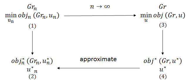
Figure 1.1. The methodology: approximation of the finite network with the infinite network

Our methodology is illustrated in 1.1. The regulator’s goal is to minimize the number of final defaulted nodes with the minimum number of interventions, so we obtain a stochastic control problem $\min_{u_{n}}\text{obj}_{n}(Gr{}_{n},u_{n})$ where the objective function depends on the graph $Gr_{n}$ and the intervention policy $u_{n}$, shown in (1). We aim to solve it for the optimal intervention policy $u_{n}^{*}$ and thus obtain the optimal objective function value $\text{obj}_{n}(Gr_{n},u_{n}^{*})$, shown in (2). However, solving the problem with the usual dynamic programming approach will incur intractability problem because of the fast expansion of the state space as in Amini et al. (2015, 2017), not to mention the heterogeneous network in our setting. We take an alternative approach based on the fact that under some regularity conditions, the objective function converges as $n\rightarrow\infty$. We solve the asymptotic optimal control problem $\min_{u}\text{obj}(Gr,u)$ in (3) where obj, $Gr$ and $u$ are the limit forms of $\text{obj}_{n}$, $Gr_{n}$ and $u_{n}$, respectively, and obtain the optimal policy $u^{*}$ and the objective function $\text{obj}(Gr,u^{*})$ in (4), then we will be able to construct the optimal intervention policy $u_{n}^{*}$ for a finite $n$ through $u^{*}$ and approximate $\text{obj}_{n}(Gr_{n},u_{n}^{*})$ with $\text{obj}(Gr,u^{*})$. Our results of the numerical experiments validate the approximation for networks with sizes close to the real financial networks.

2. Relations to previous literature

To understand the systemic risk the existing literature tries to relate the systemic propagation of financial stress to various features of the financial network and the banks within it, including the degree of connectivity, the equity levels and so on. There are mainly two types of literature: empirical and theoretical. The empirical studies conduct statistical analysis on the interbank markets using data on interbank lending and borrowing as far as they are available and provide an overview of the structural characteristics of the interbank network in different countries (Furfine (2003); Cont, Moussa, and Santos (2010b); Boss and Elsinger (2004)). The theoretical studies model the financial network with network models but differ in their assumptions of the network structure and approaches, some focus on “stylized” networks whose structures are hypothetical (Allen and Gale (2000); May and Arinaminpathy (2010); Haldane and May (2011); Gai et al. (2011)) while others reply on simulations (Nier, Yang, Yorulmazer, and Alentorn (2007); Cont, Moussa, and Santos (2010b)). Among them, Amini et al. (2013) and Eisenberg and Noe (2001) propose random network models that allow more realistic, heterogeneous structures. From the regulatory perspective, there are mainly two shortcomings in the studies. While it is important to understand the dependence of systemic risk on network features, it is still unclear in the system risk literature on how the regulator (such as the central bank) can do optimally to intervene on the contagion of financial stress in the network. Moreover, the majority of studies assume the regulator has complete information of the network which does not align with the reality, as for example pointed out by Hurd (2015): “Interbank exposure data are never publicly available, and in many countries nonexistent even for central regulators”. Although there are some attempts for considering partial information in a financial network (Song and van der Schaar (2015); Battiston et al. (2012); Amini et al. (2015)), they either focus on simplified networks or lack analytical results of the regulator’s optimal strategies.

In particular, our work is an extension of the papers Amini et al. (2013), Amini et al. (2015) and Amini et al. (2017). Amini et al. (2013) model a financial network as a weighted directed graph where the weight represents the amount of loan liabilities between two banks. Then they show that under some conditions a random weighted directed graph has the same law as a unweighted directed graph with a default threshold on each node and propose a sequential construction algorithm to model the development of the default set. The default contagion model in our work extends the construction algorithm to incorporate interventions. Thus if there are no interventions, the asymptotic fraction of defaults will be the same as in Amini et al. (2013).

Amini et al. (2015, 2017) consider a stylized core-periphery financial network where the core consists of identical nodes, i.e. each core node having the same in and out degrees and initial equity level if it is liquid or zero otherwise, and each periphery node having in degree of one and one initial equity. We consider a heterogeneous network where the nodes have arbitrary in and out degrees and initial equity levels. We adopted the dynamics of their model which constructs the default set with interventions through a configuration model due to the fact that the configuration model can be adapted to modeling the contagion process as described in van der Hofstad (2014).

Amini et al. (2015) solve a stochastic control problem for a finite network in which the regulator seeks to maximize under budget constraints the value of the financial system defined as the total number of projects. Amini et al. (2017) also deals with a finite network with the objective to minimize under some budget the expected loss at the end of the cascade. They take the pair (remaining equity level of banks, the number of interventions on banks with the same remaining equity) as the system state and apply the dynamic programming approach. The limitation of the approach is that the state space expands very fast as the type of banks and the total number of interventions increase, rendering the problem intractable. In Amini et al. (2017) they present an example of a network of $20$ core banks, each having initial equity level $3$ and $20$ periphery banks and total $12$ interventions, the state space is about $10^{9}$. Motivated by the intention to overcome the limitations, we solve an optimal control problem to approximate the solution of a stochastic control problem in which the regulator seeks to minimize the number of final defaults with the minimum number of interventions, and give analytical formulations for the optimal intervention policies as well as the asymptotic number of interventions and final defaulted banks. The asymptotic results provide a good approximation to real financial networks, which are heterogeneous and have several hundreds of banks thanks to the fast convergence behavior of our results. We have run numerical experiments and validated the convergence behavior.

3. Contributions

The main contribution of our work is that we derive rigorous asymptotic results of the optimal strategy for the regulator and the fraction of final defaults for a heterogeneous network with a given degree sequence and arbitrary initial equity levels. The analytical expressions are expressed in terms of measurable features of the network. For convergence of the results we assume the network is sparse which are supported by the empirical studies of real financial networks (e.g. Furfine (1999); Bech and Atalay (2010)) and used by some theoretical studies (e.g. Amini et al. (2013)) .

The key insight of our findings of the optimal strategies is that we should only consider intervention on a bank when it is very close to default, so we never intervene on an invulnerable bank. The optimal intervention policy depends strongly on the intervention cost. The smaller intervention cost, the more interventions are implemented. Moreover, the optimal intervention policy is “monotonic” with respect to the measurable features of the network: We should not intervene on the banks with out degrees in a certain range regardless of their other features. For those banks worth interventions, the larger the sum of initial equity and accumulative interventions received, the earlier we should begin intervening if they are affected. Moreover, the time to start intervention on a node is also “monotonic” in its in and out degree. Once we begin intervening on a node we keep intervening on it every time it is affected. By comparing the fractions of final defaults under no interventions and the optimal intervention policy, we are able to quantify the improvement made by interventions in terms of the network features. This gives guidance as the maximum impact the regulator can have to offset the contagion of defaults.

The paper is organized as follows. We set up the model and introduce the stochastic control problem (SCP) in II. In III we formulate the asymptotic control problem (ACP) that gives the limit for the objective function of the SCP as the size of the network goes to infinity and present the necessary conditions for the optimal intervention policy, which lead to the main theorems. At last we show the results of the numerical experiments to validate the approximation of ACP to SCP.

Part II Model Description and Dynamics

4. Basic setup

We model a financial network with prescribed degree sequence $(d^{-}(v),d^{+}(v))_{v\in[n]}$ as an unweighted directed network $([n],\mathcal{E}_{n})$, where $[n]=\{1,\ldots,n\}$ is the set of nodes, $\mathcal{E}_{n}$ denotes the set of links, and $m=\sum_{v\in[n]}d^{-}(v)=\sum_{v\in[n]}d^{+}(v)$. We understand the prescribed degree sequence $(d^{-}(v),d^{+}(v))_{v\in[n]}$ as a set of random variables living in a probability space then we set up the following model conditioning on it. A directed link $(v,w)\in\mathcal{E}_{n}$ represents $v$ borrows a unit of loan from $w$, i.e. $v$ is obliged to repay $w$ one unit of loan. We allow multiple loans to exist between two nodes. $\mathcal{E}_{n}$ needs to satisfy that

$$d^{-}(v) =|\{(w,v):(w,v)\in\mathcal{E}_{n}\}|,$$

$$d^{+}(v) =|\{(v,w):(v,w)\in\mathcal{E}_{n}\}|,$$

where $\left|A\right|$ represents the cardinality of the set $A$. Now we set up a probability space $(G_{n,m},\mathbb{P})$ where $G_{n,m}$ is the set of networks on $n$ nodes with at most $m$ directed links. Recall $m$ is total in or out degree of the network. So the random financial network lives in this probability space and under $\mathbb{P}$ the law of the random link set $\mathcal{E}_{n}$ is determined as follows. We start with $n$ unconnected nodes and assign node $v$ with $d^{-}(v)$ in half links and $d^{+}(v)$ out half links. An in half link represents an offer of a loan and an out half link a demand for a loan. Then the $m$ in half links and $m$ out half links are matched uniformly so that the borrowers and lenders are determined. The resulting random network is called the configuration model.

Remark 4.1.

The uniform matching of the in and out half links allows us to construct the random network sequentially: at every step we can choose any out half link by any rule and choose the other in half link uniformly over all available in half links to form a directed link. This is because conditional on any set of observed matched links, the hidden matched links also follow the uniform distribution. Moreover, the conditional law of hidden matched links only depends on the number of the observed matched links, not the matching history. Additionally we can restrict the matching to out half links from the defaulted nodes so that we can model the development of the set of defaulted nodes with their revealed out links.

Then we endow a node $v\in[n]$ with its initial equity level $e_{0}^{v}\in\mathbb{N}_{0}$ which represents the number of lost loans $v$ can tolerate until $v$ defaults, so it is the “distance to default”. Next after the system receives some external shock, some nodes default and the system begins to evolve. Define time $0$ as the time right after the shock. Let $(\mathcal{G}_{k})_{0\leq k\leq m}$ be the filtration for the probability space $(G_{n,m},\mathbb{P})$ which models the arrival of new information, i.e. the revealed link at each step. Because this implies that the revealed node will have its remaining equity decrease by one, $(\mathcal{G}_{k})_{0\leq k\leq m}$ also models the default contagion at the same time. Note in the following the network with the set of revealed links evolves in the space $G_{n,m}$ as the result of the contagion process.

4.1. Initial condition

From the initial equity levels $(e_{0}^{v})_{v\in[n]}$ we can determine the initial default set $\mathcal{D}_{0}=\{v:\ e_{0}^{v}=0\}$. Let the set of hidden out links from the nodes in $\mathcal{D}_{0}$ be $Q_{0}=\{(i,j)\in\mathcal{E}_{n}:i\in\mathcal{D}_{0}\}$. All the hidden links in $Q_{0}$ are assigned a clock which rings after a random time following an independent exponential distribution with mean $1$, i.e. $\exp(1)$. Let the sigma-algebra representing the information available initially be $\mathcal{G}_{0}=\sigma\{(e_{0}^{v})_{v\in[n]}\}$. Let $c_{k}^{v}$ be the sum of initial equity and accumulative number of interventions on node $v$ and $l_{k}^{v}$ be the number of revealed in links of node $v$ at step $k$, so $c_{0}^{v}=e_{0}^{v}$, $l_{0}^{v}=0$.

4.2. Dynamics

Let $k$ be the $k$th event that a clock rings. If $Q_{k-1}$ is nonempty, let $(V_{k},W_{k})$ be a pair of random variables representing the hidden link from node $V_{k}$ to node $W_{k}$ whose clock rings first at step $k$, which means that the node $W_{k}$ records the loss of loan due to the default of $V_{k}$. We call that $(V_{k},W_{k})$ is revealed and $W_{k}$ is selected. Assume $(V_{k},W_{k})=(v,w)$. We proceed with the following steps:

• Update $\mathcal{G}_{k}=\sigma\left(\mbox{$\mathcal{G}$}_{k-1}\cup\left\{(v,w)\right\}\right)$.

• Update the number of revealed out links: $l_{k}^{w}=l_{k-1}^{w}+1$ and $l_{k}^{\eta}=l_{k-1}^{\eta}$ for $\eta\neq w$.

• Determine the intervention $\mu_{k}\in\{0,1\}$ $\mathcal{G}_{k}$ measurable at step $k$ for the selected node $w$.

• Update $c_{k}^{w}=c_{k-1}^{w}+\mu_{k}^{w}$, otherwise $c_{k}^{\eta}=c_{k-1}^{\eta}$ for $\eta\neq w$.

• Update the default set. Note that $c_{k}^{\eta}\leq l_{k}^{\eta}$ indicates that the node $\eta$ has defaulted by step $k$. If $c_{k}^{w}\leq l_{k}^{w}$ and $w\notin\mathcal{D}_{k-1}$, then $\mathcal{D}_{k}=\mathcal{D}_{k-1}\cup\{w\}$ and $Q_{k}=Q_{k-1}\backslash\{(v,w)\}\cup\{(w,\eta)\in\mathcal{E}_{n}\}$ and every newly added hidden link in $\{(w,\eta)\in\mathcal{E}_{n}\}$ is assigned a clock with law $\exp(1)$, independent of everything else. If $c_{k}^{w}>l_{k}^{w}$, $\mathcal{D}_{k}=\mathcal{D}_{k-1}$ and $Q_{k}=Q_{k-1}\backslash\{(v,w)\}$.

If $Q_{k}$ is empty, the process ends and let the process end time be $T_{n}=k$, otherwise repeat the process. Define $D_{n}$ as the number of defaulted nodes by the process end time $T_{n}$.

Lemma 4.1.

(Adapted from Lemma 3.2 in Amini et al. (2015)) For $0\leq k\leq T_{n}-1$, the selected node $W_{k+1}$ which is at the end of the revealed link $(V_{k+1},W_{k+1})$ from the set $Q_{k}$ has the probability conditional on the sigma-algebra $\mathcal{G}_{k}$ that

(4.2.1) $$\mathbb{P}(W_{k+1}=w\mid\mathcal{G}_{k})=\frac{d^{-}(w)-l_{k}^{w}}{m-k}\text{ for }w\in[n].$$

Proof.

Because $0\leq k\leq T_{n}-1$, $Q_{k}\neq\emptyset$ by definition. At step $k$ because the clocks on the hidden links follow independently and identically distributed exponential distribution which has the memoryless property, a link is chosen uniformly among all the hidden links and revealed. By 4.1, the conditional law of the identity of the selected node is given by the uniform matching to the available in half links when the network is constructed sequentially. Note in (4.2.1) the numerator $d^{-}(w)-l_{k}^{w}$ is the total number of available in half links of node $w$. Because at every step an in half link is connected and there are $k$ steps, so the denominator $m-k$ is the total number of available in half links at step $k$. In sum, a node $w$ is selected at step $k$ with a probability proportional to the number of its available in half links (hidden in links). ∎

Define $(c_{k}^{v},l_{k}^{v},v\in[n])$ as the state of the system at step $k$. Given $(c_{k}^{v},l_{k}^{v},v\in[n])$, the selected node $W_{k+1}$ and the intervention $\mu_{k+1}$ at step $k+1$, the state of the system at $k+1$ is determined. By 4.1, the law of $W_{k+1}$ depends on $(l_{k}^{v})_{v\in[n]}$. Moreover, the intervention $\mu_{k}$ is adapted to $\mathcal{G}_{k}$ which can be generated by the history of the process $(c_{k}^{v},l_{k}^{v},v\in[n])_{0\leq k\leq m}$. The objective function we introduce later is expressed in terms of current state variable, so the system is Markovian in the state variable.

Remark 4.2.

From the description of the dynamics, we obtain a continuous time model because of the time span between a node defaulting and its creditors recording the loss of the loan. If we only look at the event every time a link is revealed (corresponding to a clock ringing), we obtain the embedded discrete time Markov chain. The state of the discrete time process at step $k$ corresponds to the state of the continuous time process after the $k$th clock rings. Note that although the regulator can intervene at any time, it suffices to intervene only at the event of a link being revealed. As a result the state of the system in continuous time does not change between the events. Since the objective function depends on the state of the system by the end of the contagion process, not on time, it suffices to work with the discrete time Markov chain.

Let $IT_{k}$ be the accumulative number of interventions by step $k$ and $D_{k}=|\mathcal{D}_{k}|$ be the number of defaults at step $k$. Particularly define $IT_{n}\coloneqq IT_{T_{n}}$ and $D_{n}\coloneqq D_{T_{n}}$. The regulator aims to minimize the number of defaulted nodes by $T_{n}$ with the minimum amount of interventions, so we define the objective function as a linear combination of the (scaled) number of interventions and defaults by the end of the process $T_{n}$ as

(4.2.2) $$J_{n} = \mathbb{E}(K\frac{IT_{n}}{n}+\frac{D_{n}}{n}\mid\mathcal{G}_{0}),$$

where $K>0$ is the relative “cost” of an intervention. Further by the definition of $c_{T_{n}}^{v}$ and noting that a node defaults at last if $c_{T_{n}}^{v}\leq l_{T_{n}}^{v}$, i.e. the number of lost loans exceeds the total of the initial equity level and the number of interventions received by $T_{n}$, we can express $IT_{n}$ and $D_{n}$ as

$$IT_{n} = \sum_{v\in[n]}(c_{T_{n}}^{v}-e_{0}^{v}),$$

$$D_{n} = \sum_{v\in[n]}\mathbbm{1}_{(c_{T_{n}}^{v}\leq l_{T_{n}}^{v})}.$$

Now we define the stochastic optimal control problem as

(SCP) $$\min_{\mu\in\mathbb{U}}J_{n},$$

where $\mu=(\mu_{k})_{1\leq k\leq m}$, $\mu_{k}\in\{0,1\}$ and $\mathbb{U}$ contains all $(\mathcal{G}_{k})_{0\leq k\leq m}$ adapted process $\mu$.

Part III The Asymptotic Control Problem

5. Assumptions and definitions

By the dynamics of the model we may only intervene on the node selected at each step. Moreover, a bank cannot become liquid again once it has defaulted, thus we cannot save defaulted banks. This assumption is reasonable in the setting of default contagion in a stressed network. Nor do we intervene on invulnerable nodes, because they never default but intervening on them will only prevent us from saving the banks that are very close to default if the interventions are costly.

To begin our discussion about the default contagion process with interventions, we will show first that even if the regulator is able to intervene on multiple nodes and apply more than one unit of credit every time, it will not be better.

Proposition 5.1.

For the stochastic control problem (SCP), we only consider intervening on a node that, when selected, has only one unit of equity remaining.

Proof.

We give a proof in words similar to the proof of proposition 3.4 in Amini et al. (2015) for a different objective function of optimizing the value of the financial system at the end of the process under some budget constraint. We observe that the objective function $J_{n}$ depends on the set of defaulted nodes only through its cardinality. Any node will affect the states of other nodes only after it defaults because the set of unrevealed out links of the defaulted nodes determining the contagion process grows only after a node defaults. And it is possible for a default to occur only when a node has one unit of equity (distance to default equal to one) at the time of being selected. Before that time, the equity only decreases by one every time it is selected. Moreover, there is always a chance to intervene on a node before it defaults. However, if we intervene on a node that is not selected at the current step or has more than one units of remaining equity when selected, it is possible that the node may not be selected in the following steps before the process ends in which case we implemented redundant interventions without reducing the number of defaults.

Then we provide a mathematical proof. Let $w_{k}$ be the node selected at step $k$ and $w\coloneqq(w_{k})_{k\in[1,m]}$ be a realization of the sequence of selected nodes throughout the process. Consider a control sequence $\mu\coloneqq(\mu_{k})_{k\in[1,m]}$ that for some $v\in[n]$ and some $k_{0}\in[1,m]$, $\mu_{k_{0}}^{v}\geq 1$ when $v\neq w_{k_{0}}$, or $v=w_{k_{0}}$ but $c_{k_{0}}^{v}-l_{k_{0}}^{v}\geq 2$. Recall that $c_{k}^{v}-l_{k}^{v}$ denotes the remaining equity or “distance to default” of node $v$ at $k$. Let $t$ be the realization of the terminal time $T_{n}$ under the control sequence $\mu$. Given the initial condition $(d^{-}(v),d^{+}(v),e_{0}^{v})_{v\in[n]}$, $w$ and $\mu$, $c^{v}\coloneqq(c_{k}^{v})_{k\in[1,m]}$ and $l^{v}\coloneqq(l_{k}^{v})_{k\in[1,m]}$ for $v\in[n]$ are determined.

Construct another control sequence $\tilde{\mu}\coloneqq(\tilde{\mu}_{k})_{k\in[1,m]}$ for the same initial condition $(d^{-}(v),d^{+}(v),e_{0}^{v})_{v\in[n]}$, which satisfies that

1. $\tilde{\mu}_{k}^{\eta}=\mu_{k}^{\eta}$ for $\eta\neq v$ and $k\in[1,m]$.

2. Let $\tilde{c}^{v}\coloneqq\left(\tilde{c}_{k}^{v}\right)_{k\in[1,m]}$ correspond to $\tilde{\mu}$ and $w$ for node $v$, then

   (5.0.1) $$\tilde{\mu}_{k+1}^{v}=\begin{cases}1&\text{if }\tilde{c}_{k}^{v}-l_{k}^{v}=1,w_{k+1}=v\text{ and }\tilde{c}_{k}<c_{t},\;\forall k=0,\dots t-1,\\ 0&\text{otherwise}\end{cases}$$

In other words, $\mu$ and $\tilde{\mu}$ are the same except that interventions are not applied to node $v$ until $v$ has the distance to default of one when selected. By (5.0.1), $\tilde{c}_{t}^{v}\leq c_{t}^{v}$. Let $D_{t}$ and $\tilde{D}_{t}$ be the number of final defaulted nodes by $t$ under $\mu$ and $\tilde{\mu}$, respectively, then the following are the possible cases:

1. $c_{k}^{v}-l_{k}^{v}\geq 1$ $\forall k\in[1,t]$ and $c_{t}^{v}-l_{t}^{v}>1$, then $v$ is liquid under both policies at $t$, thus $D_{t}=\tilde{D}_{t}$, but $c_{t}>\tilde{c}_{t}$.

2. $c_{k}^{v}-l_{k}^{v}\geq 1$ $\forall k\in[1,t]$ and $c_{t}^{v}-l_{t}^{v}=1$, then $v$ is liquid under both policies at $t$, so $D_{t}=\tilde{D}_{t}$ and $c_{t}=\tilde{c}_{t}$.

3. $c_{t}^{v}-l_{t}^{v}\leq 0$, then $v$ defaults under both policies, so $D_{t}=\tilde{D}_{t}$ and $c_{t}=\tilde{c}_{t}$.

For every case we have

(5.0.2) $$K\frac{1}{n}\sum_{w\in[n]}(\tilde{c}_{t}^{w}-e_{0}^{w})+\frac{\tilde{D}}{n} \leq K\frac{1}{n}\sum_{w\in[n]}(c_{t}^{w}-e_{0}^{w})+\frac{D}{n}$$

with strict inequality for some cases. Note that $\mu$ and $\tilde{\mu}$ do not change the probability of $w$ and $w$ is arbitrary, so (5.0.2) holds in expectation, i.e.

(5.0.3) $$\tilde{J}_{n}<J_{n}.$$

Thus $\mu$ cannot be an optimal control sequence. ∎

We see 5.1 implies that it is never optimal to intervene on a node if it is not selected or has more than one unit of equity remaining when selected. Let $(i,j,c,l)$ be the state of a node, meaning it has the in and out degree $(i,j)$, sum of the initial equity and the number of interventions $c$ and $l$ revealed in links. Note that by definition $l\leq i$. We characterize nodes with states because nodes with the same state have the same probability of being selected at each step and are statistically the same in influencing other nodes. Note in particular:

1. $c=0$ denotes that the node has defaulted initially.

2. $c-l$ denotes the remaining equity or “distance to default”, i.e. the number of times of being selected before a node defaults. Thus $c\leq l$ means the node has defaulted.

3. Because $l\leq i$ by definition, $i<c$ implies that a node invulnerable, i.e. even all loans lent out to the counterparties are written down from the balance sheet, the node still has positive remaining equity. On the contrary, $0<c\leq i$ denotes the node has the possibility to default, i.e. vulnerable.

4. In the beginning of the contagion process, all nodes are in states of the form $(i,j,c,0)$.

Then we define the state of the system at each step. Note that the number of nodes that have defaulted initially $(c=0)$ or invulnerable $(i<c)$ in the beginning will not change throughout the process, so we only need to keep track of the nodes that are initially vulnerable $(0<c\leq i)$ and currently liquid. Further note that the possible states throughout the process for nodes that are vulnerable in the beginning and liquid at a later step are

(5.0.4) $$\Gamma\coloneqq\{(i,j,c,l):0\leq i,0\leq j,0\leq l<c\leq i\text{ or }c=i+1,l=i\}.$$

Note particularly the state $(i,j,i+1,i)$ is the result that a node in state $(i,j,i,i-1)$ is selected and receives one intervention and thus becomes invulnerable.

Definition 5.1.

(State variable $S$) Let $S_{k}^{i,j,c,l}$ denote the number of nodes that are vulnerable initially and are in state $(i,j,c,l)$ at step $k$, for $k=0,\ldots,m$ and $S_{k}\coloneqq(S_{k}^{i,j,c,l})_{(i,j,c,l)\in\Gamma}$ be the state of the system. Note in the following we may use $\alpha$ to represent $(i,j,c,l)\in\Gamma$ and write $S_{k}^{\alpha}$ instead of $S_{k}^{i,j,c,l}$ to simplify the notation.

Recall $m=m(n)$ is the number of the total in (or out) degree of the network, which is also the maximum steps of the process.

Then we define the empirical probability of in, out degrees and initial equity levels.

Definition 5.2.

(empirical probability) Define the empirical probability of the triplet (in degree, out degree, initial equity level) as

(5.0.5) $$P_{n}(i,j,c)=\frac{1}{n}\left|\{v\in[n]\mid d^{-}(v)=i,d^{+}(v)=j,e_{0}^{v}=c\}\right|.$$

Note that $\sum_{c\geq 0}P_{n}(i,j,c)=\frac{1}{n}\left|\{v\in[n]\mid d^{-}(v)=i,d^{+}(v)=j\}\right|$ represents the empirical probability of the in and out degree pair $(i,j)$.

Previously we use $W_{k}$ to denote the selected node at step $k$. Now with a little abuse of notation, let $W_{k}$ denote the state of the selected node at step $k$, $k=1,\ldots,m$, so $W_{k}\in\Gamma^{+}\coloneqq\{(i,j,c,l):0\leq i,0\leq j,0\leq c,0\leq l\leq i\}$. We consider a Markovian control policy $G_{n}=(g_{1}^{(n)}(S_{0},W_{1}),\ldots,g_{m}^{(n)}(S_{m-1},W_{m}))$ where $g_{k+1}^{(n)}:\mathbb{N}_{0}^{|\Gamma|}\times\Gamma^{+}\rightarrow\{0,1\}$ specifies the intervention at step $k+1$ on the selected node which has state $W_{k+1}$ given the state $S_{k}$, where $\mathbb{N}_{0}\coloneqq\{0,1,2,\ldots\}$, the set of nonnegative integer numbers.

Letting $P_{n}=(P_{n}(i,j,c))_{0\leq c\leq i}$, we rewrite the terms $J_{n}=J_{G_{n}}(P_{n})$, $IT_{n}=IT_{T_{n}}=IT_{n}(G_{n},P_{n})$ and $D_{n}=D_{T_{n}}=D_{n}(G_{n},P_{n})$ in (SCP) based on $G_{n}$ and $P_{n}$ as

$$IT_{n}(G_{n},P_{n}) = \sum_{k=1}^{T_{n}}g_{k}^{(n)}(S_{k-1},W_{k})$$

$$D_{n}(G_{n},P_{n}) = n\sum_{i,j}P_{n}(i,j,0)+n\sum_{i,j,1\leq c\leq i}P_{n}(i,j,c)-\sum_{(i,j,c,l)\in\Gamma}S_{T_{n}}^{i,j,c,l}$$

$$= n\sum_{i,j,0\leq c\leq i}P_{n}(i,j,c)-\sum_{(i,j,c,l)\in\Gamma}S_{T_{n}}^{i,j,c,l}.$$

Note that the first equality for $D_{n}(G_{n},P_{n})$ holds because the nodes that default at the end of the process consist of two parts: the nodes that have defaulted initially $n\sum_{i,j}P_{n}(i,j,0)$ and those nodes that are vulnerable initially and default during the process $n\sum_{i,j,1\leq c\leq i}P_{n}(i,j,c)-\sum_{(i,j,c,l)\in\Gamma}S_{T_{n}}^{i,j,c,l}$.

Assumption 1.

Consider a sequence $([n],\mathcal{E}_{n})$ of random networks, indexed by the size of the network $n$. For each $n\in\mathbb{N},$$(d^{-}(v))_{v\in[n]},(d^{+}(v))_{v\in[n]}$ are sequences of nonnegative integers with $\sum_{v\in[n]}d^{-}(v)=\sum_{v\in[n]}d^{+}(v)$ and such that for some probability distribution $p$ on $\mathbb{N}_{0}^{3}$ independent of $n$ with $\lambda:=\sum_{i,j,c}ip(i,j,c)=\sum_{i,j,c}jp(i,j,c)<\infty$, the following holds

1. $P_{n}(i,j,c)\rightarrow p(i,j,c)\ \forall\ i,j,c\geq 0$ as $n\rightarrow\infty$.

2. $\sum_{v\in[n]}[(d^{-}(v))^{2}+(d^{+}(v))^{2}]=O(n)$.

Note that the second assumption implies by uniform integrability that $\frac{m(n)}{n}\rightarrow\lambda$ as $n\rightarrow\infty$ and recall that $m(n)\coloneqq\sum_{v\in[n]}d^{-}(v)=\sum_{v\in[n]}d^{+}(v)$. Since $k\leq m(n)$, for large $n$ it holds that $\frac{k}{n}\leq\frac{m(n)}{n}\leq\lambda+1$. Assumption 1 essentially implies the network is sparse which is justified in many empirical study literature on the structure of financial networks. For example, Furfine (1999, 2003) and Bech and Atalay (2010) explore the federal funds market and find that the network is sparse and exhibits the small-world phenomenon.

Remark 5.1.

Define $p\coloneqq(p(i,j,c))_{i,j,0\leq c\leq i}$. We need to stress that the vector $p$ only includes $p(i,j,c)$ in the range $0\leq c\leq i$ because $c>i$ implies that the nodes are invulnerable in the beginning and their total number will not change throughout the contagion process. Nor do we intervene on them.

Next we present our assumptions on the control functions $g_{k}^{(n)}$.

Assumption 2.

Let $G_{n}=(g_{1}^{(n)},\ldots,g_{m}^{(n)})$ be the a control policy (a sequence of control functions) for the contagion process on a network of size $n$ where $n$ is large enough such that $\frac{m(n)}{n}\leq\lambda+1$. Assume that

(5.0.7) $$g_{k+1}^{(n)}(s,w)=\begin{cases}u^{i,j,c,c-1}(\frac{k}{n})&\text{if }w=(i,j,c,c-1)\in\Phi\\ 0&\text{otherwise},\end{cases}$$

for $0\leq k\leq m-1$, where $\Phi\coloneqq\{(i,j,c,c-1):\ 0\leq i,0\leq j,1\leq c\leq i\}$. Note that $\Phi$ includes possible states indicating the distance to default equal to one and $\Phi\subset\Gamma$. Further $g_{k+1}^{(n)}(s,w)=0$ for $w\notin\Phi$ follows from 5.1. $u^{i,j,c,c-1}:[0,\lambda+1]\rightarrow\{0,1\}$ is a piecewise constant function on $[0,\lambda+1]$, i.e. there is a partition of the interval into a finite set of intervals such that $u^{i,j,c,c-1}$ is constant $0$ or $1$ on each interval. Note in the following we may use $\beta$ to represent $(i,j,c,c-1)\in\Phi$ and write $u^{\beta}(\tau)$ instead of $u^{i,j,c,c-1}(\tau)$ to simplify the notation. We may use $u_{\tau}^{\beta}$ in stead of $u^{\beta}(\tau)$ if necessary. Let $u=(u^{\beta})_{\beta\in\Phi}$ and $\Pi$ contain all piecewise constant vector function $u$ on $[0,\lambda+1]$.

Remark 5.2.

By this assumption the function $u$ is independent of the state but only a function of the time. This implies that the control function $g_{k+1}^{(n)}(s,w)$ depends on the scaled time $\frac{k}{n}$ and the state of the currently selected node $w$ but not on the state $s$. When the size of the network $n$ goes to infinity, the function $u$ specifies the interventions for the “asymptotic” contagion process. Later in 7.2 we can see that it is reasonable to consider such function $u$ because given a function $u$, we can predict the value of a deterministic process at any time to which the scaled stochastic contagion process converge in probability. Moreover, this type of control policies is the one that can be solved in the optimal control problem (OCP) we will introduce later.

In summary, 1 assumes the convergence of the empirical probabilities of the in and out degrees and the initial equity. On the other hand, 2 indicates that the control functions depend on the scaled time and the state of the currently selected node. These two assumptions allow us to define the following asymptotic control problem by ensuring that the limits in the objective function are well defined.

Definition 5.3.

Define the asymptotic control problem given $p=(p(i,j,c))_{i,j,0\leq c\leq i}$ as

(ACP) $$\min_{u\in\Pi}\lim_{n\rightarrow\infty}J_{G_{n}}(P_{n})$$

$$= \min_{u\in\Pi}\lim_{n\rightarrow\infty}K\mathbb{E}\frac{IT_{n}(G_{n},P_{n})}{n}+\mathbb{E}\frac{D_{n}(G_{n},P_{n})}{n}.$$

In the following we will show the limits in (ACP) are well defined by Wormald’s theorem (Wormald, 1999) for a sequence of networks with $P_{n}$ and $G_{n}$ satisfying 1 and 2, respectively.

6. Dynamics of the default contagion process with interventions

Recall that $IT_{k}$ is the accumulative number of interventions up to step $k$, so

$$IT_{0} =0$$

$$IT_{k} =\sum_{\ell=1}^{k}g_{\ell}(S_{\ell-1},W_{\ell})$$

$$=\sum_{\ell=1}^{k}\sum_{\beta\in\Phi}\mathbbm{1}_{(W_{\ell}=\beta)}u^{\beta}(\frac{\ell}{n}).$$

We shall see that $(S_{k},IT_{k})_{k=0,\ldots,m}$ is a controlled Markov chain given a control policy $G_{n}$. In 6.1 we illustrate for the same $(i,j)$ pair the states we consider as well as their transition relations.

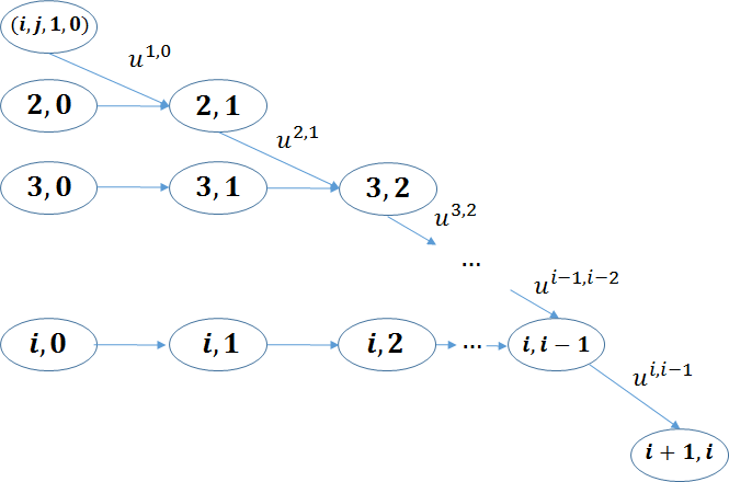
Figure 6.1. The states considered for the same $(i,j)$ pair, $0\leq i$,$0\leq j$ and their transition relations.

To describe the transition probabilities, assume the state of the selected node at step $k+1$ is $W_{k+1}=(i,j,c,l)$, for $k=0,\ldots,m-1$, there are three possibilities:

1. The selected node has defaulted, i.e $c\leq l$ or the node is invulnerable, i.e. $c>i$, then $S_{k+1}=S_{k},IT_{k+1}=IT_{k}$.

2. The selected node is vulnerable but has the “distance to default” more than one, i.e $c-l\geq 2$, then the node $w$ is selected with probability $\frac{(i-l)S_{k}^{i,j,c,l}}{m-k}$ and

   $$S_{k+1}^{i,j,c,l} = S_{k}^{i,j,c,l}-1,$$

   $$S_{k+1}^{i,j,c,l+1} = S_{k}^{i,j,c,l+1}+1,$$

   (6.0.2) $$IT_{k+1} = IT_{k},$$

   while other entries of $S_{k+1}$ are the same as $S_{k}$.

3. The selected node has the “distance to default” of one, i.e $c-l=1$, then the node is selected with probability $\frac{(i-c+1)S_{k}^{i,j,c,c-1}}{m-k}$ and by 2,

   $$S_{k+1}^{i,j,c,c-1} = S_{k}^{i,j,c,c-1}-1,$$

   $$S_{k+1}^{i,j,c+1,c} = S_{k}^{i,j,c+1,c}+g_{k+1}^{(n)}(S_{k},(i,j,c,c-1))$$

   $$= S_{k}^{i,j,c+1,c}+u^{i,j,c,c-1}(\frac{k}{n}),$$

   (6.0.3) $$IT_{k+1} = IT_{k}+u^{i,j,c,c-1}(\frac{k}{n}),$$

   while other entries of $S_{k+1}$ are the same as $S_{k}$.

Let $(\mathcal{F}_{k})_{k=0,\ldots,m}$ be the natural filtration of $S_{k}$, $\Delta S_{k}^{\alpha}=S_{k+1}^{\alpha}-S_{k}^{\alpha}$, $\alpha\in\Gamma$ and $\Delta IT_{k}=IT_{k+1}-IT_{k}$, it follows that

$$E\left[\Delta S{}_{k}^{i,j,c,0}|\mathcal{F}_{k}\right] = -\frac{iS_{k}^{i,j,c,0}}{m-k}\qquad\text{for $1\leq c\leq i$},$$

$$E\left[\Delta S_{k}^{i,j,c,l}|\mathcal{F}_{k}\right] = \frac{(i-l+1)S_{k}^{i,j,c,l-1}}{m-k}-\frac{(i-l)S_{k}^{i,j,c,l}}{m-k}$$

$$\text{ for }3\leq c\leq i,1\leq l\leq c-2,$$

$$E\left[\Delta S_{k}^{i,j,c,c-1}|\mathcal{F}_{k}\right] = \frac{(i-c+2)S_{k}^{i,j,c-1,c-2}}{m-k}u^{i,j,c-1,c-2}(\frac{k}{n})$$

$$+\frac{(i-c+2)S_{k}^{i,j,c,c-2}}{m-k}-\frac{(i-c+1)S_{k}^{i,j,c,c-1}}{m-k}$$

$$\text{ for }2\leq c\leq i,$$

$$E\left[\Delta S_{k}^{i,j,i+1,i}|\mathcal{F}_{k}\right] = \frac{S_{k}^{i,j,i,i-1}}{m-k}u^{i,j,i,i-1}(\frac{k}{n}),$$

(6.0.4) $$E\left[\Delta IT_{k}|\mathcal{F}_{k}\right] = \sum_{(i,j,c,c-1)\in\Phi}\frac{(i-c+1)S_{k}^{i,j,c,c-1}}{m-k}u^{i,j,c,c-1}(\frac{k}{n}).$$

7. Convergence of the default contagion process with interventions

Definition 7.1.

(ODEs of $s_{\tau}$) Given a set of piecewise constant function $u=(u^{\beta})_{\beta\in\Phi}$ on $[0,\lambda]$, i.e. $u\in\Pi$, define the system of ordinary differential equations (ODEs) of $s_{\tau}=(s_{\tau}^{\alpha})_{\alpha\in\Gamma}$ as

$$\frac{ds_{\tau}^{i,j,c,0}}{d\tau} = -\frac{is_{\tau}^{i,j,c,0}}{\lambda-\tau}\qquad\text{for $1\leq c\leq i$},$$

$$\frac{ds_{\tau}^{i,j,c,l}}{d\tau} = \frac{(i-l+1)s_{\tau}^{i,j,c,l-1}}{\lambda-\tau}-\frac{(i-l)s_{\tau}^{i,j,c,l}}{\lambda-\tau}$$

$$\text{ for }3\leq c\leq i,1\leq l\leq c-2,$$

$$\frac{ds_{\tau}^{i,j,c,c-1}}{d\tau} = \frac{(i-c+2)s_{\tau}^{i,j,c-1,c-2}}{\lambda-\tau}u^{i,j,c-1,c-2}(\tau)+\frac{(i-c+2)s_{\tau}^{i,j,c,c-2}}{\lambda-\tau}-\frac{(i-c+1)s_{\tau}^{i,j,c,c-1}}{\lambda-\tau}$$

$$\text{ for }2\leq c\leq i,$$

$$\frac{ds_{\tau}^{i,j,i+1,i}}{d\tau} = \frac{s_{\tau}^{i,j,i,i-1}}{\lambda-\tau}u^{i,j,i,i-1}(\tau).$$

The ODEs can be expressed in the form $\frac{ds_{\tau}}{d\tau}=h(\tau,s_{\tau};u_{\tau})$ where $h=(h^{\alpha})_{\alpha\in\Gamma}$.

For what is needed below we analyze the solutions of the ODEs in 7.1 for a subinterval of $[0,\lambda]$ where $u(\tau)$ is a constant vector function.

Proposition 7.1.

Let $s_{\tau}=(s_{\tau}^{\alpha})_{\alpha\in\Gamma}$ satisfy the system of ordinary differential equations in 7.1 with the initial conditions $s_{\tau_{1}}=s_{1}\coloneqq(s_{1}^{\alpha})_{\alpha\in\Gamma}$ in the interval on $[\tau_{1},\tau_{2})\subseteq[0,\lambda)$ and assume $u(\tau)$ is a constant vector function $u(\tau)=b\coloneqq(b^{\beta})_{\beta\in\Phi}$ where $b^{\beta}\in\{0,1\}$ on $[\tau_{1},\tau_{2})$, then the solution $s_{\tau}$ on $[\tau_{1},\tau_{2})$ is

$$s_{\tau}^{i,j,c,l} =(\frac{\lambda-\tau}{\lambda-\tau_{1}})^{i-l}\sum_{r=0}^{l}s_{1}^{i,j,c,r}\binom{i-r}{l-r}(1-\frac{\lambda-\tau}{\lambda-\tau_{1}})^{l-r}$$

(7.0.2) $$\text{ for }2\leq c\leq i,\;0\leq l\leq c-2,$$

$$s_{\tau}^{i,j,c,c-1} =(\frac{\lambda-\tau}{\lambda-\tau_{1}})^{i-c+1}\sum_{r=0}^{c-1}\sum_{q=r+1}^{c}\prod_{k=q}^{c-1}b^{i,j,k,k-1}s_{1}^{i,j,q,r}\binom{i-r}{c-1-r}(1-\frac{\lambda-\tau}{\lambda-\tau_{1}})^{c-1-r}$$

(7.0.3) $$\text{ for }1\leq c\leq i,$$

$$s_{\tau}^{i,j,i+1,i} =s_{1}^{i,j,i+1,i}+\sum_{r=0}^{i-1}\sum_{q=r+1}^{i}\prod_{k=q}^{i}b^{i,j,k,k-1}s_{1}^{i,j,q,r}(1-\frac{\lambda-\tau}{\lambda-\tau_{1}})^{i-r}$$

where $\prod_{k=c}^{c-1}b^{i,j,k,k-1}\coloneqq 1$. As a direct result, if we take the initial condition $s_{1}^{i,j,c,l}=p(i,j,c)\mathbbm{1}_{(l=0)}$ for $(i,j,c,l)\in\Gamma$ at $\tau_{1}=0$ , it follows that

$$s_{\tau}^{i,j,c,l} =p(i,j,c)\binom{i}{l}(1-\frac{\tau}{\lambda})^{i-l}(\frac{\tau}{\lambda})^{l}$$

(7.0.5) $$\text{ for }2\leq c\leq i,\;1\leq l\leq c-2.$$

We delegate the proof in 11.

In the following part our goal is to approximate $\frac{IT_{k}}{n}$ and $\frac{D_{k}}{n}$ as $n\rightarrow\infty$ given a function $u$. However, the number of variables depends on $n$, so we need to bound the terms associated with large in or out degree values. Fix $\epsilon>0$ and by 1 we have that

(7.0.6) $$\lambda=\sum_{i,j,c}ip(i,j,c)=\sum_{i,j,c}jp(i,j,c)<\infty,$$

then there exists an integer $M^{\epsilon}$ such that

(7.0.7) $$\sum_{i\geq M^{\epsilon}}\sum_{j,c}ip(i,j,c)+\sum_{j\geq M^{\epsilon}}\sum_{i,c}jp(i,j,c)<\epsilon,$$

so

$$\sum_{i\lor j\geq M^{\epsilon},c}jp(i,j,c)$$

$$= \sum_{i\geq M^{\epsilon}}\sum_{j<M^{\epsilon}}\sum_{c}jp(i,j,c)+\sum_{i\geq M^{\epsilon}}\sum_{j\geq M^{\epsilon}}\sum_{c}jp(i,j,c)+\sum_{i<M^{\epsilon}}\sum_{j\geq M^{\epsilon}}\sum_{c}jp(i,j,c)$$

$$\leq \sum_{i\geq M^{\epsilon}}\sum_{j<M^{\epsilon}}\sum_{c}ip(i,j,c)+\sum_{i\geq M^{\epsilon}}\sum_{j\geq M^{\epsilon}}\sum_{c}jp(i,j,c)+\sum_{i<M^{\epsilon}}\sum_{j\geq M^{\epsilon}}\sum_{c}jp(i,j,c)$$

$$< \epsilon.$$

We can prove similarly that there exists an integer $L^{\epsilon}$ such that $\sum_{i\lor j\geq L^{\epsilon},c}ip(i,j,c)<\epsilon$, but without loss of generality we write $M^{\epsilon}$ instead of $L^{\epsilon}$ in what follows. Moreover, by 1, as $n\rightarrow\infty$,

(7.0.9) $$\sum_{i,j,c}iP_{n}(i,j,c)=\sum_{i,j,c}jP_{n}(i,j,c)\rightarrow\lambda<\infty,$$

so for $n$ large enough, we can show that

$$\sum_{i\lor j\geq M^{\epsilon},c}jP_{n}(i,j,c) <\epsilon,$$

(7.0.10) $$\sum_{i\lor j\geq M^{\epsilon},c}iP_{n}(i,j,c) <\epsilon.$$

So we define the integer $M^{\epsilon}$ formally.

Definition 7.2.

For any $\epsilon>0$, we define $M^{\epsilon}$ as the integer such that

$$\sum_{i\lor j\geq M^{\epsilon},c}ip(i,j,c) <\epsilon,$$

$$\sum_{i\lor j\geq M^{\epsilon},c}jp(i,j,c) <\epsilon.$$

Accordingly, define

$$\Gamma^{\epsilon} \coloneqq\{(i,j,c,l):i\lor j<M^{\epsilon},0\leq l<c\leq i\text{ or }c=i+1,l=i\},$$

$$\Phi^{\epsilon} \coloneqq\{(i,j,c,c-1):i\lor j<M^{\epsilon},0\leq c\leq i\},$$

$$\hat{\lambda} \coloneqq\lambda-\epsilon,$$

where $a\lor b=\max\{a,b\}$.

Next we show that the scaled state variable $S_{k}$ and $IT_{k}$ converges in probability to the solution of the ODEs in 7.1 given the function $u$.

Proposition 7.2.

Consider a sequence of networks with initial conditions $(P_{n})_{n\geq 1}$ satisfying 1 and let $(G_{n})_{n\geq 1}$ be the sequence of control policies for the contagion process on the sequence of networks and $(G_{n})_{n\geq 1}$ satisfy 2 with the function $u=(u^{\beta})_{\beta\in\Phi^{\epsilon}}$, then

$$\sup_{0\leq k\leq n\hat{\lambda}}\frac{S_{k}^{\alpha}}{n}-s_{\frac{k}{n}}^{\alpha} = O(n^{-\frac{1}{4}}),$$

(7.0.11) $$\sup_{0\leq k\leq n\hat{\lambda}}\frac{\tilde{IT}_{k}}{n}-it_{\frac{k}{n}}^{\epsilon} = O(n^{-\frac{1}{4}}),$$

with probability $1-O(n^{\frac{1}{4}}\exp(-n^{\frac{1}{4}}))$ for $\alpha\in\Gamma^{\epsilon}$, where $s_{\tau}=(s_{\tau}^{\alpha})_{\alpha\in\Gamma^{\epsilon}}$ is the solution for the ODEs in 7.1 with the initial conditions $s_{0}^{i,j,c,l}=p(i,j,c)\mathbbm{1}_{(l=0)}$ and

$$\tilde{IT_{0}} =0,$$

$$\tilde{IT}_{k} =\sum_{l=1}^{k}\sum_{\beta\in\Phi^{\epsilon}}\mathbbm{1}_{(W_{\ell}=\beta)}u^{\beta}(\frac{\ell}{n}),$$

and

(7.0.12) $$\tilde{it}_{\tau} =\int_{0}^{\tau}\sum_{(i,j,c,c-1)\in\Phi^{\epsilon}}\frac{(i-c+1)s_{t}^{i,j,c,c-1}}{\lambda-t}u^{i,j,c,c-1}(t)dt.$$

From 7.2 we see that given $(P_{n})_{n\geq 1}$ and $(G_{n})_{n\geq 1}$ satisfying 1 and 2, respectively, the scaled stochastic process $\frac{S_{k}}{n}$ converges to the deterministic process $s_{\frac{k}{n}}$ for any $k$ in $[0,n\hat{\lambda}]$. This justifies the control policy we consider in 2 because given a control policy $G_{n}$ depending on the function $u$, we can predict with high probability the scaled stochastic contagion process at any time $k$. The proof of 7.2 is delegated to 11.

Next we discuss the convergence of the scaled number of defaults and the process end time.

Definition 7.3.

Define $D_{k}^{-}$ as the number of unrevealed out links from the default set at step $k$.

Recall that $D_{k}$ denotes the number of defaulted nodes at step $k$ which consist of two parts: the nodes that have defaulted initially $n\sum_{i,j}P_{n}(i,j,0)$ and those nodes that are vulnerable initially and default by step $k$, i.e. $n\sum_{i,j,1\leq c\leq i}P_{n}(i,j,c)-\sum_{(i,j,c,l)\in\Gamma}S_{k}^{i,j,c,l}$, thus

(7.0.13) $$D_{k} = n\sum_{i,j}P_{n}(i,j,0)+n\sum_{i,j,1\leq c\leq i}P_{n}(i,j,c)-\sum_{(i,j,c,l)\in\Gamma}S_{k}^{i,j,c,l}$$

$$= n\sum_{i,j,0\leq c\leq i}P_{n}(i,j,c)-\sum_{(i,j,c,l)\in\Gamma}S_{k}^{i,j,c,l}.$$

Similarly, among all defaulted nodes at step $k$ the nodes with out degree $j$ consist of two parts: the nodes that have defaulted initially $n\sum_{i}P_{n}(i,j,0)$ and those nodes that are vulnerable initially and default by step $k$, $n\sum_{i,1\leq c\leq i}P_{n}(i,j,c)-\sum_{i,0\leq l<c\leq i}S_{k}^{i,j,c,l}$, thus

(7.0.14) $$D_{k}^{-} = \sum_{j}j(n\sum_{i}P_{n}(i,j,0)+n\sum_{i,1\leq c\leq i}P_{n}(i,j,c)-\sum_{i,0\leq l<c\leq i}S_{k}^{i,j,c,l})-k$$

$$= n\sum_{i,j,0\leq c\leq i}jP_{n}(i,j,c)-\sum_{(i,j,c,l)\in\Gamma}jS_{k}^{i,j,c,l}-k.$$

Correspondingly we make the following definitions to approximate $\frac{D_{k}}{n}$ and $\frac{D_{k}^{-}}{n}$ as $n\rightarrow\infty$.

Definition 7.4.

Define

$$d_{\tau} = \sum_{i,j,0\leq c\leq i}p(i,j,c)-\sum_{(i,j,c,l)\in\Gamma}s_{\tau}^{i,j,c,l}$$

$$d_{\tau}^{-} = \sum_{i,j,0\leq c\leq i}jp(i,j,c)-\sum_{(i,j,c,l)\in\Gamma}js_{\tau}^{i,j,c,l}-\tau.$$

Proposition 7.3.

Based on 7.3 and 7.4, it follows that

$$\sup_{0\leq k\leq n\hat{\lambda}}\left|\frac{D_{k}^{-}}{n}-d_{\frac{k}{n}}^{-}\right| \leq o_{p}(1)+2\epsilon,$$

(7.0.16) $$\sup_{0\leq k\leq n\hat{\lambda}}\left|\frac{D_{k}}{n}-d_{\frac{k}{n}}\right| \leq o_{p}(1)+2\epsilon.$$

Proof.

For some $[\tau_{1},\tau_{2})\subseteq[0,\lambda)$ on which $u(\tau)$ is a constant vector function, from 7.1 we can show by summing all $s_{\tau}^{i,j,c,l}$, $(i,j,c,l)\in\Gamma$ with the same $(i,j)$ that

(7.0.17) $$0\leq\sum_{c,l}s_{\tau}^{i,j,c,l}\leq\sum_{c,l}s_{\tau_{1}}^{i,j,c,l},$$

so by induction we have

(7.0.18) $$\sum_{c,l}s_{\tau}^{i,j,c,l}\leq\sum_{1\leq c\leq i}p(i,j,c)$$

and thus it follows from (LABEL:eq:HighOrderTerms_p) that

$$0\leq \sum_{i\lor j\geq M^{\epsilon}}\sum_{0\leq c\leq i}jp(i,j,c)-\sum_{(i,j,c,l)\in\Gamma\backslash\Gamma^{\epsilon}}js_{\tau}^{i,j,c,l}$$

(7.0.19) $$\leq \sum_{i\lor j\geq M^{\epsilon}}\sum_{0\leq c\leq i}jp(i,j,c)<\epsilon.$$

Similarly because by the definition of $S_{k}^{i,j,c,l}$ for $1\leq k\leq m$, for fixed $(i,j)$ pair, $(i,j,c,l)\in\Gamma$,

(7.0.20) $$0\leq\sum_{c,l}\frac{S_{k}^{i,j,c,l}}{n}\leq\sum_{1\leq c\leq i}P_{n}(i,j,c),$$

thus it follows from (LABEL:HighOrderTerms_Pn) that

$$0\leq \sum_{i\lor j\geq M^{\epsilon}}\sum_{0\leq c\leq i}jP_{n}(i,j,c)-\sum_{(i,j,c,l)\in\Gamma\backslash\Gamma^{\epsilon}}j\frac{S_{k}^{i,j,c,l}}{n}$$

(7.0.21) $$\leq \sum_{i\lor j\geq M^{\epsilon}}\sum_{0\leq c\leq i}jP_{n}(i,j,c)<\epsilon.$$

For any $k$ where $0\leq k\leq\hat{\lambda}$, by 7.2 it follows that

$$\left|\frac{D_{k}^{-}}{n}-d_{\frac{k}{n}}^{-}\right| = |\sum_{i\lor j<M^{\epsilon},0\leq c\leq i}jP_{n}(i,j,c)-\sum_{(i,j,c,l)\in\Gamma^{\epsilon}}j\frac{S_{k}^{i,j,c,l}}{n}-$$

$$-(\sum_{i\lor j<M^{\epsilon},0\leq c\leq i}jp(i,j,c)-\sum_{(i,j,c,l)\in\Gamma^{\epsilon}}js_{\frac{k}{n}}^{i,j,c,l})|+2\epsilon$$

$$= \left|\sum_{i\lor j<M^{\epsilon},0\leq c\leq i}j\left(P_{n}(i,j,c)-p(i,j,c)\right)-\sum_{(i,j,c,l)\in\Gamma^{\epsilon}}j\left(\frac{S_{k}^{i,j,c,l}}{n}-s_{\frac{k}{n}}^{i,j,c,l}\right)\right|+2\epsilon$$

$$\leq \sum_{i\lor j<M^{\epsilon},0\leq c\leq i}j\left|P_{n}(i,j,c)-p(i,j,c)\right|+\sum_{(i,j,c,l)\in\Gamma^{\epsilon}}j\left|\frac{S_{k}^{i,j,c,l}}{n}-s_{\frac{k}{n}}^{i,j,c,l}\right|+2\epsilon$$

$$\leq M^{\epsilon}|\Gamma^{\epsilon}|\left(o(1)+o_{p}(1)\right)+2\epsilon=o_{p}(1)+2\epsilon,$$

and similarly,

$$\left|\frac{D_{k}}{n}-d_{\frac{k}{n}}\right| \leq \left|\sum_{i\lor j<M^{\epsilon},0\leq c\leq i}P_{n}(i,j,c)-\sum_{(i,j,c,l)\in\Gamma^{\epsilon}}\frac{S_{k}^{i,j,c,l}}{n}-(\sum_{i\lor j<M^{\epsilon},0\leq c\leq i}p(i,j,c)-\sum_{(i,j,c,l)\in\Gamma^{\epsilon}}s_{\frac{k}{n}}^{i,j,c,l})\right|$$

$$+2\epsilon$$

$$= \left|\sum_{i\lor j<M^{\epsilon},0\leq c\leq i}\left(P_{n}(i,j,c)-p(i,j,c)\right)-\sum_{(i,j,c,l)\in\Gamma^{\epsilon}}\left(\frac{S_{k}^{i,j,c,l}}{n}-s_{\frac{k}{n}}^{i,j,c,l}\right)\right|+2\epsilon$$

$$\leq \sum_{i\lor j<M^{\epsilon},0\leq c\leq i}\left|P_{n}(i,j,c)-p(i,j,c)\right|+\sum_{(i,j,c,l)\in\Gamma^{\epsilon}}\left|\frac{S_{k}^{i,j,c,l}}{n}-s_{\frac{k}{n}}^{i,j,c,l}\right|+2\epsilon$$

$$\leq |\Gamma^{\epsilon}|\left(o(1)+o_{p}(1)\right)+2\epsilon=o_{p}(1)+2\epsilon.$$

∎

To summarize the results we have so far, we have shown in 7.2 and (7.3) that the state variable $S_{k}$, the accumulative interventions $IT_{k}$, the number of defaults $D_{k}$ and the number of unrevealed out links from the default set $D_{k}^{-}$ after being scaled by $n$ all converge to a deterministic process which depends on the solution of the system of ODEs in 7.1. This convergence applies to any $k$ before $n\hat{\lambda}$. Recall that $IT_{n}\coloneqq IT_{T_{n}}$ and $D_{n}\coloneqq D_{T_{n}}$. By 7.3, $T_{n}=\min\{0\leq k\leq m:D_{k}^{-}=0\}$. Additionally define $\tau_{f}=\inf\{0\leq\tau\leq\lambda:d_{\tau}^{-}=0\}$. Next we show that when $\frac{T_{n}}{n}$ converges to $\tau_{f}$, then $\frac{IT_{n}}{n}$ and $\frac{D_{n}}{n}$ also converge in probability to the corresponding deterministic variables, $it_{\tau_{f}}$ and $d_{\tau_{f}}$, which in light of the boundedness of $\frac{IT_{n}}{n}$ and $\frac{D_{n}}{n}$ further implies convergence in expectations.

Proposition 7.4.

Consider a sequence of networks with initial conditions $(P_{n})_{n\geq 1}$ satisfying 1 and let $(G_{n})_{n\geq 1}$ be the sequence of control policies for the contagion processes on the sequence of networks and $(G_{n})_{n\geq 1}$ satisfy 2 with the function $u$. If $\tau_{f}=\lambda$, or $\tau_{f}<\lambda$ and $\frac{d}{d\tau}d_{\tau_{f}}^{-}<0$, it follows that as $n\rightarrow\infty$,

$$\frac{IT_{n}(G_{n},P_{n})}{n} \overset{p}{\rightarrow} it_{\tau_{f}}(u,p),$$

(7.0.24) $$\frac{D_{n}(G_{n},P_{n})}{n} \overset{p}{\rightarrow} d_{\tau_{f}}(u,p).$$

where

(7.0.25) $$it_{\tau_{f}} =\int_{0}^{\tau_{f}}\sum_{(i,j,c,c-1)\in\Phi}\frac{(i-c+1)s_{t}^{i,j,c,c-1}}{\lambda-t}u^{i,j,c,c-1}(t)dt.$$

Further it follows that as $n\rightarrow\infty$,

$$\mathbb{E}\frac{IT_{n}(G_{n},P_{n})}{n} \rightarrow it_{\tau_{f}}(u,p),$$

(7.0.26) $$\mathbb{E}\frac{D_{n}(G_{n},P_{n})}{n} \rightarrow d_{\tau_{f}}(u,p).$$

Proof.

By (7.0.10) for $n$ large enough and $1\leq k\leq m$, we have

$$\frac{1}{n}\sum_{\ell=1}^{k}\sum_{i\lor j\geq M^{\epsilon}}\sum_{1\leq c\leq i}\mathbbm{1}_{(W_{\ell}=(i,j,c,c-1))}u^{i,j,c,c-1}(\frac{\ell}{n})$$

$$\leq \frac{1}{n}\sum_{i\lor j\geq M^{\epsilon}}\sum_{1\leq c\leq i}iS_{k}^{i,j,c,c-1}$$

$$\leq \sum_{i\lor j\geq M^{\epsilon},c}iP_{n}(i,j,c)<\epsilon.$$

Similarly by (LABEL:eq:HighOrderTerms_p), for $\tau<\hat{\lambda}$,

$$\int_{0}^{\tau}\sum_{i\lor j\geq M^{\epsilon},1\leq c\leq i}\frac{(i-c+1)s_{t}^{i,j,c,c-1}}{\lambda-t}u^{i,j,c,c-1}(t)dt$$

$$\leq \int_{0}^{\tau}\sum_{i\lor j\geq M^{\epsilon},1\leq c\leq i}\frac{ip(i,j,c)}{\lambda-t}dt$$

$$\leq \epsilon\int_{0}^{\tau}\frac{1}{\lambda-t}dt$$

$$= \epsilon\ln\frac{\lambda}{\lambda-\tau}$$

$$\leq \epsilon\ln\frac{\lambda}{\epsilon}=O(\epsilon).$$

For any $k$ where $0\leq k\leq n\hat{\lambda}$, by 7.2 it follows that

$$\left|\frac{IT_{k}}{n}-it_{\frac{k}{n}}\right| \leq|\frac{\tilde{IT}_{k}}{n}+\frac{1}{n}\sum_{\ell=1}^{k}\sum_{i\lor j\geq M^{\epsilon}}\sum_{1\leq c\leq i}\mathbbm{1}_{(W_{\ell}=(i,j,c,c-1))}u^{i,j,c,c-1}(\frac{\ell}{n})$$

$$-(\tilde{it}_{\frac{k}{n}}+\int_{0}^{\tau}\sum_{i\lor j\geq M^{\epsilon},1\leq c\leq i}\frac{(i-c+1)s_{t}^{i,j,c,c-1}}{\lambda-t}u^{i,j,c,c-1}(t)dt)|$$

$$\leq\left|\frac{\tilde{IT}_{k}}{n}-\tilde{it}_{\frac{k}{n}}\right|+O(\epsilon)$$

$$\leq o_{p}(1)+O(\epsilon),$$

thus we have that

(7.0.27) $$\sup_{0\leq k\leq n\hat{\lambda}}\left|\frac{IT_{k}}{n}-it_{\frac{k}{n}}\right| =o_{p}(1)+O(\epsilon).$$

If $\tau_{f}=\lambda$, it implies that $d_{\tau}^{-}>0$ for $\tau\in(0,\hat{\lambda})$, then it follows from 7.3 that $\frac{T_{n}}{n}=\hat{\lambda}+O(\epsilon)+o_{p}(1)$. Then by the bounded change (11.2.3), $\frac{D_{T_{n}}}{n}=\frac{D_{\left\lfloor n\hat{\lambda}\right\rfloor}}{n}+O(\epsilon)+o_{p}(1)$ and from 7.3 again, $\frac{D_{\left\lfloor n\hat{\lambda}\right\rfloor}}{n}=d_{\hat{\lambda}}+O(\epsilon)+o_{p}(1)$. $\left\lfloor\cdot\right\rfloor$ denotes the floor function. Further by the continuity of $d_{\tau}$ on $[0,\lambda]$, $\frac{D_{T_{n}}}{n}=d_{\lambda}+O(\epsilon)+o_{p}(1)$. Similarly, by (7.0.27) and the continuity of $it_{\tau}$ on $[0,\lambda]$, we have that $\frac{IT_{T_{n}}}{n}=it_{\lambda}+O(\epsilon)+o_{p}(1)$.

If $\tau_{f}<\lambda$ and $\frac{d}{d\tau}d_{\tau_{f}}^{-}<0$, by 7.1, $s_{\tau}$ is continuous and thus by (LABEL:eq:EqOfdWithInt) $d_{\tau}^{-}$ is also continuous. So there exists some $\tau^{\prime}>0$ such that $d_{\tau}^{-}<0$ for $\tau\in(\tau_{f},\tau_{f}+\tau^{\prime})$ by the continuity of $d_{\tau}^{-}$. Since $\epsilon$ is arbitrary, let $\epsilon$ be small enough such that $\inf_{\tau\in(\tau_{f},\tau_{f}+\tau^{\prime})}d_{\tau}^{-}<-2\epsilon$ and $\hat{\tau}$ be the first time $d_{\tau}^{-}$ reaches the minimum. Because $d_{\hat{\tau}}^{-}<-2\epsilon$, then by 7.3 $\frac{D_{\left\lfloor n\hat{\tau}\right\rfloor}^{-}}{n}<0$ with high probability, so it holds that $\frac{T_{n}}{n}=\tau_{f}+O(\epsilon)+o_{p}(1)$. Again by the continuity of $d_{\tau}$ and $it_{\tau}$ on $[0,\lambda]$, 7.3 and (7.0.27), $\frac{D_{T_{n}}}{n}=d_{\tau_{f}}+O(\epsilon)+o_{p}(1)$ and $\frac{IT_{T_{n}}}{n}=it_{\tau_{f}}+O(\epsilon)+o_{p}(1)$.

Recall that $IT_{n}\coloneqq IT_{T_{n}}$ and $D_{n}\coloneqq D_{T_{n}}$. In both cases we conclude that (7.0.24) holds by tending $\epsilon\rightarrow 0$.

To prove (7.0.26), since $IT_{n}\leq m\leq(\lambda+0.1)n$ for large $n$ and $D_{n}\leq n$, $\frac{IT_{n}(G_{n},P_{n})}{n}$ and $\frac{D_{n}(G_{n},P_{n})}{n}$ are bounded and thus uniformly integrable. For a sequence of uniformly integrable random variables, convergence in probability implies convergence in expectation. Therefore (7.0.26) holds. ∎

Under the conditions in 7.4, the asymptotic control problem (ACP) becomes

(7.0.28) $$\min_{u\in\Pi}\>K\cdot it_{\tau_{f}}(u,p)+d_{\tau_{f}}(u,p).$$

In the following we write $u^{\beta}(\tau)=u_{\tau}^{\beta}$ and let $u_{\tau}=(u_{\tau}^{\beta})_{\beta\in\Phi}$ and $u=(u_{\tau})_{\tau\in[0,\lambda]}$.

Substituting the expressions of $it_{\tau_{f}}(u,p)$ and $d_{\tau_{f}}(u,p)$ in (7.0.25) and (LABEL:eq:EqOfdWithInt) respectively into (7.0.28) and putting together the system of ordinary differential equations of $s_{\tau}=(s_{\tau}^{\alpha})_{\alpha\in\Gamma}$, $\frac{d}{d\tau}s_{\tau}=h(\tau,s_{\tau};u_{\tau})$ in 7.1 as well as the condition that determines $\tau_{f}$, $d_{\tau_{f}}^{-}=0$, we attain the following deterministic optimal control problem.

(OCP) $$\min_{u,\tau_{f}} \;K\cdot it_{\tau_{f}}(u,p)+d_{\tau_{f}}(u,p)$$

st

$$\frac{d}{d\tau}s_{\tau}=h(\tau,s_{\tau};u_{\tau})$$

$$s_{0}^{i,j,c,l}=p(i,j,c)\mathbbm{1}_{(l=0)}$$

$$d_{\tau_{f}}^{-}=0$$

$$u_{\tau}^{\beta}\in\{0,1\}\;\forall\beta\in\Phi$$

$$\tau_{f}\in[0,\lambda),$$

where $\frac{d}{d\tau}s_{\tau}=h(\tau,s_{\tau};u_{\tau})$ is defined as in 7.1 with $u^{\beta}(\tau)=u_{\tau}^{\beta}$ and

$$it_{\tau_{f}}(u,p) =\int_{0}^{\tau_{f}}\sum_{i,j,1\leq c\leq i}\frac{(i-c+1)s_{\tau}^{i,j,c,c-1}}{\lambda-\tau}u_{\tau}^{i,j,c,c-1}d\tau,$$

$$d_{\tau_{f}}(u,p) =\sum_{i,j,0\leq c\leq i}p(i,j,c)-\sum_{(i,j,c,l)\in\Gamma}s_{\tau_{f}}^{i,j,c,l},$$

(7.0.29) $$d_{\tau_{f}}^{-} =\sum_{i,j,0\leq c\leq i}jp(i,j,c)-\sum_{(i,j,c,l)\in\Gamma}js_{\tau_{f}}^{i,j,c,l}-\tau_{f}.$$

Some difficulties arise because (OCP) is a infinite dimensional optimal control problem. We provide a two step algorithm to show that in light of 1, it suffices to solve a finite dimensional problem to approximate the objective function of the infinite dimensional problem. First we define the finite dimensional optimal control problem.

Definition 7.5.

For $\epsilon>0$, recall $M^{\epsilon}$ as in 7.2. Define the finite dimensional optimal control problem (FOCP) as (OCP) with the indexes $(i,j)$ restricted to $i\lor j<M^{\epsilon}$.

Remark 7.1.

The restriction of $(i,j)$ to $i\lor j<M^{\epsilon}$ indicates that we use only $p(i,j,c)$, $i\lor j<M^{\epsilon},$ $0\leq c\leq i$ in the calculation. It is equivalent to setting $p(i,j,c)=0$, $i\lor j\geq M^{\epsilon}$, $0\leq c\leq i$ while keeping $p(i,j,c)$, $i\lor j<M^{\epsilon}$, $0\leq c\leq i$ unchanged, which implies asymptotically nodes with $i\lor j\geq M^{\epsilon}$ are all invulnerable. By the solution of the ODE in 7.1, it implies that $s_{\tau}^{\beta}=0$, for $\beta\in\Gamma\backslash\Gamma^{\epsilon}.$ Note we use tilde sign with the variables to indicate the indexes $(i,j)$ are in the range $i\lor j<M^{\epsilon}$, for example, $\tilde{it}_{\tau_{f}}$, $\tilde{d}_{\tau_{f}}$ and $\tilde{d}_{\tau_{f}}^{-}$.

We have the following lemma regarding the objective functions of the infinite and finite dimensional optimal control problems.

Lemma 7.1.

Let $j(u,\tau_{f},p)\coloneqq K\,it_{\tau_{f}}(u,p)+d_{\tau_{f}}(u,p)$ be the objective function for the unrestricted (OCP) and $\tilde{j}(u,\tau_{f},p)\coloneqq K\,\tilde{it}{}_{\tau_{f}}(u,p)+\tilde{d}_{\tau_{f}}(u,p)$ for FOCP. Let $(u^{*},\tau_{f}^{*})$ be the optimal solution for the unrestricted (OCP) and $(\tilde{u},\tilde{\tau}_{f})$ be the optimal solution for FOCP, then for the same $p$ we have that

(7.0.30) $$\left|\tilde{j}(\tilde{u},\tilde{\tau}_{f},p)-j(u^{*},\tau_{f}^{*},p)\right|<(K+1)\epsilon.$$

Proof.

First we give an algorithm to construct a policy $u$ based on $\tilde{u}$. Let $(i,j,c,l)$ be the state of a node, so $i\lor j\geq M^{\epsilon}$ indicates that the node has either in or out degree greater than $M^{\epsilon}$ and $i\lor j<M^{\epsilon}$ indicates that the in and out degree is bounded by $M^{\epsilon}$.

Algorithm 1.

A two step algorithm.

1. Assume all nodes with $i\lor j\geq M^{\epsilon}$ are invulnerable for now. This is because as stated in 4.1, when constructing the configuration model sequentially, we have the freedom to reveal the out links only from the defaulted nodes with bounded degrees $i\lor j<M^{\epsilon}$ until all the out links from defaulted nodes with $i\lor j<M^{\epsilon}$ have been revealed. Let $\tilde{T}_{n}$ be the stopping time with $\tilde{D}_{\tilde{T}_{n}}$and $\tilde{IT}_{\tilde{T}_{n}}$ being the number of defaults and interventions by $\tilde{T}_{n}$, respectively. Accordingly we can solve FOCP for the optimal $(\tilde{u},\tilde{\tau}_{f})$ with the corresponding $\tilde{d}_{\tilde{\tau}_{f}}^{-}$. As in the proof of 7.4, assume that $\tilde{\tau}_{f}=\lambda$, or $\tilde{\tau}_{f}<\lambda$ and $\frac{d}{d\tau}\tilde{d}_{\tilde{\tau}_{f}}^{-}<0$, then $\frac{\tilde{T}_{n}}{n}\overset{p}{\rightarrow}\tilde{\tau}_{f}$.

2. But the nodes with $i\lor j\geq M^{\epsilon}$ may have defaulted by $\tilde{T}_{n}$. Next we look at these nodes, which consist of initially defaulted nodes with $i\lor j\geq M^{\epsilon}$ and those with $i\lor j\geq M^{\epsilon}$ that default because of the defaults of nodes with $i\lor j<M^{\epsilon}$ in the first step. Now we reveal their out links and we adopt a control policy to intervention at every step until the end of the contagion process $T_{n}$. Under this policy, there will be no additional defaults between $\tilde{T}_{n}$ and $T_{n}$. Recall $D_{T_{n}}$ and $IT_{T_{n}}$ are the number of defaults and interventions by $T_{n}$.

Through the above two steps, we construct a function $u$ as $u_{\tau}=\tilde{u}_{\tau}$, $\tau\leq\tilde{\tau}_{f}$ and $u_{\tau}^{\beta}=1$, $\tilde{\tau}_{f}<\tau$, $\beta\in\Phi$. Thus we have that

$$\frac{D_{T_{n}}}{n} =\frac{\tilde{D}_{\tilde{T}_{n}}}{n}+\frac{D_{T_{n}}-\tilde{D}_{\tilde{T}_{n}}}{n}$$

$$\leq\frac{\tilde{D}_{\tilde{T}_{n}}}{n}+\sum_{i\lor j\geq M^{\epsilon},0\leq c\leq i}P_{n}(i,j,c),$$

$$\frac{IT_{T_{n}}}{n} =\frac{\tilde{IT}{}_{\tilde{T}_{n}}}{n}+\frac{IT_{T_{n}}-\tilde{IT}{}_{\tilde{T}_{n}}}{n}$$

$$\leq\frac{\tilde{IT}{}_{\tilde{T}_{n}}}{n}+\sum_{i\lor j\geq M^{\epsilon},0\leq c\leq i}jP_{n}(i,j,c).$$

Note that the first inequality holds because the number of defaulted nodes with $i\lor j\geq M^{\epsilon}$ by $T_{n}$ is bounded above by the number of initially defaulted and initially vulnerable nodes with $i\lor j\geq M^{\epsilon}$. The second inequality holds because the number of interventions after $\tilde{T}_{n}$ is bounded above by the number of all out links from the nodes with $i\lor j\geq M^{\epsilon}$. Taking expectation on both sides and letting $n\rightarrow\infty$, from 7.4 and (7.0.10) it follows that

$$d_{\tau_{f}} \leq\tilde{d}_{\tilde{\tau}_{f}}+\epsilon,$$

$$it_{\tau_{f}} \leq\tilde{it}_{\tilde{\tau}_{f}}+\epsilon.$$

By the definition of $j$ and $\tilde{j}$,

(7.0.31) $$j(u,\tau_{f},p)\leq\tilde{j}(\tilde{u},\tilde{\tau}_{f},p)+(K+1)\epsilon.$$

Recall $(u^{*},\tau_{f}^{*})$ is the optimal solution for the unrestricted (OCP). Moreover, in the first step of 1 we treat all nodes with $i\lor j\geq M^{\epsilon}$ as invulnerable and $(\tilde{u},\tilde{\tau}_{f})$ is the optimal solution, so it provides the lower bound for the optimal objective function of the unrestricted (OCP), i.e.

(7.0.32) $$\tilde{j}(\tilde{u},\tilde{\tau}_{f},p)\leq j(u^{*},\tau_{f}^{*},p).$$

For the function $u$ we introduce through the two steps, we can calculate $\tau_{f}$ and the objective function value $j(u,\tau_{f},p)$. Then by the optimality of $(u^{*},\tau_{f}^{*})$, we have that

(7.0.33) $$j(u^{*},\tau_{f}^{*},p)\leq j(u,\tau_{f},p).$$

In sum, we have that

(7.0.34) $$\tilde{j}(\tilde{u},\tilde{\tau}_{f},p)\leq j(u^{*},\tau_{f}^{*},p)\leq j(u,\tau_{f},p)\leq\tilde{j}(\tilde{u},\tilde{\tau}_{f},p)+(K+1)\epsilon,$$

Thus the conclusion follows. ∎

By 7.1 we only need to solve the finite dimensional optimal control problem (FOCP) in 7.5. Because $\epsilon$ can be arbitrarily small, we can approximate the objective function of the infinite dimensional problem to any precision. Given $p$ for FOCP, the Pontryagin’s maximum principle provides the necessary conditions for the optimal control $\tilde{u}$ and end time $\tilde{\tau}_{f}$. We can obtain the optimal asymptotic number of interventions $\tilde{it}{}_{\tilde{\tau}_{f}}$ and fraction of final defaults $\tilde{d}{}_{\tilde{\tau}_{f}}$, which lead to the main results of our work. In the next section we focus on solving FOCP and suppress the tilde sign for the variables for notational convenience.

8. Necessary conditions for the optimal control problem

In the following we solve the finite dimensional optimal control problem (FOCP) in 7.5. Throughout this section we understand that the degrees are in the bounded range $i\lor j<M^{\epsilon}$ unless specified otherwise. We also suppress the tilde sign for notational convenience. Let $t=t(\tau)\coloneqq-\ln(\lambda-\tau)$, $t_{0}\coloneqq t(0)=-\ln\lambda$ and $t_{f}\coloneqq-\ln(\lambda-\tau_{f})$. Note $t(\tau)$ is a strictly increasing function of $\tau$ and so is the inverse function $\tau=\tau(t)$. We remark that we assume in the following that $\tau<\lambda$ which implies $t_{f}<\infty$, but later we can see that the solutions of $s_{\tau}$, $u_{\tau}$ and $w_{\tau}$ do allow $\tau=\lambda$. Then we can reformulate the optimal control problem (OCP) into an autonomous one, i.e. the differential equations of the system dynamics do not depend on time explicitly. Let $u_{t}=(u_{t}^{\beta})_{\beta\in\Phi^{\epsilon}}$ and without any confusion $u=(u_{t})_{t\geq t_{0}}$ (previously $u=(u_{\tau})_{\tau\in[0,\lambda]}$).

(AOCP) $$\min_{u,t_{f}} \;K\cdot it_{t_{f}}(u,p)+d_{t_{f}}(u,p)$$

st

$$\frac{d}{dt}s_{t}=h(s_{t};u_{t})$$

$$s_{t_{0}}^{i,j,c,l}=p(i,j,c)\mathbbm{1}_{(l=0)}$$

$$d_{t_{f}}^{-}=0$$

$$u_{t}^{\beta}\in\{0,1\}\;\forall\beta\in\Phi^{\epsilon}$$

$$t_{f}\in[0,\lambda),$$

where $\frac{d}{dt}s_{t}=h(s_{t};u_{t})$ denotes the system of differential equations

$$\frac{ds_{t}^{i,j,c,0}}{dt} =-is_{t}^{i,j,c,0}\text{ for }1\leq c\leq i,$$

$$\frac{ds_{t}^{i,j,c,l}}{dt} =(i-l+1)s_{t}^{i,j,c,l-1}-(i-l)s_{t}^{i,j,c,l}$$

$$\text{ for }3\leq c\leq i,\;1\leq l\leq c-2,$$

$$\frac{ds_{t}^{i,j,c,c-1}}{dt} =(i-c+2)s_{t}^{i,j,c-1,c-2}u_{t}^{i,j,c-1,c-2}+(i-c+2)s_{t}^{i,j,c,c-2}$$

$$-(i-c+1)s_{t}^{i,j,c,c-1}$$

$$\text{ for }2\leq c\leq i,$$

(8.0.2) $$\frac{ds_{t}^{i,j,i+1,i}}{dt} =s_{t}^{i,j,i,i-1}u_{t}^{i,j,i,i-1},$$

and

$$it_{t_{f}}(u,p) =\int_{t_{0}}^{t_{f}}\sum_{i,j,1\leq c\leq i}(i-c+1)s_{t}^{i,j,c,c-1}u_{t}^{i,j,c,c-1}dt,$$

$$d_{t_{f}}(u,p) =\sum_{i,j,0\leq c\leq i}p(i,j,c)-\sum_{(i,j,c,l)\in\Gamma^{\epsilon}}s_{t_{f}}^{i,j,c,l},$$

$$d_{t_{f}}^{-} =\sum_{i,j,0\leq c\leq i}jp(i,j,c)-\sum_{(i,j,c,l)\in\Gamma^{\epsilon}}js_{t_{f}}^{i,j,c,l}-\tau_{f}$$

(8.0.3) $$=\sum_{i,j,0\leq c\leq i}jp(i,j,c)-\sum_{(i,j,c,l)\in\Gamma^{\epsilon}}js_{t_{f}}^{i,j,c,l}-\lambda(1-e^{t_{0}-t_{f}}).$$

Note that (8.0.3) follows from $\frac{1}{\lambda}=e^{t_{0}}$ and thus $\tau_{f}=\lambda-e^{-t_{f}}=\lambda(1-\frac{1}{\lambda}e^{-t_{f}})=\lambda(1-e^{t_{0}-t_{f}})$.

To determine the necessary conditions for the optimal terminal time $t_{f}^{*}$ and optimal control $u_{t}^{*}$ in (AOCP), we need the extended Pontryagin maximum principle B.1 presented in the appendix. Then we put together the objective function (LABEL:eq:Obj_AOCP) and the necessary conditions to construct the optimization problem (OP) we will consider later.

Applying the extended Pontryagin maximum principle to the optimal control problem (AOCP) yields the following necessary conditions of optimality. Note in order to simplify notations, we suppress the apostrophe $"*"$ in the following. In other words, we use $s_{t},u_{t},w_{t},v,t_{f}$ instead of $s_{t}^{*},u_{t}^{*},w_{t}^{*},v^{*},t_{f}^{*}$ to denote the optimal values. First we present the correspondence of the notations in B.1 and our application.

Notation in B.1	Notation in our application
$t$	$t$
$t_{0}$	$t_{0}$
$t_{f}$	$t_{f}$
$(x_{t}^{i})_{i\in\{1,\ldots,n_{x}\}}$	$(s_{t}^{\alpha})_{\alpha\in\Gamma^{\epsilon}}$
$(u_{t}^{i})_{i\in\{1,\ldots,n_{u}\}}$	$(u_{t}^{\beta})_{\beta\in\Phi^{\epsilon}}$
$U$	$\{0,1\}$
$\mathring{\lambda}$	$\mathring{w}$
$(\lambda_{t}^{i})_{i\in\{1,\ldots,n_{x}\}}$	$(w_{t}^{\alpha})_{\alpha\in\Gamma^{\epsilon}}$
$\ell(t,x_{t},u_{t})$	$K\sum_{i,j,1\leq c\leq i}(i-c+1)s_{t}^{i,j,c,c-1}u_{t}^{i,j,c,c-1}$
$\phi(t_{f},x_{t_{f}})$	$d_{t_{f}}$
$\psi_{k}(t_{f},x_{t_{f}})=0,\quad k=1,\ldots,n_{\psi}$	$d_{t_{f}}^{-}=0$

Table 1. Correspondence of the notations in B.1 and 8.1.

Proposition 8.1.

(Necessary conditions of optimality) Let $(s_{t},u_{t})_{t\in[t_{0},t_{f}]}$ be the optimal state and control trajectory of (AOCP) where $t_{f}$ is the optimal terminal time. Define the Hamiltonian function

$$\mathcal{H}(s_{t},u_{t},w_{t}) = \sum_{i,j,1\leq c\leq i}w_{t}^{i,j,c,0}(-is_{t}^{i,j,c,0})$$

$$+\sum_{i,j,2\leq c\leq i,1\leq l\leq c-1}w_{t}^{i,j,c,l}\left[(i-l+1)s_{t}^{i,j,c,l-1}-(i-l)s_{t}^{i,j,c,l}\right]$$

$$+\sum_{i,j,2\leq c\leq i+1}(K+w_{t}^{i,j,c,c-1})(i-c+2)s_{t}^{i,j,c-1,c-2}u_{t}^{i,j,c-1,c-2},$$

then there exist a piecewise continuously differentiable vector function $w_{t}=(w_{t}^{\alpha})_{\alpha\in\Gamma^{\epsilon}}\in\hat{C}^{1}[t_{0},\infty)^{\left|\Gamma^{\epsilon}\right|}$ and a scalar $v\in\mathbb{R}$ such that the following conditions hold:

1. The optimal control $u_{t}$ satisfies that $\forall t\in[t_{0},t_{f}]$, $1\leq c\leq i$,

   (8.0.5)

   if $s_{t}^{i,j,c,c-1}>0$,

   $$u_{t}^{i,j,c,c-1} =\begin{cases}0&\text{ if }w_{t}^{i,j,c+1,c}>-K\\ 1&\text{ if }w_{t}^{i,j,c+1,c}<-K\\ 0\text{ or }1&\text{ if }w_{t}^{i,j,c+1,c}=-K,\end{cases}$$

   if $s_{t}^{i,j,c,c-1}=0$,

   $$u_{t}^{i,j,c,c-1} =0\text{ or }1.$$

2. For $2\leq c\leq i$, $0\leq l\leq c-2$,

   (8.0.6) $$\frac{d}{dt}w_{t}^{i,j,c,l}=(i-l)(w_{t}^{i,j,c,l}-w_{t}^{i,j,c,l+1}),$$

   and for $1\leq c\leq i$,

   (8.0.7) $$\frac{d}{dt}w_{t}^{i,j,c,c-1}=(i-c+1)(w_{t}^{i,j,c,c-1}-(K+w_{t}^{i,j,c+1,c})u_{t}^{i,j,c,c-1}),$$

   and

   (8.0.8) $$\frac{d}{dt}w_{t}^{i,j,i+1,i}=0.$$

   We denote the set of ordinary differential equations for $w_{t}$ as $\frac{d}{dt}w_{t}=h^{\prime}(w_{t};u_{t})$.

3. $\mathcal{H}(s_{t},u_{t},w_{t})$ is a constant for $t\in[t_{0},t_{f}]$.

4. Transversal conditions

   (8.0.9) $$w_{t_{f}}^{i,j,c,l} =vj-1\qquad\forall(i,j,c,l)\in\Gamma^{\epsilon},$$

   (8.0.10) $$\mathcal{H}(s_{t_{f}},u_{t_{f}},w_{t_{f}}) =-ve^{-t_{f}},$$

   $$d_{t_{f}}^{-} =\sum_{i,j,0\leq c\leq i}jp(i,j,c)-\sum_{(i,j,c,l)\in\Gamma^{\epsilon}}js_{t_{f}}^{i,j,c,l}-\lambda(1-e^{t_{0}-t_{f}})$$

   (8.0.11) $$=0.$$

Proof.

Let $(\mathring{w},w_{t})$ be the adjoint variables then $\mathring{w}=1$, since otherwise the necessary conditions of optimality becomes independent of the cost functional in (AOCP). The Hamiltonian function (LABEL:eq:Ham_NC) is a direct result of (B.0.6). Note that $n_{\psi}=1$ and

(8.0.12) $$\psi(t,s)=\sum_{i,j,0\leq c\leq i}jp(i,j,c)-\sum_{(i,j,c,l)\in\Gamma^{\epsilon}}js^{i,j,c,l}-\lambda(1-e^{t_{0}-t}).$$

Taking partial derivative yields $\frac{\partial}{\partial s}\psi(t_{f},s_{t_{f}})=(j,j,\ldots,j)$ which has rank $1$.

Since the Hamiltonian function is affine in the control variable $u_{t}$, by condition (1) of B.1, we attain that, for $1\leq c\leq i$,

(8.0.13) $$u_{t}^{i,j,c,c-1}=\begin{cases}0&\text{ if }(K+w_{t}^{i,j,c+1,c})s_{t}^{i,j,c,c-1}>0\\ 1&\text{ if }(K+w_{t}^{i,j,c+1,c})s_{t}^{i,j,c,c-1}<0\\ 0\text{ or }1&\text{if }(K+w_{t}^{i,j,c+1,c})s_{t}^{i,j,c,c-1}=0.\end{cases}$$

By distinguishing the two cases $s_{t}^{i,j,c,c-1}>0$ and $s_{t}^{i,j,c,c-1}=0$, we have the equivalent form in (8.0.5).

Taking partial derivative of $\mathcal{H}$ with regard to $s$ yields the differential equations of $w_{t}$ in condition (2). Note that $\mathcal{H}$ is autonomous, then according to condition (3) of B.1, $\mathcal{H}(s_{t},u_{t},w_{t})$ is a constant for $t\in[t_{0},t_{f}]$, which is condition (3).

Then define

$$\mbox{$\Psi$}(t,s) \coloneqq \sum_{i,j,0\leq c\leq i}p(i,j,c)-$$

$$\sum_{(i,j,c,l)\in\Gamma^{\epsilon}}s^{i,j,c,l}+v(\sum_{i,j,0\leq c\leq i}jp(i,j,c)-\sum_{(i,j,c,l)\in\Gamma^{\epsilon}}js_{t_{f}}^{i,j,c,l}-\lambda(1-e^{t_{0}-t_{f}}))$$

and taking partial derivatives with respect to $s$ and $t$ respectively by condition (4) of B.1 together with the terminal condition (8.0.3) leads to condition (4). ∎

Remark 8.1.

(Singular control policy) Observe that if the coefficient of $u_{t}^{i,j,c,c-1}$ in the Hamiltonian function $\mathcal{H}(s_{t},u_{t},w_{t})$ (LABEL:eq:Ham_NC), i.e. $(i-c+1)(K+w_{t}^{i,j,c+1,c})s_{t}^{i,j,c,c-1}$ vanishes, $u_{t}^{i,j,c,c-1}=0$ or $1$ both satisfy (1) of B.1, i.e. minimizing $\mathcal{H}(s_{t},u_{t},w_{t})$. In other words, the Pontryagin maximum principle in B.1 cannot determine the optimal control $u_{t}^{i,j,c,c-1}$ in this case. Moreover, since $i-c+1>0$, so if $(K+w_{t}^{i,j,c+1,c})s_{t}^{i,j,c,c-1}=0$ can be sustained over some interval $(\theta_{1},\theta_{2})\subset[t_{0},t_{f}]$, then $u_{t}^{i,j,c,c-1}$ can be $0$ or $1$ at any time on $(\theta_{1},\theta_{2})$ and switch arbitrarily often between $0$ and $1$. In the terminology of optimal control theory, the control $u_{t}$ is “singular” on $(\theta_{1},\theta_{2})$ and the corresponding portion of the state trajectory $s_{t}$ on $(\theta_{1},\theta_{2})$ is called a singular arc. Further note that $(K+w_{t}^{i,j,c+1,c})s_{t}^{i,j,c,c-1}=0$, $t\in(\theta_{1},\theta_{2})$ implies two cases: $s_{t}^{i,j,c,c-1}=0$ or $s_{t}^{i,j,c,c-1}>0$, $w_{t}^{i,j,c+1,c}=-K$, $t\in(\theta_{1},\theta_{2})$. We can show that in the first case any feasible control policy $u_{t}^{i,j,c,c-1}$ will not affect other entries of $s_{t}$ and the second case only occurs when $c=i$ and $(\theta_{1},\theta_{2})=(t_{0},t_{f})$.

Now the differential equations for $s_{t}$ in (AOCP) and $w_{t}$ in condition (2) of 8.1 constitute a two-point boundary value problem (TPBVP) because for $s_{t}$ the boundary values are given at $t=t_{0}$ while for $w_{t}$ at $t=t_{f}$ as follows

(TPBVP) $$\frac{d}{dt}s_{t} =h(s_{t};u_{t})$$

$$s_{t_{0}}^{i,j,c,l} =p(i,j,c)\mathbbm{1}_{(l=0)}\qquad\forall(i,j,c,l)\in\Gamma^{\epsilon}$$

$$\frac{d}{dt}w_{t} =h^{\prime}(w_{t};u_{t})$$

$$w_{t_{f}}^{i,j,c,l} =vj-1\qquad\forall(i,j,c,l)\in\Gamma^{\epsilon}$$

By solving the differential equations we are able to find the optimal control policy $(u_{t})_{t\in[t_{0},t_{f}]}$ stated in 10.2 and the optimal state trajectory $(s_{t})_{t\in[t_{0},t_{f}]}$ which leads to the conclusions of 10.3 about the optimal asymptotic fraction of final defaulted nodes.

9. Solutions of the necessary conditions

Throughout this section we understand that the degrees are in the bounded range $i\lor j<M^{\epsilon}$ unless specified otherwise. The main difficulty of solving the TPBVP arises from the fact that $w_{t}$ and $s_{t}$ depend on $u_{t}$ which depends on $w_{t}$ and $s_{t}$ recursively according to (1) of 8.1. To disentangle the recursive dependence, the idea is to analyze the properties of $s_{t}$ based on which we are able to either derive the properties of $w_{t}$ or provide explicit solutions of $w_{t}$ under different cases. By (1) of 8.1 we attain the optimal control policy $u_{t}$ which allows us to solve for $s_{t}$. At this point $(s_{t},u_{t},w_{t})$ are all expressed in terms of the variables $(v,t_{f},t_{s})$. Since the optimal $(s_{t},u_{t},w_{t})$ satisfies the two equations in the necessary conditions of 8.1, i.e. the Hamiltonian function (8.0.10) at $t=t_{f}$ and the terminal condition (8.0.11), while minimizing the objective function (LABEL:eq:Obj_AOCP), we have the following optimization problem for $(v,t_{f},t_{s})$.

(9.0.1) $$\min_{v,t_{f},t_{s}} K\cdot it_{t_{f}}(u,p)+d_{t_{f}}(u,p)$$

(9.0.3) st $$\mathcal{H}(s_{t_{f}},u_{t_{f}},w_{t_{f}})=-ve^{-t_{f}}$$

(9.0.4) $$d_{t_{f}}^{-}=0$$

$$t_{0}\leq t_{s}\leq t_{f}$$

$$v\in\mathbb{R},$$

where $s_{t}$, $u_{t}$ and $w_{t}$ are functions of $(v,t_{f},t_{s})$ and

$$it_{t_{f}}(u,p) =\int_{t_{0}}^{t_{f}}\sum_{i,j,1\leq c\leq i}(i-c+1)s_{t}^{i,j,c,c-1}u_{t}^{i,j,c,c-1}dt,$$

$$d_{t_{f}}(u,p) =\sum_{i,j,0\leq c\leq i}p(i,j,c)-\sum_{(i,j,c,l)\in\Gamma^{\epsilon}}s_{t_{f}}^{i,j,c,l},$$

(9.0.5) $$d_{t_{f}}^{-} =\sum_{i,j,0\leq c\leq i}jp(i,j,c)-\sum_{(i,j,c,l)\in\Gamma^{\epsilon}}js_{t_{f}}^{i,j,c,l}-\lambda(1-e^{t_{0}-t_{f}}).$$

After substituting $(s_{t},u_{t},w_{t})$ expressed in terms of $(v,t_{f},t_{s})$ into the optimization problem (9.0.1), we are able to solve the optimal $(v,t_{f},t_{s})$ based on which we can calculate the optimal $(s_{t},u_{t},w_{t})$. Further we change the variables from $(v,t_{f},t_{s})$ to $(v,y,z)$ to further simplify, thus we attain the optimization problem (OP) later.

It turns out that we only need $w_{t_{f}}$ as well as $u_{t}$ and $s_{t}$ in (9.0.1). From (TPBVP) we know that $w_{t_{f}}^{\beta}=vj-1$ for $\beta\in\Gamma^{\epsilon}$. For $u_{t}$ and $s_{t}$, we give out their solutions in the following directly due to the limited space of the paper.

Lemma 9.1.

The optimal control policy $u_{t}$ in terms of the variables $(v,t_{f},t_{s})$ is given as below.

For $1\leq c\leq i$ except $c=i$ when $vj-1=-K$, $\forall t\in[t_{0},t_{f}]$,

(9.0.6) $$u_{t}^{i,j,c,c-1}=\mathbbm{1}_{(t\geq t^{i,j,c})},$$

where

(9.0.7) $$t^{i,j,c}=\begin{cases}t_{f}&\text{ if }vj-1\geq-K\\ t_{f}+\ln\left(1+\frac{K+vj-1}{(i-c)K}\right)&\text{ if }vj-1<-K\text{ and }1\leq c<i+\frac{K+vj-1}{K(1-e^{t_{0}-t_{f}})}\\ t_{0}&\text{otherwise},\end{cases}$$

If $vj-1=-K$, $\forall t\in[t_{0},t_{f}]$,

(9.0.8) $$u_{t}^{i,j,i,i-1}=\mathbbm{1}_{(t\geq t_{s})}\text{ for some }t_{s}\in[t_{0},t_{f}].$$

The following is the solution for $s_{t}$.

Lemma 9.2.

Letting $p(i,j,i+1)=0$, under the optimal control policy in 9.1, we have the following solutions of $s_{t}$ for the two-point boundary value problem (TPBVP).

1. For $2\leq c\leq i$, $0\leq l\leq c-2$ and $c=1$, $l=0$,

   (9.0.9) $$s_{t}^{i,j,c,l}=p(i,j,c)\binom{i}{l}\left(e^{t_{0}-t}\right)^{i-l}(1-e^{t_{0}-t})^{l}.$$

2. If $vj-1<-K$, consider $t\in[t^{i,j,h},t^{i,j,h-1})$, for some $1\leq h\leq i$ where

   (9.0.10) $$t^{i,j,h}=\begin{cases}t_{f}&\text{if }h=0\\ t_{f}+\ln(1+\frac{K+vj-1}{(i-h)K})&\text{if }1\leq h<i+\frac{K+vj-1}{K(1-e^{t_{0}-t_{f}})}\\ t_{0}&\text{otherwise}.\end{cases}$$

   If $1\leq c<h$,

   (9.0.11) $$s_{t}^{i,j,c,c-1} =p(i,j,c)\binom{i}{c-1}\left(e^{t_{0}-t}\right)^{i-c+1}(1-e^{t_{0}-t})^{c-1}.$$

   If $h\leq c\leq i+1$,

   $$s_{t}^{i,j,c,c-1} =\binom{i}{c-1}\left(e^{t_{0}-t}\right)^{i-c+1}\sum_{m=h}^{c}p(i,j,m)$$

   $$\sum_{n=0}^{m-1}\binom{c-1}{n}\left(1-e^{t_{0}-t^{i,j,m}}\right)^{n}(e^{t_{0}-t^{i,j,m}}-e^{t_{0}-t})^{c-1-n}.$$

3. If $vj-1>-K$, for $1\leq c\leq i+1,$ $t\in[t_{0},t_{f}]$,

   (9.0.13) $$s_{t}^{i,j,c,c-1}=p(i,j,c)\binom{i}{c-1}\left(e^{t_{0}-t}\right)^{i-c+1}(1-e^{t_{0}-t})^{c-1}.$$

4. If $vj-1=-K$, for $1\leq c\leq i$, $t\in[t_{0},t_{f}]$,

   (9.0.14) $$s_{t}^{i,j,c,c-1}=p(i,j,c)\binom{i}{c-1}\left(e^{t_{0}-t}\right)^{i-c+1}(1-e^{t_{0}-t})^{c-1},$$

   and

   (9.0.15) $$s_{t}^{i,j,i+1,i}=p(i,j,i)\mathbbm{1}_{\{t_{s}\leq t)}[(1-e^{t_{0}-t})^{i}-(1-e^{t_{0}-t_{s}})^{i}],$$

   where $t_{s}\in[t_{0},t_{f}]$.

The solutions of $w_{t}$ and $s_{t}$ can be verified by substituting into (TPBVP). Since (8.0.11) and (8.0.10) require the state variable value particularly at $t=t_{f}$, we can apply 9.2 at $t=t_{f}$ to attain $s_{t_{f}}$. Next we substitute $s_{t}$, $u_{t}$ and $w_{t_{f}}$ into the optimization program (9.0.1) leading to the following results.

Proposition 9.1.

Based on the solutions of optimal $s_{t}$ in 9.2 (particularly $s_{t_{f}}$), $u_{t}$ in 9.1 and $w_{t_{f}}^{\beta}=vj-1$, $\forall\beta\in\Gamma^{\epsilon}$, letting

(9.0.16) $$t^{i,j,c}=\begin{cases}t_{f}&\text{if }K+vj-1\geq 0\text{ or }c=0\\ t_{f}+\ln(1+\frac{K+vj-1}{(i-c)K})&\text{if }K+vj-1<0\text{ and }1\leq c<i+\frac{K+vj-1}{K(1-e^{t_{0}-t_{f}})},\\ t_{0}&\text{otherwise},\end{cases}$$

the Hamiltonian equation (9.0.3) at $t=t_{f}$ is equivalent to

$$\sum_{j}\max\{-K,vj-1\}\sum_{i}i\sum_{c=1}^{i}p(i,j,c)\sum_{m=c}^{i}\binom{i-1}{m-1}\left(e^{t_{0}-t_{f}}\right)^{i-m+1}$$

$$\sum_{n=0}^{c-1}\binom{m-1}{n}\left(1-e^{t_{0}-t^{i,j,c}}\right)^{n}(e^{t_{0}-t^{i,j,c}}-e^{t_{0}-t_{f}})^{m-1-n}$$

$$= v\lambda e^{t_{0}-t_{f}}.$$

The terminal condition (9.0.4) is equivalent to

$$\sum_{i}\sum_{j}j\{\sum_{c=0}^{i}p(i,j,c)\sum_{n=c}^{i}\binom{i}{n}(1-e^{t_{0}-t^{i,j,c}})^{n}(e^{t_{0}-t^{i,j,c}})^{i-n}$$

$$-\mathbbm{1}_{(vj-1=-K)}p(i,j,i)[(1-e^{t_{0}-t_{f}})^{i}-(1-e^{t_{0}-t_{s}})^{i}]\}$$

$$= \lambda(1-e^{t_{0}-t_{f}}).$$

And the objective function (LABEL:eq:Obj_forOP)

$$K\cdot it_{t_{f}}(u,p)+d_{t_{f}}(u,p)$$

$$= K\sum_{i}\sum_{j}\{\sum_{c=1}^{i}p(i,j,c)$$

$$\sum_{m=c}^{i}\sum_{n=0}^{c-1}(m-c+1)\binom{i}{m}\binom{m}{n}(e^{t_{0}-t_{f}})^{i-m}\left(1-e^{t_{0}-t^{i,j,c}}\right)^{n}(e^{t_{0}-t^{i,j,c}}-e^{t_{0}-t_{f}})^{m-n}$$

$$+\mathbbm{1}_{(vj-1=-K)}p(i,j,i)[(1-e^{t_{0}-t_{f}})^{i}-(1-e^{t_{0}-t_{s}})^{i}]\}$$

$$+\sum_{j}\sum_{i}\{\sum_{c=0}^{i}p(i,j,c)\sum_{n=c}^{i}\binom{i}{n}(1-e^{t_{0}-t^{i,j,c}})^{n}(e^{t_{0}-t^{i,j,c}})^{i-n}$$

$$-\mathbbm{1}_{(vj-1=-K)}p(i,j,i)[(1-e^{t_{0}-t_{f}})^{i}-(1-e^{t_{0}-t_{s}})^{i}]\}.$$

We further simplify the expressions in 9.1. Define

$$y =1-e^{t_{0}-t_{f}},$$

$$z =1-e^{t_{0}-t_{s}},$$

$$x^{i,j,c,c-1} =1-e^{t_{0}-t^{i,j,c}}$$

$$=\begin{cases}y&\text{if }K+vj-1\geq 0\text{ or }c=0\\ 1-(1-y)\frac{(i-c)K}{(i-c+1)K+vj-1}&\text{if }K+vj-1<0\text{ and }1\leq c<i+\frac{K+vj-1}{Ky}\\ 0&\text{otherwise},\end{cases}$$

then because $t_{0}\leq t_{s}\leq t_{f}$ and the function $1-e^{t_{0}-t}$ is increasing in $t$, $0\leq z\leq y\leq 1$. As a result, we can substitute the new variables $(y,v,z)$ into the objective function (LABEL:eq:Obj_forOP), the Hamiltonian equation (9.0.3) and the terminal condition (9.0.4). Moreover, we add the definition of $x^{i,j,c,c-1}$ and $0\leq z\leq y\leq 1$ and as a result, we obtain a new optimization problem defined as (OP) in 10. After solving (OP) for $(y^{*},v^{*},z^{*})$, we are able to calculate $u_{t}^{*}$ and $s_{t}^{*}$ (or $u_{\tau}^{*}$ and $s_{\tau}^{*}$ after changing the time index) in order to present 10.2 and 10.3.

10. Main results

10.1. Contagion process with no interventions

We first present the theorem when no interventions are provided in the contagion process. For $\epsilon>0$, recall $M^{\epsilon}$ is defined as in 7.2 and note that all indexes $(i,j)$ are in the range $i\lor j<M^{\epsilon}$ in what follows.

Definition 10.1.

($I$ function) Define a function $I:\ [0,1]\rightarrow[0,1]$ as

(10.1.1) $$I(y)\coloneqq\frac{1}{\lambda}\sum_{i\lor j<M^{\epsilon}}j\sum_{c=0}^{i}p(i,j,c)\mathbb{P}(\text{Bin}(i,y)\geq c)$$

where $\text{Bin}(i,y)$ denotes a binomial random variable with $i$ trials and the probability of occurrence $y$, so $\mathbb{P}(\text{Bin}(i,y)\geq c)=\sum_{m=c}^{i}\binom{i}{m}y^{m}(1-y)^{i-m}$. $I(y)$ is constructed to represent the asymptotic scaled total out degree from the default set at scaled time $y$ and attains its form (10.1.1) from the solution of a set of differential equations. It can be interpreted as the expected number of defaults if an end node of a randomly selected directed link defaults with probability $y$.

Since $I(0)=\frac{1}{\lambda}\sum_{i\lor j<M^{\epsilon}}jp(i,j,0)\geq 0$, and from the definition of $\lambda$,

(10.1.2) $$I(1)=\frac{1}{\lambda}\sum_{i\lor j<M^{\epsilon}}j\sum_{c=0}^{i}p(i,j,c)\leq 1,$$

and $I(y)$ is continuous and increasing, it has at least one fixed point in $[0,1]$. Further define

(10.1.3) $$J(y)\coloneqq\sum_{i\lor j<M^{\epsilon}}\sum_{c=0}^{i}p(i,j,c)\mathbb{P}(\text{Bin}(i,y)\geq c).$$

Theorem 10.1.

(Extends from theorem 3.8 of Amini et al. (2013)) Consider a sequence of networks with initial conditions $(P_{n})_{n\geq 1}$ satisfying 1 where $p=(p(i,j,c))_{i,j,0\leq c\leq i}$ such that $p(i,j,c)=0$ for $i\lor j\geq M^{\epsilon},0\leq c\leq i$ and no interventions are implemented, let $y^{*}\in[0,1]$ be the smallest fixed point of $I$.

1. If $y^{*}=1$, then asymptotically almost all nodes default during the contagion process, i.e.

   (10.1.4) $$\frac{D_{n}}{n}\overset{p}{\to}1.$$

2. If $y^{*}<1$ and it is a stable fixed point, i.e. $I^{\prime}(y^{*})<1$, then asymptotically the fraction of final defaulted nodes

   (10.1.5) $$\frac{D_{n}}{n}\overset{p}{\to}J(y^{*}).$$

   Particularly, if $I(0)=0$ and $I^{\prime}(0)<1$, then

   (10.1.6) $$\frac{D_{n}}{n}\overset{p}{\to}\sum_{i\lor j<M^{\epsilon}}p(i,j,0).$$

Remark 10.1.

Theorem 10.1 states that the stopping time of the default contagion process is fully governed by the smallest fixed point of the function $I(y)$ and the asymptotic fraction of defaulted nodes at the end of the process can be 1, 0 or a fractional number, representing almost all nodes default, almost no nodes default or a partial number of nodes default, respectively.

10.2. Contagion process with interventions

We present the theorems for the contagion process with interventions as the result of solving the finite dimensional optimal control problem (FOCP) in 7.5. For $\epsilon>0$, recall $M^{\epsilon}$ is defined as in 7.2. By 7.1, the optimal objective function value of FOCP is within $(K+1)\epsilon$ distance to the optimal objective function value of the unrestricted (OCP). Note that all indexes $(i,j)$ are in the range $i\lor j<M^{\epsilon}$ in what follows. From 7.1, for a given vector $p=(p(i,j,c))_{0\leq i,0\leq j,0\leq c\leq i}$, the restriction of $(i,j)$ to $i\lor j<M^{\epsilon}$ indicates that we use only $p(i,j,c)$, $i\lor j<M^{\epsilon},$ $0\leq c\leq i$ in the calculation. It is equivalent to setting $p(i,j,c)=0$, $i\lor j\geq M^{\epsilon}$, $0\leq c\leq i$ while keeping $p(i,j,c)$, $i\lor j<M^{\epsilon}$, $0\leq c\leq i$ unchanged, which implies asymptotically nodes with $i\lor j\geq M^{\epsilon}$ are all invulnerable.

First we define the optimization problem (OP) based on which we present 10.2 and 10.3.

Definition 10.2.

($\tilde{I}$ and $\tilde{J}$ function) Let $x=(x^{\beta})_{\beta\in\Phi^{\epsilon}}$ where $x^{\beta}=x^{\beta}(y,v)$ and $p=(p(i,j,c))_{i,j,0\leq c\leq i}$. We define the functions $\tilde{I}(y,v,z)$ and $\tilde{J}(y,v,z)$ as

$$\tilde{I}(y,v,z) =\frac{1}{\lambda}\sum_{i\lor j<M^{\epsilon}}j$$

(10.2.1) $$\left[\sum_{c=0}^{i}p(i,j,c)\mathbb{P}(\text{Bin}(i,x^{i,j,c,c-1})\geq c)-\mathbbm{1}_{(vj-1=-K)}p(i,j,i)(y^{i}-z^{i})\right],$$

$$\tilde{J}(y,v,z) =\sum_{i\lor j<M^{\epsilon}}$$

(10.2.2) $$\left[\sum_{c=0}^{i}p(i,j,c)\mathbb{P}(\text{Bin}(i,x^{i,j,c,c-1})\geq c)-\mathbbm{1}_{(vj-1=-K)}p(i,j,i)(y^{i}-z^{i})\right].$$

Note we may write $\tilde{I}(y;v,z)$ and $\tilde{J}(y;v,z)$ to indicate that we treat $y$ as the variable and $v,z$ as the fixed parameters. To present the main results, we define the following optimization problem.

Definition 10.3.

Define the following optimization problem.

(OP) $$\min_{y,v,z} \quad K\cdot it(y,v,z)+\tilde{J}(y,v,z)$$

st $$(1-y)\tilde{H}(y,v)=\lambda v(1-y)$$

$$\tilde{I}(y,v,z)=y$$

$$x^{i,j,c,c-1}=\begin{cases}y&\text{if }K+vj-1\geq 0\text{ or }c=0\\ 1-(1-y)\frac{(i-c)K}{(i-c+1)K+vj-1}&\text{if }K+vj-1<0\text{ and }1\leq c<i+\frac{K+vj-1}{Ky}\\ 0&\text{otherwise}\end{cases}$$

$$\forall(i,j,c,c-1)\in\Phi^{\epsilon}$$

$$0\leq z\leq y\leq 1$$

$$y,v,z\in\mathbb{R},$$

where

$$it(y,v,z) =\sum_{i\lor j<M^{\epsilon}}\{\sum_{c=1}^{i}p(i,j,c)$$

$$\sum_{m=c}^{i}\sum_{n=0}^{c-1}(m-c+1)\mathbb{P}(\text{Multin}(i,x^{i,j,c,c-1},y-x^{i,j,c,c-1},1-y)=(n,m-n,i-m))$$

(10.2.6) $$-\mathbbm{1}_{(vj-1=-K)}p(i,j,i)(y^{i}-z^{i})\},$$

$$\tilde{H}(y,v) =\sum_{i\lor j<M^{\epsilon}}\max\{-K,vj-1\}i\sum_{c=1}^{i}p(i,j,c)$$

$$\left[\mathbb{P}(\text{Bin}(i-1,y)\geq c-1)-\mathbb{P}(\text{Bin}(i-1,x^{i,j,c,c-1})\geq c)\right],$$

where $\text{Bin}(i,y)$ denotes a binomial random variable in $i$ trials with the probability of occurrence $y$, so $\mathbb{P}(\text{Bin}(i,y)\geq c)=\sum_{m=c}^{i}\binom{i}{m}y^{m}(1-y)^{i-m}$ and $\text{Multin}(i,x,y,1-x-y)=(a,b,i-a-b)$ denotes a multinomial distribution in $i$ trials with the probabilities of occurrence of each of three types being $x$,$y$ and $1-x-y$, and turns out to have $a$, $b$ and $i-a-b$ occurrences of each type, respectively, so $\mathbb{P}(\text{Multin}(i,x,y,1-x-y)=(a,b,i-a-b))=\binom{i}{a,b,i-a-b}x^{a}y^{b}(1-x-y)^{i-a-b}$.

Note that $x^{*}=x(y^{*},v^{*})$, the function at the optimal $(y^{*},v^{*})$. Then we are ready to present the next main theorem about the optimal control policy.

Theorem 10.2.

For the asymptotic control problem (ACP), consider a sequence of networks with initial conditions $(P_{n})_{n\geq 1}$ satisfying 1 where $p=(p(i,j,c))_{i,j,0\leq c\leq i}$ such that $p(i,j,c)=0$ for $i\lor j\geq M^{\epsilon},0\leq c\leq i$ and let $(G_{n})_{n\geq 1}$ be the sequence of control policies for the contagion process on the sequence of networks and $(G_{n})_{n\geq 1}$ satisfy 2. Moreover, let $(y^{*},v^{*},z^{*})$ be the optimal solution for the optimization problem (OP). If $y^{*}=1$, or $y^{*}\in[0,1)$ and it is a stable fixed point of $\tilde{I}(y;v^{*},z^{*})$, i.e. $\tilde{I}^{\prime}(y^{*};v^{*},z^{*})<1$, the optimal control policy $G_{n}^{*}=(g_{1}^{(n)*},\ldots,g_{m}^{(n)*})$ satisfies that for $0\leq k\leq m-1$,

(10.2.8) $$g_{k+1}^{(n)*}(s,w)=\begin{cases}\mathbbm{1}_{(k\geq n\lambda(x^{*})^{i,j,c,c-1})}&\text{if }w=(i,j,c,c-1)\in\Phi^{\epsilon}\text{ except }c=i\text{ and }v^{*}j-1=-K\\ \mathbbm{1}_{(k\geq n\lambda z^{*})}&\text{if }w=(i,j,i,i-1)\text{ and }v^{*}j-1=-K\\ 0&\text{otherwise},\end{cases}$$

where $x^{*}=x(y^{*},v^{*})$ and

(10.2.9) $$x^{i,j,c,c-1}=\begin{cases}y&\text{if }K+vj-1\geq 0\text{ or }c=0\\ 1-(1-y)\frac{(i-c)K}{(i-c+1)K+vj-1}&\text{if }K+vj-1<0\text{ and }1\leq c<i+\frac{K+vj-1}{Ky}\\ 0&\text{otherwise},\end{cases}$$

$(i,j,c,c-1)\in\Phi^{\epsilon}$.

The next theorem states conclusions for the asymptotic fraction of final defaulted nodes under the optimal policy satisfying 10.2.

Theorem 10.3.

For the asymptotic control problem (ACP), consider a sequence of networks with initial conditions $(P_{n})_{n\geq 1}$ satisfying 1 where $p=(p(i,j,c))_{i,j,0\leq c\leq i}$ such that $p(i,j,c)=0$ for $i\lor j\geq M^{\epsilon},0\leq c\leq i$ and let $(G_{n})_{n\geq 1}$ be the sequence of control policies for the contagion process on the sequence of networks and $(G_{n})_{n\geq 1}$ satisfy 2. Moreover, let $(y^{*},v^{*},z^{*})$ be the optimal solution for the optimization problem (OP). Then under the optimal control policy $G_{n}^{*}$ as in 10.2, we have the following conclusions for the asymptotic fraction of final defaulted nodes.

1. If $y^{*}=1$, then asymptotically almost all nodes default during the default contagion process, i.e.

   (10.2.10) $$\frac{D_{n}}{n}\overset{p}{\to}1.$$

2. If $y^{*}\in[0,1)$ and it is a stable fixed point of $\tilde{I}(y;v^{*},z^{*})$, i.e. $\tilde{I}^{\prime}(y^{*};v^{*},z^{*})<1$, then asymptotically the fraction of final defaulted nodes

   (10.2.11) $$\frac{D_{n}}{n} \overset{p}{\to} \tilde{J}(y^{*},v^{*},z^{*}),$$

   where $x^{i,j,c,c-1}$ in $\tilde{J}$ is defined as

   $$x^{i,j,c,c-1}=\begin{cases}y&\text{if }K+vj-1\geq 0\text{ or }c=0\\ 1-(1-y)\frac{(i-c)K}{(i-c+1)K+vj-1}&\text{if }K+vj-1<0\text{ and }1\leq c<i+\frac{K+vj-1}{Ky}\\ 0&\text{otherwise}\end{cases}$$

   (10.2.12) $$\forall(i,j,c,c-1)\in\Phi^{\epsilon}.$$

   Particularly, if $y^{*}=0$ and $\tilde{I}^{\prime}(0;v^{*},z^{*})<1$, then

   (10.2.13) $$\frac{D_{n}}{n}\overset{p}{\to}\sum_{i\lor j<M^{\epsilon}}p(i,j,0),$$

   i.e. the final defaulted nodes only consist of those having defaulted initially.

In 10.3 the first case indicates that the network is highly vulnerable and interventions are costly, then the regulator rather lets the whole network default without implementing any interventions, while in the second case interventions are less expensive or the contagion effect is not as high, it is best for the regulator to implement interventions to counteract the contagion process.

10.3. Discussion and summary

We observe that (OP) is a nonlinear programming problem and the key to solve it depends on solving the two equations (LABEL:eq:Hf_in_y) and (LABEL:eq:Outlinks_f_in_y). Here we give an algorithm to solve (OP) numerically.

Algorithm 2.

The algorithm for solving (OP) numerically.

1. Let $y=z$ and solve (LABEL:eq:Hf_in_y) and (LABEL:eq:Outlinks_f_in_y) for $y$ and $v$, by for example Newton’s method, such that $0\leq y\leq 1$.

2. Let $v=\frac{1-K}{j}$ for $j>0$ and solve (LABEL:eq:Hf_in_y) and (LABEL:eq:Outlinks_f_in_y) for $y$ and $z$ such that $0\leq z\leq y\leq 1$ for each $j\in\{1,\ldots,M^{\epsilon}\}$.

3. Choose among all the solutions above the one that minimize the objective function (LABEL:eq:Obj_OptProgram).

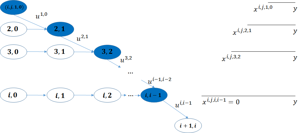
Figure 10.1. Optimal intervention policy summary

Recall that a node is in state $(i,j,c,l)$ if it has in and out degree pair $(i,j)$, sum of initial equity and accumulative interventions $c$ (called total buffer) and number of revealed in links $l$. Similar to Amini et al. (2013), we call the in links to a node that has “distance to default” of one as “contagious” links. So a node in state $(i,j,1,0)$ has $i$ contagious links and a node in state $(i,j,2,1)$ has $i-1$ contagious links and so on, as shown in 10.1 the states in blue color. The insights from the optimal interventions policy are summarized as follows.

1. It is never optimal to intervene on a node if it is not selected or has at least two units of remaining equity when selected. Thus the optimal control policy described in 10.2 only specifies that whether we should intervene on a node that, when selected, has “distance to default” of one, i.e. $l=c-1$. In other words, the use of interventions is to counteract the effects of contagious links.

2. The optimal control policy depends strongly on $K$, the relative cost of interventions. At a higher $K$ value, interventions are costly and the regulator rather lets the contagion to evolve without any interventions, while at a lower $K$ value the regulator implements more and more interventions, even a “complete” intervention strategy, that is, intervening on every selected node with “distance to default” of one since the beginning of the process.

3. The optimal control policy is “monotonic” with respect to the number of out degree of a node. Take $v<0$ for example. There exists a cutoff value of the out degree (specified by $\frac{1-K}{v}$) and it is only optimal to intervene on a node with out degree larger than this cutoff value and not otherwise, regardless of its in degree, total buffer and revealed in links. For nodes with out degree equal to the cutoff value, we have the singular control case that only those with state $(i,j,i,i-1)$—total buffer equal to the in degree and one unit larger than the number of revealed in links—needs interventions and the starting time of interventions is specified by the variable $z$ from the optimization problem (OP).

4. For nodes that are candidates to receive interventions, the starting time of interventions (specified by the definition of $x^{i,j,c,c-1}$) is “monotonic” in terms of the total buffer. The higher the current equity is, the earlier we should begin to intervene as illustrated in 10.1 that $x^{i,j,c,c-1}$ is decreasing in $c$. Moreover, the starting time is also “monotonic” in terms of the in degree and the out degree. Again take $v<0$ for example. The smaller the in degree is or larger the out degree is, the earlier the intervention should begin. So we focus on systematically important nodes and nodes that are close to invulnerability. In other words, we bailout the system by protecting the nodes that would incur large impact on the network after defaulting and by bringing nodes into invulnerable states. Note it is counterintuitive that if there is a positive fraction of the network strongly interlinked by contagious links, we do not prioritize interventions on them unless they have large out degrees.

5. Once we have begun intervening on a node we should keep implementing interventions on it every time it is selected. In other words, we do not allow nodes that have received interventions to default.

Following the optimal policy we are able to achieve earlier termination time of the contagion process and smaller fraction of final defaulted nodes indeed. We can quantify the improvement by comparing $\tilde{I}$ and $\tilde{J}$ in 10.3 with $I$ and $J$ defined in 10.1, respectively. Note in the following we suppress the apostrophe $"*"$ and the indexes $(i,j)$ are in the range $i\lor j<M^{\epsilon}$.

1. $\tilde{I}(y,v,z)$ plays the same role as $I(y)$ in 10.1, which represents the asymptotic scaled total out degree from the default set at scaled time $y$. Since

   $$I(y)-\tilde{I}(y,v,z)$$

   $$=\frac{1}{\lambda}\sum_{i\lor j<M^{\epsilon}}j\{\sum_{c=0}^{i}p(i,j,c)[\mathbb{P}(\text{Bin}(i,y)\geq c)-\mathbb{P}(\text{Bin}(i,x^{i,j,c,c-1})\geq c)]$$

   $$+\mathbbm{1}_{(vj-1=-K)}p(i,j,i)(y^{i}-z^{i})\},$$

   and note that

   (10.3.2) $$x^{i,j,c,c-1}\leq y\text{ for }(i,j,c,c-1)\in\Phi^{\epsilon},$$

   thus

   (10.3.3) $$\mathbb{P}(\text{Bin}(i,y)\geq c)-\mathbb{P}(\text{Bin}(i,x^{i,j,c,c-1})\geq c)\geq 0.$$

   Then for the same initial conditions $p=\left(p(i,j,c)\right)_{i\lor j<M^{\epsilon},0\leq c\leq i}$, the smallest fixed point of $\tilde{I}(y;v^{*},z^{*})$ is no greater than that of $I(y),$ which implies that the default contagion process under optimal interventions terminates no later than under no interventions.

2. Similarly $\tilde{J}(y,v,z)$ plays the same role as $J(y)$ in 10.1, which represents the asymptotic fraction of final defaulted nodes under the optimal control policy. The difference

   $$J(y)-\tilde{J}(y,v,z)$$

   $$= \sum_{i\lor j<M^{\epsilon}}\{\sum_{c=0}^{i}p(i,j,c)[\mathbb{P}(\text{Bin}(i,y)\geq c)-\mathbb{P}(\text{Bin}(i,x^{i,j,c,c-1})\geq c)]$$

   $$+\mathbbm{1}_{(vj-1=-K)}p(i,j,i)(y^{i}-z^{i})\}\geq 0$$

   quantifies the fraction of nodes that are protected from default because of the optimal control policy.

11. Proofs

11.1. Proof of 7.1

Proof.

Assume $u(\tau)=b\coloneqq(b^{\beta})_{\beta\in\Phi}$ for $\tau\in[\tau_{1},\tau_{2})\subseteq[0,\lambda)$, $0\leq\tau_{1}<\tau_{2}<\infty$ and $b^{\beta}\in\{0,1\}$. Note that the ODEs are “separable” in that $s_{\tau}^{i,j,c,l}$ only depends on the entries of $s_{\tau}$ with the same $(i,j)$, so we can only focus on the system of ODEs with the same $(i,j)$. For the same $(i,j)$, define $\Gamma_{i,j}\coloneqq\{(c,l):0\leq l<c\leq i\text{ or }c=i+1,l=i\}$. For simplicity purpose after dropping $i,j$ in the superscripts, we have the set of ODEs for $\tau\in[\tau_{1},\tau_{2})$,

$$\frac{ds_{\tau}^{c,0}}{d\tau} = -\frac{is_{\tau}^{c,0}}{\lambda-\tau}\qquad\text{for $1\leq c\leq i$},$$

$$\frac{ds_{\tau}^{c,l}}{d\tau} = \frac{(i-l+1)s_{\tau}^{c,l-1}}{\lambda-\tau}-\frac{(i-l)s_{\tau}^{c,l}}{\lambda-\tau}$$

$$\text{ for }3\leq c\leq i,1\leq l\leq c-2,$$

$$\frac{ds_{\tau}^{c,c-1}}{d\tau} = \frac{(i-c+2)s_{\tau}^{c-1,c-2}}{\lambda-\tau}b^{c-1,c-2}+\frac{(i-c+2)s_{\tau}^{c,c-2}}{\lambda-\tau}-\frac{(i-c+1)s_{\tau}^{c,c-1}}{\lambda-\tau}$$

$$\text{ for }2\leq c\leq i,$$

$$\frac{ds_{\tau}^{i,j,i+1,i}}{d\tau} = \frac{s_{\tau}^{i,i-1}}{\lambda-\tau}b^{i,i-1},$$

with the initial condition $s_{\tau_{1}}=s_{1}\coloneqq(s_{1}^{c,l})_{(c,l)\in\Gamma_{i,j}}$. Letting $t=-\ln(\lambda-\tau)$, $t_{1}=-\ln(\lambda-\tau_{1})$ and $t_{2}=-\ln(\lambda-\tau_{2})$, we have an autonomous system of ODEs for $t\in[t_{1},t_{2})$ that

(11.1.2) $$\frac{ds_{t}^{c,0}}{dt}=-is_{t}^{c,0}\text{ for }1\leq c\leq i,$$

$$\frac{ds_{t}^{c,l}}{dt}=(i-l+1)s_{t}^{c,l-1}-(i-l)s_{t}^{c,l}$$

(11.1.3) $$\text{ for }3\leq c\leq i,\;1\leq l\leq c-2,$$

$$\frac{ds_{t}^{c,c-1}}{dt}=(i-c+2)s_{t}^{c-1,c-2}b^{c-1,c-2}+(i-c+2)s_{t}^{c,c-2}-(i-c+1)s_{t}^{c,c-1}$$

(11.1.4) $$\text{ for }2\leq c\leq i,$$

(11.1.5) $$\frac{ds_{t}^{i+1,i}}{dt}=s_{t}^{i,i-1}b^{i,i-1},$$

with the initial condition $s_{t_{1}}=s_{1}$.

Lemma 11.1.

Let $s_{t}=(s_{t}^{c,l})_{(c,l)\in\Gamma_{i,j}}$ satisfy the system of ordinary differential equations in (LABEL:eq:AODEPart) with the initial conditions $s_{t_{1}}=s_{1}\coloneqq(s_{1}^{c,l})_{(c,l)\in\Gamma_{i,j}}$in the interval $[t_{1},t_{2})$ and assume $u(t)$ is a constant vector function $u(t)=b\coloneqq(b^{\beta})_{\beta\in\Phi}$ where $b^{\beta}\in\{0,1\}$ on $[t_{1},t_{2})$, then the solution $s_{t}$ on $[t_{1},t_{2})$ is

$$s_{t}^{c,l} =e^{(i-l)(t_{1}-t)}\sum_{r=0}^{l}s_{1}^{c,r}\binom{i-r}{l-r}(1-e^{t_{1}-t})^{l-r}$$

(11.1.6) $$\text{ for }2\leq c\leq i,\;0\leq l\leq c-2,$$

$$s_{t}^{c,c-1} =e^{(i-c+1)(t_{1}-t)}\sum_{r=0}^{c-1}\sum_{q=r+1}^{c}\prod_{k=q}^{c-1}b^{k,k-1}s_{1}^{q,r}\binom{i-r}{c-1-r}(1-e^{t_{1}-t})^{c-1-r}$$

(11.1.7) $$\text{ for }1\leq c\leq i,$$

(11.1.8) $$s_{t}^{i+1,i} =s_{1}^{i+1,i}+\sum_{r=0}^{i-1}\sum_{q=r+1}^{i}\prod_{k=q}^{i}b^{k,k-1}s_{1}^{q,r}(1-e^{t_{1}-t})^{i-r}$$

where $\prod_{k=c}^{c-1}b^{k,k-1}\coloneqq 1$ .

Proof.

We first prove (11.1.6) by induction on $l$ for the same $c$, $2\leq c\leq i$. As the base case $l=0$, (11.1.2) admits the solution that

(11.1.9) $$s_{t}^{c,0}=s_{1}^{c,0}e^{i(t_{0}-t)},$$

which is consistent with (11.1.6). Assume (11.1.6) with $l$ replaced by $l-1$, $1\leq l\leq c-2$ is the solution for (11.1.3), then it follows from (11.1.3) that

$$s_{t}^{c,l} = s_{1}^{c,l}e^{(i-l)(t_{1}-t)}+\int_{t_{1}}^{t}(i-l+1)s_{y}^{c,l-1}e^{(i-l)(y-t)}dy$$

$$= s_{1}^{c,l}e^{(i-l)(t_{1}-t)}+(i-l+1)\int_{t_{1}}^{t}e^{(i-l+1)(t_{1}-y)}e^{(i-l)(y-t)}\sum_{r=0}^{l-1}s_{1}^{c,r}\binom{i-r}{l-1-r}(1-e^{t_{1}-y})^{l-1-r}dy$$

$$= s_{1}^{c,l}e^{(i-l)(t_{1}-t)}+(i-l+1)e^{(i-l)(t_{1}-t)}\sum_{r=0}^{l-1}s_{1}^{c,r}\binom{i-r}{l-1-r}\int_{t_{1}}^{t}e^{t_{1}-y}(1-e^{t_{1}-y})^{l-1-r}dy$$

$$= s_{1}^{c,l}e^{(i-l)(t_{1}-t)}+e^{(i-l)(t_{1}-t)}\sum_{r=0}^{l-1}s_{1}^{c,r}\binom{i-r}{l-1-r}\frac{i-l+1}{l-r}(1-e^{t_{1}-t})^{l-r}$$

$$= s_{1}^{c,l}e^{(i-l)(t_{1}-t)}+e^{(i-l)(t_{1}-t)}\sum_{r=0}^{l-1}s_{1}^{c,r}\binom{i-r}{l-r}(1-e^{t_{1}-t})^{l-r},$$

which is the same as (11.1.6).

For (11.1.7) we prove by induction on $c$, $1\leq c\leq i$. As the base case $c=1$, the solution of (11.1.2) is that

(11.1.11) $$s_{t}^{1,0}=s_{1}^{1,0}e^{i(t_{1}-t)},$$

which is consistent with (11.1.7). Assume (11.1.7) with $c$ replaced by $c-1$, $1\leq c\leq i$ is the solution for (11.1.4), then it follows from (11.1.4) that

(11.1.12) $$s_{t}^{c,c-1} =s_{1}^{c,c-1}e^{(i-c+1)(t_{1}-t)}+(i-c+2)\int_{t_{1}}^{t}(s_{y}^{c-1,c-2}b^{c-1,c-2}+s_{y}^{c,c-2})e^{(i-c+1)(y-t)}dy,$$

where by the induction assumption and (11.1.6) that the second term

$$(i-c+2)\int_{t_{1}}^{t}(s_{y}^{c-1,c-2}b^{c-1,c-2}+s_{y}^{c,c-2})e^{(i-c+1)(y-t)}dy$$

$$= (i-c+2)\int_{t_{1}}^{t}e^{(i-c+1)(y-t)}e^{(i-c+2)(t_{1}-y)}[\sum_{r=0}^{c-2}\sum_{q=r+1}^{c-1}\prod_{k=q}^{c-1}b^{k,k-1}s_{1}^{q,r}\binom{i-r}{c-2-r}(1-e^{t_{1}-y})^{c-2-r}$$

$$+\sum_{r=0}^{c-2}s_{1}^{c,r}\binom{i-r}{c-2-r}(1-e^{t_{1}-y})^{c-2-r}]dy$$

$$= (i-c+2)e^{(i-c+1)(t_{1}-t)}[\sum_{r=0}^{c-2}\sum_{q=r+1}^{c-1}\prod_{k=q}^{c-1}b^{k,k-1}s_{1}^{q,r}\binom{i-r}{c-2-r}\int_{t_{1}}^{t}e^{t_{1}-y}(1-e^{t_{1}-y})^{c-2-r}dy$$

$$+\sum_{r=0}^{c-2}s_{1}^{c,r}\binom{i-r}{c-2-r}\int_{t_{1}}^{t}e^{t_{1}-y}(1-e^{t_{1}-y})^{c-2-r}dy]$$

$$= e^{(i-c+1)(t_{1}-t)}[\sum_{r=0}^{c-2}\sum_{q=r+1}^{c-1}\prod_{k=q}^{c-1}b^{k,k-1}s_{1}^{q,r}\binom{i-r}{c-2-r}\frac{i-c+2}{c-1-r}(1-e^{t_{1}-t})^{c-1-r}$$

$$+\sum_{r=0}^{c-2}s_{1}^{c,r}\binom{i-r}{c-2-r}\frac{i-c+2}{c-1-r}(1-e^{t_{1}-t})^{c-1-r}]$$

$$= e^{(i-c+1)(t_{1}-t)}[\sum_{r=0}^{c-2}\sum_{q=r+1}^{c-1}\prod_{k=q}^{c-1}b^{k,k-1}s_{1}^{q,r}\binom{i-r}{c-1-r}(1-e^{t_{1}-t})^{c-1-r}$$

$$+\sum_{r=0}^{c-2}\prod_{k=c}^{c-1}b^{k,k-1}s_{1}^{c,r}\binom{i-r}{c-1-r}(1-e^{t_{1}-t})^{c-1-r}]$$

$$= e^{(i-c+1)(t_{1}-t)}\sum_{r=0}^{c-2}\sum_{q=r+1}^{c}\prod_{k=q}^{c-1}b^{k,k-1}s_{1}^{q,r}\binom{i-r}{c-1-r}(1-e^{t_{1}-t})^{c-1-r}.$$

Substituting (LABEL:eq:ODESol_Interstep) back into (11.1.12) yields

$$s_{t}^{c,c-1} =s_{1}^{c,c-1}e^{(i-c+1)(t_{1}-t)}+e^{(i-c+1)(t_{1}-t)}\sum_{r=0}^{c-2}\sum_{q=r+1}^{c}\prod_{k=q}^{c-1}b^{k,k-1}s_{1}^{q,r}\binom{i-r}{c-1-r}(1-e^{t_{1}-t})^{c-1-r}$$

$$=e^{(i-c+1)(t_{1}-t)}\sum_{r=0}^{c-1}\sum_{q=r+1}^{c}\prod_{k=q}^{c-1}b^{k,k-1}s_{1}^{q,r}\binom{i-r}{c-1-r}(1-e^{t_{1}-t})^{c-1-r},$$

which proves (11.1.7). Then by (11.1.7) with $c=i$, we have the expression for $s_{t}^{i,i-1}$and (11.1.5) allows the solution that

$$s_{t}^{i+1,i} =s_{1}^{i+1,i}+\int_{t_{1}}^{t}s_{y}^{i,i-1}b^{i,i-1}dy$$

$$=s_{1}^{i+1,i}+\int_{t_{1}}^{t}e^{t_{1}-y}\sum_{r=0}^{i-1}\sum_{q=r+1}^{i}\prod_{k=q}^{i}b^{k,k-1}s_{1}^{q,r}(i-r)(1-e^{t_{1}-y})^{i-1-r}dy$$

$$=s_{1}^{i+1,i}+\sum_{r=0}^{i-1}\sum_{q=r+1}^{i}\prod_{k=q}^{i}b^{k,k-1}s_{1}^{q,r}\int_{t_{1}}^{t}(i-r)e^{t_{1}-y}(1-e^{t_{1}-y})^{i-1-r}dy$$

(11.1.15) $$=s_{1}^{i+1,i}+\sum_{r=0}^{i-1}\sum_{q=r+1}^{i}\prod_{k=q}^{i}b^{k,k-1}s_{1}^{q,r}(1-e^{t_{1}-t})^{i-r},$$

which proves (11.1.8). ∎

By changing the variable $t$ to $\tau$ by $t=-\ln(\lambda-\tau)$, (7.0.2), (7.0.3) and (LABEL:eq:Sol_stau_iplus1i) follow from 11.1. Let the initial condition be $s_{1}^{i,j,c,l}=p(i,j,c)\mathbbm{1}_{(l=0)}$ for $(i,j,c,l)\in\Gamma$ at $\tau_{1}=0$, then (7.0.5) follows. ∎

11.2. Proof of 7.2

Proof.

For the following proof we need to adapt the Wormald’s theorem A.1 in the appendix. For notational convenience we suppress the tilde sign for $\tilde{IT}$, $\tilde{it}$. Since $\frac{m}{n}\rightarrow\lambda$ as $n\rightarrow\infty$, for the given $\epsilon$ and $\hat{\lambda}=\lambda-\epsilon$, we can find $n_{0}\in\mathbb{N}$, such that $0<\hat{\lambda}<\frac{m}{n}<\lambda+0.1$ for $n\geq n_{0}$. Let $z=(z^{\alpha})_{\alpha\in\Gamma^{\epsilon}}$ and

(11.2.1) $$U=\left\{(\tau,z,it)\in\mathbb{R}^{\left|\Gamma^{\epsilon}\right|+2}:\>-\epsilon<\tau<\hat{\lambda},\,-\epsilon<z^{\alpha}<1.1\,,-\epsilon<it<\lambda+0.1\right\},$$

then $U$ contains the closure of

(11.2.2) $$\left\{(0,z,0):\,\mathbb{P}(S_{0}^{\alpha}=z^{\alpha}n,\,\forall\alpha\in\Gamma^{\epsilon},IT_{0}=0)\neq 0\text{ for some }n\right\}.$$

Define the stopping time $T_{U}=\min\{1\leq k\leq m:(\frac{k}{n},\frac{S_{k}}{n},\frac{IT_{k}}{n})\notin U\}$.

By 5.1 and definition of $IT_{k}$, $0\leq S_{k}^{\alpha}\leq n$, $\alpha\in\Gamma^{\epsilon}$ and $0\leq IT_{k}\leq(\lambda+0.1)n$ hold $\forall$$k\geq 0$ and $n\geq n_{0}$. Recall that $S_{k}=(S_{k}^{\alpha})_{\alpha\in\Gamma^{\epsilon}}$ and $\frac{S_{k}}{n}=(\frac{S_{k}^{\alpha}}{n})_{\alpha\in\Gamma^{\epsilon}}$. The following conditions hold:

1. For $0\leq k<T_{U}$ and $\alpha\in\Gamma^{\epsilon}$,

   $$\left|S_{k+1}^{\alpha}-S_{k}^{\alpha}\right| \leq 1,$$

   (11.2.3) $$|IT_{k+1}-IT_{k}| \leq 1,$$

   i.e. $\rho_{1}=1$.

2. There exists $\rho_{2}=O(n^{-1})$ such that for $0\leq k<T_{U}$ and $\alpha\in\Gamma^{\epsilon}$,

   $$\left|\mathbb{E}\left(S_{k+1}^{\alpha}-S_{k}^{\alpha}\mid\mathcal{F}_{k}\right)-h^{\alpha}\left(\frac{k}{n},\frac{S_{k}}{n}\right)\right| \leq\rho_{2},$$

   (11.2.4) $$\left|\mathbb{E}\left(IT_{k+1}-IT_{k}\mid\mathcal{F}_{k}\right)-h_{0}\left(\frac{k}{n},\frac{S_{k}}{n}\right)\right| \leq\rho_{2},$$

   where $h=(h^{\alpha})_{\alpha\in\Gamma^{\epsilon}}$ and $h_{0}$ are

   $$h^{i,j,c,l}\left(t,z\right) =\begin{cases}-\frac{iz^{i,j,c,0}}{\lambda-t}&\text{if }1\leq c\leq i,l=0\\ \frac{(i-l+1)z^{i,j,c,l-1}}{\lambda-t}-\frac{(i-l)z^{i,j,c,l}}{\lambda-t}&\text{if }3\leq c\leq i,1\leq l\leq c-2\\ \frac{(i-c+2)z^{i,j,c-1,c-2}}{\lambda-t}u^{i,j,c-1,c-2}(t)\\ +\frac{(i-c+2)z^{i,j,c,c-2}}{\lambda-t}-\frac{(i-c+1)z^{i,j,c,c-1}}{\lambda-t}&\text{if }2\leq c\leq i\\ \frac{z^{i,j,i,i-1}}{\lambda-t}u^{i,j,i,i-1}(t)&\text{if }c=i,l=i-1\end{cases}$$

   (11.2.5) $$h_{0}(t,z) =\sum_{(i,j,c,c-1)\in\Phi^{\epsilon}}\frac{(i-c+1)z^{i,j,c,c-1}}{\lambda-t}u^{i,j,c,c-1}(t).$$

   In particular, (11.2.4) follows from

   $$\left|\sum_{(i,j,c,c-1)\in\Phi^{\epsilon}}\frac{(i-c+1)S_{k}^{i,j,c,c-1}}{m-k}u^{i,j,c,c-1}(\frac{k}{n})-\sum_{(i,j,c,c-1)\in\Phi^{\epsilon}}\frac{(i-c+1)\frac{S_{k}^{i,j,c,c-1}}{n}}{\lambda-\frac{k}{n}}u^{i,j,c,c-1}(\frac{k}{n})\right|$$

   $$\leq \sum_{(i,j,c,c-1)\in\Phi^{\epsilon}}\left|\frac{(i-c+1)\frac{S_{k}^{i,j,c,c-1}}{n}}{\frac{m}{n}-\frac{k}{n}}u^{i,j,c,c-1}(\frac{k}{n})-\frac{(i-c+1)\frac{S_{k}^{i,j,c,c-1}}{n}}{\lambda-\frac{k}{n}}u^{i,j,c,c-1}(\frac{k}{n})\right|$$

   $$= O(n^{-1}).$$

However, for $\beta\in\Phi^{\epsilon}$, $h^{\beta}$ and $h_{0}$ are not Lipschitz continuous because $u^{\beta}(\tau)$ can have step changes on $[0,\lambda)$. So we need to adapt the proof. Note that $u^{\beta}(\tau)$ is piecewise constant $\{0,1\}$ valued function thus $h^{\beta}(\tau,s)$ and $h_{0}(\tau,s)$ are Lipschitz continuous in each interval where $\tilde{u}=(u^{\beta})_{\beta\in\Phi^{\epsilon}}$ is a constant vector and then we can apply A.1. In the following define $s_{\tau}(\tau^{\prime},x)$ as the solution of the ODEs,

(11.2.7) $$\frac{d}{d\tau}s_{\tau} =h(\tau,s_{\tau}),$$

which are understood as for $\alpha\in\Gamma^{\epsilon}$,

(11.2.8) $$\frac{d}{d\tau}s_{\tau}^{\alpha}=h^{\alpha}(\tau,s_{\tau}),$$

with initial condition at $\tau^{\prime}$, $s_{\tau^{\prime}}=x\coloneqq(x^{\alpha})_{\alpha\in\Gamma^{\epsilon}}$.

In what follows define the points where any component of $\tilde{u}(\tau)$ has a step change. $\tau_{l}\coloneqq\inf\{\tau>\tau_{l-1}:u^{\beta}(\tau)\text{ has a step change for some }\beta\in\Phi^{\epsilon}\}\land\hat{\lambda}$ for $l\geq 1$ and $\tau_{0}\coloneqq 0$. Also let $k_{l}=\left\lceil n\tau_{l}\right\rceil$, where $\left\lceil\cdot\right\rceil$ is the ceiling function. As a result, $k_{l}-1<n\tau_{l}\leq k_{l}$. Recall the initial condition $s_{0}=(s_{0}^{\alpha})_{\alpha\in\Gamma^{\epsilon}}$ with $s_{0}^{i,j,c,l}=p(i,j,c)\mathbbm{1}_{(l=0)}$. Because every $u^{\beta}$ for $\beta\in\Phi^{\epsilon}$ has only a finite number of step changes on $[0,\lambda)$ and on the other hand $\Phi^{\epsilon}$ is a finite set, there are in total a finite number of step changes for all the functions in $\tilde{u}$ on $[0,\lambda)$.

Then by A.1, let $\rho=n^{-\frac{1}{4}}$, it follows that

(11.2.9) $$\sup_{0\leq k\leq k_{1}-1}\frac{S_{k}^{\alpha}}{n}-s_{\frac{k}{n}}^{\alpha}(0,s_{0})=O(n^{-\frac{1}{4}})$$

with probability $1-O(n^{\frac{1}{4}}\exp(-n^{\frac{1}{4}}))$, $\forall\>\alpha\in\Gamma^{\epsilon}$. Note that we will write “with probability $1-O(n^{\frac{1}{4}}\exp(-n^{\frac{1}{4}}))$” as whp hereinafter.

In particular, we have that

(11.2.10) $$\frac{S_{k_{1}-1}^{\alpha}}{n}-s_{\frac{k_{1}-1}{n}}^{\alpha}(0,s_{0})=O(n^{-\frac{1}{4}})\;\text{ whp.}$$

Additionally by A.1 again we have that

(11.2.11) $$\sup_{k_{1}\leq k\leq k_{2}-1}\frac{S_{k}^{\alpha}}{n}-s_{\frac{k}{n}}^{\alpha}(\frac{k_{1}}{n},\frac{S_{k_{1}}}{n})=O(n^{-\frac{1}{4}})\;\text{ whp.}$$

Note that

(11.2.12) $$\left|\frac{S_{k_{1}}^{\alpha}}{n}-\frac{S_{k_{1}-1}^{\alpha}}{n}\right|\leq\frac{1}{n}\,\forall\alpha\in\Gamma^{\epsilon},$$

and by the Lipschitz continuity of $s_{\tau}^{\alpha}(0,s_{0})$ on $(0,\tau_{1}^{-})$,

(11.2.13) $$s_{\frac{k_{1}-1}{n}}^{\alpha}(0,s_{0})-s_{\tau_{1}}^{\alpha}(0,s_{0})=O(n^{-1}).$$

So by (11.2.10), (11.2.12) and (11.2.13), we have

$$\left|\frac{S_{k_{1}}^{\alpha}}{n}-s_{\tau_{1}}^{\alpha}(0,s_{0})\right| \leq\left|\frac{S_{k_{1}}^{\alpha}}{n}-\frac{S_{k_{1}-1}^{\alpha}}{n}\right|+\left|\frac{S_{k_{1}-1}^{\alpha}}{n}-s_{\frac{k_{1}-1}{n}}^{\alpha}(0,s_{0})\right|$$

$$+\left|s_{\frac{k_{1}-1}{n}}^{\alpha}(0,s_{0})-s_{\tau_{1}}^{\alpha}(0,s_{0})\right|$$

(11.2.14) $$=n^{-1}+O(n^{-\frac{1}{4}})+O(n^{-1})\;\text{ whp.}$$

Thus we have that

(11.2.15) $$\left\|\frac{S_{k_{1}}}{n}-s_{\tau_{1}}(0,s_{0})\right\|=O(n^{-\frac{1}{4}})+O(n^{-1})\;\text{ whp.}$$

where $\left\|\eta\right\|$ is the norm for $\eta\in\mathbb{R}^{|\Gamma^{\epsilon}|}$.

From 7.1 we see that the derivative of $s_{\tau}^{\alpha}$ with respect to the initial time and initial condition is bounded for $\tau_{1}<\tau<\hat{\lambda}<\lambda$, i.e.

(11.2.16) $$\left\|\frac{\partial s_{\tau}^{\alpha}(\tau^{\prime},x)}{\partial(\tau^{\prime},x)}\right\|\leq M_{1}<\infty$$

where $M_{1}$ is a constant. Recall that $|\frac{k_{1}}{n}-\tau_{1}|<n^{-1}$, so by (11.2.14) and (11.2.16), it follows that

$$s_{\tau}^{\alpha}(\frac{k_{1}}{n},\frac{S_{k_{1}}}{n})-s_{\tau}^{\alpha}(\tau_{1},s_{\tau_{1}}(0,s_{0}))$$

$$=s_{\tau}^{\alpha}(\frac{k_{1}}{n},\frac{S_{k_{1}}}{n})-s_{\tau}^{\alpha}(0,s_{0})$$

(11.2.17) $$=O(n^{-\frac{1}{4}})+O(n^{-1})\text{\; whp},$$

for $\tau\in(\tau_{1},\tau_{2})$. So it follows that

(11.2.18) $$\sup_{k_{1}\leq k\leq k_{2}-1}\frac{S_{k}^{\alpha}}{n}-s_{\frac{k}{n}}^{\alpha}(0,s_{0})=O(n^{-\frac{1}{4}})\;\text{ whp.}$$

Similarly for $IT_{k}$, define $it_{\tau}(\tau^{\prime},x,y)$ as the solution of

(11.2.19) $$\frac{d}{d\tau}it_{\tau}=h_{0}(\tau,s_{\tau}),$$

with the initial condition at $\tau^{\prime}$, $(s_{\tau^{\prime}},it_{\tau^{\prime}})=(x,y)$. Applying A.1 for $IT_{k}$ and $it_{\tau}$ gives that,

$$\sup_{0\leq k\leq k_{1}-1}\frac{IT_{k}}{n}-it_{\frac{k}{n}}(0,s_{0},0) =O(n^{-\frac{1}{4}})\;\text{ whp},$$

(11.2.20) $$\sup_{k_{1}\leq k\leq k_{2}-1}\frac{IT_{k}}{n}-it_{\frac{k}{n}}(\frac{k_{1}}{n},\frac{S_{k_{1}}}{n},\frac{IT_{k_{1}}}{n}) =O(n^{-\frac{1}{4}})\;\text{ whp}.$$

In particular,

(11.2.21) $$\frac{IT_{k_{1}-1}}{n}-it_{\frac{k_{1}-1}{n}}(0,s_{0},0)=O(n^{-\frac{1}{4}})\;\text{ whp},$$

Further note that

(11.2.22) $$\left|\frac{IT_{k_{1}}}{n}-\frac{IT_{k_{1}-1}}{n}\right|\leq\frac{1}{n}\,\forall\alpha\in\Gamma^{\epsilon},$$

and by the Lipschitz continuity of $it_{\tau}(0,s_{0},0)$ on $(0,\tau_{1}^{-})$,

(11.2.23) $$it_{\frac{k_{1}-1}{n}}(0,s_{0},0)-it_{\tau_{1}}(0,s_{0},0)=O(n^{-1}).$$

So by (11.2.21), (11.2.22) and (11.2.23) we have

$$\left|\frac{IT_{k_{1}}}{n}-it_{\tau_{1}}(0,s_{0},0)\right| \leq\left|\frac{IT_{k_{1}}}{n}-\frac{IT_{k_{1}-1}}{n}\right|+\left|\frac{IT_{k_{1}-1}}{n}-it_{\frac{k_{1}-1}{n}}(0,s_{0},0)\right|$$

$$+\left|it_{\frac{k_{1}-1}{n}}(0,s_{0},0)-it_{\tau_{1}}(0,s_{0},0)\right|$$

(11.2.24) $$=n^{-1}+O(n^{-\frac{1}{4}})+O(n^{-1})\;\text{ whp.}$$

Recall we have proved in (11.2.14) that

(11.2.25) $$\left|\frac{S_{k_{1}}^{\alpha}}{n}-s_{\tau_{1}}^{\alpha}(0,s_{0})\right|\leq O(n^{-\frac{1}{4}})+O(n^{-1})\text{\; whp}.$$

Here we apply the fact we shall prove later that the derivative of $it_{\tau}$ with respect to the initial time and initial condition is bounded for $\tau$ in an interval on which $\tilde{u}$ is a constant vector function and $\tau<\hat{\lambda}$, i.e.

(11.2.26) $$\left\|\frac{\partial it_{\tau}(\tau^{\prime},x,y)}{\partial(\tau^{\prime},x,y)}\right\|\leq M_{2}<\infty$$

for some constant $M_{2}$. Recall that $|\frac{k_{1}}{n}-\tau_{1}|<n^{-1}$, so by (11.2.24), (11.2.25) and (11.2.26), we have that

$$it_{\tau}(\frac{k_{1}}{n},\frac{S_{k_{1}}}{n},\frac{IT_{k_{1}}}{n})-it_{\tau}(\tau_{1},s_{\tau_{1}}(0,s_{0}),it_{\tau_{1}}(0,s_{0},0))$$

$$=it_{\tau}(\frac{k_{1}}{n},\frac{S_{k_{1}}}{n},\frac{IT_{k_{1}}}{n})-it_{\tau}(0,s_{0},0)$$

(11.2.27) $$=O(n^{-\frac{1}{4}})+O(n^{-1})\text{\; whp},$$

for $\tau\in(\tau_{1},\tau_{2})$. So it follows that

(11.2.28) $$\sup_{k_{1}\leq k\leq k_{2}-1}\frac{IT_{k}}{n}-it_{\frac{k}{n}}(0,s_{0},0)=O(n^{-\frac{1}{4}})\;\text{ whp.}$$

We can repeat the above procedure every time any $u^{\beta}(\tau)$ has a step change, $\beta\in\Phi^{\epsilon}$ and there are only a finite number of step changes in $[0,\lambda)$. Because $s_{\tau}^{\alpha}\leq 1$ and $it_{\tau}\leq\lambda$, $d_{\infty}\left((s_{\tau},it_{\tau}),\partial U\right)\geq 0.1\geq Cn^{-\frac{1}{4}}$, for a sufficiently large constant $C$. Thus the supremum of $\tau$ that $(s_{\tau},it_{\tau})$ can be extended to the boundary of $U$ is $\hat{\lambda}$, i.e. in (A.0.9) of A.1,

$$\sigma =\sup\left\{\tau\geq 0:\,d_{\infty}\left((s_{\tau},it_{\tau}),\partial U\right)\geq Cn^{-\frac{1}{4}}\right\}$$

$$=\hat{\lambda}.$$

So it follows that

$$\sup_{0\leq k\leq n\hat{\lambda}}\frac{S_{k}^{\alpha}}{n}-s_{\frac{k}{n}}^{\alpha}(0,s_{0}) =O(n^{-\frac{1}{4}})\;\text{ whp},$$

(11.2.29) $$\sup_{0\leq k\leq n\hat{\lambda}}\frac{IT_{k}}{n}-it_{\frac{k}{n}}(0,s_{0},0) =O(n^{-\frac{1}{4}})\;\text{ whp.}$$

At last we prove that the derivative of $it_{\tau}$ with respect to the initial time and initial condition is bounded as in (11.2.26). Note first that $it_{\tau}$ with initial condition $\bar{s}=(s_{\tau^{\prime}},it_{\tau^{\prime}})$ at $\tau=\tau^{\prime}$ in an interval where $\tilde{u}$ is a constant vector function $b=(b^{\beta})_{\beta\in\Phi^{\epsilon}}$ satisfies that

(11.2.30) $$it_{\tau}=it_{\tau^{\prime}}+\int_{\tau^{\prime}}^{\tau}\sum_{(i,j,c,c-1)\in\Phi^{\epsilon}}\frac{(i-c+1)b^{i,j,c,c-1}}{\lambda-u}s_{u}^{i,j,c,c-1}(\tau^{\prime},s_{\tau^{\prime}})du.$$

First we show that the derivative of $it_{\tau}$ with respect to the initial condition $\bar{s}$ is bounded.

(11.2.31) $$\frac{\partial it_{\tau}}{\partial\bar{s}}=e^{\text{last}}+\int_{\tau^{\prime}}^{\tau}\sum_{(i,j,c,c-1)\in\Phi^{\epsilon}}\frac{(i-c+1)b^{i,j,c,c-1}}{\lambda-u}\frac{\partial s_{u}^{i,j,c,c-1}(\tau^{\prime},s_{\tau^{\prime}})}{\partial\bar{s}}du$$

where $e^{\text{last}}$ is a vector of zeros except an entry of one at the last. Thus

(11.2.32) $$\left\|\frac{\partial it_{\tau}}{\partial\bar{s}}\right\|\leq 1+\int_{\tau^{\prime}}^{\tau}\sum_{(i,j,c,c-1)\in\Phi^{\epsilon}}\frac{(i-c+1)b^{i,j,c,c-1}}{\lambda-u}\left\|\frac{\partial s_{u}^{i,j,c,c-1}(\tau^{\prime},s_{\tau^{\prime}})}{\partial\bar{s}}\right\|du.$$

By (11.2.16), $\left\|\frac{\partial s_{u}^{i,j,c,c-1}}{\partial\bar{s}}\right\|<M_{1}$ and thus $\left\|\frac{\partial it_{\tau}}{\partial\bar{s}}\right\|$ is bounded for $\tau<\hat{\lambda}$. Next we show that the derivative of $it_{\tau}$ with respect to the initial time $\tau^{\prime}$ is bounded. By the Leibniz integral rule, we have

$$\frac{\partial it_{\tau}}{\partial\tau^{\prime}} =-\sum_{(i,j,c,c-1)\in\Phi^{\epsilon}}\frac{(i-c+1)b^{i,j,c,c-1}}{\lambda-\tau^{\prime}}s_{\tau^{\prime}}^{i,j,c,c-1}(\tau^{\prime},s_{\tau^{\prime}})$$

(11.2.33) $$+\int_{\tau^{\prime}}^{\tau}\sum_{(i,j,c,c-1)\in\Phi^{\epsilon}}\frac{(i-c+1)b^{i,j,c,c-1}}{\lambda-u}\frac{\partial s_{u}^{i,j,c,c-1}(\tau^{\prime},s_{\tau^{\prime}})}{\partial\tau^{\prime}}du,$$

where $s_{\tau^{\prime}}^{i,j,c,c-1}(\tau^{\prime},s_{\tau^{\prime}})=s_{\tau^{\prime}}^{i,j,c,c-1}$. Since by (11.2.16), $\left|\frac{\partial s_{u}^{i,j,c,c-1}(\tau^{\prime},s_{\tau^{\prime}})}{\partial\tau^{\prime}}\right|$ is bounded thus $\left|\frac{\partial it_{\tau}}{\partial\tau^{\prime}}\right|$ is bounded for $\tau<\hat{\lambda}$. Thus we proved (11.2.26). ∎

11.3. Proof of 10.1

Proof.

For the contagion process without intervention, we relate our model to the auxiliary model used in the proof in Amini et al. (2013).

Recall that in 4.2 we are given a set of nodes $[n]$ and the sequence of degrees $(d^{-}(v),d^{+}(v))_{v\in[n]}$ as well as the initial equity levels $\left(e_{0}^{v}\right)_{v\in[n]}$. For each node $v$ we assign each in stub a number ranging in $\{1,\ldots,d^{-}(v)\}$. Let $\Sigma^{v}$ be the set of all permutations of the in stubs of node $v\in[n]$, then a permutation $\tau\in\Sigma^{v}$ specifies the order in which $v$ receives shocks through the in stubs.

Because every in stub of $v$ represents one unit of loan, $v$ will default after $e_{0}^{v}$ of its in stubs have been connected (or $e_{0}^{v}$ of its in links have been revealed) for every permutation $\tau\in\Sigma^{v}$. In other words, if we define $\theta(v,\tau)$ to be the number of shocks that $v$ can sustain if the order in which the in stubs are connected is specified by $\tau$, then it follows that $\theta(v,\tau)=e_{0},\forall\tau\in\Sigma^{v}$ and

$$\frac{\left|\{(v,\tau)\mid v\in[n],\tau\in\Sigma^{v},d^{-}(v)=i,d^{+}(v)=j,\theta(v,\tau)=c\}\right|}{n\mu(i,j)i!}$$

$$= \frac{\left|\{v\mid v\in[n],\tau\in\Sigma^{v},d^{-}(v)=i,d^{+}(v)=j,e_{0}^{v}=c\}\right|}{n\mu(i,j)}$$

(11.3.1) $$= \sigma(i,j,c).$$

Then 1 satisfies the assumption $4.1$ and $4.2$ in Amini et al. (2013). Moreover, under no intervention, the random graph generated in 4.2 conforms to the model defined in definition $5.4$ in Amini et al. (2013) with in and out degree sequences $(d^{-}(v),d^{+}(v))_{v\in[n]}$ and default thresholds $\left(e_{0}^{v}\right)_{v\in[n]}$. So by their theorem $3.8$ we achieve the conclusions of 10.1. ∎

11.4. Proof of 10.2

Proof.

To simplify the notations we suppress the apostrophe $"*"$. In 9.1 we have presented the optimal control policy $(u_{t})_{t\in[t_{0},t_{f}]}$ in terms of $t$,$t_{0}$,$t_{f}$,$t_{s}$,$t^{i,j,c}$. Recall that in (LABEL:eq:x_and_xijc) we have the following relations,

$$t = -\ln(\lambda-\tau),$$

$$t_{0} = -\ln\lambda,$$

$$y = 1-e^{t_{0}-t_{f}},$$

$$z = 1-e^{t_{0}-t_{s}},$$

$$x^{i,j,c,c-1} = 1-e^{t_{0}-t^{i,j,c}}$$

$$= \begin{cases}y&\text{if }K+vj-1\geq 0\text{ or }c=0\\ 1-(1-y)\frac{(i-c)K}{(i-c+1)K+vj-1}&\text{if }K+vj-1<0\text{ and }1\leq c<i+\frac{K+vj-1}{Ky}\\ 0&\text{otherwise},\end{cases}$$

so we can change the variable from $t$ to $\tau$. Particularly we apply mapping $f(t)=1-e^{t_{0}-t}$ which is a strictly increasing function in $t$, then we have the following correspondences:

Variable	After mapping $1-e^{t_{0}-t}$
$t$	$\frac{\tau}{\lambda}$
$t_{0}$	$0$
$t^{i,j,c}$	$x^{i,j,c,c-1}$
$t_{s}$	$z$
$t_{f}$	$y$

Table 2. Correspondence of variables through mapping $1-e^{t_{0}-t}$.

We replace each variable $t$,$t_{0}$,$t_{f}$,$t_{s}$,$t^{i,j,c}$ in 9.1 with its corresponding variable in 2 resulting in the expressions for $u_{\tau}^{i,j,c,c-1}$. At last by 2 on the relations between the control policy $G_{n}=(g_{1}^{(n)},\ldots,g_{m}^{(n)})$ and the function $u$, we have the conclusion in 10.2. ∎

11.5. Proof of 10.3

Proof.

By the definition of $\tilde{I}(y;v,z)$ and $\tilde{J}(y;v,z)$ in (10.2.1), $d_{\tau_{f}}^{-}$ and $d_{\tau_{f}}$ with $i\lor j<M^{\epsilon}$ in (LABEL:eq:EqOfdWithInt) at $\tau=\tau_{f}$ becomes

$$d_{\tau_{f}}^{-} =\sum_{i\lor j<M^{\epsilon}}j\left[\sum_{c=0}^{i}p(i,j,c)\mathbb{P}(\text{Bin}(i,x^{i,j,c,c-1})\geq c)\right.$$

$$\left.-\mathbbm{1}_{(vj-1=-K)}p(i,j,i)\left((\frac{\tau_{f}}{\lambda})^{i}-z^{i}\right)\right]-\tau_{f}$$

$$=\lambda\left(\tilde{I}(\frac{\tau_{f}}{\lambda};v,z)-\frac{\tau_{f}}{\lambda}\right)$$

$$d_{\tau_{f}} =\sum_{i\lor j<M^{\epsilon}}\left[\sum_{c=0}^{i}p(i,j,c)\mathbb{P}(\text{Bin}(i,x^{i,j,c,c-1})\geq c)\right.$$

$$\left.-\mathbbm{1}_{(vj-1=-K)}p(i,j,i)\left((\frac{\tau_{f}}{\lambda})^{i}-z^{i}\right)\right]$$

(11.5.1) $$=\tilde{J}(\frac{\tau_{f}}{\lambda};v,z).$$

Suppose $(y^{*},v^{*},z^{*})$ is an optimal solution for the optimization problem (OP) and note that $y^{*}$ is the fixed point of $\tilde{I}(y;v^{*},z^{*})$ and $y^{*}=\frac{\tau_{f}^{*}}{\lambda}$.

1. If $y^{*}=1$, then $\tau_{f}^{*}=\lambda$. By the definition of $d_{\tau_{f}}^{-}$, it can only occur when $\sum_{i\lor j<M^{\epsilon}}j\sum_{c=0}^{i}p(i,j,c)=\lambda$ and $z^{*}=\frac{\tau_{f}^{*}}{\lambda}=1$, thus we have $d_{\tau_{f}^{*}}=d_{\lambda}=1$, then by 7.4,

   (11.5.2) $$\frac{D_{n}}{n}\overset{p}{\rightarrow}1,$$

   which proves (1) of 10.3.

2. If $y^{*}<1$ and $\tilde{I}^{\prime}(y^{*};v^{*},z^{*})<1$, then $\tau_{f}^{*}<\lambda$ and $\frac{d}{d\tau}d_{\tau_{f}^{*}}^{-}=\tilde{I}^{\prime}(\frac{\tau_{f}^{*}}{\lambda};v^{*},z^{*})-1<0$. Again it follows from 7.4,

   (11.5.3) $$\frac{D_{n}}{n}\overset{p}{\rightarrow}d_{\tau_{f}^{*}}=\tilde{J}(y^{*};v^{*},z^{*}).$$

   which proves (2) of 10.3. This concludes the proof of 10.3.

It is important to note that the two cases in 10.3 corresponds to $\tau_{f}^{*}=\lambda$, and $\tau_{f}^{*}<\lambda$, $\frac{d}{d\tau}d_{\tau_{f}^{*}}^{-}<0$, respectively. By 7.4 they guarantees that the limits of $\mathbb{E}\frac{IT_{n}(G_{n},P_{n})}{n}$ and $\mathbb{E}\frac{D_{n}(G_{n},P_{n})}{n}$ in (ACP) as $n\rightarrow\infty$ are well defined, which are $it_{\tau_{f}}$ and $d_{\tau_{f}}$, respectively. ∎

Part IV Numerical Experiments

12. Introduction

Consider a sequence of networks with the number of nodes $n$ growing to infinity, whose in and out degrees are between 1 and 10, and each node’s in degree equal to its own out degree, i.e. $d^{-}(v)=d^{+}(v)$, $v\in[n]$, respectively, so we call either the in or out degree as the degree of the node. This allows us to combine two indexes $i$ and $j$ into one index $i$, so the state of a node becomes $(i,c,l)$ and the empirical probability $P_{n}$ and the limiting probability $p$ of the degree and initial equity become $P_{n}(i,c)$ and $p(i,c)$ for $(i,c)\in\Gamma^{{}^{\prime}}\coloneqq\{(i,c)\in\mathbb{N}_{0}^{2}:1\leq i\leq 10,0\leq c\leq 10\}$.

Next we decide on the limiting probability $p$. Note that $\Gamma^{{}^{\prime}}$ contains three initial types of nodes: defaulted (with $c=0$), vulnerable (with $c\leq i$) and invulnerable (with $c>i$). In this numerical experiment, we set the total fraction of initial defaults as $\xi$ and assume the fraction of initial defaults is the same across all degrees, i.e. $p(i,0)=\frac{\xi}{10}$ for $i\in[1,10]$. For the initially liquid nodes, the joint probability of the degree and initial equity conditional on being liquid is constructed through a binormal copula with correlation $\rho$ and two marginal probabilities. The marginal probabilities of the degree and initial equity are assumed to follow the Zipf’s law, i.e.

$$\mathbb{P}(\text{deg}=i) = \frac{i^{-(1+a_{1})}}{\sum_{i=1}^{10}i^{-(1+a_{1})}}$$

$$\mathbb{P}(\text{initial equity}=c) = \frac{c^{-(1+a_{2})}}{\sum_{i=1}^{10}c^{-(1+a_{2})}},$$

where $a_{1},a_{2}>0$. The Zipf’s law is a form of the power law with Pareto tails, which is observed for the distribution of the degrees and equity levels of the financial networks in many empirical studies, see e.g. Boss and Elsinger (2004); Bech and Atalay (2010).

In a network of size $n$ with the joint probability $P_{n}(i,c)$ of the degree and initial equity, a contagion process under interventions occurs as described in 4.2. Recall that we only need to consider intervening on a node that, when selected, has only one unit of equity left, i.e. a node with “distance to default” equal to one. Here we consider two types of intervention policies, the optimal policy and the alternative policy: intervening on nodes with degree between 8 and 10 and “distance to default” equal to one from the beginning of the process. The alternative policy is usually the one adopted by the central bank or government in a real financial crisis setting.

Our objective is to verify the convergence in probability of $\frac{IT_{n}}{n}$ and $\frac{D_{n}}{n}$ as well as the convergence of the scaled termination time $\frac{T_{n}}{m}$ as stated in 7.4. Moreover, we shall study the convergence rate of the standard deviation and IQR (interquartile range) to examine if the asymptotic variables provide good approximations to realistic $n$ values.

Under the optimal policy in the form given in 10.2, the limits for $\frac{IT_{n}}{n}$, $\frac{D_{n}}{n}$ and $\frac{T_{n}}{m}$ as $n\rightarrow\infty$ are $it(y^{*},v^{*},z^{*})$, $\tilde{J}(y^{*},v^{*},z^{*})$ and $y^{*}$, respectively in (OP) where $(y^{*},v^{*},z^{*})$ is the optimal solution. On the other hand, the alternative policy is that for $0\leq k\leq m-1$,

(12.0.2) $$g_{k+1}^{(n),\text{alt}}(s,w)=\begin{cases}\mathbbm{1}_{(k\geq n\lambda x_{\text{alt}}^{i,c,c-1})}&\text{if }w=(i,c,c-1)\in\Phi^{\prime}\\ 0&\text{otherwise},\end{cases}$$

where for $(i,c,c-1)\in\Phi^{\prime}$,

(12.0.3) $$x_{\text{alt}}^{i,c,c-1}=\begin{cases}0&\text{ if }i\in\{8,9,10\}\\ y&\text{otherwise}.\end{cases}$$

Then the limits for $\frac{IT_{n}}{n}$, $\frac{D_{n}}{n}$ and $\frac{T_{n}}{m}$ as $n\rightarrow\infty$ can be calculated as:

$$\frac{IT_{n}}{n}\overset{p}{\to}$$

$$\sum_{i=0}^{10}\sum_{c=1}^{i}p(i,c)\sum_{m=c}^{i}\sum_{n=0}^{c-1}(m-c+1)\mathbb{P}(\text{Multin}(i,x_{\text{alt}}^{i,c,c-1},y-x_{\text{alt}}^{i,c,c-1},1-y)=(n,m-n,i-m)),$$

$$\frac{D_{n}}{n}\overset{p}{\to}\sum_{i=0}^{10}\sum_{c=0}^{i}p(i,c)\mathbb{P}(\text{Bin}(i,x_{\text{alt}}^{i,c,c-1})\geq c),$$

$$\frac{T_{n}}{m}\overset{p}{\to}y$$

where $y$ is the solution of $\frac{1}{\lambda}\sum_{i=0}^{10}i\sum_{c=0}^{i}p(i,c)\mathbb{P}(\text{Bin}(i,x_{\text{alt}}^{i,c,c-1})\geq c)=y$, and $\mathbb{P}(\text{Bin}(i,y)\geq c)=\sum_{m=c}^{i}\binom{i}{m}y^{m}(1-y)^{i-m}$ , $\mathbb{P}(\text{Multin}(i,x,y,1-x-y)=(a,b,i-a-b))=\binom{i}{a,b,i-a-b}x^{a}y^{b}(1-x-y)^{i-a-b}$.

13. Simulation

13.1. The set up

We have the following setup.

1. A sequence of six networks with increasing number of nodes $n\in\{5^{4},6^{4},\ldots,10^{4}\}$ and there are 100 runs for each network under each intervention policy.

2. To determine the asymptotic fraction $p(\cdot,\cdot)$ of the degree and initial equity pair $(i,c)$ where $(i,c)\in\Gamma^{{}^{\prime}}$, we set the following parameters.

   1. The fraction of initial defaults $\xi=0.5$, indicating half of the nodes have defaulted. We assume in this numerical experiment that the fraction of initial defaults is the same across all degrees, thus $p(i,0)=\frac{\xi}{10}$ for $i\in[1,10]$.

   2. The conditional probability of the degree and initial equity for liquid nodes $p(i,e)$, $i\in\{1,\ldots,10\}$, $e\in\{1,\ldots,10\}$ is determined by a binormal coupula with the exponents of the marginal probabilities of the degree and initial equity $(a_{1},a_{2})=(0.8,0.7)$ and the correlation coefficient $\rho=0.9$. Note that a smaller $a_{1}$ indicates larger fraction of nodes with higher degrees, thus higher connectivity and a smaller $a_{2}$ indicates larger fraction of nodes with higher initial equities, and $\rho$ implies how likely that higher degree nodes have higher initial equities.

3. After determining the asymptotic fraction $p(\cdot,\cdot)$, we construct a sequence of empirical fractions $P_{n}(\cdot,\cdot)$ for each network that converge to $p(\cdot,\cdot)$ by

   (13.1.1) $$P_{n}(i,c)=\frac{[np(i,c)]}{n}\qquad(i,c)\in\Gamma^{{}^{\prime}},$$

   where $[\cdot]$ is the round function. In other words, the number of nodes with degree $i$ and initial equity $c$ are $[np(i,c)]$ for a network of $n$ nodes.

4. We consider two intervention policies described as before.

5. The relative cost for the interventions $K=0.5$.

13.2. Simulation results

In the following we suppress the $n$ in the subscripts. We show the plots for $\frac{IT}{n}$, $\frac{D}{n}$ and $\frac{T}{m}$ under the optimal and alternative policies.

1. Under either policy and for each variable, there are four plots in each figure. The first two plots are two boxplots. The above boxplot visualizes five summary statistics (min, mean$-$standard deviation, mean, mean$+$standard deviation, max) while the bottom boxplot uses a another set of summary statistics (1st quartile$-$1.5IQR,1st quartile, median, 3rd quartile, 3rd quartile$+$1.5IQR) and the data outside the range are treated as outliers, where IQR stands for interquartile range, i.e. the difference between the third and the first quartiles.

2. The blue dashed horizontal line in each plot indicates the theoretical values for the limits of $\frac{IT}{n}$, $\frac{D}{n}$ and $\frac{T}{m}$ with $p(\cdot,\cdot)$ and the red solid line in each box indicates those values calculated with $P_{n}(\cdot,\cdot)$ for each $n$. We calculate the theoretical values in both ways because for small $n$, $P_{n}(\cdot,\cdot)$ determined by (13.1.1) has a relatively large rounding error and thus deviates from $p(\cdot,\cdot)$. Calculating using $P_{n}(\cdot,\cdot)$ instead of $p(\cdot,\cdot)$ can effectively remove the deviations in the inputs to the model. Moreover, $P_{n}(\cdot,\cdot)$ is different for different $n$ values, thus the theoretical values of a variable calculated with $P_{n}(\cdot,\cdot)$ are also different for different $n$’s.

3. The black dots in the boxplots indicates the results of 100 runs and they are jittered by a random amount left and right to avoid overplotting. From the black dots we can see the distributions of the results. Note that the black dots in the above and bottom boxplots show the same results for the same $n$. They look different because they are jittered by a different random amount.

4. The last two plots in every figure shows the log-log plot of the standard deviation and IQR of $\frac{IT}{n}$, $\frac{D}{n}$ and $\frac{T}{m}$ against $n$ and a fitted straight line with the slope.

From the simulation results, we make the following conclusions.

1. From the boxplots of $\frac{IT}{n}$, $\frac{D}{n}$ and $\frac{T}{m}$ under both interventions policies, we observe that the mean or median converge to the calculated theoretical value with shrinking standard deviation or IQR. Because the theoretical value is a constant given the joint probability of degree and initial equity $p(\cdot,\cdot)$, convergence of mean to the theoretical value with variance converging to zero is equivalent to convergence in probability, this observation provides evidence for the convergences in probability of $\frac{IT}{n}$, $\frac{D}{n}$ and $\frac{T}{m}$ to their theoretical values.

2. Be comparing the blue dashed line and the red solid line we see that the mean or median is closer to the red solid line, i.e. the theoretical value calculated with $P_{n}(\cdot,\cdot)$ instead of $p(\cdot,\cdot)$. This reflects the rounding error caused by (13.1.1) in the inputs into the calculation. By using the more accurate fraction we observe that the closeness of the mean or median to the theoretical value does not vary in $n$ although the results of different runs are more and more concentrated around the mean or median as $n$ grows.

3. The log-log plots of the standard deviation and IQR of each variable with the fitted straight lines further show that both of them decrease with power law tails, i.e. in the form of $z=Cx^{-a}$ where $C$ is a constant and $a>0$ is the exponent. The absolute value of the slope of the straight line serves as the exponent. It is interesting to observe that the exponents for the standard deviation and IQR are close to each other. Moreover, the exponents are close to each other under both intervention policies and for different variables. This implies that the dispersions of all variables converge to zero at roughly the same rate under both policies.

13.3. Summary

To summarize the simulation part, we can make the following conclusions.

1. The convergences of $\frac{IT}{n}$, $\frac{D}{n}$ and $\frac{T}{m}$ to their theoretical values are supported by the simulation results. It is worth noting that the closeness of the mean or median to the theoretical value does not vary for different $n$ after the rounding error in the initial fractions are removed, but the dispersion of the variable shrinks as $n$ grows.

2. The dispersion of each variable decreases following a power law. The exponents are close to each other under both intervention policies and for all variables, indicating a uniform convergence rate for the dispersions of all the variables under both policies.

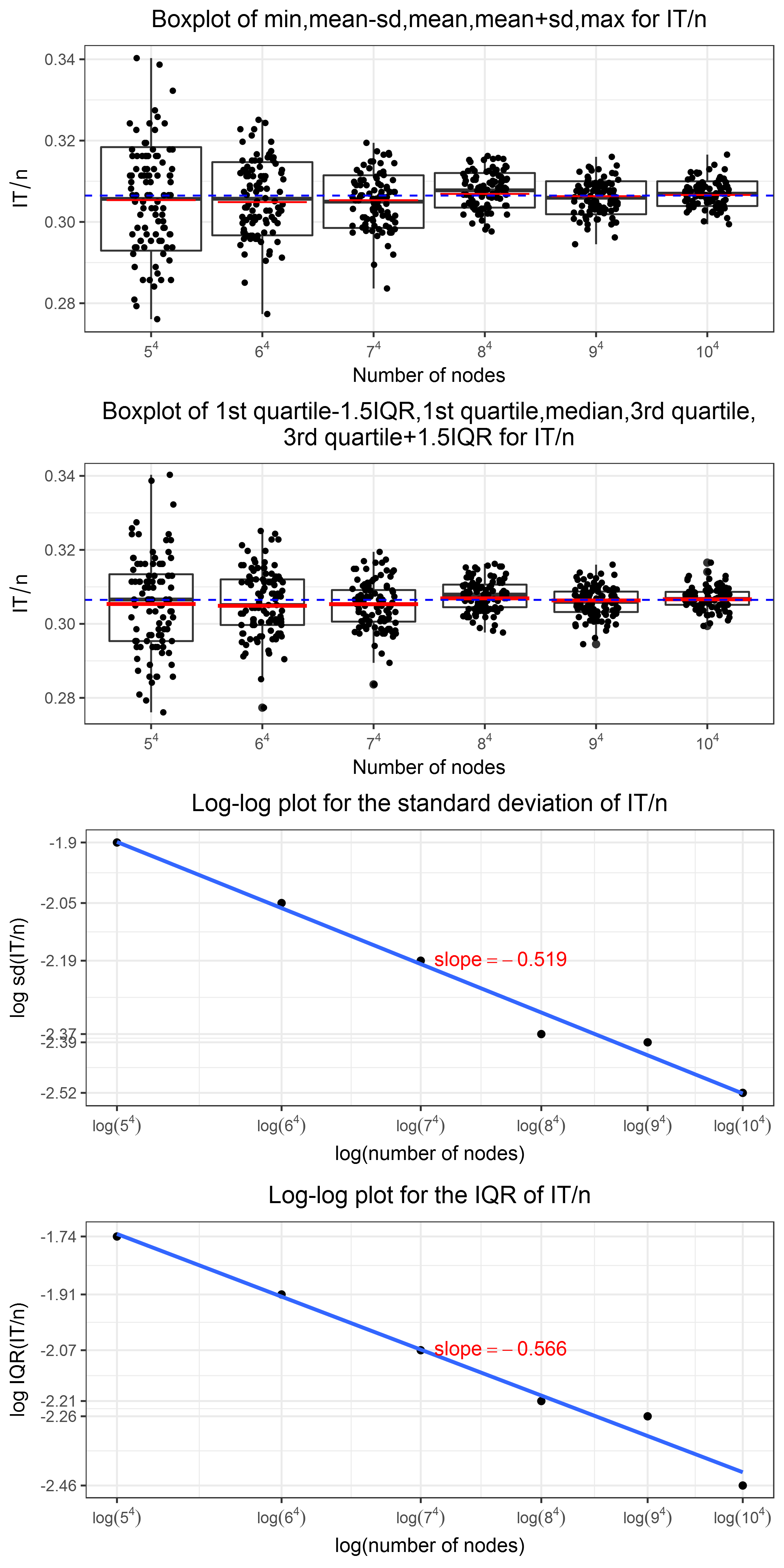
Figure 13.1. The boxplot and log-log plot of standard deviation and IQR for $IT/n$ under optimal policy

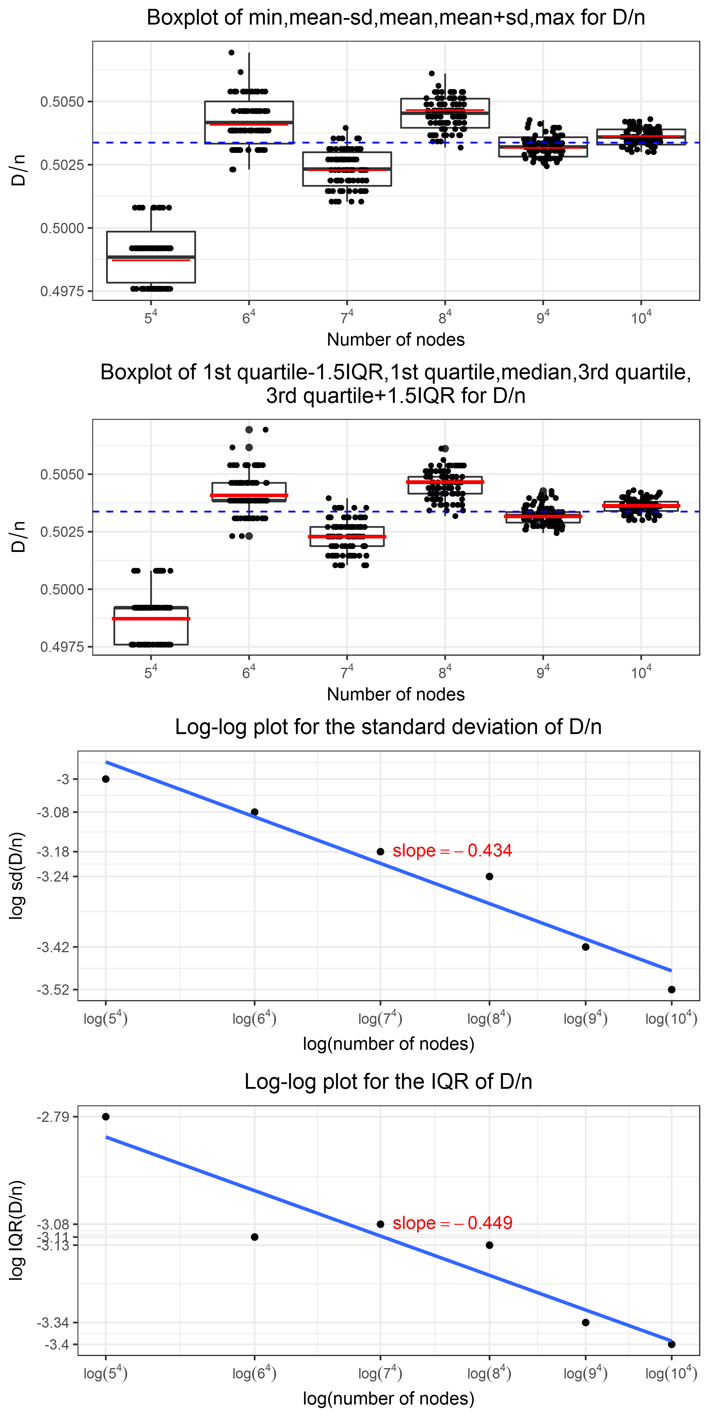
Figure 13.2. The boxplot and log-log plot of standard deviation and IQR for $D/n$ under optimal policy

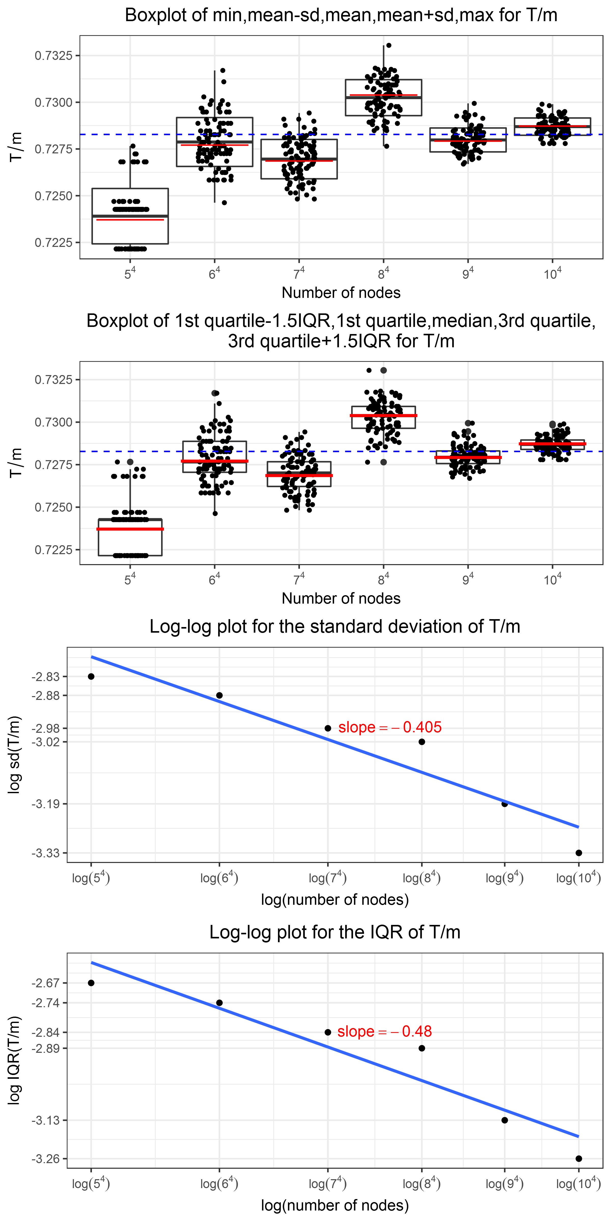
Figure 13.3. The boxplot and log-log plot of standard deviation and IQR for $T/m$ under optimal policy

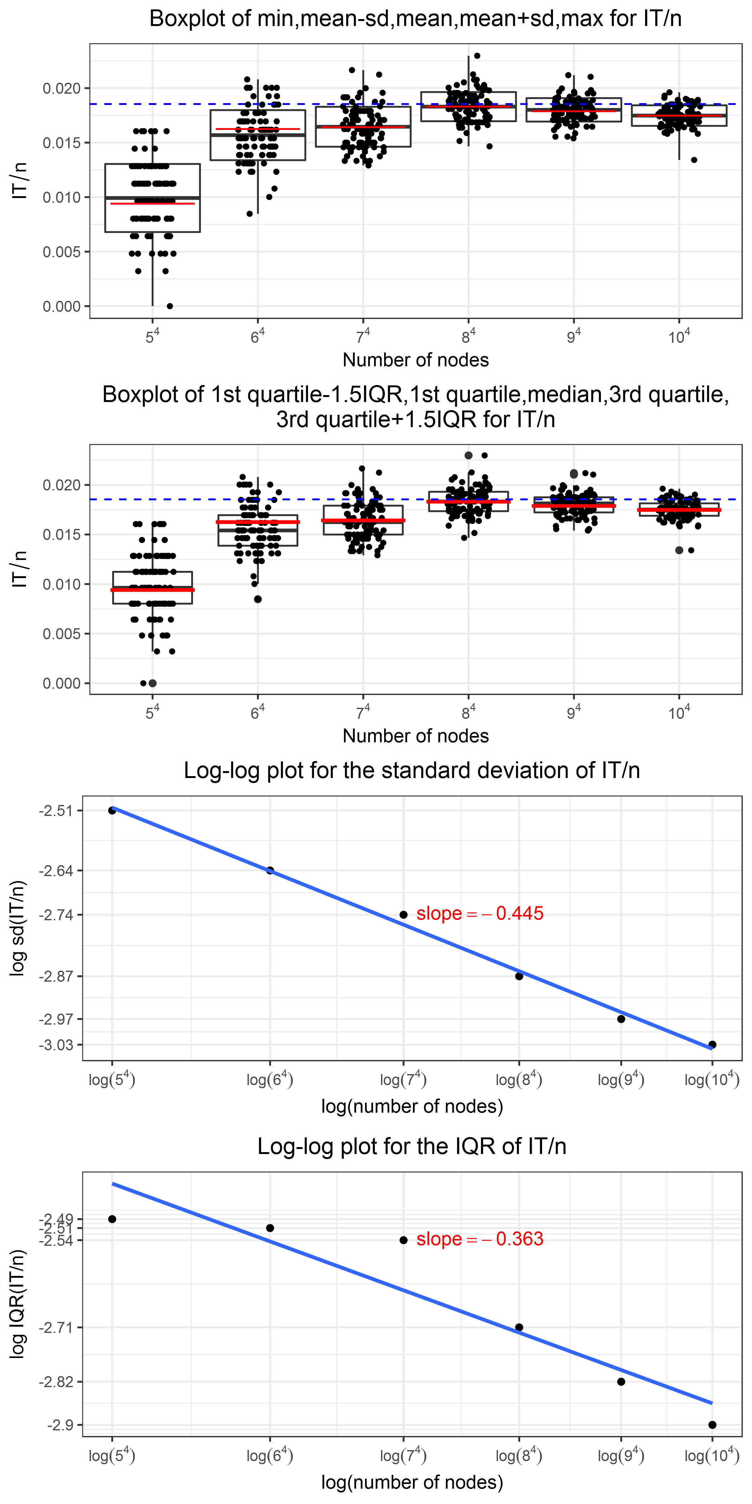
Figure 13.4. The boxplot and log-log plot of standard deviation and IQR for $IT/n$ under alternative policy

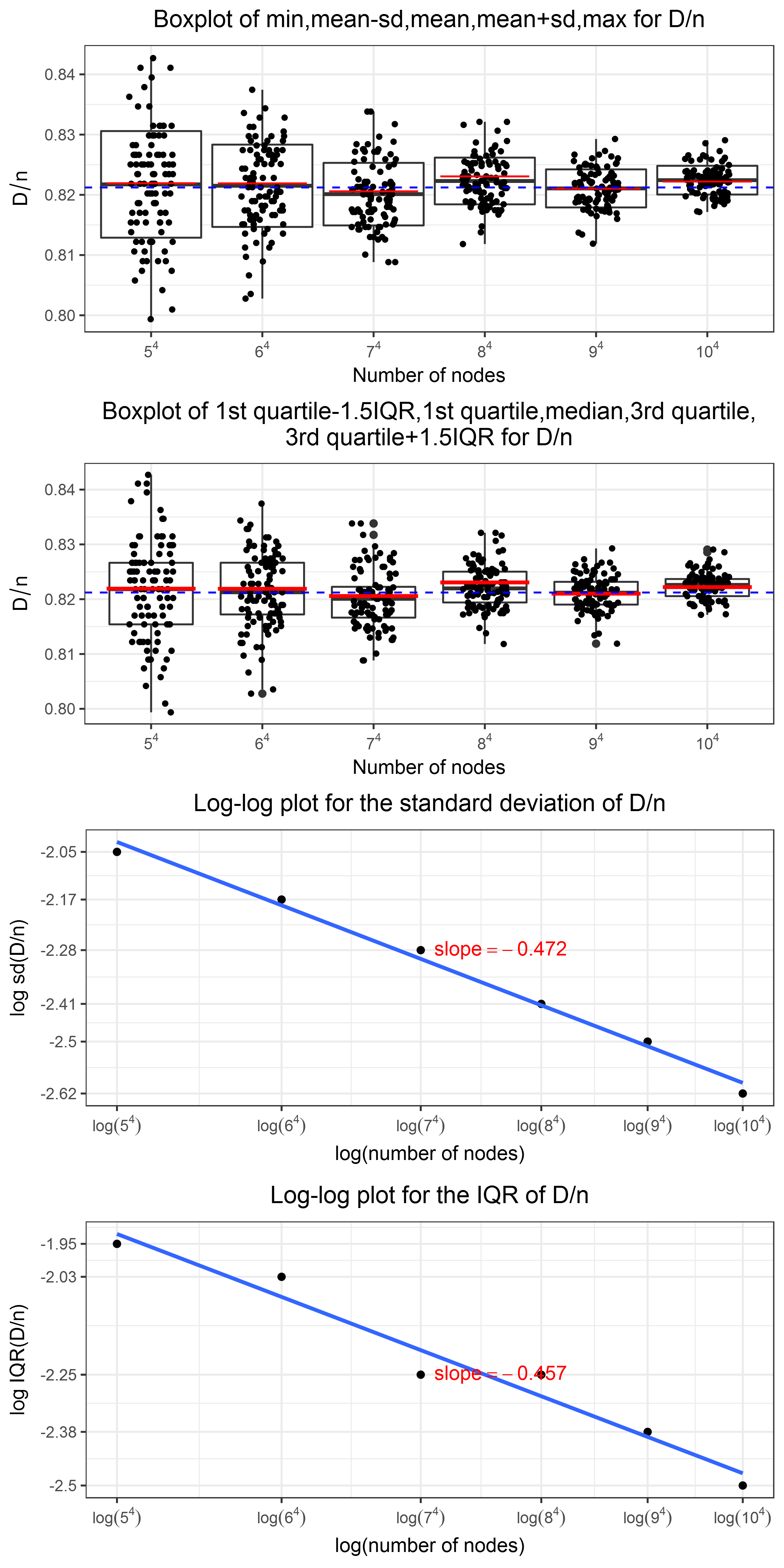
Figure 13.5. The boxplot and log-log plot of standard deviation and IQR for $D/n$ under alternative policy

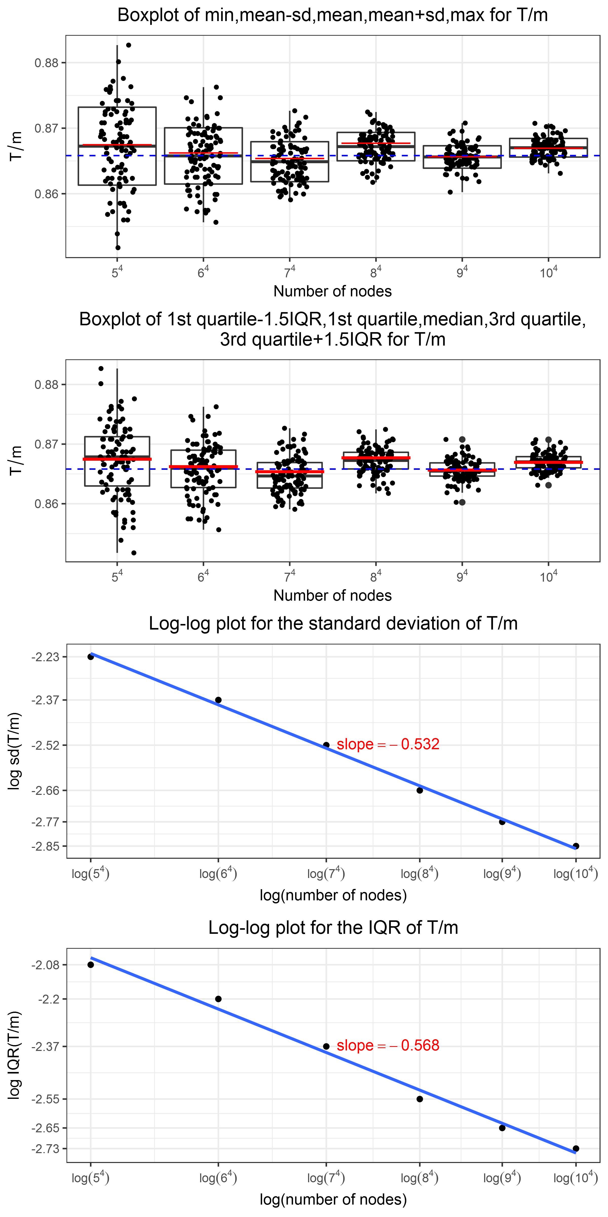
Figure 13.6. The boxplot and log-log plot of standard deviation and IQR for $T/m$ under alternative policy

Part V Summary

We model the default contagion process in a large heterogeneous financial network viewed by a regulator outside the network whose goal is to minimize the number of final defaulted nodes with the minimum amount of interventions. The regulator has only partial information in that the connections of the nodes are unknown in the beginning but revealed as the contagion process involves. The partial information setting aligns with the reality better than most of the existing literature.

Our work extend the previous literature, in particular Amini et al. (2013, 2015, 2017) in that we provide analytical asymptotic results of the optimal intervention policy for the regulator and the fraction of final defaulted nodes for a heterogeneous network with a given arbitrary degree sequence and arbitrary initial equity levels. Our results of the optimal intervention policies generates insights in the perspectives of both random network processes and regulations. The optimal intervention policy first depends on the intervention cost: the lower the cost is, the more interventions we implement. We only need to consider intervening on a bank if it has distance to default of one when affected, i.e. the bank is very close to default. Moreover, we observe that the optimal intervention policy is monotonic with respect to the characteristics of the network: the larger the out degree is, the smaller the in degree is, and the higher the sum of initial equity levels and number of interventions received, the earlier we should begin to intervene on the node. Moreover, we should keep intervening on a node once we have intervened on it. In other words, we do not allow a node that has received interventions to default. We also quantify the improvements made by the optimal intervention policy in terms of the features of the network. Our simulation results show a good alignment with the theoretical calculations. The numerical studies also provide evidence that although the optimal intervention policy and the fraction of final default nodes are in asymptotic sense, they provide good approximations for large but realistic size of networks.

Part VI Appendix

Appendix A Wormald’s theorem

Lemma A.1.

(Wormald [1999])Let $a\geq 2$ be a fixed integer and $\left(\left(Y_{t}^{l}\right)_{1\leq l\leq a}\right)_{t\geq 0}$ denote a sequence of real valued random variables indexed by $n$ with its natural filtration $(\mathcal{F}_{t})_{t\geq 0}$. Assume that there is a constant $C_{0}>0$ such that $\left|Y_{t}^{l}\right|\leq C_{0}n$ for $\forall\,n,\,t\geq 0$ and $1\leq l\leq a$. Let $f_{l}:\,\mathbb{R}^{a+1}\rightarrow\mathbb{R}$ be functions and $U\subseteq\mathbb{R}^{a+1}$ be some bounded connected open set containing the closure of

(A.0.1) $$\left\{(0,z^{1},\ldots,z^{a}):\,\mathbb{P}(Y_{0}^{l}=z^{l}n,\,1\leq l\leq a)\neq 0\text{ for some }n\right\}.$$

Define the stopping time $T_{U}=\inf\left\{t\geq 1:\>(\frac{t}{n},\frac{Y_{t}^{1}}{n},\ldots,\frac{Y_{t}^{a}}{n})\notin U\right\}$. Assume the following three conditions are satisfied:

1. (Boundedness) For some function $\rho_{1}=\rho_{1}(n)\geq 1$ and $\forall t<T_{U}$ and $1\leq l\leq a$,

   (A.0.2) $$|Y_{t+1}^{l}-Y_{t}^{l}|\leq\rho_{1}.$$

2. (Trend) For some function $\rho_{2}=\rho_{2}(n)=o(1)$ and $\forall t<T_{U}$ and $1\leq l\leq a$,

   (A.0.3) $$\left|\mathbb{E}\left(Y_{t+1}^{l}-Y_{t}^{l}\mid\mathcal{F}_{t}\right)-f_{l}(\frac{t}{n},\frac{Y_{t}^{1}}{n},\ldots,\frac{Y_{t}^{a}}{n})\right|\leq\rho_{2}.$$

3. (Lipschitz continuity) The functions $(f_{l})_{1\leq l\leq a}$ are continuous and satisfies a Lipschitz condition on

   (A.0.4) $$U\cap\{(t,z^{1},\ldots,z^{a}):t\geq 0\}$$

   with the same Lipschitz constant for each $l$.

Then the following holds:

1. For $(0,\hat{z}^{1},\ldots,\hat{z}^{a})\in U$ the system of differential equations

   (A.0.5) $$\frac{dz^{l}}{ds}=f_{l}(s,z^{1},\ldots,z^{a}),\qquad 1\leq l\leq a$$

   has a unique solution in $U$ for $z^{l}:\mathbb{R}\rightarrow\mathbb{R}$ passing through

   (A.0.6) $$z_{0}^{l}=\hat{z}^{l},\qquad 1\leq l\leq a$$

   and which extends to points arbitrarily close to the boundary of $U$.

2. Let $\rho>\rho_{2}$ and $\rho=o(1)$. For a sufficiently large constant C, with probability $1-O\left(\frac{\rho_{1}}{\rho}\exp\left(-\frac{n\rho^{3}}{\rho_{1}^{3}}\right)\right)$, it holds that

   (A.0.7) $$\sup_{0\leq t\leq n\sigma}\left(\frac{Y_{t}^{l}}{n}-z_{\frac{t}{n}}^{l}\right)=O(\rho)$$

   where $z_{s}^{l}$ is the solution in (1) with

   (A.0.8) $$z_{0}^{l}=\frac{Y_{0}^{l}}{n}$$

   and

   (A.0.9) $$\sigma=\sigma(n)=\sup\left\{s\geq 0:\,d_{\infty}\left(((z_{s}^{l})_{1\leq l\leq a}),\partial U\right)\geq C\rho\right\},$$

   where $d_{\infty}(u,v)=\max_{1\leq i\leq j}|u_{i}-v_{i}|$ for $u=(u_{1},\ldots,u_{j})\in\mathbb{R}^{j}$ and $v=(v_{1},\ldots,v_{j})\in\mathbb{R}^{j}$.

Appendix B Extended Pontryagin maximum principle

Lemma B.1.

(Extended Pontryagin maximum principle, Chachuat [2009]) Consider the optimal control problem to minimize the cost functional including a terminal term

(B.0.1) $$\mathcal{J}(u,t_{f})\coloneqq\int_{t_{0}}^{t_{f}}\ell(t,x_{t},u_{t})dt+\phi(t_{f},x_{t_{f}}),$$

with fixed initial time $t_{0}$ and free terminal time $t_{f}$, subject to the dynamical system

(B.0.2) $$\dot{x}_{t}=f(t,x_{t},u_{t});\quad x_{t_{0}}=x_{0},$$

where the vector function $x\in\hat{C^{1}}[t_{0},T]^{n_{x}}$ represents the state variables characterizing the behavior of the system at any time instant $t$, and some general terminal constraints

(B.0.3) $$\psi_{k}(t_{f},x_{t_{f}})=0,\quad k=1,\ldots,n_{\psi}.$$

The admissible controls shall be taken in the class of piecewise continuous functions

(B.0.4) $$u\in\mathcal{U}[t_{0},T]\coloneqq\{u\in\hat{C}[t_{0},T]^{n_{u}}:u_{t}\in U\text{ for }t_{0}\leq t\leq t_{f}\},$$

with $t_{f}\in[t_{0},T]$, where $T>t_{0}$ and the nonempty, possibly closed and nonconvex set $U$ denotes the control region.

Suppose $\ell$ and $f$ are continuous and have continuous first partial derivatives with respect to $(t,x,u)$ on $[t_{0},T]\times\mathbb{R}^{n_{x}}\times\mathbb{R}^{n_{u}}$, and also $\phi$ and $\psi\coloneqq(\psi_{k})_{k=1,\ldots,n_{\psi}}$ are continuous and have continuous first partial derivatives with respect to $(t,x)$ on $[t_{0},T]\times\mathbb{R}^{n_{x}}$. Suppose that the terminal constraints (B.0.3) satisfy the constraint qualification

(B.0.5) $$\text{rank}\left(\frac{\partial\psi}{\partial x}(t_{f}^{*},x_{t_{f}^{*}}^{*})\right)=n_{\psi}$$

where $\frac{\partial\psi}{\partial x}(t_{f}^{*},x_{t_{f}^{*}}^{*})$ denotes the Jacobian matrix of the partial derivatives of components of $\psi$ with respect to $x$ evaluated at $(t_{f}^{*},x_{t_{f}^{*}}^{*})$. Define the Hamiltonian function

(B.0.6) $$\mathcal{H}(t,x,u,\mathring{\lambda},\lambda)=\mathring{\lambda}\ell(t,x,u)+\lambda^{T}f(t,x,u).$$

Let $(u^{*},t_{f}^{*})\in\hat{C}[t_{0},T]^{n_{u}}\times[t_{0},T)$ denote a minimizer for the problem, and $x^{*}\in\hat{C^{1}}[t_{0},T]$ the optimal state, then there exists a $n_{x}$ dimensional piecewise continuously differentiable vector function $\lambda_{t}^{*}$ and $\mathring{\lambda}^{*}\in\{0,1\}$ ($(\mathring{\lambda}^{*},\lambda_{t}^{*})$ are called adjoint variables) and a Lagrange multiplier vector $v^{*}\in\mathbb{R}^{n_{\psi}}$ such that $(\mathring{\lambda}^{*},\lambda_{t}^{*})\neq 0$ for every $t\in[t_{0},t_{f}^{*}]$ and the following conditions hold:

1. The function $\mathcal{H}(t,x_{t}^{*},w,\mathring{\lambda}^{*},\lambda_{t}^{*})$ attains its minimum on $U$ at $w=u_{t}^{*}$ for every $t\in[t_{0},t_{f}^{*}]$, i.e.

   (B.0.7) $$\mathcal{H}(t,x_{t}^{*},w,\mathring{\lambda}^{*},\lambda_{t}^{*})\geq\mathcal{H}(t,x_{t}^{*},u_{t}^{*},\mathring{\lambda}^{*},\lambda_{t}^{*}),\quad\forall w\in U.$$

2. $(x_{t}^{*},u_{t}^{*},\mathring{\lambda}^{*},\lambda_{t}^{*})$ verifies the equations

   $$\frac{d}{dt}x_{t}^{*} =f(t,x_{t}^{*},u_{t}^{*})$$

   (B.0.8) $$\frac{d}{dt}\lambda_{t}^{*} =-\frac{\partial}{\partial x}\mathcal{H}(t,x_{t}^{*},u_{t}^{*},\mathring{\lambda}^{*},\lambda_{t}^{*})$$

   at each instant $t$ of continuity of $u^{*}$ and $\mathring{\lambda}^{*}\in\{0,1\}$.

3. $\mathcal{H}(t,x_{t}^{*},u_{t}^{*},\mathring{\lambda}^{*},\lambda_{t}^{*})=\mathcal{H}(t_{f}^{*},x_{t_{f}^{*}}^{*},u_{t_{f}^{*}}^{*},\mathring{\lambda}^{*},\lambda_{t_{f}^{*}}^{*})-\int_{t}^{t_{f}^{*}}\frac{\partial}{\partial t}\mathcal{H}(\tau,x_{\tau}^{*},u_{\tau}^{*},\mathring{\lambda},\lambda_{\tau}^{*})d\tau$. Therefore, if $\frac{\partial}{\partial t}\mathcal{H}=0$, i.e. $\mathcal{H}$ is autonomous, then $\mathcal{H}$ is a constant over time.

4. (Transversal condition) Define $\Psi(t,x)\coloneqq\mathring{\lambda}^{*}\phi(t,x)+v^{*T}\psi(t,x)$, then

   $$\lambda_{t_{f}^{*}}^{*} = \frac{\partial}{\partial x}\Psi(t_{f}^{*},x_{t_{f}^{*}}^{*})$$

   (B.0.9) $$\mathcal{H}(t_{f}^{*},x_{t_{f}^{*}}^{*},u_{t_{f}^{*}}^{*},\mathring{\lambda}_{t_{f}^{*}}^{*},\lambda_{t_{f}^{*}}^{*}) = -\frac{\partial}{\partial t}\Psi(t_{f}^{*},x_{t_{f}^{*}}^{*})$$

   together with the terminal condition (B.0.3) at $t=t_{f}^{*}$, i.e. $\psi_{k}(t_{f}^{*},x_{t_{f}^{*}}^{*})=0$ for $k=1,\ldots,n_{\psi}$.

5. The optimal control $u^{*}$ may or may not be continuous; in the latter case we have a corner point. In particular, the conditions that must hold at any corner point $\theta\in[t_{0},t_{f}^{*}]$ are

   $$x_{\theta^{-}}^{*} = x_{\theta^{+}}^{*},$$

   $$\lambda_{\theta^{-}}^{*} = \lambda_{\theta^{+}}^{*},$$

   (B.0.10) $$\mathcal{H}(\theta^{-},x_{\theta}^{*},u_{\theta^{-}}^{*},\mathring{\lambda}^{*},\lambda_{\theta}^{*}) = \mathcal{H}(\theta^{+},x_{\theta}^{*},u_{\theta^{+}}^{*},\mathring{\lambda}^{*},\lambda_{\theta}^{*}).$$

Proof.

See theorem 3.33 and theorem 3.34 in Chachuat [2009]. ∎

References

- Amini et al. [2013] Hamed Amini, Rama Cont, and Andreea Minca. Resilience to contagion in financial networks. Mathematical Finance, 00(0):1–37, 2013.
- Amini et al. [2015] Hamed Amini, Andreea Minca, Hamed Amini, and Andreea Minca. Control of interbank contagion under partial information. Journal of Financial Mathematics, 6(1):24, 2015.
- Amini et al. [2017] Hamed Amini, Andreea Minca, and Agnès Sulem. Optimal equity infusions in interbank networks. Journal of Financial Stability, 31:1–17, 2017. ISSN 1572-3089.
- Cont et al. [2010a] Rama Cont, Amal Moussa, and Edson Bastos e Santos. Network Structure and Systemic Risk in Banking Systems. SSRN Electronic Journal, pages 327–368, 2010a. ISSN 1556-5068. doi: 10.2139/ssrn.1733528. URL http://ssrn.com/paper=1733528 http://www.ssrn.com/abstract=1733528.
- Furfine [2003] Craig H Furfine. Interbank Exposures: Quantifying the Risk of Contagion. Journal of Money, Credit and Banking, 35(1):pp. 111–128, 2003. ISSN 00222879. doi: 10.2307/3649847. URL http://www.jstor.org/stable/3649847.
- Cont et al. [2010b] Rama Cont, Amal Moussa, and Edson B. Santos. Network Structure and Systemic Risk in Banking Systems. SSRN eLibrary, 2010b. ISSN 15565068. doi: 10.2139/ssrn.1733528. URL http://ssrn.com/paper=1733528.
- Boss and Elsinger [2004] Michael Boss and Helmut Elsinger. An empirical analysis of the network structure of the Austrian interbank market. Financial stability Report, pages 77–87, 2004.
- Allen and Gale [2000] Franklin Allen and Douglas Gale. Financial contagion. Journal of Political Economy, 1(108):1–33, 2000.
- May and Arinaminpathy [2010] Robert M May and Nimalan Arinaminpathy. Systemic risk: the dynamics of model banking systems. Journal of the Royal Society, Interface / the Royal Society, 7:823–838, 2010. ISSN 1742-5689.
- Haldane and May [2011] Andrew G Haldane and Robert M May. Systemic risk in banking ecosystems. Nature, 469:351–355, 2011. ISSN 0028-0836. doi: 10.1038/nature09659.
- Gai et al. [2011] Prasanna Gai, Andrew Haldane, and Sujit Kapadia. Complexity, concentration and contagion. Journal of Monetary Economics, 58:453–470, 2011. ISSN 03043932. doi: 10.1016/j.jmoneco.2011.05.005.
- Nier et al. [2007] Erlend Nier, Jing Yang, Tanju Yorulmazer, and Amadeo Alentorn. Network models and financial stability, 2007. ISSN 01651889.
- Eisenberg and Noe [2001] Larry Eisenberg and Thomas H. Noe. Systemic Risk in Financial Systems, 2001. ISSN 0025-1909.
- Hurd [2015] T. R. Hurd. Contagion! The Spread of Systemic Risk in Financial Networks. 2015.
- Song and van der Schaar [2015] Yangbo Song and Mihaela van der Schaar. Dynamic network formation with incomplete information. Economic Theory, jan 2015. ISSN 0938-2259. doi: 10.1007/s00199-015-0858-y. URL http://link.springer.com/10.1007/s00199-015-0858-y.
- Battiston et al. [2012] Stefano Battiston, Domenico Delli Gatti, Mauro Gallegati, Bruce Greenwald, and Joseph E. Stiglitz. Default cascades: When does risk diversification increase stability? Journal of Financial Stability, 8:138–149, 2012. ISSN 15723089. doi: 10.1016/j.jfs.2012.01.002.
- van der Hofstad [2014] Remco van der Hofstad. Random Graphs and Complex Networks. 2014.
- Furfine [1999] Craig H. Furfine. The Microstructure of the Federal Funds Market. Financial Markets, Institutions and Instruments, 8(5):24–44, 1999. ISSN 0963-8008.
- Bech and Atalay [2010] Morten L. Bech and Enghin Atalay. The topology of the federal funds market. Physica A: Statistical Mechanics and its Applications, 389(22):5223–5246, 2010. ISSN 03784371.
- Wormald [1999] N.C. Wormald. The Differential Equation Method for Random Network Processes and Greedy Algorithms. In Lectures on Approximation and Randomized Algorithms, pages 73–155. 1999.
- Chachuat [2009] Benoit C. Chachuat. Nonlinear and Dynamic Optimization: From Theory to Practice - IC-32: Spring Term 2009. EPFL, 2009.