From the arrow of time in Badiali’s quantum approach to the dynamic meaning of Riemann’s hypothesis

Abstract

The novelty of the Jean Pierre Badiali last scientific works stems to a quantum approach based on both (i) a return to the notion of trajectories (Feynman paths) and (ii) an irreversibility of the quantum transitions. These iconoclastic choices find again the Hilbertian and the von Neumann algebraic point of view by dealing statistics over loops. This approach confers an external thermodynamic origin to the notion of a quantum unit of time (Rovelli Connes’ thermal time). This notion, basis for quantization, appears herein as a mere criterion of parting between the quantum regime and the thermodynamic regime. The purpose of this note is to unfold the content of the last five years of scientific exchanges aiming to link in a coherent scheme the Jean Pierre’s choices and works, and the works of the authors of this note based on hyperbolic geodesics and the associated role of Riemann zeta functions. While these options do not unveil any contradictions, nevertheless they give birth to an intrinsic arrow of time different from the thermal time. The question of the physical meaning of Riemann hypothesis as the basis of quantum mechanics, which was at the heart of our last exchanges, is the backbone of this note.

Key words: path integrals, fractional differential equation, zeta functions, arrow of time

PACS: 05.30.-d, 05.45.-a, 11.30.-j, 03.65.Vf

Abstract

Íîâèçíà îñòàííiõ íàóêîâèõ ðîáiò Æàíà-Ï’єðà Áàäiàëi áåðå ïîчàòîê ç êâàíòîâîãî ïiäõîäó, ÿêèé áàçóєòüñÿ íà (i) ïîâåðíåííi äî ïîíÿòòÿ òðàєêòîðié (òðàєêòîði¿ Ôåéíìàíà), à òàêîæ íà (ii) íåîáîðîòíîñòi êâàíòîâèõ ïåðåõîäiâ. Öi iêîíîêëàñòèчíi âàðiàíòè çíîâó âñòàíîâëþþòü ãiëüáåðòiàí i àëãåáðà¿чíó òîчêó çîðó ôîí Íåéìàíà, ìàþчè ñïðàâó çi ñòàòèñòèêîþ çà öèêëàìè. Öåé ïiäõiä íàäàє çîâíiøíþ òåðìîäèíàìiчíó ïåðøîïðèчèíó ïîíÿòòþ êâàíòîâî¿ îäèíèöi чàñó (òåðìàëüíèé чàñ Ðîâåëëi Êîííåñà). Öå ïîíÿòòÿ, áàçèñ äëÿ êâàíòóâàííÿ, âèíèêàє òóò ÿê ïðîñòèé êðèòåðié ðîçðiçíåííÿ ìiæ êâàíòîâèì ðåæèìîì i òåðìîäèíàìiчíèì ðåæèìîì. Ìåòà öiє¿ ñòàòòi є ðîçêðèòè çìiñò îñòàííiõ ï’ÿòè ðîêiâ íàóêîâèõ äèñêóñié, íàöiëåíèõ ç’єäíàòè â êîãåðåíòíó ñõåìó ÿê óïîäîáàííÿ i ðîáîòè Æàíà-Ï’єðà, òàê i ðîáîòè àâòîðiâ öiє¿ ñòàòòi íà îñíîâi ãiïåðáîëiчíî¿ ãåîäåçi¿, i îá’єäíóþчó ðîëü äçåòà-ôóíêöi¿ Ðiìàíà. Õîчà öi âàðiàíòè íå ïðåäñòàâëÿþòü æîäíèõ ïðîòèðiч, òèì íå ìåíøå, âîíè ïîðîäæóþòü âëàñíó ñòðiëó чàñó, iíàêøó íiæ òåðìàëüíèé чàñ. Ïèòàííÿ ôiçèчíîãî çìiñòó ãiïîòåçè Ðiìàíà ÿê îñíîâè êâàíòîâî¿ ìåõàíiêè, ùî áóëî â öåíòði íàøèõ îñòàííiõ äèñêóñié, є ñóòòþ öiє¿ ñòàòòi.

Ключовi слова: iíòåãðàëè çà òðàєêòîðiÿìè, äèôåðåíöiàëüíi ðiâíÿííÿ â чàñòêîâèõ ïîõiäíèõ, äçåòà-ôóíêöi¿, ñòðiëà чàñó

1 From algebraic analysis of quantum mechanics to “irreversible” Feynman paths integral

Despite the unstoppable success of the technosciences based on both quantum mechanics, standard particle model and cosmological model, at least two questions must be investigated among many issues that the theories leave open [1, 2]: (i) the question of the ontological status of the time and (ii) the obsessive interrogation concerning the existence or the absence of an intrinsic “arrow of time”. The origin of these questions comes from the equivocal equivalence of the status of time in any types of mechanical formalisms. For example, within Newtonian vision, the observable $f$ can be analysed algebraically using action-integral through the Lagrangian $L$ while Poisson brackets gives time differential representations $\mathrm{d}f/\mathrm{d}t=\{H,f\}$. According to Noether theorem, the energy, referred to the Hamiltonian $H$, is no other than the tag of a time-shift independence of physical laws, namely a compact commutativity. The statistical knowledge of the high dimensions system requires (i) the definition of a Liouville measure $\mu_{\text{L}}$ based on the symplectic structure of the phase space and (ii) the value of the configuration distribution $Z_{\text{C}}$, therefore $\mathrm{d}\mu\sim(1/Z_{\text{C}})\,\mathrm{e}^{-\beta H}$, with $\beta=1/k_{\text{B}}T$ related to the inverse of the temperature. This point of view is discretized in quantum mechanics (QM).

With regard to quantum perspectives, mechanical formalism introduces (i) a thickening of the mechanical dot, (ii) the substitution of real variables through the spectrum of operators and (iii) an emphasis on the role of probability. According to von Neumann, the stable core of the operator algebra required to fit the quantum data must be based upon groupoids acting on observables. In the Heisenberg framework, the observable $\hat{f}$ (for instance the paradigmatic example of the set of the rays of materials emissions) is represented by self-adjoint operators in Hilbert space $l^{2}(\mathbb{R}^{3},\mathbb{C}$) which values can be reduced within Born-matrix representation to a set of eigenvectors $|\varphi_{n}\rangle$ chosen in the spectrum $\operatorname{spec}(\hat{f})$ of the groupoid. Energy distribution is given through the linear relations $\hat{H}|\varphi_{n}\rangle=E|\varphi_{n}\rangle$, where the Hamiltonian $\hat{H}$ represents the energy self-adjoint operator. The dynamics is implemented by using the commutator: $[\hat{H},\hat{f}]$ which replaces the Poisson bracket, namely $\mathrm{d}\hat{f}(t)/\mathrm{d}t=\frac{2\piup\mathrm{i}}{h}[\hat{H},\hat{f}]$. The capability of giving cyclic representations of von Neumann algebra (extended to Weyl non-commutative algebra for standard model) leads to expressing the dynamics via the eigenvectors Fourier components $|\psi_{n}(t)\rangle=|\varphi_{n}\rangle\exp(-\mathrm{i}E_{n}t/\hbar)$. This representation is unitarily equivalent to a wave mechanics usually expressed through the Schrödinger equation, $\mathrm{i}\hbar\frac{\mathrm{d}}{\mathrm{d}t}\psi(r,t)=[-\frac{\hbar^{2}}{2m}\nabla^{2}+V(r,t)]\psi(r,t)$. The shift from non-linear finite to linear infinite system must be based upon the statistics dealing with a $\Lambda$-extension of the system, through a linear and positive forms $\hat{f}\in A$ $\Phi_{\Lambda}(A)=(1/Z_{\text{C}})\operatorname{Tr}\exp(-\beta H_{\Lambda_{A}})$. Hence, the average value of the observable $\hat{f}\in A$ is a trace of an exponential operator. Usually, the distribution of physical data must be given by a measure of probability on $\operatorname{spec}(A)$. Thus, we cannot deal with QM without dealing with Gaussian randomness imposed by some external thermostat. At this step, a useful notion is the notion of density matrix given by: $\rho N=\exp(-\beta H)$. Unfortunately, $N$ the normalization constant suffers from all misgivings involved in thermodynamics, by the “shaky” notion of equilibrium.

Each item of the above visions imposes its own algebraic constraints but enforces a paradigmatic concept of time parameter [3] as a reversible ingredient of the physics. At this step, the statistics appears as the only loophole capable of introducing irreversibility as a path to an assumptive equilibrium state for finite $\beta$ value. Nevertheless, as shown above, this assumption requires the $\Lambda$-extension, namely, the transfer of the operator algebra in the framework of C*-algebra in which the $A$-algebra of its Hermitian elements patterns the transfer (rays) between a set of perfectly well defined states. Starting from the notion of groupoid and from the algebra of magma upon the states and by analysing the symmetries, a mathematician can also consider the equilibrium from a set of cyclic states $\Omega$ of $\hat{f}$, based on Gelfand, Naimark, Segal construction (GNS construction) [5] binding quantum states and the cyclic states (cyclic transfer which assumes a specific role of scalar operators, called $M$-factors). At this stage, two points of view must be matched together to make the irreversibility emerge from $M$: (i) Tomita Takesaki’s dynamic theory [6] extended by Connes [3, 4] and (ii) Kubo, Martin and Schwinger KMS physical principle [7].

• According to Tomita-Takesaki, if $A$ is a von Neumann algebra, there exists a modular automorphism group $\Delta$ based on a sole parameter $t$: $\alpha_{t}=\Delta^{-\mathrm{i}t}A\Delta^{+\mathrm{i}t}$ which leaves the algebra invariant: $\mathrm{d}\alpha_{t}(A)/\mathrm{d}t=\lim_{\Lambda\rightarrow\infty}(2\piup\mathrm{i}/h)[H_{\Lambda}A]$. There is a canonical homomorphism from the additive group of reals to the outer automorphism group of $A$: $B$, that is independent of the choice of “faithful” state. Therefore, $\langle\Omega,B(\alpha_{t+j}A)\Omega\rangle=\langle\Omega,(\alpha_{t}A)B\Omega\rangle$, where $(\,,)$ is the inner product.

• The link with KMS physical constraint extends this abstract point of view. The dynamics expression using the Kubo density matrix allows one to change the “shaky” hypothesis of thermodynamic equilibrium by giving it a dynamical expression. KMS suggested to define the equilibrium from a correlation function $[(\gamma_{t}A)B]=[B(\gamma_{t+\mathrm{i}\beta h}A)]$ allowing to associate the equilibrium with a Hamiltonian according to $\gamma_{t}A=\exp(\mathrm{i}tH/h).A.\exp(-\mathrm{i}tH/h)$.

The matching of both sections leads: $\beta h=1$ which is nothing but the emergence of a thermodynamic gauge of time while the time variable stays perfectly reversible [3].

Starting from this analysis Jean Pierre Badiali (JPB) decided the exploration of QM by using the local irreversible transfer joined to Feynman [8] path integrals model based on an iconoclast existence of 2D self-similar “trajectories”. While this model suffers from mathematical divergences and requires questionable renormalisation operations, Feynman model efficiency was rapidly attested. Nevertheless, many physicists still considered that Feynman integrals are meaningless because the concept of trajectory should “obviously” not be relevant in QM. The discernment of JPB was to take the same trail as Feynman, by imagining irreversible series of transition giving birth to real self-similar paths at particles. By using a Feynman Kac transfer formula for conditional expectation of transfer, he writes $q(x_{0},t_{0},x,t)=\int Dx(t)\exp[-\frac{1}{\hbar}A(x_{0},t_{0};x,t)]$ in which the rules of transfer are based on a Newtonian action $A(x_{0},t_{0};x,t)=\intop\{\frac{1}{2}m[\frac{\mathrm{d}x(s)}{\mathrm{d}s}]^{2}+u[x(s)]\}\mathrm{d}s$, he wrote the solution required for discretizing the trajectories [9]. These notions are not associated with any natural Hamiltonian and require a coarse graining of the space-time. To overcome this constraint, JPB considered the couple of functional probabilities $\phi(x,t)=\int\mathrm{d}y\phi_{0}(y)q(y,t_{0};x,t)$ and $\hat{\phi}(xt)=\int q(t,x;t_{1},y)\phi_{1}(y)\mathrm{d}y$ with $t_{1}>t>t_{0}$. The evolution of a system is given by a Laplacian propagator in which $\phi(x,t)$ is bended out by geometrical potential $u(x,t)$ according to $\pm\frac{\partial}{\partial t}\phi(x,t)+D\Delta\phi(x,t)=\frac{1}{\hbar}u(x,t)\phi(x,t)$, where $D=\hbar/2m$ is the quantic expression of a diffusion constant and $\phi(x,t)$ cannot be normed. These equations are neither Chapman-Kolmogorov equations nor Schrödinger like equations. Thenceforth, which physical and geometrical meaning may we attribute to the discreet arithmetic site on which the fractal-paths are based? How do the morphisms between states and trajectories determine the dynamical topos? How the statistical or non-statistical regularizations ruling the dynamics may smooth the experimental behavior? All these issues are open. To solve them, JPB point of view required a new visitation of the thermodynamics and in conformity with KMS point of view, a new definition of the equilibrium expressed via the irreversibility of the local transfer. To do this, he considered the class of the paths reduced to loops: $\phi(x_{0},t_{0},x_{0},t-t_{0})$ and their fluctuations in energy. Assuming an average energy $U$ determined by a thermostat, the overall fluctuations are ruled by a deviation, on the one hand, from the reference value $U$ and, on the other hand, from the number of loops concerned. As Feynman had imagined it, an entropy function: $S_{\text{path}}=k_{\text{B}}\ln\int q(x_{0}t_{0},x_{0},t-t_{0})\mathrm{d}x_{0}$ can be built which is ruled by the concept of path temperature $T_{\text{path}}$: $\frac{\hbar}{k_{\text{B}}}(1/T_{\text{path}})=\tau+[U-(\langle u_{K}\rangle_{\text{path}}+\langle u_{p}\rangle_{\text{path}})]\frac{\partial\tau}{\partial u}$. The emergence of an equilibrium is figured dynamically through a critical time scale $1/\beta h$, which possesses a strictly quantum statistical origin merely based on loops $\tau=(\hbar/k_{\text{B}})T_{\text{path}}$ if it can be assumed that the temperature of the integral of the path is none other than the usual thermodynamic temperature. From this step, JPB finds again the Rovelli-Connes assertions regarding thermal-time [10] and he proves the Boltzmann $H$-theorem. By means of subtle analysis using the duality of the couple propagators (forward and backward dynamics), he built a complex function $\psi,$ solution of the Schrödinger equation. The thought of JPB appears as a subtle adventure which — inscribed in the footsteps of Richard Feynman, and implemented from a deep knowledge of QM, thermodynamics, thermochemistry and irreversible processes — changes the traditional point of view and builds a perspective that we have to analyze now, from an alternative point of view which replaces the transport along the fractal trail by a transfer across an interface, both perspectives being strongly related. In brief, $1/\beta$ provides a scale of energy which smooths the regime of quantum fluctuations according to an uncertainty relation: $\Delta E=\hbar/\Delta t<1/\beta$ namely $\Delta t>\beta\hbar$. $\beta\hbar$ is the value of the time defining the cut-off between quantum fluctuations and thermodynamic fluctuations. The propagation function imparts a quadratic form to the spatial fluctuations, namely $\delta x^{2}=(\beta\hbar/\partial t-1)\partial t^{2}/m$. If $\Delta t=\beta\hbar/2$ then $\delta x^{2}=\beta\hbar^{2}/m=2\beta\hbar D\sim\delta t$, the value that, with the reserve of taking into account the entropy constant $k_{\text{B}}$, must be compared to de Broglie’s length. Thus, the coarse graining of the time will be considered as the dual of the quadratic quantification of space, when a length in this space can be reduced to the constraints imposed by the geometrical pattern of non-derivable trajectories (herein with a dimension two attributed implicitly and for quantum physical reasons to the set of Feynman paths). The aim of this note is to show that this “cognitive skeleton” does not only give birth to thermal statistical time, but through a generalization of fractal dimension, to a purely geometric irreversible time unit: an arrow of time.

2 Zeta function and “$\alpha$-exponantiation”

In addition to B. Mandelbrot initial friendship, we owe to J.P. Badiali and Professors I. Epelboin and P.G. de Gennes the first academic support for the development of the industrial TEISI model energy transfer on self-similar (i.e., fractal interfaces). This was at the end of seventies shortly before the premature death of Professor Epelboin. The purpose of this model was to explain the electrodynamic behavior of the lithium-ion batteries which were then at the stage of their first industrial predevelopment [11, 12, 13]. The interpretation and the patterning of electronic and ionic transfer coupled together in 2D layered positive materials $(\text{TiS}_{2},\text{NiPS}_{3})$ are very similar to the JPB model. The electrode is characterized by a fractal dimension $d$ which, due to the symmetries of real space, must be such as $d\in[1,2]$. When the fractal structure of the electrode is scanned by the transfer dynamics through electrochemical exchanges, the electrode does not behave like an Euclidean interface, as a straightforward separation between two media, but like an infinite set of sheets of approximations normed by $\eta(\omega)$ or a multi-sheet manifold, thick set of self-similar interfaces working as paralleled interfaces [14], where $\omega$ is a Fourier variable. Each $\eta(\omega)$-interface is tuned by a Fourier component of the electrochemical dynamics. The overall exchange is ruled by a transfer of energy either supplied by a battery (discharge) or stored inside the device (charge). The impedance of positive electrode is expressed through convolution operators coupled with the distributions of the sites of exchanges (electrode), giving birth at macroscopic level to a class of non-integer differential operators which take into account the laws of scaling, from quantum scales of transfer up to the macroscopic scales of measurement. This convolution between the discreet structure of the geometry and the dynamics must be written in Fourier space by using an extension of the Mandelbrot like fractal measure namely $N\eta^{d}=1$, into operator-algebra with $N=\mathrm{i}\omega\tau$ [11]. Mainly, the model emphasizes the concept of fractal capacity (fractance) — implicitly Choquet non-additive measure and integrals — whose charge is ruled by the non-integer differential equation $\mathrm{i}\sim\mathrm{d}^{\alpha}U/\mathrm{d}t^{\alpha}$ with $\alpha=1/d$ [15, 16], where $U$ is the experimental potential. In the simplest case of the first order local transfer, hence, for canonical transfer, the Fourier transform must be expressed through Cole and Cole type of impedance: $Z_{\alpha}(\omega)\sim 1/[1+(\mathrm{i}\omega\tau)^{\alpha}]$ [17, 18, 19, 20] which is a generalization of the exponential transfer turned by convolving with the $d$-fractal geometry. Many other interesting expressions and forms can be found, but being basically related to exponential operator, the canonic form appears as seminal. The model was confirmed experimentally in the frame of many convergent experiments concerning numerous types of batteries and dielectric devices. JPB has advised all these developments especially within controversies and intellectual showdowns. For instance, even if energy storage is at the heart of all engineering purposes [12, 13], the use of non-integer operators renders the model accountable of the fact that energy is no longer a natural Noetherian invariant of the new renormalizable representation. Therefore, algebraic and topological extensions must be considered whose results are the emergence of time-dissymmetry and of entropic-effects. Fortunately, $Z_{\alpha}(\omega)$ clearly appears as a geodesic of a hyperbolic space $\eta^{d}(\omega)=\frac{u}{v}$ authorizing (figure 1), on the one hand, the use of non-Euclidean metrics to establish a distance between $\eta(\omega)$-interfacial sheets and, on the other hand, the tricky algebraic and topological extension of the dynamics, practically a dual fractional expression of the exponential.

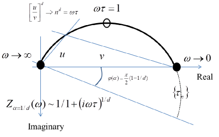
Figure 1: (Color online) Main characteristics of exponential transfer function convoluted by $d$-fractal geometry $1<d\leqslant 2$. If $d$ is the rightful non integer dimension of underlined geometry (TEISI model [11, 14]) the transfer function $Z_{\alpha}(\omega)$, — named Cole and Cole impedance in electrodynamics [11, 17, 18, 19], — finds its expression in $1/d$-exponantial (with “a”), a kind of degenerated time function in real space shaped by a hyperbolic geodesic close to an exponential in Fourier space. $Z_{\alpha}(\omega)$ is a hyperbolic geodesic in Fourier space. Reduced to its discrete representation in $\mathbb{N}$ or $\mathbb{\mathbb{Q}}$ such as $n=u/v$ or $v/u$ rational, $Z_{\alpha}^{N}(n)$ appears as the basis for the definition of $\zeta(s)$ Riemann function ($s=\alpha+\mathit{\mathrm{i}t}$) if $\mathit{\mathrm{i}t}$ expresses a mathematical fibration (figure 2). The singular points $\{0,1,\infty\}$ suggest links between $1/d$-exponantial and Teichmuller-Grothendick absolute Galois group. Adjoined with its categorical Kan extension $\tau$: $\{\tau_{n}\}$ obtained through the prime-decomposition $n=\omega\tau_{n}\in\mathbb{N}$ and playing the role of inverse Fourier transform, the above representation shapes, — via the pair of geodesics building the semi-circle, — the functional relationship between $\zeta(s)$ and $\zeta(1-\bar{s})$ [21, 23, 22].

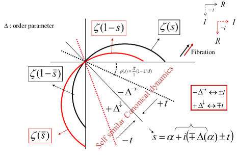
Figure 2: (Color online) Dynamical meaning of Riemann’s hypothesis, phases and arrow of time: Riemann zeta function $\zeta(s)$ is proved to be erected from a mathematical fibration $\pm\mathrm{i}t$ based on an $\alpha$-exponantiel represented in the oriented complex plan from $Z_{\alpha}^{N}(\omega)\cup\{\tau_{n}\}$ impedance (figure 1: direct in black and inverse in grey) when $\mathbb{N}$ quantization is carried out with $s=\alpha+\mathrm{i}t$. If $\alpha\neq 1/2$, the constraint of phase $\pm\Delta\neq 0$ over the fibration (gauge effect) is associated to the entropic properties of the dynamics while the phase involves a dissymmetry of the fibration parameter $\pm\mathrm{i}t$, therefore, $\zeta(s)\neq\zeta(\bar{s})$. If Riemann hypothesis is validated, $\alpha=1/2$ value associated to the quadratic self-similarity of the set of integers $\mathbb{N}\times\mathbb{N=\mathbb{N}}$, underlined Peano geometry. This hypothesis involves $\Delta=0$ and then $\zeta(s)=\zeta(\bar{s})$. With respect to $\alpha$-exponantiel, these properties can be expressed within a pair of vector bases: either based on phase angle $\varphi(\alpha)=\frac{\piup}{2}(1-\alpha)$ (determinism basis) or based on $\Delta(\alpha)$ (stochastic basis). The change from one to the other reference must be associated to a rotation of the dynamic referential keeping all non-linear properties $\alpha\neq 1/2$ of $\alpha$-geodesics. The $\Delta(\alpha)$ referential is, nevertheless, the most fundamental of both for at least two reasons: (i) The non-commutativity of successive $\theta$-rotations (groups) in the complex plan of $\zeta(s)$ definition can be expressed via the equation $\theta_{1}\circ\theta_{2}=\theta_{2}\circ\theta_{1}\mathrm{e}^{\pm 2\mathrm{i}\Delta}$, therefore, $\Delta(\alpha)=0$ implicitly provides a gauge condition for finding again the commutativity. Due to the phase effect, the symmetry $\zeta(s)=\zeta(1-\bar{s})$, the relation which naturally leads to $\zeta(s)=0$ as well as to the existence of Hilbert quantum mechanics states, matching here the random distribution of primes numbers (Montgomery hypothesis) according to the von Neumann algebra and multiplicative self-similarity of $\mathbb{N}$: $\mathbb{N}\times\mathbb{N=\mathbb{N}}$. The only solution to by-pass the resurgent symmetry of $t$ and to create dissymmetry is then to introduce statistics from outside via an external artefact: the thermostat ($t$ stays symmetric but the random fluctuations of local process rebuild the quantum time arrow through a so-called “thermal time” [9, 10, 27, 28]); (ii) The situation is opposite if the phase moves from zeros $\Delta(\alpha)\neq 0$. The loss of symmetry within the fibration keeps the internal non-commutativity leading to an intrinsic irreversibility of the time which may be named “arrow of time” [2]. Herein, this arrow finds its origin in the open status of the geometry highlighted through $d$ the non-integer metric of the geometry which founds the $\alpha$-exponantiel dynamics [29].

The extension to “dual $\alpha$-geodesic” $(Z_{\alpha}^{\tau_{n}}=Z_{\alpha}\cup\{\tau_{n}\})$ shown in figure 1 is able to formalize the main characteristics of a global fractional dynamics [16] which retrieves, as we can show below, a capability to rebuild, through the addition of entropic factors, the contextual meaning of the physical process. We qualified “$\alpha$-exponantiation” (with “a”) this new global dynamics (figure 1). This denomination integrates the phase angle $\varphi(\alpha)$ (figure 1), namely the symmetries and inner dynamic automorphisms caused by the $d$-fractal geometry. Let us observe that if $s=\alpha+\mathrm{i}\varphi(\alpha)$ a new reference, $0<\varphi(s)<\varphi(\alpha)$ defines a compact set $K$ able to be considered as a base for Tomita’s shift $s\rightarrow s+\mathrm{i}t$ implemented in the complex field (see below the $\mathbb{N}$ fibration). In addition, let us observe that the expression of $\varphi(s)$ requires a referential system which can be given either with respect to experimental data (figure 1) or with regard to an a priori referential obtained after a $\piup/4$ rotation, supposing the use of a Laplacian paradigm in which $\Delta(s)$ (figure 2) is used as a new expression for phase-reference in place of $\varphi(s)$. The reason of the relevance of this duality is an extremely deep physical meaning: according to non-integer dynamic model if the transfer process is implemented across a Peano curve (Feynman paths, nil co-dimension, no outer operator), then $\alpha=1/2$ and $\Delta(s)=0,$ then the overall impedance recovers an inverse Fourier transform and the dynamic measure fits a probability. The traditional concept of energy recovers its practical relevance and the space time relationship becomes coherent with the use of the Laplacian and Dirac operators. The time used is the reversible time of the mechanics. Conversely, if $\alpha\neq 1/2$, the inverse Fourier transform does not exist and, therefore, the traditional concept of time vanishes, retrieving the mere arithmetic operator status implemented in the TEISI model, namely $N=\mathrm{i}\omega\tau$. Time has no longer any straightforward usual meaning. These strange conclusions about “time” as well as the issues about “energy”, left many academic colleagues dubious late in 1970-ies, but not JPB who found in these issues many reasons for reviving the electrochemical and electrodynamical concepts. Although these disturbing issues did stay open, the TEISI experimental efficiency suggested that there was something deeper and more fundamental behind the model; but which thing? …Our obstinacy to believe in the physical meaning of the TEISI model was rewarded early this century, by discovering that the canonical Cole and Cole impedance is closely related with the Riemann zeta function properties [21] and that these properties are explicitly associated to the phase-locking of fractional differential operators. $Z_{\alpha}^{N}(n)$, the integer discretization of the Cole and Cole impedance $Z_{\alpha}(\omega)$, is characterized by the hyperbolic-dynamic metric given by $(u/v)=1/n^{\alpha}$. Therefore, the overall discretization of $Z_{\alpha}^{\tau_{n}}$ appears as a possible grounding for the definition of both Riemann zeta function $\zeta(s)$ and $\zeta(1-\bar{s})$, where $s=\alpha+\mathrm{i}\varphi(\alpha)\in\mathbb{C}$, and $1/2\leqslant\mathop{\symoperators Re}\nolimits s<1$ [21] with an emphasis given to the arithmetic site $\{S_{\alpha}^{\tau_{n}}\}=\,_{0}^{\infty}L=\{Z_{\alpha}\cap\{\tau_{n}\}\}$ (see [16], page 231). An extension of the concept of time to complex field $t\in\mathbb{R}\Rightarrow s\in\mathbb{C}$ is a natural result of this discretization. In addition, as suggested in recent studies [24, 25], a heuristic reasoning about the symmetries and automorphisms backed on $Z_{\alpha}^{\tau_{n}}$ led us to assume (i) that the Riemann conjecture concerning the distribution of the non-trivial zeros of zeta function $\zeta(s)=0$ could be validated starting from physical arguing by using self-similar properties of $\zeta(s)$ obvious from Cole and Cole impedance and recursive dynamics [21, 26], (ii) that the complex variable $s=\alpha+\mathrm{i}\varphi$ also associated to the metric of the geometry through $d=1/\alpha$ accommodates, through its complex component, something of the formal nature of the concept of arrow of time and (iii) that according to the consequence of Montgomery hypothesis, QM states should be related to the set of zeros, but also joined to the disappearance of above time intrinsic arrow. We recall that the Riemann conjecture states that the non-trivial zeros of the zeta function $\zeta(s)=0$ are such as if $\mathop{\symoperators Re}\nolimits s=\alpha=1/2$ (phase locking for $d=2$), namely, in TEISI model geometrical terms, Riemann hypothesis would be related to Peano interfaces (2D embedded geometry without any external environment). Due to the similarity between JPB model and TEISI model which use the irreversible transfer as test functions of the distribution of the sites of exchanges, the morphisms concerning the scaling and the role of the metric in this operation, leads to guess that the theory of categories and, moreover, the theory of Topos should be hidden behind the morphism escorted by the role of zeta function. The authors will consider in these following paragraphs only the theory of categories.

2.1 Universality of zeta Riemann function

It is well known [30] that Riemann zeta function can be expressed by means of two distinct formulations: (i) additive series $\zeta(s)=\sum_{n\in\mathbb{N}}n^{-s}$ and (ii) multiplicative series $\zeta(s)=\prod_{p\in\wp}(1-p^{-s})^{-1}$. It is also well known that any analytic function must be expressed through additive series $f(s)=\sum_{n\in\mathbb{N}}(a_{n}s^{n})$. A duality exists that associates $f(s)$ based on $s^{n}$ and $\zeta(s)$ based on $n^{-s}$; under the reserve of the sign, there is an inversion of the spaces occupied by the complex argument $s,$ and by the integer $n$. At this step, the key point is as follows: the dual functions can be compared using the Voronin theorem [31, 32, 33]. This theorem states that any analytic function, for example a geodesic on a hyperbolic manifold, can be approximated under conditions set out, by so-called universal functions. The archetype of these functions is precisely nothing else than Riemann zeta function $\zeta(s)$, namely: for $K$ compact in the critical band $1/2\leqslant\alpha<1$ with a connex complement and for $f(s)$ analytic continuous function in its interior without zeros on $K$, $\forall\varepsilon>0$, $\lim\inf_{T\rightarrow\infty}(1/T)\times\text{mes}\{\tau\in[0,T];\text{max}|\zeta(s+\mathrm{i}t)-f(s)|<\varepsilon\}>0$ if $t\in[0,T]$. The zeta function being used as reference, the extension of the abscissa according to $T\rightarrow\infty$ leads to a “crushing” of the analytical function on the reference $\zeta(s)$. In addition, ten years after Voronin did establish his theorem, Bagchi demonstrated [33] that the validity of the Riemann hypothesis (RH) is equivalent to the verification of the universality theorem of Voronin in the particular case where the function $f(s)$ is replaced by $\zeta(s)$, namely: $\forall\varepsilon>0$, $\lim\inf_{T\rightarrow\infty}(1/T)\times\text{mes}\{\tau\in[0,T];\text{max}|\zeta(s+\mathrm{i}t)-\zeta(s)|<\varepsilon\}>0$. Therefore, Bagchi’s inequality asserts that the nexus of RH is the self-similarity of Riemann function, the property explicitly content in its link with $Z_{\alpha}^{\tau_{n}}$ [21, 22, 23]. Nevertheless, since the distribution of the zeta zeros is unknown, it must be observed that the restriction concerning the absence of zeros inside the compact set $K$ does not allow one to apply the Voronin theorem to $\zeta(s)$. Therefore, if the validity of RH is related to $\zeta(s)$ self-similarity, this property must emerge within a theoretical status at margin with respect to the field of the analysis. Practically, this observation urges us to consider RH as a singularity in an enlarged field of mathematical categories and that is why the authors suggested to introduce the category theory [34, 35, 36, 37] for handling the RH issue [22, 23]. The use of this theory is justified for at least two reasons: (i) according to the work of Rota [38], the function $\zeta(s)$ can easily be expressed in the framework of partially ordered sets (which forms the basis of all standard dynamics), particular cases of categories; (ii) since the Leinster works [39, 40], self-similarity as a property of a fixed point must be easily expressed by using the language of categories. Experts in algebraic geometries will consult with profit the reference [41]. The reader of this note will be able to find in this essay and in the associated lectures [3], the reasons for which some engineers search for illustrating the profound but also practical signification of the famous hypothesis. Both approaches should be theoretically bonded via the existence of a renormalization group over $Z_{\alpha}^{\tau_{n}}$ capable of compressing the scaling ambiguities characterizing the singularities of the fractional dynamics: scaling extension of figure 1 for tiling the Poincaré half plan [16, 29].

2.2 Design of $E_{pr}$-space

A category is a collection of objects $(a,b,\ldots)$ and of morphisms between these objects. Morphisms are represented by arrows $(a\rightarrow b)$ which can physically account for structural analogies or dynamics relations. Two axioms basically rule the theory: (i) an algebraic composition of arrows $a\rightarrow b\rightarrow c$, pointing out in the framework of set theory the homomorphism: $\text{hom}(a,c)$, and (ii) the identity principle which accounts for an absence of any internal dynamics of the objects $(1_{a}$: $a\rightarrow a)$. We must point out that the compositions of “arrows” can in practice be thought of as order-structures. Within the framework of enriched categories, there is, in addition, a close link between categories and metric-structures [34]. For instance, the additive monoid $(N,+,\geqslant)$ may be substituted by $\text{hom}(a,b)$, after the introduction of the notion of a distance through a normalization of the length of the arrows. $\mathbb{N}$ is naturally associated to the additive law (construction) which provides, through the monoid $(N,+)$, an ordered list of its elements $[1,2,3,\ldots,n,n+1,\ldots]$, but it is also associated through the monoid $(N,\times)$ to a distinct order structure. The question of matching both monoids makes it possible to consider it as a mere arithmetic issue, but the order associated to $(N,\times)$ or $(N,\div)$ must over here, — the partition of the set $\mathbb{N}$, — be defined in the following way: $p<q$ if and only if $p$ divides $q$. The order is, therefore, only partial because, as it is well known, any integer may be written in a unique way according to $n=\prod_{i}p_{i}^{r_{i}}$ with $p_{i}$ prime and $r_{i}$ integer while $i$ scans a finite collection of $n\in\mathbb{N}$; the order appearing through the set of $p_{i}$ is mainly different from the order of the set of $(N,+)$. By taking the logarithm, one obtains $\log(n)=\sum_{i}r_{i}\times\log p_{i}$ for all $n$. Mathematically, $\mathbb{N}$ with partial order is a “lattice”: any pair of elements $x$ and $y$ has a single smallest upper bound, in this case, the LCM (Lowest Common Multiple) and a single GLD (Greatest Lower Divisor). The total order structure itself also constitutes a lattice for which the operators max and min can be substituted by LCM and the GLD. The elements of a lattice can be quantified by associating a value $v(p)$ for each $p$ in such a way that for $p\geqslant q$ we have $v(p)\geqslant v(q)$. According to Aczel theorem [42, 43, 44], there is always a function possessing an inverse such that the linear ordered discrete set of values makes it possible to match the partial order associated with the multiplicative monoid $(N,\times)$ and the order associated to $(N,+,\leqslant)$. In the above particular case, this result takes the following form: both monoids $(N,+,\leqslant)$ and $(N,\times)$ are in correspondence by means of a logarithm, so that: $\log[\text{LCM}(p,q)]=\log p+\log q-\log[\text{GLD}(p,q)]$. The dissymmetry between construction and partition explains the role of non-linear logarithm function, hence, the paradigm of exponential function in the physics of close additive systems, while, conversely, the treatment of non-extensive systems stays always an open issue. Although very elementary, these characteristics of $\mathbb{N}$ invite us to introduce a space of countable infinite dimension $E_{pr}$ which is characterized by an orthogonal vectorial basis indexed by the quantities $\log p_{i}$, where $p_{i}$ is any prime integer and wherein the vectors have a finite number of integer coordinates $r_{i}$, the other coordinates being reduced to zero [22, 23]. Indeed, $E_{pr}$ is remarkably well adapted to a linearization of the self-similar properties expressed from the discrete framework of $\mathbb{N}$. The orthogonal character of the basic axis accounts for the fact that the set of prime numbers constitutes an anti-chain upon the partially ordered set associated with the divisibility, hence, $\mathbb{Q}$ the set of rational numbers, such as defined above. The space $E_{pr}$ corresponds to the positive quadrant of a Hilbert space in which the norm of unity vector is equal to $\log p_{i}$. It is then easy to introduce the scaling factor using a parameter based on the complex number $-s\in\mathbb{C}$. At coordinate point, $r_{i}$ is then associated with the coordinate $-s\times r_{i}$. The space obtained by applying the scaling function $s$ may be noted as $N(s)$ [23]. The construction of this kind of space using the logarithmic function is all the more relevant in that its inverse, i.e., the exponential function, can be applied in return. Therefore, the total measure of the exponential operator can then be easily computed upon the set of integer points constrained by a complex power law $n^{-s}\in N(s)$ on $E_{pr}$ for any chosen parameter $s$. This operation gives birth to zeta Riemann function $\zeta(s)=\sum_{n\in\mathbb{N}}n^{-s}$ which finds, therefore, in $E_{pr}$ its natural mathematical sphere of definition. The zeta Riemann function is the total measure of the exponentiation operator applied upon the set $N(s)$ when expressed in $E_{pr}$, and $\zeta(s)$ is, therefore, merely the trace of this operator in $E_{pr}$: $\zeta(s)=\operatorname{Tr}_{E_{pr}}\{\exp[-s\log N(s)]\}$.

At this step, it is interesting to confront the above analysis to quantum mechanics. For example, one can observe that Montgomery-Odlyzko hypothesis (MOH) could be based on a specific interpretation of $E_{pr}$ space. Let us remind that Montgomery considers the identity of distributions between the zeros pair correlations of the Riemann zeta function and the eigenvalue peer correlations of the Hermitian random matrices [25]. The conjecture asserts the possibility of regularizing divergent integrals by using a Laplace operator whose spectra are based upon the $\mathbb{N}$ ordered series of vectors $0\leqslant\lambda_{1}\leqslant\ldots\leqslant\lambda_{n}\leqslant\ldots<\lambda_{\infty}$. Then, one can define the zeta spectral function according to the equation $\zeta_{\lambda}(s)=\sum_{n\in N}(1/\lambda_{n})^{s}$. This function is only convergent for $s\in\mathbb{R}$ but it has an extension in the complex plane. For the hermitian operator $H,$ we have $\zeta_{\lambda}(s)=\operatorname{Tr}[\exp(-s\log H)]$ while $\det H=\prod_{n\in N}\lambda_{n}$. Therefore, with respect to $\zeta(s)$, the description requires an introduction of the concept of energy according to $\log(\det H)=\operatorname{Tr}(\log H)$. Then, the Mellin transform of the kernel of “heat equation” can then be expressed using: $\zeta(s)=\int_{0}^{\infty}t^{s-1}\operatorname{Tr}[\exp(-tH)]\mathrm{d}t$ with $\operatorname{Tr}[\exp(-tH)]=\sum_{n\in N}\exp(-t\lambda_{n})$ leading to the Riemann hypothesis. But, being upstream of this specific problem, by highlighting the role of any partial order even for $\alpha\neq 1/2$, $E_{pr}$ founds and, within a certain meaning, generalizes the implicit assumptions in MOH. $E_{pr}$ overcomes the limiting role of Laplacian operator and the role Hermitian hypothesis which implicitly and a priori imply the additive properties of the systems concerned, or in other words, admit a priori the validity of the Riemann hypothesis [the existence of well defined random states associated to the zeros of zeta function: $\mathop{\symoperators Re}\nolimits s=\alpha=1/2$]. The categorical link, described above for any values of $s$, between $(N(s),+,\leqslant)$ and $(N(s),\div)$ [i.e., $(N(s),\times)$] referred, respectively, to the total order (forward construction) and to the partial order (backward partition) is well adapted for dealing with non-additive systems, namely a dynamical conception of being a steady state of arithmetic exchanges, without any additional hypothesis regarding $\mathop{\symoperators Re}\nolimits s$. Obviously, the above conception can be narrowed to additive systems or steady state if $\alpha=1/2$. According to this overall point of view, the categorical matching between construction and partition which gives birth to a renormalization group, might be physically expressed through gauge constraints, namely, intrinsic automorphisms required for closing the system over itself [4, 41]. Many other essential properties of multi-scaled systems could be unveiled by formalizing the theory from $E_{pr}(s)$ space, even if very singular interesting properties arise when, according to Riemann hypothesis, $\mathop{\symoperators Re}\nolimits s=1/2$, one introduces additional specific symmetries in $E_{pr}$ such as $\zeta(s)=\zeta(1-\bar{s})$. In general, whatever the $\alpha$ value, the function $\zeta(s)$ is the total measure of the exponentiation operator on the support space $N(s)$ at a certain scale $s$ while $\zeta(s)$ is constrained by Bagchi inequality based upon a time-shift $s$ to $s+\mathrm{i}t$, very identical to the one used in Tomita and KMS relations. In order to analyse a possible analogy between both approaches, it appears then necessary to analyze how the space $N(s)$ behaves under the shift when $\mathrm{i}^{2}=-1$.

2.3 $E_{pr}$ fibration

Let us consider the parameter $s=\alpha+\mathrm{i}\varphi$ variable in a compact domain $K\in\mathbb{C}$ such that, $\alpha\in[1/2,1]$ and $0\leqslant\varphi\leqslant\varphi_{\text{max}}(\alpha)\leqslant\piup/4$ (figure 2). According to Borel-Lebesgue theorem, a compact domain in $\mathbb{C}$ is a closed and bounded set for the usual topology of $\mathbb{C}$, directly inherited from the topology associated with $\mathbb{R}$. The $K$ bounded character is essential for backing the reasoning based on the shift from $s$ to $s+\mathrm{i}t$. Indeed, by choosing a parameter $t\in\mathbb{\mathbb{N}}$ as a value sufficiently high with respect to the diameter of the domain $K$, the shift from $s$ to $s+\mathrm{i}t$ makes it possible to create a translation of the domain $K$ [23] with a creation of copies of $K$: $K_{t}$ capable of avoiding any overlapping if a relevant period $t=\tau$ is rightly chosen. Thus, $t$-shifts uplift a fiber above $K$. In the frame of $\alpha$-exponantial representation, this characteristic may be practically applied for folding the dynamic and zeta function if, for instance, $K$ is associated to the field of definition of $Z_{\alpha}^{\tau_{n}}$, while $Z_{\alpha}(\omega)$ is used to root $\zeta(s)$ on the set $\{\alpha,\varphi_{\text{max}}(\alpha)\}$. Let us observe in advance that $\mathrm{e}^{\pm\mathrm{i}t}$ implements the fibration by starting from the gauge-phase angle $\varphi_{\text{max}}$ (figure 2). This way for understanding the fibration is equivalent to replacing the additive operation ($s$ to $s+\mathrm{i}t$) by a Cartesian product. If we now replace $s$ with $s+\mathrm{i}m\tau$, where $m$ scans the countless infinite set of integers; the reciprocal image along the base change is then the fiber product of space $N(s)$ by a discrete straight line defined by $\mathrm{i}\times m\times\tau$. The total space is characterized by $N(s)\times\{\mathrm{i}\times m\times\tau\}\simeq N(s)\times N(s)\simeq N(s)$. Thus, the change of the basis does not realize anything else but the bijection $\mathbb{\mathbb{N}\times\mathbb{N}=N}$, characterizing a well-known quadratic self-similarity characteristic of the set of integers. The self-similar characteristics of $\mathbb{N}$ can be approached by using a particular class of polycyclic semigroups or monoids [45, 46, 47, 48]. They are representable as bounded linear operators of a traditional Hilbert space, of type $N(s)$ herein. The change of base consists in introducing such a semigroup realizing a fibration based on the self-similarity $N(s)\times N(s)=N(s)$, or a partition within subspaces with co-dimension 1. Each sheet corresponds to the space above the variable $s+\mathrm{i}\times m\times\tau_{0}$. The value of the Riemann function $\zeta(s+\mathrm{i}\times m\times\tau)$ is obtained as the total measure of the exponential operator on each sheet, namely this value is a truncation of $\zeta(s)$. This truncation is the basis of Riemann hypothesis. Let us observe that $m$ which is obtained after a rearrangement of the numerical featuring corresponding to the isomorphism $\mathbb{\mathbb{N}\times\mathbb{N}=N}$ imposes a distribution of points $\alpha+\mathrm{i}\times m\times\tau$ that, in the complex plan, does not mesh the total order given from $(N,+,\leqslant)$. Above each complex number $s\in K$ and along the fiber, an appropriate category exists in $E_{pr}$ based upon both initial and terminal object $N(s)$ [49, 50, 51] leading to the folding of the $\mathbb{N}$ and, therefore, to the second different order. The “disharmony” between both orders involved by the relation $\mathbb{N}{}^{2}=\mathbb{N}$ has its equivalent in the TEISI model when the previous self-similarity is expressed by $\eta^{2}\times(\mathrm{i}\omega\tau)=1$. The interface of transfer is then a Peano interface, where the complex variable $\mathrm{i}$ expresses the fibration and $\omega\tau=n\in N(s)$ is used for the computation of $\zeta(s)$. However, via the operator general equation $\eta^{d}\times(\mathrm{i}\omega\tau)=1$, this “disharmony” is notified by tagging the sign of $t$ through a phase factor $\mathrm{i}^{1/d}$ generally different from $\mathrm{i}^{1/(1-d)}$. Therefore, one should distinguish at least two cases:

First case: time symmetry and the absence of junction phase. To avoid dissymmetry of the phase at boundary, the singularity of the phase angle must be canceled, namely, $\varphi(\alpha)=\piup/4$, $\Delta=0$ (figure 2). The dynamics basis must be expressed through $Z_{1/2}^{\tau_{n}}(s)$, which gives birth to a folding of $\zeta(1/2\pm\mathrm{i}t)$. RH becomes associated to the expression of the invariance of $t$ under a change of sign. In terms of phase transition, $t$ is a parameter of order and $\alpha=1/2$ is the tag which points out a singularity of “order” within the “disorder” ruled by $\alpha\neq 1/2$, $\zeta(s)\neq 0$. The main order which must be considered whatever $s\in\mathbb{C}$ is naturally given through $\zeta(s)=0$.

Second case: existence junction phase. If we take into account the fact that TEISI relation is more general than the quadratic one and must be considered under its general form: $\eta^{d}(\mathrm{i}\omega\tau)=1$ namely $\eta\times\mathrm{i}^{\alpha}(\omega\tau)^{\alpha}=1$, $\mathrm{i}^{\alpha}$ introduces a critical phase angle when fibration is implemented $\mathbb{\mathbb{N}\times_{\varphi}\!\mathbb{N}=N}$. If $t$ is the physical time parameter, this relation proves the existence of an arrow of time emerging from the underlying fractal geometry, if the metric of this geometry requires an environment. The main mathematical issue revealed by the controversies is then our capability or not of reducing the fractal dynamics to a stochastic process, namely $(\omega\tau)^{\alpha}\rightarrow(\omega^{\prime}\tau^{\prime})^{1/2}$. Provided we take into account the phase angle, the presence of $\Delta(s)$ suggests that this transformation could be rightful if a thermodynamical free energy were considered (Legendre transform). The question which must be also addressed within an universe characterized by an $\alpha$-exponantiation with $\alpha\neq 1/2$, namely, the disappearance of perfectly defined Hilbert states, concerns the class of groupoids capable of replacing Hilbert-Poincaré principle. These troublesome issues occupied the latest scientific conversations I had with Jean Pierre Badiali.

3 Pro tempore conclusion regarding an arrow of time

The definition of a concept of time requires a unit which, within a progressively restrained point of view from $\mathbb{R}$ to $\mathbb{N}$ (or $\mathbb{Q}$) should match the set $[0,1]\cup]1,\infty]$ onto $[0,1]$, namely a basic loop. Backed on the TEISI model and a general $\alpha$-geodesic which provides a dynamic hyperbolic meaning to Riemann zeta functions, the use of $E_{pr}$ space and $\mathbb{N}$ self-similar category, offers the chance to understand the ambivalence of the concept of physical time. The ambivalence, that unfolds through a complex value of time, may be expressed using a pair of clocks HL and HG. HL is related to the additive monoids. Indeed, as shown from $\alpha$-exponantial model, $n\in N(s=\alpha+\mathrm{i}\varphi)$ can be associated with the scanning of a hyperbolic distance $l_{\text{HL}}=(u/v)^{d}=(1/n)^{d}$ defined on the geodesic $Z_{\alpha}(\omega)$ according to the additive monoid $(N,+,\leqslant)$ (figure 1). The computed hyperbolic “path integral” [21] is no other than $\zeta(s)=\sum_{n\in\mathbb{N}}n^{-s}$. Therefore, the evolution of the $n$ along the geodesic is ruled by pulsing $n$. This reversible time can be easily extended to $\mathbb{Q}$ and to $\mathbb{R}$ as usually done. However, by arguing the concept of time from such a dynamic context, one reveals the existence of a second tempo on HG: $t=\omega\tau$ with $t\in\mathbb{N}$ capable of being tuned to the first clock only in the frame of von Neumann (operator) algebra, taking into account an appropriate phase chord $u/v=(\mathrm{i}\omega\tau)^{1/d}$. Indeed, through the fractal metric, determination of the absolute values of this tempo and, therefore, the matching of both approaches implies the critical role of the phase $\varphi(\alpha)$ [or $\Delta(\alpha)$ if referred to $1/2$-geodesic], the phase which has an impact, without any possible avoidance, on the sign of the fibration $\mathbb{\mathbb{N}\times_{\varphi}\!\mathbb{N}=N}$. The second clock HG can be tuned in upon the pulse of the first one HL, like $\mathbb{N}\times\mathbb{N}$ must be tuned on $\mathbb{N}$ through a product, by adjusting the edges. Practically, two situations must be taken into consideration:

• $\alpha=1/2$, in the frame of the dynamic model, the base of the fibration is the $1/2$-exponantial geodesic which is a degenerate form of the dynamics characterized by the removal of any exteriority. This form is associated to Riemann hypothesis. The Laplace transform of non-integer operator exists. The energy fills in its usual Noetherian meaning. The spectrum of the operator applied on $\mathbb{N}$ can be built upon the set of prime numbers giving birth to the category of Hilbert eigenstates. Due to the quadratic form, the chord of both clocks can be easily obtained. The characteristics of Laplacian natural equation may account for this tuning which originates in the quadratic self-similar structure of $\mathbb{N}$: $\mathbb{N}^{2}$$=\mathbb{N}$ also expressed in the TEISI equation $\mathrm{i}\omega\tau.[\eta(\omega\tau)]^{2}\simeq 1$. The irreversibility of the time can only have an external origin; the thermal time unit is then nothing else than the unit of time associated to the Gaussian spatial correlations meshed by the temperature associated to an external thermostat, which, by locking the type of fluctuations, smooths the Peano interfacial geometry via a stochastic process. Fortunately, for energy efficiency, the engineering of batteries is not based on this principle.

• $\alpha\in]1/2,1],$ the dynamics is based on the incomplete $\alpha$-exponantial geodesic. There is not any natural Laplace transform for such geodesics and the spectrum over $\mathbb{N}$ cannot provide any simple basis for the representation of inner automorphisms joined together in a “bundle” $\{\tau_{n}\}$ which assures a completion, but an entanglement when the closing of the degrees of freedom becomes the heart of the physical issues. Fortunately, an integral involution can be built whose minimal expression can be based upon the hybrid complex set of couples $\left\{\zeta(s)\oplus\zeta(1-\bar{s});\zeta(\bar{s})\oplus\zeta(1-s)\right\}$ in which $\oplus$ expresses the disjoint sum of the basic “geodesics”. $\{\zeta(1-\bar{s});\zeta(1-s)\}$ plays the role usually devoted to the inverse Laplace transform. These couples of functions that take into account, through $s$ and $\bar{s}$, the sign of the fibration (rotation in the complex plane of geodesics) assure the tuning of the complex dynamics and fix the status of the time taking into account the sign of fibration. This analytical context brings the two main issues to light.

  • The question of commensurability of the couple clocks HL and HG which, as above, can be physically tuned by using a thermal regularization (entropy production). This regularization can be based upon a Legendre transform defined from the upper limit of the $\alpha$-geodesics. This transform is allowed by the possible thermodynamic involution between $\alpha$-geodesics and $1/2$-geodesics whose equation $|\Delta(\alpha)|+|\varphi(\alpha)|=\piup/4$ provides the insurance. This involution might explain the dissipative auto-organizations, well known in physics as well as the existence of some optimal values of fractal dimensions in irreversible processes, especially the critical dimensions, $d_{a}=4/3$ and $d_{g}=7/4$.

  • Infinitely more meaningful is the presence of the phase angle $\pm\Delta(\alpha)\neq 0$ which imposes an absolute distingue between both possible signs of the parameter of fibration and a non-commutativity of the associated operators for folding. In this context, and exclusively in this context, the reversibility of the cyclic operators, along the fiber must be expressed by $t_{1}.t_{2}=t_{2}.t_{1}\mathrm{e}^{\pm 2\mathrm{i}\Delta}$, non-commutative expression from which the notion of “arrow of time” takes on an irrefutable geometrical signification and, herein, an interfacial physical meaning. The irreversibility is then clearly based on the freedom of a boundary phase, namely the initial conditions, when $\mathbb{N}(\times\mathbb{N})_{\varphi(\alpha)}$ the fibration realized the matching between construction and partition. Intrinsic irreversibility should then originate from the boundary property. It is then in the thermodynamic framework that the $\pm$, namely, the difference between “future” and “past”, must be analyzed, by assigning the emergence of time-energy to the distingue between the work and the heat. The arrow of time justifies the practical emergence of the distingue of HL and HG while Legendre transformation can ensure the mathematical validity of the passage from one to the other of the notions.

These last elements very exactly summarize the content of the ultimate discussions shared with my friend Jean Pierre Badiali. Starting from Feynman analysis, his talent had assumed that the reversibility of the time usually required for representing the dynamics of quantum processes should be a very specific case (closed path integrals) of a more general situation (local dissipation, open path integrals and non-extensive set) fundamentally based on the local irreversibility and ultimately complicated by the convolution with a set of non-differential discrete paths. The problem of the “open loops” and their non-additive properties, will stay as an open issue for him. He assured with courage this uncomfortable position during his last ten years of research, exploring with me all trails capable of conferring a coherence to his mechanical approach. His vision matched, at least partially, the main-stream choices of quantum mechanics according to which the basis of macroscopic irreversibility should be the result of a statistical scaling closure, settled by the contact with a thermostat or an experimenter. In this paradigmatic framework, the concept of thermal time has no other physical origins than these externalities. As we have tried to show synthetically in this note, our last exchanges concerned the possibility of passing this option for building a hybrid point of view using the role of zeta functions. He attempted without success to introduce this function in his own model but he understood the deep signification of Riemann hypothesis to describe complex systems which possess well defined internal states. We had imagined our writing a book together, titled “Issues of Time”. The disappearance of Jean Pierre has not only suspended this project, but has left us scientifically fatherless in front of (i) the complexity of all physical open questions, (ii) the urgency of assuring science that should never reduce to the only technosciences and, furthermore, (iii) that the research of all truths still hidden within a shadow preserves for ever its human dynamics.

Ukrainian 0 Âiä ñòðiëè чàñó â êâàíòîâîìó ïiäõîäi Áàäiàëi äî äèíàìiчíîãî çíàчåííÿ ãiïîòåçè Ðiìàíà Ï. Ðiîò${}^{\textsf{\footnotesize{\mbox{?}}}}$, A. ëє Ìåîòå${}^{\textsf{\footnotesize{\mbox{?},\penalty 1000\mbox{?},\penalty 1000\mbox{?}}}}$

             
${}^{\textsf{\footnotesize 1}}$ Ôðàíêî-Êâåáåêñüêèé iíñòèòóò, Ïàðèæ, Ôðàíöiÿ ${}^{\textsf{\footnotesize 2}}$ Âiääiëè ôiçèêè òà iíôîðìàöiéíèõ ñèñòåì, Êàçàíñüêèé ôåäåðàëüíèé óíiâåðñèòåò,
Êàçàíü, Òàòàðñòàí, Ðîñiéñüêà Ôåäåðàöiÿ ${}^{\textsf{\footnotesize 3}}$ Ïðîåêòóâàííÿ ìàòåðiàëiâ, Ìîíðóæ, Ôðàíöiÿ

References

- [1] Penrose R., Cycles of Time: An Extraordinary New View of the Universe, Bodley Head, London, 2010.
- [2] Smolin L., Time Reborn, Houghton Mifflin Harcourt, Boston, 2013.
-
[3]
Connes A., La Géométrie et le Quantique,
Cours 2017, Collège de France,
URL http://www.college-de-france.fr/site/alain-connes/course-2017-01-05-14h30.htm. - [4] Connes A., Géométrie non Commutative, Dunod Interédition, Paris, 1990.
- [5] Emch G.G., Algebraic Methods in Statistical Mechanics and Quantum Field Theory, Wiley-Interscience, Hoboken, 1972.
- [6] Takesaki M., Tomita’s Theory of Modular Hilbert Algebra and its Applications, Springer-Verlag, Berlin, 1970.
- [7] Araki H., In: -Algebras and Applications to Physics. Lecture Notes in Mathematics, Vol. 650, Araki H., Kadison R.V. (Eds.), Springer, Berlin, Heidelberg, 1978, 66–84, doi:10.1007/BFb0067390.
- [8] Badiali J.P., J. Phys. Conf. Ser., 2015, 604, 012002, doi:10.1088/1742-6596/604/1/012002.
- [9] Badiali J.P., Preprint arXiv:1311.4995v2, 2015.
- [10] Connes A., Rovelli C., Classical Quantum Gravity, 1994, 11, 2899, doi:10.1088/0264-9381/11/12/007.
- [11] Le Méhauté A., De Guibert A., Delaye M., Filippi C., C.R. Acad. Sci., Ser. IIb: Mec., Phys., Chim., Astron., 1982, 294, 865–868.
- [12] Le Méhauté A., Dugast A., J. Power Sources, 1983, 9, 359–364, doi:10.1016/0378-7753(83)87039-6.
- [13] Le Méhauté A., Crepy G., Solid State Ionics, 1983, 9–10, 17–30, doi:10.1016/0167-2738(83)90207-2.
- [14] Tricot C., Curves and Fractals Dimensions, Springer-Verlag, Berlin, 1999.
- [15] Oldham K.B., Spanier J.S., The Fractional Calculus, Academic Press, New York, 1974.
- [16] Le Méhauté A., Tenreiro Machado J.A., Trigeassou J.C., Sabatier J. (Eds.), Fractional Differentiation and its Applications, U-Books, Lisbonne, 2005.
- [17] Le Méhauté A., Fractal Geometries. Theory and Applications, Penton Press, London, 1990.
-
[18]
Nigmatullin R.R., Khamzin A.A., Baleanu D., Math. Methods Appl. Sci., 2016, 39, 2983,
doi:10.1002/mma.3746. - [19] Jonsher A.K., Dielectric Relaxation in Solids, Chelsea Dielectrics Press, London, 1983.
- [20] Le Méhauté A., Heliodore F., Cottevieille D., Revue scientifique et technique de la defense, 1992, 92, 23–33.
- [21] Le Méhauté A., El Kaabouchi A., Nivanen L., Comput. Math. Appl., 2010, 59, No. 5, 1610–1613, doi:10.1016/j.camwa.2009.08.022.
-
[22]
Le Méhauté A., Riot P., J. Appl. Nonlinear Dyn., 2017, 6, No. 2, 283–301,
doi:10.5890/JAND.2017.06.012. - [23] Riot P., Le Méhauté A., Rev. Electr. Electron., 2017, 1, 115–127.
- [24] Wolf M., Preprint arXiv:1410.1214, 2015.
- [25] Keating J.P., Snaith N.C., Commun. Math. Phys., 2000, 214, 57–89, doi:10.1007/s002200000261.
- [26] Herichi H., Lapidus M.L., Preprint arXiv:1305.3933v1, 2013, [IHES Preprint: IHES/M/13/12, 2013].
- [27] Rovelli C., Et si le Temps N’existait pas, Dunod, Paris, 2014.
- [28] Schulman L.S., Time’s Arrows and Quantum Measurement, Cambridge University Press, Cambridge, 1997.
- [29] Le Méhauté A., Nigmatullin R., Nivanen L., Flèches du Temps et Géométrie Fractale, Editions Hermes, Paris, 1998.
- [30] Hauet J.P., Rev. Electr. Electron., 2013, 3, 25.
- [31] Voronin S., Izv. Acad. Nauk SSSR, Ser. Matem., 1975, 39, 475–486 [Reprinted in: Math. USSR Izv., 1975, 9, 443–445, doi:10.1070/IM1975v009n03ABEH001485].
- [32] Karatsuba A.A., Voronin S.M., The Riemann Zeta-function, Hawborn, New York, 1992.
- [33] Bagchi B., Math Z., 1982, 181, 319–334, doi:10.1007/BF01161980.
- [34] Lawvere F.W., Schanuel S., First Introduction to Categories, Cambridge University Press, Cambridge, 1997.
- [35] Mac Lane S., Categories for Working Mathematicians, Springer-Verlag, Berlin, 1971.
- [36] Borceux F., Handbook of Categorical Algebra, Cambridge University Press, Cambridge, 1994.
- [37] Hines P., Theor. Appl. Categories, 1999, 6, 33–46.
- [38] Rota G.-C., Z. Wahrseheinlichkeitstheorie, 1964, 2, 340.
- [39] Leinster T., Adv. Math., 2011, 226, No. 4, 2935–3017, doi:10.1016/j.aim.2010.10.009.
- [40] Leinster T., Basic Category Theory, Cambridge University Press, Cambridge, 2014.
- [41] Connes A., Preprint arXiv:1509.05576v1, 2015.
- [42] Aczél J., Bull. Soc. Math. Fr., 1949, 76, 59–64.
- [43] Aczél J., In: AIP Conference Proceedings of the 23rd International Workshop on “Bayesian Inference and Maximum Entropy Methods in Science and Engineering” (Wyoming, 2003), Erickson G., Zhai Y. (Eds.), American Institute of Physics, 2004, 195–203.
- [44] Craigen R., Páles Z., Aequationes Mathematicae, 1989, 37, 306–312, doi:10.1007/BF01836453.
-
[45]
Coquereaux R., Espaces Fibrés et Connexions, Centre de Physique Théorique,
Marseille, 2002,
URL http://www.cpt.univ-mrs.fr/~coque/EspacesFibresCoquereaux.pdf. - [46] Nivat M., Perrot J.-F., C.R. Acad. Sci., Ser. Ia: Math., 1970, 271, 824–827.
- [47] Howie J., Fundamentals of Semi Group Theory, Clarendon Press, Oxford, 1995.
- [48] Hines P., Lawson M., Semigroup Forum, 1998, 56, No. 1, 146, doi:10.1007/s00233-002-7010-6.
- [49] Smyth M.B., Plotkin G.D., SIAM J. Comput., 1982, 11, No. 4, 761–783, doi:10.1137/0211062.
- [50] Belaïche A., In: Sub-Riemannian Geometry, Belaïche A., Risler J.J. (Eds.), Birkhäuser Verlag, Berlin, 1996, 1–78.
- [51] Lambek J., Math. Z., 1968, 103, No. 2, 151–161, doi:10.1007/BF01110627.
Ukrainian \adddialect\l@ukrainian0 \l@ukrainian Âiä ñòðiëè чàñó â êâàíòîâîìó ïiäõîäi Áàäiàëi äî äèíàìiчíîãî çíàчåííÿ ãiïîòåçè Ðiìàíà Ï. Ðiîò, A. ëє Ìåîòå