Elastic $I=3/2$ $p$-wave nucleon-pion scattering amplitude and the $\Delta(1232)$ resonance from $N_{\mathrm{f}}=2+1$ lattice QCD

Abstract

We present the first direct determination of meson-baryon resonance parameters from a scattering amplitude calculated using lattice QCD. In particular, we calculate the elastic $I=3/2$, $p$-wave nucleon-pion amplitude on a single ensemble of $N_{\mathrm{f}}=2+1$ Wilson-clover fermions with $m_{\pi}=280\mathrm{MeV}$ and $m_{K}=460\mathrm{MeV}$. At these quark masses, the $\Delta(1232)$ resonance pole is found close to the $N-\pi$ threshold and a Breit-Wigner fit to the amplitude gives $g^{\mathrm{BW}}_{\Delta N\pi}=19.0(4.7)$ in agreement with phenomenological determinations.

I Introduction

Accurate and precise predictions of hadron-hadron scattering amplitudes from first principles are desirable for many phenomenological applications. While lattice QCD has been successful in calculating many single-hadron properties, hadron-hadron scattering amplitudes have been more difficult. Since lattice QCD simulations are performed in Euclidean time and finite volume, real-time infinite-volume scattering amplitudes cannot be calculated directly Maiani and Testa (1990). Instead, the finite volume may be exploited to determine scattering amplitudes using the shift of interacting two-hadron energies from their non-interacting values Lüscher (1991).

However, these calculations have been hampered by the difficulty in evaluating correlation functions with two-hadron interpolating operators. Thanks to algorithmic advances in the treatment of all-to-all quark propagators Peardon et al. (2009); Morningstar et al. (2011) and increasing computational resources, lattice QCD studies of scattering amplitudes have undergone substantial recent progress. As reviewed in (e.g.) Ref. Briceño et al. (2017a), many calculations of resonant meson-meson amplitudes have been performed. Elastic meson-meson scattering amplitudes are therefore quickly entering an era of high precision, while first progress has been made on amplitudes with multiple coupled meson-meson scattering channels and on amplitudes coupled to external currents Alexandrou et al. (2017); Bali et al. (2016a); Fu and Wang (2016); Feng et al. (2015, 2011); Orginos et al. (2015); Beane et al. (2012); Pelissier and Alexandru (2013); Aoki et al. (2011); Moir et al. (2016); Briceño et al. (2017b, 2016); Dudek et al. (2016); Wilson et al. (2015a, b); Dudek et al. (2013, 2012); Lang et al. (2016, 2015, 2014); Mohler et al. (2013a); Prelovsek et al. (2013); Mohler et al. (2013b); Lang et al. (2012, 2011); Guo et al. (2016); Helmes et al. (2017); Liu et al. (2017); Helmes et al. (2015); Bulava et al. (2016).

The situation with meson-baryon scattering amplitudes is considerably less advanced. There are calculations of non-resonant amplitudes and scattering lengths Fukugita et al. (1995); Meng et al. (2004); Torok et al. (2010); Detmold and Nicholson (2016), as well as first steps towards resonant $N-\pi$ amplitudes Lang and Verduci (2013); Lang et al. (2017). Nonetheless, to date published determinations of meson-baryon resonance parameters from amplitudes calculated using lattice QCD are lacking. Unpublished preliminary progress toward a calculation of the amplitude considered in this work was communicated privately in Fig. 17 of Ref. Mohler (2012).

The $\Delta(1232)$ is the lowest-lying baryon resonance, but remains phenomenologically interesting. For instance, as discussed in Ref. Alvarez-Ruso et al. (2017) nucleon-$\Delta(1232)$ transition form factors are an important phenomenological input for neutrino-nucleus scattering experiments such as NO$\nu$A and DUNE. The scattering amplitude calculated in this work is a required first step in the calculation of such form factors using lattice QCD.

There are many difficulties associated with meson-baryon scattering amplitudes. First, the exponential degradation in the signal-to-noise ratio is typically worse in correlation functions containing baryon interpolators than in the pure-meson sector. Second, the additional valence quark results in increased computational and storage costs, as well as a proliferation of the necessary Wick contractions. Furthermore, resonant meson-baryon amplitudes require ‘annihilation diagrams’ which are present in correlation functions between single-baryon and meson-baryon interpolators. Finally, nonzero baryon spin complicates the construction of irreducible meson-baryon operators Morningstar et al. (2013) and the extraction of scattering amplitudes Morningstar et al. (2017).

Despite these difficulties, we present here the first lattice QCD calculation of the resonant $I=3/2$, $N-\pi$ amplitude in the elastic region on a single ensemble of gauge field configurations with $N_{\mathrm{f}}=2+1$ dynamical flavors of Wilson-clover fermions generated as part of the Coordinated Lattice Simulations (CLS) consortium Bruno et al. (2015). Although this ensemble is at unphysically heavy (degenerate) light quark mass corresponding to $m_{\pi}=280\mathrm{MeV}$, we observe an analogue of the $\Delta(1232)$ resonance close to $N-\pi$ threshold.

Using a variety of moving frames Rummukainen and Gottlieb (1995); Göckeler et al. (2012), we employ finite-volume energies to determine the amplitude at six points in the elastic region. The energy dependence of the resultant amplitude is well-described by a Breit-Wigner resonance shape, yielding $m_{\Delta}=1344(20)\mathrm{MeV}$ and $g^{\mathrm{BW}}_{\Delta N\pi}=19.0(4.7)$ already at our heavier-than-physical light quark masses.

This letter is organized as follows. We first detail the lattice QCD ensemble employed here, our method for extracting the spectrum, and the subsequent determination of the amplitude. This is followed by the presentation and analysis of the results. Finally, we close with conclusions and an outlook.

II Lattice QCD methods

Ensemble details: The gauge field ensemble employed here is from the CLS consortium Bruno et al. (2015); Bali et al. (2016b), which has generated a large set of $N_{\mathrm{f}}=2+1$ flavor ensembles at several lattice spacings and quark masses.

ID	$\beta$	$a(\mathrm{fm})$	$L^{3}\times T$	$m_{\pi},\,m_{K}(\mathrm{MeV})$	$N_{\mathrm{conf}}$	$N_{t_{0}}$
N401	$3.46$	$0.0765$	$48^{3}\times 128$	$280,\,460$	$275$	$2$

Table 1: Parameters of the CLS ensemble used in this work. After the ensemble ID in the first column, we list the gauge coupling, lattice spacing and dimensions, pseudoscalar meson masses, number of gauge configurations, and number of source times. A precise lattice spacing determination can be found in Ref. Bruno et al. (2017).

This single ensemble is detailed in Tab. 1 and does not have the quark masses set to their physical values but belongs to a quark mass trajectory where $2m_{\ell}+m_{s}$ is kept fixed as $m_{\ell}=m_{u}=m_{d}$ is lowered to its physical value. Therefore we have both $m_{\pi}>m_{\pi}^{\mathrm{phys}}$ and $m_{K}<m_{K}^{\mathrm{phys}}$.

This ensemble also employs the open temporal boundary conditions of Ref. Lüscher and Schaefer (2011). In order to ensure a Hermitian matrix of correlation functions, our interpolating operators are always separated from the temporal boundaries by at least $t_{\mathrm{bnd}}$, where $m_{\pi}t_{\mathrm{bnd}}=3.5$. Using the zero-momentum single-pion correlation function, which is the most precisely determined correlation function, we have demonstrated that this separation is sufficient to reduce temporal boundary effects below the statistical precision. Temporal boundaries are therefore neglected in all subsequent analysis.

Correlation functions: In order to efficiently treat the all-to-all quark propagators required in two-hadron correlation functions, we employ the stochastic LapH method Morningstar et al. (2011). While brute-force calculation of the entire quark propagator is intractable, this method projects it onto a low-dimensional subspace spanned by $N_{\mathrm{ev}}$ eigenmodes of the stout link-smeared Morningstar and Peardon (2004) gauge-covariant 3-D Laplace operator. This projection is a form of quark smearing, a common technique used to reduce unwanted excited state contamination in temporal correlation functions.

The stochastic LapH method Morningstar et al. (2011) then introduces stochastic estimators for the smeared-smeared quark propagator $\mathcal{Q}(x,y)$ in this subspace spanned by time (‘T’), spin (‘S’), and Laplacian eigenvector (‘L’) indices. The variance of these estimators may be improved via dilution Foley et al. (2005). In each index we shall either consider full dilution, denoted ‘$\mathrm{F}$’, or $n$ uniformly interlaced dilution projectors, denoted ‘$\mathrm{I}n$’. Furthermore, it is beneficial to employ different dilution schemes for ‘fixed’ quark lines, where $x_{0}\neq y_{0}$, and for ‘relative’ quark lines, where $x_{0}=y_{0}$. Fixed and relative dilution schemes are denoted by the subscripts ‘F’ and ‘R’, respectively.

$(\rho,n_{\rho})$	$N_{\mathrm{ev}}$	dilution scheme	$N^{\mathrm{fix}}_{R}$	$N^{\mathrm{rel}}_{R}$
$(0.1,25)$	$320$	$(\mathrm{TF,SF,LI16})_{F}\,(\mathrm{TI8,SF,LI16})_{R}$	$5$	$1$

Table 2: Parameters of the stochastic LapH implementation used in this work. $(\rho,n_{\rho})$ are the stout link smearing parameters, $N_{\mathrm{ev}}$ the number of Laplacian eigenvectors, and $N_{R}$ the number of independent stochastic sources quark lines for fixed and relative quark lines. Notation for the dilution scheme is explained in the text.

Information on the stochastic LapH implementation is given in Tab. 2. This scheme together with the $N_{t_{0}}=2$ source times for our fixed quark lines results in $N_{D}=1152$ Dirac matrix inversions per configuration. Using this algorithm, all required Wick contractions are evaluated as described in Ref. Lang and Verduci (2013) while only a single permutation of the stochastic quark line estimates is employed. To increase statistics we average over all irrep rows and a subset of equivalent total momenta P.

Energy calculation: Shifts of the finite-volume $N-\pi$ energies from their noninteracting values are calculated directly by fitting the ratios Bulava et al. (2016)

$$R_{n}(t) =\frac{\hat{C}_{n}(t)}{C_{\pi}(\textbf{p}_{\pi,n}^{2},t)\,C_{N}(\textbf{p}_{N,n}^{2},t)},$$ (1)

$$\hat{C}_{n} =(v_{n}(t_{0},t_{d}),C(t)v_{n}(t_{0},t_{d}))$$

to the ansatz $R_{n}(t)=A\mathrm{e}^{-\Delta E_{n}t}$. In Eq. 1 $C(t)$ is a correlator matrix in a particular irreducible representation (irrep) and $v_{n}(t_{0},t_{d})$ an eigenvector from the generalized eigenvalue problem (GEVP) $C(t_{d})v_{n}=\lambda_{n}C(t_{0})v_{n}$. $C_{\pi}$ and $C_{N}$ are single-pion and single-nucleon correlation functions (respectively) with momenta equal to those in the noninteracting $N-\pi$ level closest to $E_{n}$. While the GEVP enables the extraction of excited states, it is also practically advantageous to enhance ground-state overlap in correlators with significant mixing between the operators and eigenstates.

We include one single-site (smeared) $\Delta$ interpolating operator and several nucleon-pion interpolators in the GEVP for each irrep resulting in correlation matrices of dimension $N_{\mathrm{op}}\lesssim 5$. We employ the ground state in each irrep in our analysis, as well as a single precisely determined excited state. With our current level of statistics, other levels in the elastic region have insufficient statistical precision to constrain the amplitude.

Effects due to variation of $(t_{0},t_{d})$ and $N_{\mathrm{op}}$ are not visible with our current statistical precision. Furthermore, as seen in Fig. 1, we choose fit ranges $[t_{\mathrm{min}},t_{\mathrm{max}}]$ with $t_{\min}$ large enough so that the systematic error due to unwanted excited state contamination is smaller than the statistical error. It should be noted that the excited state contamination in $R(t)$ may be non-monotonically decreasing, leading to ‘bumps’ in the $t_{\min}$-plots shown in Fig. 1. Nonetheless, the overall magnitude of the excited state contamination is considerably smaller than in single-exponential fits to just the numerator of Eq. 1. Furthermore, the chosen $t_{\mathrm{min}}$ values lie in the plateau region for individual effective masses of both numerator and denominator, so we are confident that $R_{n}(t)$ behaves asymptotically for $t\geq t_{\mathrm{min}}$.

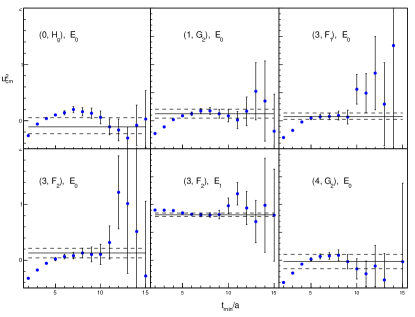
Figure 1: Variation of $t_{\mathrm{min}}$, the lower end of the range for single-exponential fits to the correlator ratio in Eq. 1. The vertical axis is the dimensionless center-of-mass momentum $u_{\mathrm{cm}}^{2}=L^{2}q^{2}_{\mathrm{cm}}/(2\pi)^{2}$. Shown here are the ground state energies from each of the five irreps $(\textbf{P}^{2},\Lambda)=\{(0,H_{g}),\,(1,G_{2}),\,(3,F_{1}),\,(3,F_{2}),\,(4,G_{2})\}$ and a single first excited state from the $(3,F_{2})$ irrep. For each fit $t_{\mathrm{max}}=25a$ while the dashed lines indicate the chosen fit.

Although multihadron correlation functions containing baryons are more computationally intensive than those with just mesons, the overall measurement cost is still dominated by the Dirac matrix inversions, which we perform efficiently using the DFL_SAP_GCR solver in openQCD oqc . However, the baryon functions defined in Eq. 23 of Ref. Morningstar et al. (2011) are the dominant storage cost.

Amplitude calculation: A variant of the methods of Refs. Lüscher (1991); Rummukainen and Gottlieb (1995) detailed in Refs. Göckeler et al. (2012); Morningstar et al. (2017) is applied to relate finite-volume $N-\pi$ energies to the infinite-volume elastic scattering amplitude. For each total momentum P and irrep $\Lambda$, these relations are given as determinant conditions of the form

$$\mathrm{det}(\hat{K}^{-1}-B^{(\textbf{P},\Lambda)})=0,$$ (2)

which hold up to exponentially suppressed residual finite volume effects. The determinant is taken over indices corresponding to the total angular momentum $J$, total orbital angular momentum $\ell$, total spin $S$, and an occurrence index $n$ labelling multiple occurrences of the partial wave in the irrep. The (infinite dimensional) matrix $B$ depends on the irrep and encodes the reduced symmetries of the finite volume. It is diagonal in $S$ but (in general) dense in all other indices. Expressions for all required elements of $B$ up to $J=13/2$ and $\ell=6$ are given in Ref. Morningstar et al. (2017). $\hat{K}$ is diagonal in $J$, equal to the identity in $n$, and is related to the usual $K$-matrix via $K_{\ell S;\ell^{\prime}S^{\prime}}^{-1}=q_{\mathrm{cm}}^{-(\ell+\ell^{\prime}+1)}\hat{K}_{\ell S;\ell^{\prime}S^{\prime}}^{-1}$ where $q_{\mathrm{cm}}$ is the center-of-mass momentum.

For this first calculation we only include irreps in which the $J^{\eta}=3/2^{+}$, $p$-wave is the lowest contributing partial wave Göckeler et al. (2012), namely $(\textbf{P}^{2},\Lambda)=\{(0,H_{g}),\,(1,G_{2}),\,(3,F_{1}),\,(3,F_{2}),\,(4,G_{2})\}$. In addition to ignoring the exponential finite volume effects in Eq. 2, contributions from higher $\ell>1$ are expected to be negligible based on threshold angular-momentum suppression. We assess the effect of this truncation to $\ell=1$ by performing a fit also including all $\ell=2$ contributions, namely the $J^{\eta}=3/2^{-}$ and $5/2^{-}$ partial waves. For this fit with the $\ell=2$ waves, we additionally include the ground state energy in the $(0,H_{u})$ irrep where the $3/2^{+}$ wave does not contribute, but both the $3/2^{-}$ and $5/2^{-}$ are present.

III Results

Results for the $I=3/2$, $p$-wave elastic $N-\pi$ scattering amplitude are presented in Fig. 2, where the (rescaled) real part of the inverse amplitude $(q_{\mathrm{cm}}/m_{\pi})^{3}\,\cot\delta_{\frac{3}{2}1}$ is shown as a function of the center-of-mass energy $E_{\mathrm{cm}}$. This quantity is smooth near the elastic $N-\pi$ threshold and, unlike the scattering phase shift, can describe both near-threshold resonances and bound states. However it is a highly nonlinear function of $E_{\mathrm{cm}}$, so that conventional horizontal and vertical error bars would be significantly correlated. Instead of these, in Fig. 2 for each energy we display one point for each of the central $68\%$ of bootstrap samples. This therefore gives a visual representation of the 1-$\sigma$ confidence interval for each point in this two-dimensional plot. Finally, in Fig. 2 $\tilde{E}_{\mathrm{cm}}=(E_{\mathrm{cm}}-m_{N})/m_{\pi}$ is shown on the horizontal axis so that the elastic region is given by $1<\tilde{E}_{\mathrm{cm}}<2$.

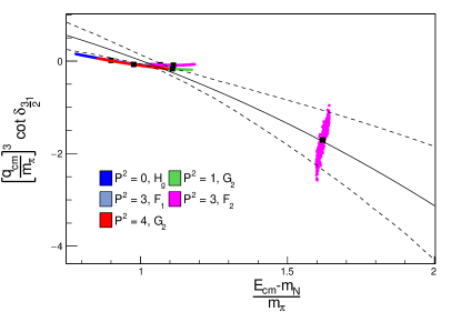
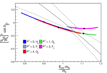
Figure 2: The real part of the inverse scattering amplitude for $I=3/2$, $p$-wave elastic $N-\pi$ scattering. Different colors indicate different energy levels, for each of which a colored circle is plotted for each of the central 68% of bootstrap samples and a black square indicates the mean value. The solid and dotted lines denote the mean values and bootstrap errors, respectively, for the Breit-Wigner fit described in the text. The lower panel focusses on the resonance region shown in the upper panel.

We describe the energy dependence of this amplitude with a Breit-Wigner shape

$$\left(\frac{q_{\mathrm{cm}}}{m_{\pi}}\right)^{3}\cot\delta_{\frac{3}{2}1}=\left(\frac{m^{2}_{\Delta}}{m^{2}_{\pi}}-\frac{E^{2}_{\mathrm{cm}}}{m_{\pi}^{2}}\right)\frac{6\pi E_{\mathrm{cm}}}{(g^{\mathrm{BW}}_{\Delta N\pi})^{2}m_{\pi}}$$ (3)

with fit parameters $m_{\Delta}/m_{\pi}$ and $g^{\mathrm{BW}}_{\Delta N\pi}$. The fit is performed using the method of Morningstar et al. (2017) in which the residuals in the correlated-$\chi^{2}$ are taken to be

$$\Omega(\mu,A)=\frac{\mathrm{det}(A)}{\mathrm{det}\left[(\mu^{2}+AA^{\dagger})^{1/2}\right]},$$

where $A=\hat{K}^{-1}-B^{(\textbf{P},\Lambda)}$ from Eq. 2. We take $\mu=1$, although fit parameters do not vary outside their statistical errors when going from $\mu=1$ to $\mu=10$.

The results of this fit (which neglects $\ell>1$ partial waves) are

$$\frac{m_{\Delta}}{m_{\pi}}=4.738(47),\quad g^{\mathrm{BW}}_{\Delta N\pi}=19.0(4.7),\quad\chi^{2}/\mathrm{d.o.f.}=1.11,$$

where the errors are statistical only. While our small number of data points makes fits to other parametrizations difficult, we can attempt to describe this partial wave in a nonresonant manner by truncating the effective range expansion at leading order, yielding the one-parameter fit form

$$\left(\frac{q_{\mathrm{cm}}}{m_{\pi}}\right)^{3}\cot\delta_{\frac{3}{2}1} =\frac{1}{m_{\pi}^{3}a_{{\frac{3}{2}1}}^{3}}.$$

This fit gives $(m_{\pi}a_{{\frac{3}{2}1}})^{-3}=-0.099(14)$ with $\chi^{2}/\mathrm{d.o.f.}=2.50$, indicating a poorer description of the data compared to the Breit-Wigner form of Eq. 3.

We can also assess the impact of the $3/2^{-}$ and $5/2^{-}$ $d$-waves which are present in the irreps with nonzero total momenta. In addition to the six energies included in the previous fits, we add the ground state in the total zero momentum $H_{u}$ channel, where these two waves are the lowest contributing partial waves. Although we only have seven energy levels, we nonetheless perform a four-parameter fit including the leading term in the effective range expansion for each of these additional waves

$$\left(\frac{q_{\mathrm{cm}}}{m_{\pi}}\right)^{5}\cot\delta_{\frac{3}{2}2}=\frac{1}{m_{\pi}^{5}a_{{\frac{3}{2}2}}^{5}},\quad\left(\frac{q_{\mathrm{cm}}}{m_{\pi}}\right)^{5}\cot\delta_{\frac{5}{2}2}=\frac{1}{m_{\pi}^{5}a_{{\frac{5}{2}2}}^{5}}$$

together with the parametrization of Eq. 3 for the $3/2^{+}$ $p$-wave. The results of this fit are

$$\frac{m_{\Delta}}{m_{\pi}}=4.734(56),\qquad g^{\mathrm{BW}}_{\Delta N\pi}=19.0(7.4),$$

$$(m_{\pi}a_{{\frac{3}{2}2}})^{-5}=0.00(10),\quad(m_{\pi}a_{{\frac{5}{2}2}})^{-5}=0.00(12),$$

$$\chi^{2}/\mathrm{d.o.f.}=4.17.$$

The values for $m_{\Delta}$ and $g^{\mathrm{BW}}_{\Delta N\pi}$ are consistent with those obtained from truncating to $\ell=1$, confirming our insensitivity to these $\ell=2$ waves.

Since $m_{N}/m_{\pi}=3.732(56)$, there is no significant difference between $m_{\Delta}$ and the elastic threshold at $E_{\mathrm{th}}/m_{\pi}=1+m_{N}/m_{\pi}$. By employing the scale determination of Ref. Bruno et al. (2017) we obtain a mass in physical units of $m_{\Delta}=1344(20)\mathrm{MeV}$, where the error on the scale has been combined in quadrature. It is worth emphasising that the quark masses for this ensemble are tuned to satisfy $\mathrm{Tr}M=2m_{l}+m_{s}=(\mathrm{Tr}M)^{\mathrm{phys}}$ as $m_{l}$ is lowered to its physical value, in contrast with the more standard choice where $m_{s}=m_{s}^{\mathrm{phys}}$ for all values of $m_{l}$.

Comparison of $g^{\mathrm{BW}}_{\Delta N\pi}$ can be made to experiment using the experimental values $m^{\mathrm{exp}}_{\Delta}\approx 1232\mathrm{MeV}$ and $\Gamma^{\mathrm{exp}}\approx 117\mathrm{MeV}$ from Ref. Patrignani et al. (2016) and the relation $\Gamma^{\mathrm{BW}}=\frac{(g^{\mathrm{BW}}_{\Delta N\pi})^{2}q_{\Delta}^{3}}{6\pi m_{\Delta}^{2}}$, where $q_{\Delta}$ is the center-of-mass momentum corresponding to the resonance mass. Such a comparison yields $g^{\mathrm{BW},\mathrm{exp}}_{\Delta N\pi}\approx 16.9$, in agreement with our result.

An alternative convention for the $\Delta N\pi$-coupling is provided by leading-order chiral effective theory Pascalutsa and Vanderhaeghen (2006), which defines $\Gamma$ as

$$\Gamma=\frac{(g^{\mathrm{LO}}_{\pi N\Delta})^{2}}{48\pi m_{N}^{2}}\frac{E_{N}+m_{N}}{E_{N}+E_{\pi}}q_{\Delta}^{3},$$

where $E_{N}$ and $E_{\pi}$ are the energies of the nucleon and pion, respectively, with momenta equal to $q_{\Delta}$. Using our calculated values for the resonance parameters and $m_{N}/m_{\pi}$ gives

$$g^{\mathrm{LO}}_{\pi N\Delta}=37.1(9.2).$$

Our result for $g^{\mathrm{LO}}_{\Delta N\pi}$ can be compared to previous lattice estimates using Fermi’s Golden Rule from Refs. Alexandrou et al. (2016, 2013), which give $g^{\mathrm{LO}}_{\Delta N\pi}=23.7(0.7)(1.1)$ at $m_{\pi}=180\mathrm{MeV}$ and $g^{\mathrm{LO}}_{\Delta N\pi}=26.7(0.6)(1.4)$ at $m_{\pi}=350\mathrm{MeV}$. We can also compare to a phenomenological extraction employing LO nucleon-pion effective field theory Pascalutsa and Vanderhaeghen (2006) yielding $g^{\mathrm{LO}}_{\Delta N\pi}=29.4(4)$, and a phenomenological $K$-matrix analysis Hemmert et al. (1995) yielding $g^{\mathrm{LO}}_{\Delta N\pi}=28.6(3)$.

IV Conclusions and outlook

This work presents the first lattice determination of meson-baryon resonance parameters directly from the scattering amplitude. It builds on demonstrably successful algorithms from the meson-meson sector Bulava et al. (2016), in particular the stochastic LapH method Morningstar et al. (2011), which reduces computational and storage costs for multihadron correlation functions containing baryons significantly compared to the distillation approach of Ref. Peardon et al. (2009).

The $I=3/2$, $p$-wave, elastic $N-\pi$ scattering amplitude is calculated here on a single ensemble of gauge configurations, and thus the usual lattice systematic errors due to finite lattice spacing and unphysical quark masses are not addressed. Furthermore while the magnitude of the exponentially suppressed finite volume effects indicated in Eq. 2 is presumably insignificant, this has not been checked explicitly.

This first analysis also avoids the influence of $\ell=0$ partial wave mixing in Eq. 2 by judiciously choosing irreps where this wave is absent and the $J=3/2$ $p$-wave is the leading contribution. Future work will include also irreps where the corresponding $s$-wave is present, which can be analyzed as described in Ref. Morningstar et al. (2017). These additional finite volume energies will better constrain the energy dependence of the amplitude and enable a more precise analysis of higher partial wave contributions. Furthermore, this calculation employs only a single permutation of stochastic quark line estimates. Additional ‘noise orderings’ may significantly improve the statistical precision.

Furthermore, these results will soon be complemented by measurements on other CLS ensembles. This will not only enable a check of the lattice spacing and (exponential) finite volume effects, but also elucidate the quark-mass dependence by using ensembles along the $\mathrm{Tr}M=\mathrm{const}.$ trajectory down to $m_{\pi}\lesssim 200\mathrm{MeV}$. While we have employed the ground states in each irrep and a single excited state from the $(3,F_{2})$ irrep here, at lighter pion masses, as $m_{\Delta}$ moves further above the elastic threshold, more excited states will also be included to provide additional points.

This first elastic $\Delta(1232)\rightarrow N\pi$ calculation may be viewed as a stepping stone in several respects. First, techniques for computing correlation functions, extracting finite volume energies, and analysing determinant conditions may be extended to other resonant meson-baryon systems. Such systems of interest may present additional complications like coupled scattering channels, as are present when studying the $\Lambda(1405)$ resonance. Finally, building upon this calculation of $\Delta(1232)\rightarrow N\pi$ will ultimately enable lattice QCD calculations of $\Delta(1232)$ transition form-factors, for which the theoretical foundations can be found in Ref. Agadjanov et al. (2014).