Relationship Profiling over Social Networks: Reverse Smoothness from Similarity to Closeness

Abstract.

On social networks, while nodes bear rich attributes, we often lack the ‘semantics’ of why each link is formed– and thus we are missing the ‘road signs’ to navigate and organize the complex social universe. How to identify relationship semantics without labels? Founded on the prevalent homophily principle, we propose the novel problem of Attribute-based Relationship Profiling (ARP), to profile the closeness w.r.t. the underlying relationships (e.g., schoolmate) between users based on their similarity in the corresponding attributes (e.g., education) and, as output, learn a set of social affinity graphs, where each link is weighted by its probabilities of carrying the relationships. As requirements, ARP should be systematic and complete to profile every link for every relationship– our challenges lie in effectively modeling homophily: We propose a novel reverse smoothness principle by observing that the similarity-closeness duality of homophily is consistent with the well-known smoothness assumption in graph-based semi-supervised learning– only the direction of inference is reversed. To realize smoothness over noisy social graphs, we further propose a novel holistic closeness modeling approach to capture ‘high-order’ smoothness by extending closeness from edges to paths. Extensive experiments on three real-world datasets demonstrate the efficacy of ARP.

1. Introduction

While our social universe– like our social lives– is complex, they are critically missing ‘road signs’ to navigate. On general networks like Twitter and DBLP, the edges (i.e. links, connections) between nodes (i.e. users) are often unlabeled– without ‘meanings.’ Even on more personal networks like Facebook and LinkedIn– where we spend much time everday interacting with friends in our ego networks– our connections with and between friends are lacking the ‘semantics’, in terms of the underlying relationships, e.g., schoolmate or colleague, resulting in cluttered social spaces and unorganized interactions. Such relationship semantics is crucial as ‘road signs’ to organize friends (Li et al., 2014; Sachan et al., 2014; Han and Tang, 2015) and route information (Chakrabarti et al., 2014; Rakesh et al., 2016; Yu et al., 2013) in our social universe. Without labeled connections, can we automatically identify the underlying relationships? This paper aims at such relationship profiling, in an unsupervised manner, which is important for modeling social networks.

Without pre-defined relationships, what ‘reasons’ do we give as the semantics for each link? With the well-known phenomenon of homophily (McPherson et al., 2001)– i.e., the tendency of individuals to stay close with similar others, it is often the case that a connection between users is a result of such tendency, i.e., it is formed due to their similarity in certain dimensions. Moreover, unlike existing works that consider homophily in a single dimension (Mislove et al., 2010; Şimşek and Jensen, 2008; Yang et al., 2011; Yang et al., 2017), we stress that homophily is naturally discriminative in that different relationships correspond to different dimensions of similarity, i.e., different attributes $\mathcal{A}$ lead to different relationships $\mathcal{R}$.

While no social network can capture all possible attributes and relationships, we observe that it is usually trivial to relate the most important relationships in a network to the particular attributes captured there. E.g., in a professional network like LinkedIn, the most important relationships are schoolmate and colleague, which are the result of similar education and employer attributes; on a personal network like Facebook, friends are formed through relationships such as townsmen and hobby peers resulted from their similarity in hometown and hobby. Table 1 gives more intuitive examples of important relationships $\mathcal{R}$ and relating attributes $\mathcal{A}$ on different networks.

Network	Important relationships and relating attributes
LinkedIn	$\mathcal{R}$	schoolmate	colleague	professional peer
	$\mathcal{A}$	education background	working experience	skill
Facebook	$\mathcal{R}$	townsman	hobby peer	acquaintance
	$\mathcal{A}$	hometown	sports, music, groups, etc.	check-ins, events, etc.
DBLP	$\mathcal{R}$	research group members	in-field collaborators	cross-field collaborators
	$\mathcal{A}$	publication	paper within the same fields	publication within different fields

Table 1. Some intuitive examples of relationships $\mathcal{R}$ and attributes $\mathcal{A}$ on different social networks.

We thus propose the problem of Attribute-based Relationship Profiling (ARP), founded on the principle of homophily– to profile the underlying relationships $\mathcal{R}$ of each connection by their associated attributes $\mathcal{A}$. While the problem is important, as social networks strives to help users organize their social universe and route information, it is also novel, and we are the first to identify it formally, to the best of our knowledge.

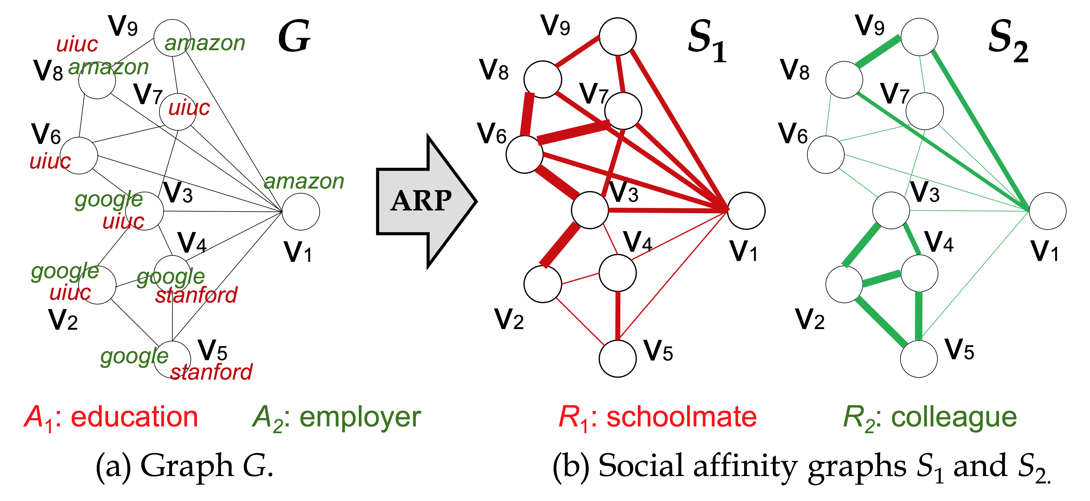
Figure 1. A toy example of a simple social network.

To illustrate, Figure 1(a) shows a network $\mbox{$\mathcal{G}$}=(\mbox{$\mathcal{V}$},\mbox{$\mathcal{E}$},\mbox{$\mathcal{A}$})$, where $\mathcal{V}$ is the set of nodes $v_{i}$ and $\mathcal{E}$ that of connections $e_{ij}$. $\mathcal{G}$ has a set of $M$ important attributes $\mbox{$\mathcal{A}$}=\{\mbox{$\mathcal{A}$}^{m}\}_{m=1}^{M}$ (e.g., $\mbox{$\mathcal{A}$}^{1}=$ education, $\mbox{$\mathcal{A}$}^{2}=$ employer) with the value functions, e.g., $\mbox{$\mathcal{A}$}^{1}(v_{8})=$ uiuc, $\mbox{$\mathcal{A}$}^{2}(v_{8})=$ amazon. Given $\mathcal{G}$ as input, ARP aims to profile $\mathcal{E}$ w.r.t. $\mathcal{A}$’s corresponding relationships $\mbox{$\mathcal{R}$}=\{\mbox{$\mathcal{R}$}^{m}\}_{m=1}^{M}$, by inferring its relationship probabilities $\{r^{m}_{ij}=p(e_{ij}|\mbox{$\mathcal{R}$}^{m},\mbox{$\mathcal{A}$}^{m})\}_{m=1}^{M}$, i.e., how each link $e_{ij}$ carries $\mathcal{R}$. As output, ARP constructs a set of social affinity graphs $\mbox{$\mathcal{S}$}=\{\mbox{$\mathcal{V}$},\mbox{$\mathcal{E}$},\mbox{$\mathcal{R}$}\}=\{\mbox{$\mathcal{S}$}^{m}\}_{m=1}^{M}$, i.e., graphs sharing the same structure of $\mathcal{G}$, where each link $e_{ij}$ in $\mbox{$\mathcal{S}$}^{m}$ is now weighted by $r^{m}_{ij}\in\mbox{$\mathcal{R}$}^{m}$ indicating how it carries $\mbox{$\mathcal{R}$}^{m}$. E.g., as Figure 1(b) shows, for $\mbox{$\mathcal{A}$}^{1}=$ education, ARP outputs the affinity graph $\mbox{$\mathcal{S}$}^{1}$ for $\mbox{$\mathcal{R}$}^{1}=$ schoolmate, and similarly, for $\mbox{$\mathcal{A}$}^{2}=$ employer, it outputs $\mbox{$\mathcal{S}$}^{2}$ for $\mbox{$\mathcal{R}$}^{2}=$ colleague. To visualize, we plot the thickness of a link to indicate its weight in $\mathcal{R}$.

We stress that, as the homophily principle implies, ARP should be ‘systematic’ and ‘complete’. On the one hand, individuals stay close because they are similar, and every link should have a probability to carry certain relationships. To this end, our profiling should be systematic to cover every link. E.g., two links ($e_{15}$ and $e_{19}$) may not carry a certain relationship (e.g., schoolmate, because it is weak or weaker than other relationships), but we may still want to compare them in that dimension. On the other hand, as similar individuals may stay close, more ‘similarity’ leads to more ‘closeness’, and any relationships can co-occur in a link. To this end, our profiling should be complete to cover every relationship on a link. E.g., two users ($v_{2}$ and $v_{3}$) may be both schoolmates and colleagues.

While natural, these dual requirements of homophily (and thus relationship semantics) have not been met by most existing works. Although the problem of ARP is novel, by similarly leveraging the homophily insight, several social mining methods have exploited relationship semantics as their intermediate results, but in a rather limited form– due to the failure to model homophily appropriately (Sec. 2): First, in attribute profiling works (Chakrabarti et al., 2014; Li et al., 2014; Tang and Liu, 2009; Yang et al., 2017), the homophily modeling is not complete, by restricting to one relationship per link. Second, in community detection works (Mcauley and Leskovec, 2012; Ruan et al., 2013; Yang et al., 2013, 2009), it is not systematic, by targeting at each community instead of links, which forces links in the same community to carry the same relationship, and leaves out those outside or between communities. As Sec. 6 will show, such improper models fall short for relationship profiling.

Thus, to address ARP, our key challenges center around effectively modeling homophily:

Challenge 1: Systematic and Complete Homophily.

As ARP requires, and as the nature of homophily implies, we should realize homophily over every link (systematicness) and for every relationship (completeness), which most existing work failed to satisfy. What is a principled mechanism for implementing homophily?

Insight: Reverse Smoothness Principle.

Over a graph, homophily bridges two kinds of ‘proximities’ between users, i.e., similarity, measuring how similar two users share for attributes $\mathcal{A}$, and closeness, measuring how close two users link through a relationship $\mathcal{R}$. Interestingly, we observe that, as this similarity-closeness duality is natural, it has been explored in graph-based semi-supervised learning (GSSL) (Zhou et al., 2004; Zhu and Ghahramani, 2002; Zhu et al., 2003). GSSL models the smoothness assumption, i.e., points close to each other are likely to share labels, which helps to infer from closeness (of links) to similarity (of labels) over a given, as input, data affinity graph, in a systematic (over every link) and complete (for every label) manner.

Surprisingly, while the smoothness assumption is remarkably consistent with homophily, their connection has only been exploited in a non-discriminative way that considers a unique relationship and mixes up all attributes (Yang et al., 2017). As our key insight is to leverage the modeling of smoothness to realize systematic and complete homophily, we note that our direction of inference for ARP is focused on the opposite to GSSL: from attributes to relationships. Therefore, we propose the reverse smoothness principle in Sec. 3 and a probabilistic model in Sec. 4, to infer from given similarity (of attributes $\mathcal{A}$) to latent closeness (of relationship $\mathcal{R}$) and construct, as output, a social affinity graph. We stress that, from similarity to closeness, the focus of ARP is exactly the opposite to that of GSSL– and this reverse smoothness has not been explored to date.

Challenge 2: Robust Homophily.

While the reverse smoothness principle allows us to relate attributes and relationships by implementing homophily, due to the incompleteness and ambiguity of attributes and links in real-world networks, similarity can not be computed and closeness can not be enforced directly between every pair of nodes. How to realize homophily robustly over such noisy social networks?

Insight: Holistic Closeness Modeling.

Traditional smoothness is only considered on direct edges between pairs of nodes by GSSL on the data affinity graph. It works because every edge exists and every pair-wise closeness is enumerated. In real-world networks where attributes are incomplete and ambiguous, and nodes with similar attributes do not always share an edge, such a scheme is useless.

To deal with real-world networks, we propose a holistic closeness modeling approach in Sec. 3 and implement it in Sec. 5, to leverage similarity between every pair of nodes– even though they may not have a direct link– by capturing the closeness between nodes based on paths, instead of edges. In other words, from edges to paths, we extend the traditional smoothness modeling to higher-order smoothness, so as to fully exploit the available attribute and link information on an incomplete ambiguous graph.

We intuitively explain the idea of this approach by continuing on the running example in Figure 1. It is intuitive to say that $e_{68}$ is very likely to carry relationship schoolmate, because $v_{6}$ and $v_{8}$ have the same education attribute. However, tricky questions arise due to the incomplete and ambiguous attributes. E.g., consider $e_{19}$, where neither of $v_{1}$ or $v_{9}$ has available education attribute, and $e_{23}$, where both $v_{2}$ and $v_{3}$ have multiple attributes. The holistic closeness modeling approach leverages paths that connect attributed nodes to profile edges they bypass. E.g., paths $v_{8}-v_{9}-v_{1}-v_{7}$ and $v_{5}-v_{2}-v_{3}-v_{4}$ bypass $e_{19}$ and $e_{23}$, respectively, so they add belief on $e_{19}$ to carry relationship schoolmate and $e_{23}$ to carry relationship colleague. In a nutshell, the approach exploits data redundancy in the neighborhood to complete and disambiguate relationships.

Summery.

In this paper, based on our novel reverse smoothness principle and holistic closeness modeling approach, we develop a probability framework of Attribute-based Relationship Profiling (ARP), which leverages user attributes and link structures to reliably estimate the proper relationship semantics in social networks. Specifically, we preserve reverse smoothness on the graph based on an interpretable probability experiment, and we achieve holistic modeling by measuring closeness through standard random walk. An efficient path finding algorithm is designed to solve our justifiable MLE objective. Finally, experiments on three real world datasets comprehensively demonstrate the effectiveness and efficiency of our ARP framework.

2. Related Work

As we discuss in Sec. 1, although we are the first to formally define the problem of ARP, since relationship semantics is critical for various tasks on social networks, algorithms in recent literature have already been intensively solving the related problems to ours. However, while they commonly believe in homophily and connect attributes and relationships with it, they do not correctly interpret the nature of homophily as complete and systematic. According to their main objectives, they can be categorized into two groups. The first group applies homophily to learn attributes through relationships, assuming that relationships on each link are mutually exclusive (Chakrabarti et al., 2014; Li et al., 2014; Tang and Liu, 2009). While they implicitly learn relationships, they do not compute the complete semantics on each link. The second group utilizes homophily to detect communities, assuming that each community of nodes are connected through the same relationships (Mcauley and Leskovec, 2012; Ruan et al., 2013; Yang et al., 2013, 2009). They compute the semantics of communities, rather than the systematic semantics on links.

The first group of algorithms can produce systematic but not complete relationship semantics. Since attribute learning aims to infer the missing attributes of every node, systematic relationship semantics can usually be retrieved afterwards by looking at the inferred attributes of nodes on each side of a link. The recent work EdgeExplain (Chakrabarti et al., 2014) is the closest to ours, which improves on traditional label propagation (Zhu and Ghahramani, 2002; Zhu et al., 2003) by modeling the interactions among different attributes and optimizing them jointly with relationships. However, it assumes that each link should only carry one relationship. The discriminative relational learning (Tang and Liu, 2009) exploits community features as latent social dimensions to aid attribute classification. Therefore, each link is only understood through one attribute chosen by the classification method applied on the two linked nodes. The Co-Profiling algorithm (Li et al., 2014) attempts to learn both user attributes and circles via searching for the reasons of link formation. Each link is then understood through one reason within one of the non-overlapping circles it detects. The BLA framework (Yang et al., 2017) differentiates links by attribute similarity between the connected nodes, but it does not assume multiple relationships on each link. Considering two users that are both colleagues and schoolmates, those algorithms force the result to be either of them, which is partial and does not always reflect the truth. In contrast, ARP will yield two close probabilities w.r.t. the two relationships.

The second group of algorithms can produce complete but not systematic relationship semantics. As they evolve, many community detection algorithms nowadays attempt to characterize communities through attributes. Examples include generative models like CESNA (Yang et al., 2013) and Circles (Mcauley and Leskovec, 2012) and other frameworks like PCL-DC (Yang et al., 2009) and CODICIL (Ruan et al., 2013). They all explicitly model the node attributes that cause communities to form and compute a weight matrix characterizing communities w.r.t. attributes. Relationship semantics can then be generated by assuming that links within the same communities carry the same relationships. Therefore, multiple relationships can be associated on each link, if the two linked nodes belong to multiple overlapping communities. However, since they only compute the community semantics, the relationship semantics computed from their results are coarse. To be more specific, there is no way to understand every link, such as those between different communities and outside of any communities. Moreover, they fail to distinguish individual links within the same community. Unlike them, ARP aims to profile relationships in a finer granularity. Rather than relying on the detection of communities, it utilizes the local paths to precisely understand every link as long as a path goes through it.

3. Motivation

In real-world networks, while links should bear different relationships, they are not explicitly labeled. We argue that being connected in a network does not mean being equally close in reality, and being close does not mean being equally close in every perspective. Since important relationships in social networks are usually discriminatively related with some particular attributes captured by the networks, we propose to leverage user attributes to decipher the hidden relationship semantics of uniform links.

Challenges.

The challenges of ARP, as discussed in Sec. 1, lie in the effective modeling of homophily– to be systematic and complete as well as robust. The former is difficult due to the lack of a principled way to infer relationships from attributes, and the later is hard because of missing and noisy information in real social networks.

Principle: Reverse Smoothness.

We notice that there is a systematic connection between attributes and relationships as we desire, which has been explored by the principled framework of graph-based semi-supervised learning (GSSL) (Zhou et al., 2004; Zhu et al., 2003). Specifically, GSSL models two proximities on the graph: closeness and similarity. Consider GSSL in the social network setting. For each user attribute $\mathcal{A}$, an affinity graph $\mathcal{R}$ is used to encode user closeness in terms of the corresponding relationship. Then the value of every user on $\mathcal{A}$ can be learned based on $\mathcal{R}$.

As an example, consider $v_{1}$, $v_{5}$ and $v_{6}$ in Figure 1(a). GSSL assumes that closeness in $\mathcal{R}$ is already given. Therefore, if $r_{16}$ is larger than $r_{15}$, the unknown education attribute of $v_{1}$ will be more likely to be predicted as $a_{6}$ (UIUC) than $a_{5}$ (Stanford), due to the following principle of GSSL.

Principle 1.

(Smoothness Principle) If two nodes $v_{i}$ and $v_{j}$ are close on the affinity graph $R$, their attributes $a_{i}$ and $a_{j}$ should be similar (Zhou et al., 2004; Zhu et al., 2003).

The focus of GSSL is thus on attribute inference, which goes from closeness to similarity on the graph.

Interestingly, the focus of ARP is the opposite of GSSL, i.e., from similarity to closeness. In ARP, e.g., we only know there is an edge $e_{13}$ between $v_{1}$ and $v_{3}$. We are interested in the closeness on $e_{13}$ in terms of schoolmate and colleague.

Inspired by GSSL, we intuitively reverse the smoothness principle into the following, which allows us to learn $\mathcal{R}$ by systematically enforcing closeness based on similarity, leading to a novel and unique solution to the ARP problem.

Principle 2.

(Reverse Smoothness Principle) If two users $v_{i}$ and $v_{j}$ share similar attributes on $\mathcal{A}$, they should be close on the social affinity graph in terms of  $\mathcal{R}$.

Based on this principle, it is intuitive to implement homophily by probabilistically estimating the closeness on every link in terms of each relationship $\mathcal{R}$ based on the similarity of its related attributes $\mathcal{A}$. The resulting social affinity graphs naturally encode the systematic and complete relationship semantics in the network.

Approach: Holistic Closeness Modeling.

Our situation in the real-world graph setting is more complex than that of GSSL. While GSSL can enumerate all pair-wise closeness on each edge and enforce similarity accordingly, the opposite is hard to do in social networks with missing and noisy information.

Firstly, attributes are incomplete. Consider $v_{1}$ and $v_{9}$ in Figure 1. Since the education attribute $a_{1}$ and $a_{9}$ are missing, we have no idea how similar they are, and thus how close $e_{19}$ should imply in terms of schoolmate. Moreover, even if attributes are complete, closeness cannot be simply enforced on every edge, because similarity can be ambiguous. This is due to the direction of inference, i.e., friends of relationship $\mathcal{R}$ must share the same related attribute $\mathcal{A}$, while similar in $\mathcal{A}$ does not necessarily mean close in $\mathcal{R}$. E.g., consider $v_{2}$ and $v_{3}$ in Figure 1. If $v_{2}$ and $v_{3}$ are schoolmates, they must share the same education attribute such as UIUC. However, sharing the same education attribute does not necessarily imply the relationship of schoolmates. In fact, they may be colleagues, because they also share the same employer attribute of Google, or both. If we simply enforce closeness on $e_{23}$, the results will be ambiguous.

To further leverage our reverse smoothness principle and robustly learn the social affinity graph $\mathcal{S}$, we propose to put smoothness constraints and closeness measures onto the whole graph, rather than limiting them to direct edges. Specifically, we define a path to be a sequence of non-repeating edges connecting two nodes and use reachability to measure closeness as a sum of all weighted paths between two nodes. Then we constrain closeness measured by reachability according to attribute similarity. The intuition is that, the more similar attributes $v_{i}$ and $v_{j}$ share, the closer they should be on the graph, and therefore the more paths of shorter lengths and larger weights should connect them.

Continue our example in Figure 1. Inferring $r_{19}$ in terms of schoolmate is challenging due to missing education attributes of $v_{1}$ and $v_{9}$. However, similarity between $v_{7}$ and $v_{8}$ can be used to estimate the closeness on path $v_{7}-v_{1}-v_{9}-v_{8}$, which indirectly estimates the closeness on $e_{19}$. As a result, $e_{19}$ is likely to carry relationship schoolmate, basically because $v_{1}$ and $v_{9}$ share many friends from UIUC such as $v_{7}$ and $v_{8}$.

Moreover, continue the discussion from Figure 1 about $v_{2}$ and $v_{3}$, where $e_{23}$ is ambiguous. If we combine closeness measured by multiple paths containing $e_{23}$, we will end up with a higher probability of $e_{23}$ to be formed due to Google rather than UIUC, mainly because of the short path $v_{4}-v_{3}-v_{2}-v_{5}$ containing $e_{23}$ between $v_{4}$ and $v_{5}$ with Google.

By constraining closeness measured by reachability on paths, we effectively utilize the constraints between each pair of nodes $v_{i}$ and $v_{j}$ with meaningful attributes onto all edges along the paths connecting $v_{i}$ and $v_{j}$, much beyond their direct edges, if any. Among those edges, many are likely to connect nodes without meaningful values of particular attributes, but in this way, they can still get properly constrained and thus well estimated. Moreover, since each edge can be a component of multiple constrained paths, multiple signals from nearby nodes are combined to disambiguate the semantics of that single edge, yielding more robust results.

4. Model

Maximizing the production of a similarity term and a closeness term is a standard way of preserving smoothness on the graph (Zhou et al., 2004; Zhu et al., 2003). However, the objective function is rather heuristically designed for optimization purposes and the scales of learned quantities are arbitrary.

The objective of ARP is to estimate a complete set of relationship probabilities systematically on each link. Moreover, this has to be done based on incomplete and ambiguous user attributes and link structures. We develop a unified probabilistic framework to derive the objective function of reverse smoothness and precisely learn the proper relationship probabilities through holistic closeness modeling.

We note that existing probabilistic models in graph-based settings only consider the inference from closeness to similarity on the comprehensive data affinity graphs, instead of the inference in the opposite direction on the incomplete and ambiguous social graphs as we consider (Fang et al., 2014; He et al., 2007; Subramanya and Bilmes, 2011).

4.1. Probabilistic Reverse Smoothness

To learn the systematic and complete relationship probabilities based on user attributes, we apply the reverse smoothness principle by designing a set of simulated probability experiments.

We start from the description of the probability space. Consider $M$ relationships in a network. We aim to learn one social affinity graph $\mbox{$\mathcal{S}$}^{m}$ by estimating its corresponding relationship probability matrix $R^{m}$ for each relationship. Since each connection can carry multiple relationships, we assume that $\{R^{m}\}_{m=1}^{M}$ follow the multinomial distribution on each existing connection and have $\forall i,j:\sum_{m=1}^{M}r^{m}_{ij}=1$.

To estimate $R^{m}$ based on user attributes, we model the closeness between users $v_{i}$ and $v_{j}$ on $\mbox{$\mathcal{S}$}^{m}$, by defining a user closeness event that $v_{i}$ and $v_{j}$ are close on the graph. We use a random variable $p^{m}(v_{i}\sim v_{j})$ to denote the probability of this event. In a simple case, user closeness can be directly represented by the relationship probability, i.e., $p^{m}(v_{i}\sim v_{j})=r^{m}_{ij}$.

Since we only observe attributes $\mathcal{A}^{m}$ directly from the network rather than the similarity $f^{m}(a_{i},a_{j})$, we firstly use intuitive examples to explain how to compute $f^{m}(a_{i},a_{j})$.

Consider $\mathcal{R}^{m}$ = schoolmate and $\mathcal{A}^{m}=$ university. For a single categorical attribute with multiple distinct values like this, a simple way to compute $f^{m}(a_{i},a_{j})$ is to assign 1 to it if $a_{i}$ and $a_{j}$ include at least one same value and 0 otherwise. This is basically doing the $or$ operations among the $and$ results between users on each distinct value of the specific attribute. For instance, if $v_{1}$ has attribute value UIUC, $v_{2}$ Stanford and $v_{3}$ both, then $a_{1}=(1,0)$, $a_{2}=(0,1)$, $a_{3}=(1,1)$ and $f^{m}(a_{1},a_{2})=0$ while $f^{m}(a_{1},a_{3})=f^{m}(a_{2},a_{3})=1$.

While we only consider a single categorical attribute towards each relationship in this work, it is trivial to generalize the framework to deal with multiple attributes and numerical attributes, which may help produce better attribute similarities. E.g., we can consider attributes like university and age for relationship schoolmates. For numerical attributes like age, We can normalize the difference among all users into $[0,1]$ by dividing the largest difference, and similarity then equals one minus the normalized difference. Then we can combine multiple attributes by simply applying a $min(\;)$ function on the similarities. Continue the example above, if user $v_{1}$ is 50 years old, $v_{2}$ is 23 and $v_{3}$ is 20, then we have $a_{1}=(1,0,50)$, $a_{2}=(0,1,23)$, $a_{3}=(1,1,20)$ and $f^{m}(a_{1},a_{2})=min(0,0.1)=0$, $f^{m}(a_{1},a_{3})=min(1,0)=0$ and $f^{m}(a_{2},a_{3})=min(1,0.9)=0.9$. The $min(\;)$ functions make sense because when we consider multiple attributes, we think users are similar only when they are similar in every perspective (e.g., schoolmates should be from the same university and of similar ages).

With a score $f^{m}(a_{i},a_{j})$ computed for each pair of users $v_{i}$ and $v_{j}$ describing their similarity on $\mathcal{A}^{m}$, we estimate their closeness in $\mathcal{R}^{m}$ in the following simulated probability experiments.

Each time, we pick up a pair of users $v_{i}$ and $v_{j}$ from the sample space $\Omega=\mathcal{V}^{2}$ according to $f^{m}(a_{i},a_{j})$ and observe that they are close on the graph. We require that the probability of randomly picking up $(v_{i}\sim v_{j})$ is proportional to $f^{m}(a_{i},a_{j})$. Therefore, considering a total number of $C$ relationships, after a sufficiently large number of experiments, the likelihood of observing the user closeness events is equivalent to

(1) $$L=\prod_{m=1}^{M}\prod_{i=1}^{N}\prod_{j=1}^{N}p^{m}(v_{i}\sim v_{j})^{f^{m}(a_{i},a_{j})}.$$

By maximizing $L$, we ensure that each pair of users are necessarily close on each social affinity graph $\mbox{$\mathcal{S}$}^{m}$ according to their attribute similarity in $\mathcal{A}^{m}$, while not too close under the constraints of multinomial distribution. Thus the objective of preserving reverse smoothness over the graph is fulfilled.

4.2. Holistic Closeness Modeling

As we discussed in Sec. 1 and 3, since attributes are incomplete and ambiguous on many users, closeness can not be directly enforced on every connection. To robustly estimate relationship probabilities, we develop a holistic model of user closeness based on random walks on graphs. While closeness can be asymmetric, we consider it in a symmetric way under the setting of undirected graphs. The framework generalizes trivially to directed graphs.

In this subsection, we derive the closeness model on one social affinity graph $\mathcal{S}$ and it is exactly the same for all other relationships. Therefore, we use $p$ interchangeably with $p^{m}$ in this subsection.

In standard random walks, edge weights $\mathcal{R}$ determine the one-step transition probabilities of the random walker on the graph, i.e., $p(v_{j}|v_{i})=\frac{r_{ij}}{d_{i}}$, where $d_{i}=\sum_{j\in\mathcal{N}(v_{i})}r_{ij}$ and $\mathcal{N}(v)$ is the set of nodes that share an edge with $v$ (Fang et al., 2014; Page et al., 1999). $p(v_{j}|v_{i})$ measures the edge-wise closeness on $\mathcal{S}$.

We propose to further measure path-wise (holistic) closeness. Consider a random walk on $\mathcal{S}$. Starting from a specific node $v_{i}$, besides jumping directly to $v_{j}$, the random walker can pass through several nodes between $v_{i}$ and $v_{j}$ with the corresponding transition probabilities before finally reaching $v_{j}$. The probability of the random walker to reach $v_{j}$ from $v_{i}$ through all possible paths accurately measures the holistic closeness between $v_{i}$ and $v_{j}$ on $\mathcal{S}$.

In order to capture and formalize holistic closeness, we bring out the notion of reachability in random walk (Lovász, 1993; Zhu et al., 2013):

(2) $$R(v_{i}\sim v_{j}) =\sum_{l\in l(v_{i}\sim v_{j})}r(l),$$

where $l(v_{i}\sim v_{j})$ is the set of all paths connecting $v_{i}$ and $v_{j}$, and $r(l)$ is the reachability through the specific path $l$ in a random walk. Although we focus on the reachability in only one direction, closeness is modeled symmetrically because we consider similarities in both directions equally.

Suppose all possible paths connecting $v_{i}$ and $v_{j}$ are known. We systematically enumerate reachability w.r.t. paths of different lengths and then add them up into a uniform representation. Specifically, we use $l_{kh}(v_{i}\sim v_{j})$ to denote the $h$th path of length $k$ between $v_{i}$ and $v_{j}$. Suppose $l_{kh}(v_{i}\sim v_{j})=v_{h_{1}}-v_{h_{2}}-\ldots-v_{h_{k+1}}$. At each step from $v_{h_{i}}$ to $v_{h_{i+1}}$, the transition probability is $\frac{r_{h_{i}h_{i+1}}}{d_{h_{i}}}$. We also consider the decay factor $\alpha$ to demote the impact of longer walks. Therefore, the reachability under the measure of $l_{kh}(v_{i}\sim v_{j})$ is

(3) $$p_{kh}(v_{i}\sim v_{j})=\alpha^{k}\prod_{s=1}^{k}\frac{r_{h_{s}h_{s+1}}}{d_{h_{s}}}.$$

In this form of multiplication, since the weight of the whole path is proportional to the weight of each edge and sub-path along that path, the closeness among nodes is naturally coupled and transmitted along the path.

Supposing there are totally $H$ paths of length $k$ connecting $v_{i}$ and $v_{j}$, then we have

(4) $$p_{k}(v_{i}\sim v_{j}) =\sum_{h=1}^{H}p_{kh}.$$

Considering all paths of different lengths between $v_{i}$ and $v_{j}$, we have

(5) $$p(v_{i}\sim v_{j}) =\sum_{k=1}^{K}p_{k},$$

where $K$ is the maximum length of paths we consider. To fully implement reachability as in Eq.2, $K$ should be set to $+\infty$. However, it is usually sufficient to set $K$ to small numbers like 3 or 4, due to the small world phenomenon, which makes longer paths less important (Watts and Strogatz, 1998). According to (Zhu et al., 2013), the ignored reachability on paths longer than K is bounded by $\alpha^{K+1}$, and in practice, we can dynamically increase $K$ to compute incremental reachability. In Sec. 6, we show the impact of different $\alpha$ and $K$.

Combing Eq.3, Eq.4 and Eq.5, we get the reachability between $v_{i}$ and $v_{j}$ measured by the whole graph as

(6) $$p(v_{i}\sim v_{j}) =\sum_{k=1}^{K}\sum_{h=1}^{H}\alpha^{k}\prod_{s=1}^{k}\frac{r_{h_{s}h_{s+1}}}{d_{h_{s}}}.$$

However, finding all possible paths connecting $v_{i}$ and $v_{j}$ is non-trivial. Therefore, an efficient path enumerating algorithm is devised especially for our scenario in Sec. 5.

4.3. Interpretation

We give an interpretation of how our probabilistic framework works in a random-walk perspective.

Combining Eq.1 and Eq.6, we get the likelihood function connecting path-wise user closeness with attribute similarity,

(7) $$L=\prod_{m=1}^{M}\prod_{i,j}(\sum_{k=1}^{K}\sum_{h=1}^{H}\alpha^{k}\prod_{s=1}^{k}\frac{r^{m}_{h_{s}h_{s+1}}}{d^{m}_{h_{s}}})^{f^{m}(a_{i},a_{j})}.$$

Consider a random walk on the graph. By constraining edge weights through path-wise closeness measured by reachability on the graph, we are actually requiring the random walker to ‘prefer’ paths connecting nodes with similar attributes, instead of always choosing an edge to go with uniform probabilities. This idea is similar to the supervised random walk in (Backstrom and Leskovec, 2011). But instead of generating ad hoc features for edges, we directly manipulate edge weights through paths, and thus the actual correspondence between edges and paths is leveraged.

As a result, for each edge or sub-path, the more paths connecting nodes with similar relating attributes pass through it, the more probable it will be visited by the random walker in the stationary distribution, and thus is more probable to be formed due to the relationship under consideration. Moreover, since there are many paths connecting each pair of attributed nodes and each path consists of multiple edges and sub-paths, many relationships among un-attributed nodes can be effectively profiled given only a few pairs of attributed nodes. Finally, all considered relationships compete on each connection due to the constraints of multinomial distribution, and the probability of each relationship to be carried on one connection is appropriately related to the number and distance of users with similar relating attributes around it. Thus the problems of missing and overlapping attributes are systematically addressed.

To show that our model essentially preserves reverse smoothness, we extract the generalized objective function of SSL as

(8) $$J_{SSL}=\sum_{m=1}^{M}\sum_{i,j}C^{m}_{ij}S^{m}_{ij},$$

where closeness (C) and similarity (S) are implemented in various ways due to different intuitions and measurements (Zhu and Ghahramani, 2002; Zhou et al., 2004; Lin et al., 2014). Maximizing Eq.8 with proper regularization essentially preserves smoothness by reducing the difference between C and S in M dimensions.

To contrast, we write the log-likelihood of ARP from Eq.7 as

(9) $$J_{ARP}=\sum_{m=1}^{M}\sum_{i,j}f^{m}(a_{i},a_{j})\log(\sum_{k=1}^{K}\sum_{h=1}^{H}\alpha^{k}\prod_{s=1}^{k}\frac{r^{m}_{h_{s}h_{s+1}}}{d^{m}_{h_{s}}}).$$

In this equation, $f(a_{i},a_{j})$ implements S while $\log(p(v_{i}\sim v_{j}))$ implements C. The correspondence between Eq. 8 and 9 indicates the effectiveness of ARP in preserving the reverse smoothness on the social affinity graph.

Note that, unlike Eq. 8 that is designed purely based on intuitions and optimization purposes, our Eq. 9 is derived from a principled probabilistic framework, where probability interpretation of relationship semantics is naturally preserved, and the coupling of closeness and similarity is decided by the well defined simulated probability experiments.

5. Algorithm

Realizing our holistic smoothness model is to compute a parameter configuration $\mathcal{R}$, so that the likelihood of observing the user closeness event is maximized according to attribute similarity. For this purpose, we need to firstly find relevant paths that can be constructed by existing edges on the graph, and then optimize weights $\mathcal{R}$ on them.

5.1. Finding Paths on Graph

According to Eq. 7, for each social affinity graph $\mathcal{S}$, we need to find paths $l(v_{i}\sim v_{j})$ for the pairs of nodes $v_{i}$ and $v_{j}$ with $f(a_{i},a_{j})>0$. Unlike traditional path enumeration on graphs, our problem is quite unique, where we only care about short paths between a small portion of nodes.

Since shorter paths contribute more in our model, we devise an efficient path finding algorithm based on breadth-first search (BFS), so that we can tune path length $K$ to avoid considering longer paths. In practice, $f(a_{i},a_{j})$ is usually very sparse, since there are numerous distinct values on $\mathcal{A}$ and many users do not have any meaningful value. Therefore, we only need to start from a very small number of nodes compared to $|\mathcal{V}|$. Finally, since we need to record the exact paths and avoid repeated iterations when considering the same nodes in different levels of search, we borrow the path descriptor $d(\cdot)$ from (Rubin, 1978) to encode, record and retrieve paths between nodes with time complexity $O(1)$. It is also efficient to check if a certain node or edge is on a path and if two paths are the same by simply doing binary AND and XOR on $d$.

Algorithm 1 formally demonstrates our novel path finding method. We evaluate its correctness by checking the completeness and non-repetitiveness. In Step 8, by requiring $v_{j}\notin l$, we require that the next node to be propagated to is not already in the path being considered, so no loopy paths can be generated; by requiring $l+e_{ij}\notin D(I,j)$, we guarantee that each path is generated only once. Moreover, in Step 10 and Step 14, we ensure that the same nodes are not considered multiple times in different search steps. Finally, in Step 6, we always consider every possible direction to make sure that no simple path is missed.

Since path indexing and legitimacy checking are efficiently $O(1)$ with the path descriptor lists, the overall computational complexity of finding paths is $O(K|\mathcal{V}|^{2})$. However, the actual computational time is much shorter than $K|\mathcal{V}|^{2}$. In each step of BFS, the numbers of considered nodes and neighbors are much less than $|\mathcal{V}|$. The efficiency of finding paths can be further improved by path caching and reusing, to fully utilize the path indexes. Specifically, we try to cache as many legitimate paths as possible after they are indexed. Therefore, the paths of length $K$ can be directly reused when considering paths longer than $K$. As the number of paths goes exponentially with the length of the paths, it is usually impossible to keep all path indexes in cache and even memory. Motivated by the scale-free property of social networks (Choromański et al., 2013), which leads to the frequent reuse of paths between a small number of high-degree hub nodes, we adopt the Least Recently Used (LRU) algorithm for path caching.

Algorithm 1 Efficient Path Finding Algorithm

1:procedure EPF $\triangleright$ Input $\mathcal{G}(\mathcal{V},\mathcal{E})$: the graph. $K$: the maximum length of paths we consider. $I$: the source node from which we want to find all paths to other nodes in the graph. $\triangleright$ Output $D(I,j),j=1\ldots|\mathcal{V}|$: each $D(I,j)$ is a list of path descriptors describing paths between $v_{I}$ and $v_{j}$. $\triangleright$ Variables we use $\Phi$: a bit vector of length $|\mathcal{V}|$, where $\Phi(i)$ marks if there is a sensor on node $v_{i}$. $\triangleright$ Initialize

2:     $\Phi(I)\leftarrow 1$, $\forall j\neq I,\Phi(j)\leftarrow 0$

3:     $\forall j,D(I,j)\leftarrow null$ $\triangleright$ Iteration

4:     for $k=1:K$ do

5:         for all $i$ in $1:|\mathcal{V}|$ with $\Phi(i)==1$ do

6:              for all $j$ in $1:|\mathcal{V}|$ with $e_{ij}==1$ do

7:                  for each path $l$ in $D(I,i)$ do

8:                       if $v_{j}\notin l\;\&\&\;l+e_{ij}\notin D(I,j)$ then

9:                           $D(I,j)=D(I,j)+(l+e_{ij})$

10:                           $\Phi(j)\leftarrow 1$

11:                       end if

12:                  end for

13:              end for

14:              $\Phi(i)\leftarrow 0$

15:         end for

16:     end for

17:     return $D(I,j),j=1\ldots|\mathcal{V}|$

18:end procedure

5.2. Optimizing Weights on Paths

Now that the paths connecting each pair of nodes with similar attributes are found, we continue to optimize the log-likelihood function in Eq.7 and generate the relationship probabilities $\mathcal{R}$. We derive the gradient for $r_{uv}$ as

(10) $$\frac{\partial J}{\partial r^{m}_{uv}} =\sum_{i,j}f_{m}(a_{i},a_{j})\frac{N_{uv}(v_{i}\sim v_{j})}{p_{m}(v_{i}\sim v_{j})}.$$

In the equation,

(11) $$N^{m}_{uv}(v_{i}\sim v_{j})=\sum_{k=1}^{K}\sum_{h=1}^{H}I\{l_{kh},e_{uv}\}\frac{p^{m}_{kh}(v_{i}\sim v_{j})}{r^{m}_{uv}},$$

where $I\{l_{kh},e_{uv}\}$ is an indicator function computed from path $l_{kh}$. Specifically, $I\{l_{kh},e_{uv}\}$ equals 1 if $l_{kh}$ contains edge $e_{uv}$, and 0 otherwise. Therefore, $N^{m}_{uv}(v_{i}\sim v_{j})$ is the sum of the products of all normalized edge weights except for $r^{m}_{uv}$ along all paths that connect nodes $v_{i}$ and $v_{j}$ and also contain edge $e_{uv}$.

With Eq.10, we apply standard gradient ascent to solve for $\mathcal{R}$. As can be seen in Eq.11, for a specific edge $e_{uv}$, the more paths $l_{kh}$’s pass through it ($I\{l_{kh},e_{uv}\}$ equals 1), the larger the derivative of the corresponding weight $r^{m}_{uv}$ is, which substantiates our intuition of using paths connecting similarly attributed nodes to profile individual edges. In Eq.3, the denominator $d_{h_{s}}$ exposes an $l$-1 norm on all weights in $\mathcal{R}^{m}$, encouraging sparse solutions. The penalty arises naturally within the probabilistic model and therefore no heuristic penalty terms to encourage sparsity is necessary.

Consider a specific pair of nodes $v_{i}$ and $v_{j}$. Given Eq.3, $p_{kh}(v_{i}\sim v_{j})$ is concave in $\mathcal{R}$. Moreover, since different paths connecting $v_{i}$ and $v_{j}$ found by our algorithm never share the same edge, $p_{k}(v_{i}\sim v_{j})$ and $p(v_{i}\sim v_{j})$ in Eq.4 and Eq.5 are both concave in $\mathcal{R}$. Since log concave is still concave, the log-likelihood function in Eq.6 is a weighted sum of concave functions, which is not globally concave but has an upper bound. However, since $f(a_{i},a_{j})$’s are usually very sparse in social networks, we find the solution of our algorithm stable and almost always the global optimal in the experiments.

The runtime of ARP is dominated by finding paths. The runtime of optimization with gradient ascent is linear in $|\mathcal{V}|$. As we study in our experiments, convergence is reached usually within 20 iterations with step size empirically set to 0.05. As discussed before, the time of finding paths is much less than $K|\mathcal{V}|^{2}$, so the overall time complexity of ARP is $O(K|\mathcal{V}|^{2})$, comparable to many advanced attribute profiling and community detection algorithms (Chakrabarti et al., 2014; Li et al., 2014; Mcauley and Leskovec, 2012).

6. Experiments

In this section, we evaluate ARP with quantitive experiments and case studies on three real-world datasets.

6.1. Experimental Settings

Datasets.

The first is the LinkedIn Ego Networks dataset (LEN) from (Li et al., 2014). It includes 268 ego networks, which contain about 19K users and 110K connections. Among them, about 30% users have attributes of 193 different universities and 375 different employers. 8K connections are labeled by the ego users as carrying the relationships of schoolmates, colleagues or both, based on which we directly perform quantitive performance evaluations.

The second is the Facebook Ego Networks dataset (FEN) from (Mcauley and Leskovec, 2012). It contains 10 ego networks of about 4K users and 88K connections. We choose all hometown, school and employer attributes out from the total 634 attributes, because they well indicate the relationships of townsman, schoolmate and colleague. Since there are no labeled relationships, we randomly split the users into training and testing sets. We input all users with their connections and attributes in the training set to all compared algorithms, and evaluate the learned relationships on connections between users in the training set and users in the testing set. For quantitive evaluations, we label the relationship of townsman (schoolmate, colleague) on the connections between friends sharing the same attribute value of hometown (school, employer). Thus, there might be multiple relationships on the same connection.

The DBLP data we use were extracted on Jan 1st, 2017, which includes 3.7M publications from 1.8M authors. We generate nodes as authors and use three publication venues, KDD, VLDB and ICML, as node attributes. A uniform connection is generated between authors who have co-authored at least once in any of the considered venues. Since the authors and attributes are not anonymous, we present insightful case study results on some novel applications to show the effectiveness of our framework.

The attributes captured in both LEN and FEN are incomplete and noisy. In such scenarios, we show that profiling the systematic and complete relationship semantics is generally useful in improving the performance of relationship prediction. Although both LEN and FEN are ego-networks, our framework is general to work on any non-ego-networks like DBLP. Moreover, on DBLP where the attributes are complete and precise, we show that our framework is still advantageous because it provides more insightful results.

Compared algorithms.

The problem of ARP is novel, which is hardly addressed by previous literature. As discussed in Sec. 2, to comprehensively evaluate ARP, we adapt state-of-the-art algorithms from two groups.

Adapting attribute profiling algorithms.

These algorithms aim at inferring user attributes based on both known attributes and network structure. Since the relationships they learn are implicit, we need to predict them based on the inferred attributes on the connected users. E.g., we predict a relationship as schoolmate if the two connected users are inferred with the same university attributes.

• Relation neighbor classifier (RNC) (Macskassy and Provost, 2003): it profiles user attributes w.r.t. labeled neighbors without learning.

• Discriminative relational classifier (DRC) (Tang and Liu, 2009): it constructs a modularity-based feature as latent social dimensions to help learn user attributes.

• EdgeExplain (Chakrabarti et al., 2014): it improves on traditional label propagation (Zhu and Ghahramani, 2002; Zhu et al., 2003) by leveraging a softmax function to solve for a global optimal assignment of both user attributes and relationships.

• BLA (Yang et al., 2017): it jointly infers link and attribute probabilities by addressing smoothness from two directions on social graphs.

Adapting community detection algorithms.

We adapt community detection algorithms that use node attributes to characterize communities, which have a side effect of profiling links at a coarse granularity. We refer to the attribute assignment of each community and predict all relationships based on the most prominent attribute. E.g., we predict all relationships in a community as schoolmate if a university attribute is the most prominent there.

• PCL-DC (Yang et al., 2009): it unifies a conditional model for link and a discriminative model for content analysis.

• Circles (Mcauley and Leskovec, 2012): it designs a generative model of edges w.r.t. profile similarity to detect overlapping communities.

• CESNA (Yang et al., 2013): it designs a generative model of edges and attributes to detect overlapping communities.

• CoProfiling (Li et al., 2014): it profiles attributes and community memberships through iterative coordinate descent.

Instead of producing a set of relationship probabilities for each link like ARP, all baselines can only produce categorical labels.

Metrics.

For performance evaluations, we compute precision, recall and F1 score over all predictions of each relationship as commonly done in related works (Li et al., 2014). The presented results are the averages over 10 times of the same procedures. We also conduct significance tests with $p$-value 0.01.

To further understand the results, we evaluate the relationships profiled by different algorithms w.r.t. the systematicness and completeness criteria as we discussed in Sec. 1. We compute the number of all links in the network ($E$), the number of profiled links ($P$) and the number of links profiled with multiple relationships ($M$). To measure the systematicness, we compute $S=P/E$, and to measure completeness, we compute $C=M/P$.

We also measure the actual runtimes of different algorithms on a typical PC with dual 2.3 GHz Intel i7 processors and 8GB memory.

6.2. Performance Comparison on LEN

On the LEN dataset, ARP is quantitively evaluated against all baselines. Given a uniform social network, the task is to identify relationships that are discriminatively related to user attributes. Here we aim to identify schoolmates, who are likely to share the same university attributes, and colleagues, who are likely to share the same employer attributes. Evaluation is done on the user labeled relationships.

We run ARP on the university and employer attributes and predict the probabilities of schoolmate and colleague relationships on each link. To perform quantitive evaluations, we convert the probabilities into binary predictions for each relationship by thresholding at value $\theta^{m}$. For attribute learning algorithms, we predict schoolmates if the two connected users are inferred with the same university attribute; for community detection algorithms, we predict schoolmates if a certain university is the most prominent attribute for the detected community that contains both connected users. The same is done to predict colleagues.

We select the best parameters for all algorithms via standard 5-fold cross validation. The parameters we set for ARP are $K=3$, $\alpha=0.8$, $\theta^{1}=0.4$ and $\theta^{2}=0.7$.

Algorithm	Schoolmates			Colleagues
	P	R	F1	P	R	F1
RNC	0.613	0.548	0.579	0.358	0.467	0.405
DRC	0.885	0.472	0.616	0.603	0.442	0.510
EdgeExplain	0.782	0.618	0.690	0.530	0.642	0.581
BLA	0.648	0.683	0.665	0.416	0.697	0.521
PCL-DC	0.932	0.498	0.649	0.654	0.516	0.577
Circles	0.937	0.431	0.590	0.512	0.428	0.466
CESNA	0.813	0.492	0.613	0.502	0.538	0.519
CoProfiling	0.969	0.487	0.648	0.691	0.453	0.547
ARP	0.941	0.793	0.861	0.705	0.782	0.742

Table 2. Performance comparison on LEN.

Table 2 shows performance comparison on LEN. The scores all passed the significance tests with p-value 0.01. ARP constantly ranks first among the 8 algorithms on F1 score, while other methods have varying performance, which indicates the robustness and universal advantages of our approach on precisely profiling individual links. By looking into the scores, we find that ARP can effectively improve recall, while maintaining comparable precision to the baselines. It shows the effectiveness of our model to systematically and completely profile relationships along paths connecting users with similar attributes.

We present systematicness and completeness evaluations in Table 3, where the ratios are averaged through 10 random training-testing splits. As clearly shown, the attribute profiling algorithms usually profile only one relationship for every connection, while the community detection algorithms predict no relationship at all on some connections. ARP is the only one that implements systematic and complete homophily by profiling every connection w.r.t. every relationship.

Algorithm	RNC/DRC	EdgeExplain	BLA	PCL-DL
Systematicness	100%	100%	100%	88.7%
Completeness	0%	15.7%	78.2%	64.0%
Algorithm	Circles	CESNA	CoProfiling	ARP
Systematicness	83.6%	86.2%	91.4%	100%
Completeness	81.2%	72.9%	0%	100%

Table 3. Systematicness and completeness of relationships profiled by different algorithms on LEN.

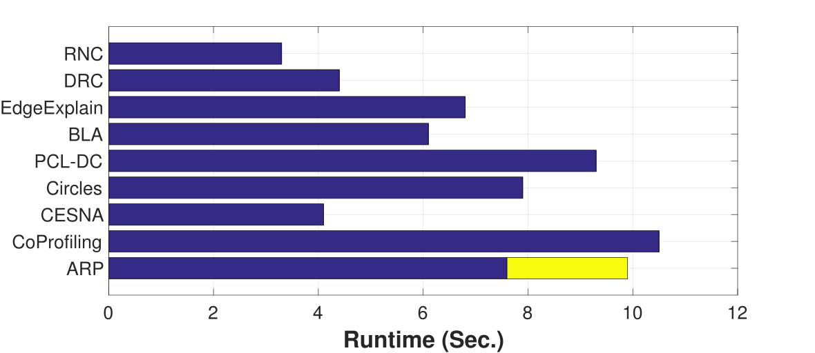
Figure 2. Runtime comparison on LEN.

We present the average runtime of different algorithms on LEN in Figure 2. For ARP, we compare the runtime with and without path caching and reusing, as discussed in Sec. 5 (the additional runtime without path caching is marked as yellow). The runtime of ARP is comparable to the baselines.

6.3. Performance and Parameter Study on FEN

We run experiments on FEN with varying portions of training and testing sets to comprehensively evaluate the performance of ARP. We also closely study the impact of the two intrinsic parameters of ARP, i.e., $\alpha$, the decay factor, and $K$, the maximum length of paths we consider.

To compute the F1 scores, the similar process for LEN has been done to all compared algorithms to yield a binary prediction for each of the townsman, schoolmate and colleague relationships on each connection.

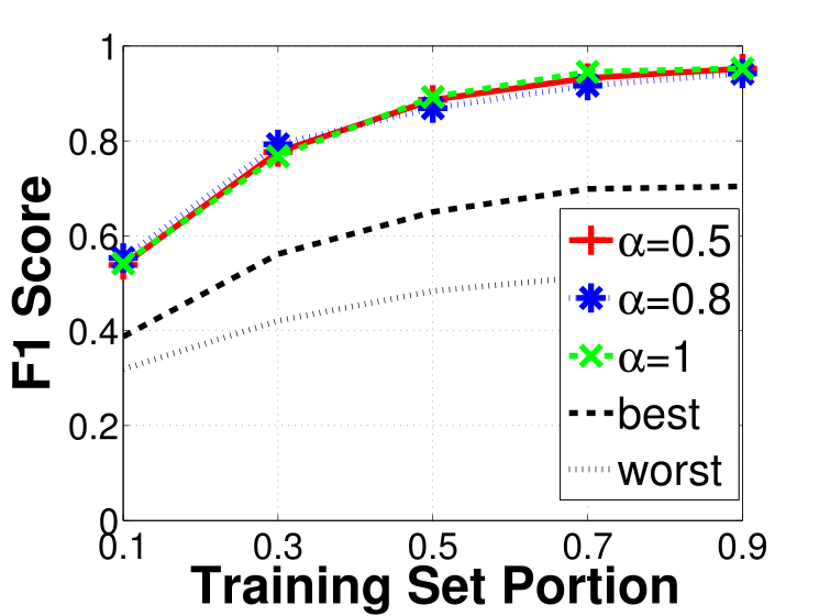
(a) Varying $\alpha$ while $K=3$

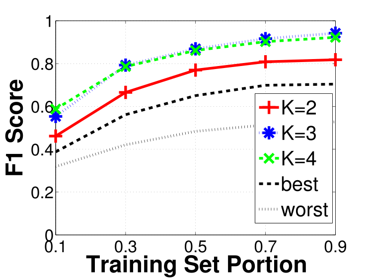
(b) Varying $K$ while $\alpha=0.8$

Figure 3. Performance study with baselines on FEN.

Figure 3 shows experimental results on FEN for townsman with $\theta^{1}=0.2$. The results for schoolmates and colleagues are similar. In Figure 3(a), the decay factor $\alpha$ does not significantly influence the performances. This is probably because we only consider short paths. In Figure 3(b), when $K$ is set to 2, only two-step paths are considered, which leads to quite poor results. When $K$ is set to larger values like 3 and 4, the holistic modeling approach becomes effective and the results are much better. Note that $K=3$ and $K=4$ always yield similar results, which indicates that the importance of paths is dominated by short ones. By setting $K$ to small values like 3, we can run ARP efficiently by avoiding irrelevant edges.

6.4. Case Study on DBLP

One advantage of ARP over the compared algorithms is that it can estimate the probability of each connection to carry each relationship. On LEN and FEN, we convert the probabilities into binary outputs in order to present quantitive comparisons with the baselines. However, the application of ARP is much broader than binary predictions. We use DBLP to present some insightful results derived from the relationship probabilities, which only ARP can generate.

Consider some interesting novel applications on DBLP. One of them is to find out people’s closest co-authors within different research fields. E.g., two authors might study similar problems in data mining, but very different problems in database. Thus, how can we identify people’s closest co-authors given a specific field? Another interesting application is to identify the closest pairs of authors within each field of study, i.e., who study the closest problems and collaborate most in a specific field? Considering specific relationships, such problems are novel and naturally different from general graph ranking.

We show that problems like these are direct applications of ARP. By modeling publication venues as user attributes and co-authorship as user connections, ARP accurately computes the closeness among authors w.r.t. different fields.

Consider three representative venues that correspond to three different but related fields. Table 3 shows the relationship specific closeness learned by ARP and normalized into multinomial distributions over each pair of authors. While relationships can be multiple and vary across connections, ARP completely retrieves them in all aspects.

Authors	KDD	VLDB	ICML
Jiawei Han, Philip S. Yu	0.65	0.35	0
Jiawei Han, Xiaolei Li	0.04	0.96	0
Jiawei Han, Tianbao Yang	0.17	0	0.83
Christos Faloutsos, Hanghang Tong	0.86	0.13	0.01
Divesh Srivastava, H. V. Jagadish	0.03	0.97	0
Corinna Cortes, Mehryar Mohri	0.14	0	0.86

Table 4. Multi-aspect relationships among authors.

Authors	(A) Holistic	(B) Single
Jiawei Han, Chi Wang	1.00/1st	1.00/1st
Christos Faloutsos, Hanghang Tong	0.95/2nd	1.00/1st
Hynne Hsu, Mong-Li Lee	0.93/3rd	0.72/10th
Jiawei Han, Philip S. Yu	0.90/4th	0.63/18th
Christos Faloutsos, Lei Li	0.85/5th	0.72/10th

Table 5. Rank list of closest authors on KDD.

In Table 4, pairs of authors are ranked with their relative closeness in the research field of data mining w.r.t. the KDD conference. Column (A) shows the results of holistic modeling, where we set $K=3$ and $\alpha=0.8$ to consider indirect collaborations. The results are intuitive because the top ranked pairs of authors are indeed those who collaborate most in the field. To show that the results in Column (A) are non-trivial as cannot be simply computed by counting the number of collaborated papers, we also provide in Column (B) the results without holistic modeling, which are less intuitive. E.g., although Han and Yu work quite closely on data mining, the closeness between them decreases from 0.90 to 0.63 and their rank drops from $4th$ to $18th$, merely because their many indirect collaborations are ignored. The situations are similar for many other pairs such as Faloutsos and Li.

Due to space limit, please refer to our anonymous Github project to explore more interesting novel applications and visualizations enabled by ARP. The codes are also available under the same directory.

7. Conclusion

While ARP is a novel problem that can be viewed as an essential part of problems such as attribute learning and community detection, we emphasize that this problem itself is important, complex and of great research value. As a unique solution, we propose to learn relationship semantics in a principled probabilistic way, which characterizes the formation of each user connection in social networks based on user attributes. Since ARP enables automatic labeling of relationships in an unsupervised way, the roles that different relationships play in various networks can be rigorously studied, such as promoting certain messages and shaping specific groups.

References

- (1)
- Backstrom and Leskovec (2011) Lars Backstrom and Jure Leskovec. 2011. Supervised random walks: predicting and recommending links in social networks. In WSDM. 635–644.
- Chakrabarti et al. (2014) Deepayan Chakrabarti, Stanislav Funiak, Jonathan Chang, and Sofus Macskassy. 2014. Joint Inference of Multiple Label Types in Large Networks. In ICML. 874–882.
- Choromański et al. (2013) Krzysztof Choromański, Michał Matuszak, and Jacek Mi?kisz. 2013. Scale-free graph with preferential attachment and evolving internal vertex structure. Journal of Statistical Physics 151, 6 (2013), 1175–1183.
- Fang et al. (2014) Yuan Fang, Kevin Chen-Chuan Chang, and Hady Wirawan Lauw. 2014. Graph-based Semi-supervised Learning: Realizing Pointwise Smoothness Probabilistically. In ICML.
- Han and Tang (2015) Yu Han and Jie Tang. 2015. Probabilistic community and role model for social networks. In Proceedings of the 21th ACM SIGKDD International Conference on Knowledge Discovery and Data Mining. ACM, 407–416.
- He et al. (2007) Jingrui He, Jaime G Carbonell, and Yan Liu. 2007. Graph-Based Semi-Supervised Learning as a Generative Model.. In IJCAI, Vol. 7. 2492–2497.
- Li et al. (2014) Rui Li, Chi Wang, and Kevin Chen-Chuan Chang. 2014. User profiling in an ego network: co-profiling attributes and relationships. In WWW. 819–830.
- Lin et al. (2014) Binbin Lin, Ji Yang, Xiaofei He, and Jieping Ye. 2014. Geodesic Distance Function Learning via Heat Flow on Vector Fields. In ICML.
- Lovász (1993) László Lovász. 1993. Random walks on graphs: A survey. Combinatorics, Paul erdos is eighty 2, 1 (1993), 1–46.
- Macskassy and Provost (2003) Sofus A Macskassy and Foster Provost. 2003. A simple relational classifier. Technical Report. DTIC Document.
- Mcauley and Leskovec (2012) Julian J Mcauley and Jure Leskovec. 2012. Learning to discover social circles in ego networks. In NIPS. 539–547.
- McPherson et al. (2001) Miller McPherson, Lynn Smith-Lovin, and James M Cook. 2001. Birds of a feather: Homophily in social networks. Annual review of sociology (2001), 415–444.
- Mislove et al. (2010) Alan Mislove, Bimal Viswanath, Krishna P Gummadi, and Peter Druschel. 2010. You are who you know: inferring user profiles in online social networks. In WSDM. 251–260.
- Page et al. (1999) Lawrence Page, Sergey Brin, Rajeev Motwani, and Terry Winograd. 1999. The PageRank citation ranking: Bringing order to the web. (1999).
- Rakesh et al. (2016) Vineeth Rakesh, Wang-Chien Lee, and Chandan K Reddy. 2016. Probabilistic Group Recommendation Model for Crowdfunding Domains. In Proceedings of the Ninth ACM International Conference on Web Search and Data Mining. ACM, 257–266.
- Ruan et al. (2013) Yiye Ruan, David Fuhry, and Srinivasan Parthasarathy. 2013. Efficient community detection in large networks using content and links. In WWW. 1089–1098.
- Rubin (1978) Frank Rubin. 1978. Enumerating all simple paths in a graph. ITCS 25, 8 (1978), 641–642.
- Sachan et al. (2014) Mrinmaya Sachan, Avinava Dubey, Shashank Srivastava, Eric P Xing, and Eduard Hovy. 2014. Spatial compactness meets topical consistency: jointly modeling links and content for community detection. In Proceedings of the 7th ACM international conference on Web search and data mining. ACM, 503–512.
- Şimşek and Jensen (2008) Özgür Şimşek and David Jensen. 2008. Navigating networks by using homophily and degree. Proceedings of the National Academy of Sciences 105, 35 (2008), 12758–12762.
- Subramanya and Bilmes (2011) Amarnag Subramanya and Jeff Bilmes. 2011. Semi-supervised learning with measure propagation. Journal of Machine Learning Research 12, Nov (2011), 3311–3370.
- Tang and Liu (2009) Lei Tang and Huan Liu. 2009. Relational learning via latent social dimensions. In Proceedings of the 15th ACM SIGKDD international conference on Knowledge discovery and data mining. ACM, 817–826.
- Watts and Strogatz (1998) Duncan J Watts and Steven H Strogatz. 1998. Collective dynamics of small-world networks. nature 393, 6684 (1998), 440–442.
- Yang et al. (2017) Carl Yang, Lin Zhong, Li-Jia Li, and Luo Jie. 2017. Bi-directional Joint Inference for User Links and Attributes on Large Social Graphs. In Proceedings of the 26th International Conference on World Wide Web Companion. 564–573.
- Yang et al. (2013) Jaewon Yang, Julian McAuley, and Jure Leskovec. 2013. Community detection in networks with node attributes. In ICDM. 1151–1156.
- Yang et al. (2011) Shuang-Hong Yang, Bo Long, Alex Smola, Narayanan Sadagopan, Zhaohui Zheng, and Hongyuan Zha. 2011. Like like alike: joint friendship and interest propagation in social networks. In WWW. 537–546.
- Yang et al. (2009) Tianbao Yang, Rong Jin, Yun Chi, and Shenghuo Zhu. 2009. Combining link and content for community detection: a discriminative approach. In SIGKDD. 927–936.
- Yu et al. (2013) Xiao Yu, Xiang Ren, Yizhou Sun, Bradley Sturt, Urvashi Khandelwal, Quanquan Gu, Brandon Norick, and Jiawei Han. 2013. Recommendation in heterogeneous information networks with implicit user feedback. In Proceedings of the 7th ACM conference on Recommender systems. ACM, 347–350.
- Zhou et al. (2004) Dengyong Zhou, Olivier Bousquet, Thomas Navin Lal, Jason Weston, and Bernhard Schölkopf. 2004. Learning with local and global consistency. NIPS 16, 16 (2004), 321–328.
- Zhu et al. (2013) Fanwei Zhu, Yuan Fang, Kevin Chen-Chuan Chang, and Jing Ying. 2013. Incremental and accuracy-aware personalized pagerank through scheduled approximation. VLDB 6, 6 (2013), 481–492.
- Zhu and Ghahramani (2002) Xiaojin Zhu and Zoubin Ghahramani. 2002. Learning from labeled and unlabeled data with label propagation. Technical Report. Citeseer.
- Zhu et al. (2003) Xiaojin Zhu, Zoubin Ghahramani, John Lafferty, and others. 2003. Semi-supervised learning using gaussian fields and harmonic functions. In ICML, Vol. 3. 912–919.