Multi-dimensional Tensor Network Simulation of Open Quantum Dynamics in Singlet Fission

Abstract

We develop a powerful tree tensor network states method that is capable of simulating exciton-phonon quantum dynamics of larger molecular complexes and open quantum systems with multiple bosonic environments. We interface this method with ab initio density functional theory to study singlet exciton fission (SF) in a pentacene dimer. With access to the full vibronic many-body wave function, we track and assign the contributions of different symmetry classes of vibrations to SF and derive energy surfaces, enabling us to dissect, understand, and describe the strongly coupled electronic and vibrational dynamics, relaxation, and reduced state cooling. This directly exposes the rich possibilities of exploiting the functional interplay of molecular symmetry, electronic structure and vibrational dynamics in SF material design. The described method can be similarly applied to other complex (bio-) molecular systems, characterised by a rich manifold of electronic states and vibronic coupling driving non-adiabatic dynamics.

Ultrafast open quantum dynamics have recently attracted considerable attention in the context of molecular light harvesting materials, where experimental evidence has begun to highlight the role of coherent, non-equilibrium vibronic dynamics in systems ranging from organic photovoltaics to the pigment-protein complexes of photosynthesis Brédas et al. (2017); Romero et al. (2017). Exploiting this complex interplay of vibrational and electronic quantum dynamics in tailored materials offers an exciting route towards advanced, next-generation light harvesting devices Scholes et al. (2017), and the process known as singlet fission (SF) has recently been shown to be a very promising area in which to explore this.

In organic semiconductors such as pentacene, a photogenerated singlet exciton undergoes singlet fission into a pair of entangled triplet excitons on sub-$100\,\mathrm{fs}$ timescales, efficiently generating two electronic excitations from a single incoming photonSmith and Michl (2013); Berkelbach et al. (2013a). Harnessing this potential carrier multiplication could help to overcome the Shockley-Queisser limit in photovoltaics Shockley and Queisser (1961), and understanding the links between the dynamics and efficiency of SF has emerged as an active interdisciplinary field of research Wilson et al. (2013); Walker et al. (2013); Yost et al. (2014); Alguire et al. (2015); Tamura et al. (2015); Zheng et al. (2016). Recently, ultrafast optical spectroscopy experiments have revealed how non-equilibrium and non-perturbative open quantum dynamics contribute to the kinetics of SF, highlighting the role of the molecular vibrational environment in driving ultrafast SF through rapid energy relaxation, conical intersections and vibronic mixing effects Bakulin et al. (2015); Musser et al. (2015); Fuemmeler et al. (2016); Miyata et al. (2017); Stern et al. (2017); Tempelaar and Reichman (2017). Importantly, these results indicate that the evolving, high-dimensional quantum states of the environment can become strongly correlated with the fate of electronic photoexcitations. As in many of the examples mentioned above, this entanglement leads to physics that can only be explored with numerical techniques moving substantially beyond the Born-Markov master equations that treat the environment as a simple ‘heat bath’ Berkelbach et al. (2013b); Morrison and Herbert (2017).

However, obtaining accurate real-time information about the environmental quantum state, which is essential for determining and controlling complex reaction pathways, is a major theoretical challenge, as it requires the simulation of exponentially large vibronic wave functions. While a powerful and popular approach to this in chemical physics is the Multi-Configurational Time-Dependent Hartree-Fock (MCTDHF) algorithm Wang and Thoss (2003); Worth and Cederbaum (2004); Zheng et al. (2016), we develop upon the deep insights into many-body wave function compression exploited in the highly efficient Matrix Product State (MPS) and Tensor Network State (TNS) ansätze which are widely used in correlated condensed matter problems Schollwöck (2011); Orús (2014); Vidal (2007). Encouragingly, MPS ansätze have already been shown to provide highly accurate results including hundreds of quantised and highly excited vibrations for model open systems Chin et al. (2010, 2013); Guo et al. (2012); Prior et al. (2010); Schröder and Chin (2016); Wall et al. (2016), but extensions to more realistic and higher-dimensional linear-vibronic models, as might be obtained from ab initio electronic structure simulations, have not yet been possible.

In this article, we present a technique based on a Tree Tensor Network State (TTNS) representation of the many-body vibronic wave function that exploits recent advances in MPS theory Schröder and Chin (2016); Haegeman et al. (2016), machine learning, and entanglement renormalisation methodsVidal (2007) to provide such a capability. We demonstrate our suite of methods on an ab initio DFT-parameterised model of 13,13’-bis(mesityl)-6,6’-dipentacenyl (DP-Mes, Fig. 1b), a pentacene-based dimer molecule in which SF has been observed on ultrafast (sub-ps) timescales, despite being symmetry forbidden at its ground state geometry Lukman et al. (2015, 2016). Within a vibronic Hilbert space of $10^{500}$ states, we show how SF arises from a interconnected sequence of symmetry breaking motions, directly pinpointing - through environmental observables - how ultrafast reorganisation of distinct environmental modes spontaneously create electronic couplings that give $\approx 90\%$ TT yield. Even better, we also show that the formalism of TTNS naturally provides a completely general and intuitive ‘on the fly’ method to discover the dominant many-body configurations of the environment in the dynamics, allowing us to visualise non-equilibrium processes on environmental energy surfaces. With this new capability, we unambiguously show that SF occurs in DP-Mes via an avoided crossing, rather than a conical intersection, highlighting the potential utility of our technique for unravelling the complex dynamics in a wide range of open quantum systems across physics and chemistry.

Electronic structure and vibronic model.

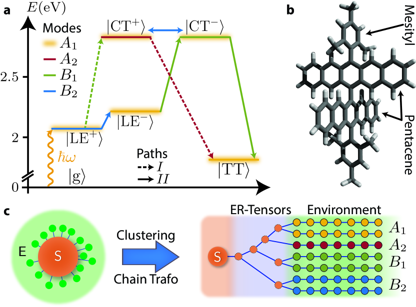
Figure 1: Reaction pathways and modelling. (a) Electronic states and their coupling through vibrational modes in DP-Mes (b), coloured by their symmetry within the point group $D_{2d}$. After photoexcitation of $\text{LE}^{+}$, SF can proceed via pathway I (dotted) or II (lines). (c) Once clustering identified symmetries and coupling patterns within the full vibrational environment (E), each cluster of modes is transformed onto chains to yield the model Hamiltonian. In the TTNS (right), all environmental states are connected to the electronic states (S) through a network of entanglement renormalisation (ER) tensors to improve speed and accuracy.

Ab initio TD-DFT calculations have been performed on DP-Mes to derive a microscopic Hamiltonian model, spanned by five electronic diabatic states, denoted system, directly relevant to SF at the novel ‘cruciform’ geometry of its ground state (see Fig. 1 and Supplementary Fig. 1). These states are the (anti)symmetrised local exciton states $\text{LE}^{\pm}$, the (anti)symmetrised charge-transfer states $\text{CT}^{\pm}$ and the final triplet pair TT. The $\text{LE}^{\pm}$ and $\text{CT}^{\pm}$ states are coherently delocalised over the two monomer units, leading to an optically bright $\text{LE}^{+}$ and dark $\text{LE}^{-}$ state (J-dimer). We find excited state energies of $2.07\,\mathrm{eV}$ ($\text{LE}^{+}$), $2.20\,\mathrm{eV}$ ($\text{LE}^{-}$), $2.75\,\mathrm{eV}$ ($\text{CT}^{\pm}$) and $1.83\,\mathrm{eV}$ (TT), which define the diagonal of the system Hamiltonian $\bm{H}_{S}$. This makes for an ideal system for studying the role of vibronic quantum dynamics in SF, as, crucially, the molecular symmetry of the ground state geometry suppresses all electronic coupling between excited states. Thus, although SF is strongly exergonic in this dimer it is strictly forbidden unless this symmetry is broken by vibrational motion (see Supplementary Fig. 2). However, as in many SF systems, even symmetry breaking cannot induce direct coupling between $\text{LE}^{+}$ and TT. Instead, this is indirectly mediated by the high-lying CT states via super-exchange Smith and Michl (2013); Berkelbach et al. (2013a, b), which is why they must be included in both the ab initio and dynamical simulations, even if they are never populated Berkelbach et al. (2013a).

We then employ further DFT calculations to construct a linear vibronic HamiltonianKuppel et al. (1984)

$$\hat{\bm{H}}_{LVC}=\bm{H}_{S}+\sum_{n=1}^{252}\bm{W}_{n}\frac{(\hat{b}^{\dagger}_{n}+\hat{b}_{n})}{\sqrt{2}}+\hat{H}_{vib},$$ (1)

based on $252$ quantum harmonic normal modes $\hat{b}_{n}^{\dagger}$ of the dimer’s ground state potential. This describes the emerging electronic couplings $\bm{W}_{n}$ as the system is perturbed from the ground state geometry (see Supplementary Sec. II).

Interface to TTNS. Following previous t-DMRG and Matrix Product State (MPS) approaches, we then perform a unitary transformation to cast $\hat{H}_{vib}$ into an equivalent system of independent 1D-chain environments (Fig.1c). The orthogonal polynomial chain transformationChin et al. (2010); Prior et al. (2010); Schröder and Chin (2016) directly exposes the low entanglement properties of the environments, which are essential for its efficient simulation with tensor wave functions (vide infra). However, the transformation can only be applied to modes with identical coupling pattern $\overline{\bm{W}}_{n}$ and arbitrary strengths $\lambda_{n}$, where $\bm{W}_{n}=\lambda_{n}\overline{\bm{W}}_{n}$. While this is often the case in toy models (allowing the entire environment to be lumped into a single chain), our ab initio patterns $\overline{\bm{W}}_{n}$ show $n$-dependent variations that grow with the irregularity and size of the molecular structure. In order to group modes with similar $\overline{\bm{W}}_{n}$, we employ unsupervised machine learning in the form of k-means clusteringArthur and Vassilvitskii (2007). Thereby, we can find the minimal required set of environments $i$ and their coupling operators $\overline{\bm{W}}_{i}$ that optimally approximate $\overline{\bm{W}}_{n}$ of assigned modes. We find that DP-Mes couplings require a minimum of four clusters, as confirmed by group theory, one for each 1D irreducible representation (irreps) $A_{1/2}$ and $B_{1/2}$ of the approximate point group $D_{2d}$ of DP-Mes. However, the large variances of the couplings are only sufficiently described by seven clusters (see Supplementary Fig. 3).

The transformation of each cluster into chains $\hat{H}_{c,i}$ yields the star-like Hamiltonian (see Fig. 1c)

$$\hat{\bm{H}}_{star}=\bm{H}_{S}+\sum_{i=1}^{7}\left[\overline{\bm{W}}_{i}\left\lVert\bm{\lambda}_{i}\right\rVert\frac{(\hat{a}^{\dagger}_{i,0}+\hat{a}_{i,0})}{\sqrt{2}}+\hat{H}_{c,i}\right],$$ (2)

where $\bm{\lambda}_{i}=(\lambda_{i_{1}},\ldots,\lambda_{i_{n}})$, and $a_{i,0}^{\dagger}$ is termed the reaction coordinate (RC) of chain $i$, which directly reflects collective motion and time scales of the bath. The matrices $\overline{\bm{W}}_{i}$ and parameters of our model are given in the Supplementary Sec. II.

TTNS for vibronic quantum dynamics. The model is simulated with tree tensor network states (TTNS) Shi et al. (2006); Szalay et al. (2015), which extend matrix-product state (MPS) methods for open quantum systemsSchollwöck (2011); Verstraete et al. (2004); Prior et al. (2010); Guo et al. (2012); Orús (2014); Schröder and Chin (2016); Wall et al. (2016) to models with multiple bosonic environments.

The strength of this method lies in an optimal approximate compression of the full vibronic system-environment wave function. It relies on the fact that the vast majority of the formally exponentially large Hilbert space is never explored, allowing a low-rank tensor approximation scheme that decomposes the wave function to yield a connected network of small, individually updatable tensors that enable controllable approximation and efficient storage and manipulation of the full quantum state (see Supplementary Sec. III and references within for formal details).

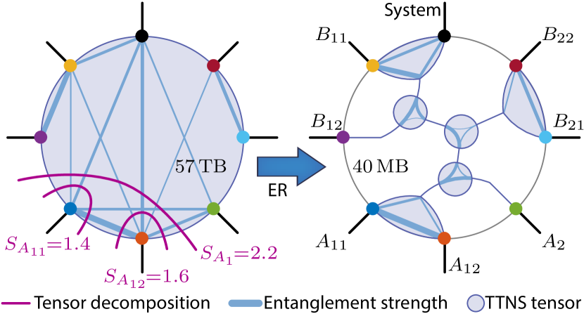
Figure 2: Entanglement renormalisation for tensor compression. The 8th order tensor (left) is compressed from $57\,\mathrm{TB}$ down to $40\,\mathrm{MB}$ by replacement with a network of 3rd order ER-tensors (right). This network is designed to optimally encode the entanglement between all environments. Discrepancies in entropy $S$ between multiple tensor decompositions (purple) reveal the tensor’s entanglement structure (blue) and guide the ER-network design.

Diagrammatically, the tensors (arrays) of a TTNS are represented as shapes with one open bond (line) per array dimension. The multiplication of two tensors is drawn as a joining of the respective bonds (see Fig. 2). A key figure regarding memory requirements is the bond dimension $D$, the size of the array dimensions and equal to the number of ‘auxiliary’ states that encode the quantum correlations between neighbouring degrees of freedom Schollwöck (2011); Orús (2014); Vidal (2007). $D$ thus governs the amount of entanglement that can be simulated, as measured by the von Neumann entropy $S=-\mathrm{Tr}(\rho\ln\rho)$, and typically ranges within $D\in[10,100]$ for acceptable results. A single TTNS tensor scales exponentially $\mathcal{O}(D^{N})$ in the number of nearest neighbours. The chain tensors are relatively ‘cheap’ to simulate (N=2), which is the essential motivation for the chain transformation. However, the central tensor, representing the electronic system and connecting to each bath suffers a curse of dimensionality. Although clustering and chain transformations reduced its $N$-neighbours from 252 in $\hat{\bm{H}}_{LVC}$ down to 7 in $\hat{\bm{H}}_{star}$, the central tensor still requires $57\,\mathrm{TB}$ of memory.

Remarkably, we can compress the tensor down to $40\,\mathrm{MB}$ by decomposing it into a loop-free tree network of smaller auxiliary entanglement renormalisation (ER) tensorsVidal (2007); Evenbly and Vidal (2009)(Fig. 2). Their connectivity optimally exploits inter-environment entanglement (blue) to minimise the entropy $S$ across all bonds, which maximises the achievable accuracy at fixed $D$. This ER-tree reduces complexity to $\mathcal{O}(ND^{3})$ and is a key enabler for applying TTNS to $N>3$ environment models.

Our TTNS is time-evolved with the time-dependent variational principle (TDVP)Haegeman et al. (2016); Lubich et al. (2015); Lubich (2015); Schröder and Chin (2016), that has proven to be faster than competing algorithmsZwolak and Vidal (2004); Schröder and Chin (2016), and establishes intriguing links to MCTDHF Lubich (2015). In this scheme, each tensor is sequentially time-evolved with a local effective Hamiltonian $\bm{H}^{eff}(t)$ that is constructed at each time step from the full many-body state, allowing long-ranged interactions, which is crucial for building and updating the ER-network. All simulations are performed at zero temperature, with no environmental excitations, and start initially from the optically bright $\text{LE}^{+}$.

Fission dynamics in DP-Mes.

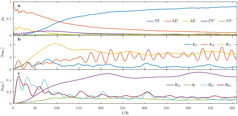
Figure 3: Simulated SF dynamics in DP-Mes. Electronic populations (a) and environmental RC occupation dynamics (b,c). For $<20\,\mathrm{fs}$ damped Rabi oscillations transfer population from $\text{LE}^{+}$ to $\text{LE}^{-}$ and $\text{CT}^{+}$. At subsequent times TT mirrors the $\text{LE}^{+}$ decay leading to SF on a timescale of $200\,\mathrm{fs}$ and suggesting a direct SF pathway. Similar timescales are present in the bath excitation $\braket{n_{RC}}$ of $B_{1}$ and $B_{2}$. The final TT yield reaches $90\%$ after $1\,\mathrm{ps}$.

Figure 3 presents numerically exact electronic population dynamics (a) and the environmental occupation of the RCs across different orders of magnitude (b,c). Vibrationally mediated SF happens on a timescale of $200\,\mathrm{fs}$ (Fig. 3c), with a final TT yield of $\approx 90\%$, comparable to experiments where yields around $94\%$ and timescales of $400-700\,\mathrm{fs}$ have been reportedLukman et al. (2015). Considering the typical instrument response of $100\,\mathrm{fs}$ and the limitations of TD-DFT in vacuum, while experiments were performed in solutions, this result appears entirely reasonable. The dynamics are multiscale; at early times $<20\,\mathrm{fs}$ they are dominated by ultrafast damped vacuum Rabi oscillations ($\text{LE}^{+}\xleftrightarrow{B_{1}}\text{CT}^{+},\text{LE}^{+}\xleftrightarrow{B_{2}}\text{LE}^{-}$, see Fig. 3a), with significant population transfer between $\text{LE}^{+}$ and $\text{LE}^{-}$ accompanied by rapid oscillatory excitation of the RCs of the $B_{2}$ environments coupling these states (see Supplementary Fig. 10). The Rabi oscillations of $\text{CT}^{+}$ correlate with the initial increase of TT population $d\rho_{\text{TT}}/dt$ indicating a small contribution of path I through $A_{2}$ (Fig. 4). This oscillatory exchange of quanta results from nuclear motion that allows us to resolve the initial mixing of $\text{LE}^{\pm}$ and $\text{CT}^{\pm}$ which allows super-exchange to occur Beljonne et al. (2013); Bakulin et al. (2015). Following this mixing ($>50\,\mathrm{fs}$), the population of the TT state quickly begins to rise, mirroring the decay of the $\text{LE}^{+}$ state, and accompanied by strong excitation of the $B_{1}$ RCs. These vibrations couple both $\text{LE}^{-}$ and TT via $\text{CT}^{-}$, and thus open the vibronic super-exchange channel, labelled path II in Fig. 1. The appearance of a strong imaginary coherence Im($\rho_{\text{TT},\text{LE}^{-}}$) indicates coherent transport between respective states, which is only possible because the common environment ($B_{1}$) mediates the coupling. Since it also matches the major increase in TT population $d\rho_{\text{TT}}/dt$, it is a strong evidence that the $B_{1}$ super-exchange drives SF (see Fig. 4). The final $5\%$ $\text{CT}^{-}$ content also shows that we reach a bound TT state which is lower in energy than a T+T (or non-relaxed TT state)Kolomeisky et al. (2014); Stern et al. (2017); Yong et al. (2017). The non-vanishing $\text{LE}^{\pm}$ on the other hand indicates that the equilibrium state can exhibit singlet character in its excited state absorption Lukman et al. (2015), We also note that the TT population is modulated by the fast $A_{1,2}$ tuning modes which could be observable in ultrafast vibrational spectroscopy Musser et al. (2015). Finally, although the model is purely harmonic, the vibrational motion we see is effectively damped. This dissipation originates from anharmonicity induced by the tuning modes coupled to the electronic states, leading to energy transfer between coupling modes which can only occur through the presence and interaction of multiple independent environments. Given the different roles of each environment in this system, an interesting idea to explore would be whether inter-environment energy transfer could be further harnessed to control/coordinate optoelectronic processes.

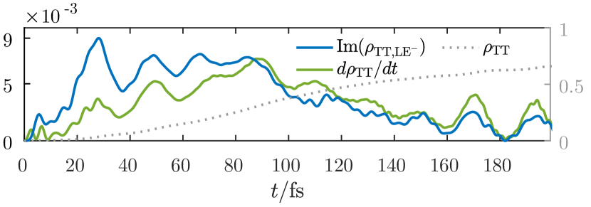
Figure 4: Evidence for coherent transport. The change $d\rho_{\text{TT}}/dt$ of $\rho_{\text{TT}}$ correlates with the dynamic coherence Im($\rho_{\text{TT},\text{LE}^{-}}$) indicating coherent super-exchange via $B_{1}$. The large oscillations with period of $20\,\mathrm{fs}$ correlate with $A_{1,2}$ oscillations (see Fig. 3b). The maximum SF rate is achieved at $90\,\mathrm{fs}$ during the passage of the avoided crossing in the TES.

Dynamic energy surfaces.

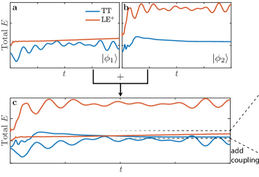
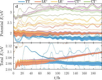
Figure 5: Energy surfaces and their electronic populations. Each bath state $\ket{\phi_{i}}$ creates its own set of five energy surfaces (a,b,simplified). Combining them for five different $\ket{\phi_{i}}$, as sketched in (c), generates the presented 25 energy surfaces (d,e). The filled areas indicate the amount of electronic population on each surface. The surfaces (dots) are coloured according to their mixing of electronic states. (d) The SF dynamics are not caused by conical intersections in the adiabatic PES. (e) Instead the vibronic mixing and super-exchange is sufficient to produce an avoided crossing at $80\,\mathrm{fs}$ of $\text{LE}^{+}$ and TT in the non-adiabatic TES causing rapid SF.

In the following, we calculate adiabatic potential energy surfaces (PES) and total energy surfaces (TES), which also include the non-adiabatic nuclear kinetic energy operator to gain a deeper understanding of the mechanism behind SF in DP-Mes. A major difficulty of visualising energy surfaces for $N>2$ vibrational modes is that the coordinate $\bm{x}=(x_{1},\ldots,x_{N})$ is multi-dimensional. Usually, this problem is overcome by presenting the potentials along two selected modes which are considered relevant reaction coordinates. We avoid this limitation by plotting the surfaces against time $t$, to obtain reaction energy profiles. These follow the optimal paths chosen by the exact wave function dynamics, unravelling them into a single dimension (see Fig. 5).

We calculate the energy surfaces on-the-fly as the eigenvalues of the effective Hamiltonian $\bm{H}^{eff}(t)$ and potential $\bm{V}^{eff}(t)$

$$H^{eff}_{(ij),(k,l)}(t) =\bra{\phi_{i}(t)}\bra{j}\hat{\bm{H}}\ket{\phi_{k}(t)}\ket{l},$$ (3)

$$V^{eff}_{(ij),(kl)}(t) =\bra{\phi_{i}(t)}\bra{j}\hat{\bm{H}}-\hat{\bm{T}}\ket{\phi_{k}(t)}\ket{l},$$ (4)

where $i,k$ index bath states and $j,l$ denote the electronic states. We simultaneously consider five different bath states $\ket{\phi_{i}(t)}$, where each $\ket{\phi_{i}(t)}$ relates to a many-body superposition of elementary, localised phonon wave packets $\ket{\varphi_{j}(\bm{x}(t))}$ (see Supplementary Sec. V) and are mutually orthogonal, i.e. $\braket{\phi_{i}(t)}{\phi_{j}(t)}=\delta_{ij}$. These states can be found at each time point from the singular value decomposition (SVD) of the total (pure) wave function for a bipartition into system and environment degrees of freedom. The SVD confirms that there are at most five environmental configurations, which generate an effective Hamiltonian $H_{eff}(t)\in\mathbb{C}^{25\times 25}$, leading to 25 surfaces (Fig. 5a-c, simplified for two states and two configurations). Indeed, the SVD is a central element in the numerical algorithm for updating and normalising the TTNS, enabling facile extraction of these configurations. Our method is basis-free, independent on the choice of local oscillator wave functions, since we use $\bm{V}^{eff}(t)$ and $\bm{H}^{eff}(t)$ only. Here, the wave function mostly populates only two surfaces (see Fig. 5d,e) which we will focus on in the following. In contrast to the population and occupation dynamics we now look into the energetics of the dynamics (Fig. 5d,e) which are revealed as changes of the energy level (dots), the overall population of each surface (fills), and even the mixing of diabatic electronic states (colour of fills) on the surfaces.

For each electronic state we can observe five energy surfaces (Fig. 5d), each caused by a different nuclear configuration $\ket{\phi_{i}(t)}$. Oscillatory features are created by normal mode displacements and can be assigned to specific environments. As an example, the dominant oscillations with $\approx 20\,\mathrm{fs}$ period visible in the highest PES of $\text{CT}^{\pm}$ are created by $A_{1,2}$ displacements tuning the energy levels (cf. Fig. 3b). Avoided crossings between energy surfaces indicate coupling between the respective diabatic states, accompanied by state mixing expressed in changing surface colour (see Fig. 5e). The SF dynamics in the adiabatic PES (Fig. 5d) are evident as population transfer from the lowest $\text{LE}^{+}$ surface to the lowest TT surface. Since the population transfers between non-crossing surfaces, this displays the non-adiabatic nature of the dynamics.

The adiabatic PES of the populated TT (blue) stays consistently below the $\text{LE}^{+}$ PES (red, Fig. 5d), thus SF in DP-Mes should not be caused by a conical intersection as proposed for other SF systemsMusser et al. (2015); Miyata et al. (2017). The crossings of the highest energy TT PES and the main $\text{LE}^{+}$ PES are not conical intersections and do not transfer populations, as they correspond to spatially separated and uncorrelated environmental states. Instead, SF is driven by an avoided crossing visible in the non-adiabatic TES (Fig. 5e) at $80\,\mathrm{fs}$, caused by three main factors. First, the unoccupied TT TES is pushed above the $\text{LE}^{+}$ TES at $20\,\mathrm{fs}$ by $A_{12}$ and $B_{22}$, as indicated by correlations with their RC displacement and excitation (see Supplementary Fig. 7). Secondly, the TT is effectively coupled to the $\text{LE}^{+}$ by super-exchange, resulting in the avoided crossing gap of $11\,\mathrm{meV}$. The third factor is the lowering of TT through the avoided crossing which leads to population transfer onto TT.

The above time scales are found in the environment’s RC frequencies, reflecting properties of the collective motion, giving us more information about the underlying mechanisms. While the energy increase of the (unoccupied) TT TES at $20\,\mathrm{fs}$ is caused by the response of the collective modes $\omega_{RC,A_{12}}\approx 1377\,\mathrm{cm^{-1}}\sim 24\,\mathrm{fs}$ and $\omega_{RC,B_{2}}\approx 1100\,\mathrm{cm^{-1}}\sim 30\,\mathrm{fs}$ to the sudden occupation of the $\text{LE}^{+}$ state, the effective vibronic coupling emerges from displacement of $B_{2}$ and $\omega_{B_{1}}\approx 400\,\mathrm{cm^{-1}}\sim 83\,\mathrm{fs}$, setting a longer time scale for SF (Fig. 3b,d). The slow reorganisation of $B_{1}$ increases the effective TT-$\text{LE}^{+}$ coupling from $3\,\mathrm{meV}$ at $20\,\mathrm{fs}$ to $6\,\mathrm{meV}$ at $80\,\mathrm{fs}$, as seen from the avoided crossing gaps. Crucially, the $B_{1}$ modes also lead to the TT TES descent, slow enough in the Landau-Zener sense to minimise the residual $\text{LE}^{+}$ population on the upper surface, in contrast to the rapid crossing at $20\,\mathrm{fs}$, where the effective coupling is weaker and no population transferred. Estimates based on the Landau-Zener formula for the diabatic transition probability predict a coupling of $10\,\mathrm{meV}$ which is encouragingly close to our result (see Supplementary Sec. VI E). This confirms that vibrationally mediated SF can be fast without the need for a conical intersection. Moreover, it suggests that SF rates and yields might be controlled by altering RC vibrational frequencies by isotopic substitutions, for example. Finally, the more direct path I via $A_{2}$ has only minor contribution to SF, since its TT projected RC occupation rapidly drops, which can only happen if TT was populated through $\text{CT}^{-}$ (see Supplementary Sec. VI D).

Conclusions. By uniquely combining a number of recent approaches to many-body simulation, we have shown how the non-perturbative dynamics of a realistically parameterised molecular dimer can be obtained and microscopically analysed by tensor network and machine learning methods. Understanding the entanglement ‘topology’ of many-body entangled states is essential for an appropriate entanglement encoding and state compression, which is at the heart of TTNS, as well as neural network stateCarleo and Troyer (2017) approaches. The crucial advance is the introduction of a flexible network topology that optimally distributes and encodes the strong entanglement between the core system and its multiple environments into numerically tractable elements. This understanding is provided by multi-environment open system models as general framework and can be transferred to more complex applications in strongly correlated electrons in quantum chemistry Szalay et al. (2015) and correlated materials design. The insights possible from exploiting TTNS-like methods are highlighted in our SF example, where we have identified the underlying mechanism, origin of timescales and, hence, the sequence of multi-environment reorganisations that drive efficient SF in a symmetry forbidden dimer. Further investigation of the real-time role of vibronic effects and dynamical symmetry breaking may suggest other ways to optimise SF, such as reducing triplet-triplet annihilation or promoting their spin-decorrelation and spatial separation. Indeed, the more general idea of designing functional molecular and condensed matter nanostructures optimised for multiscale non-equilibrium properties is an intriguing, albeit challenging idea Brédas et al. (2017); Romero et al. (2017); Scholes et al. (2017), for which powerful methods for simulating ab inito-parameterised open quantum dynamics will be essential.

Methods

DFT

All DFT calculations were performed with the NWChem electronic structure code in vacuum Valiev et al. (2010). The ground-state structure and vibrational modes were obtained employing analytical Hessians at the cc-PVDZ/B3LYP level of theory. Excited state energies and forces (corresponding to the diagonal elements of $\bm{W}$) for $\text{LE}^{\pm}$ and $\text{CT}^{\pm}$ were calculated from (linear-response) TDDFT gradients at the cc-PVDZ/LC-BLYP level of theory. The long-range corrected functional is required to correctly describe the $S_{1}$ state of pentacene as well as the states with charge-transfer character. An optimised range-separation parameter $\mu=0.29$ was used in the LC-BLYP functional. This choice gives a good description of the energy of the first excited singlet of the pentacene molecule Wong and Hsieh (2010). For TT the quintet state (total spin 2) was used as a proxy for the purpose of calculating energy and forces. The frontier molecular orbitals at the cc-PVDZ/LC-BLYP level were also used as inputs for the evaluation of the off-diagonal couplings. Modes below $110\,\mathrm{cm^{-1}}$ and above $1500\,\mathrm{cm^{-1}}$ were disregarded due to either unrealistic ab initio parameters arising from the neglect of their anharmonicities or irrelevance for present time-resolved experiments, respectively. Limitations of the method are discussed in the Supplementary Sec. I.

Tensor Network States

To prepare the linear vibronic DP-Mes Hamiltonian for the TTNS simulations, the vibrational modes were clustered to independent environments by using a weighted k-means algorithmArthur and Vassilvitskii (2007). These environments were then mapped onto chain Hamiltonians with the orthogonal polynomials transformation to facilitate the tensor tree network decomposition and numerical evolution of the complete vibronic wave function Chin et al. (2010)

The model was simulated with a TTNS as depicted in Supplementary Fig. 4, incorporating entanglement renormalisation (ER) tensors connecting the vibrational chain environments to the excitonic states and using an optimised boson basis (OBB) to allow for a large and expandable Fock basis. The time-evolution is performed in the time-dependent variational principle (TDVP)Haegeman et al. (2016) to simulate exciton-phonon dynamics at zero temperature with no initial environmental excitations at a time step of $0.33\,\mathrm{fs}$. Details about the TDVP algorithm we have developed for the TTNS evolution are given in the Supplementary Sec. II and further background can be found in Refs. Haegeman et al., 2016; Lubich et al., 2015; Szalay et al., 2015; Schröder and Chin, 2016; Shi et al., 2006. We keep 100 bosonic Fock states per vibrational mode. The dynamics converged sufficiently for an OBB dimension of 40, maximum TTNS bond dimension $D$ between ER-nodes of $D_{Node,max}=80$, while along the chains $D_{Chain,max}=30$ was appropriate (see Supplementary Fig. 5). Thus we cover a Hilbert space of $10^{500}$ states using only $10^{7}$ parameters. Energy surfaces were calculated from the effective Hamiltonian and effective potential of the system tensor. Further computational details are provided in Supplementary Sections III, IV, and V.

Data Availability

The data underlying this publication are available in the University of Cambridge data repository at URL.

Code Availability

The custom tree tensor networks state code used for simulations can be accessed at URL.

Author Contributions

F.A.Y.N.S. developed the TTNS method and performed calculations and D.H.P.T. performed DFT calculations. F.A.Y.N.S., D.H.P.T. and A.W.C. interpreted results and wrote the manuscript. A.J.M. initiated the project and provided experimental expertise. A.J.M., N.D.M.H. and A.W.C. supervised the project. All authors discussed results and contributed to the manuscript.

Competing financial interests

The authors declare no competing financial interests.

References

- Brédas et al. (2017) J.-L. Brédas, E. H. Sargent, and G. D. Scholes, Nature Materials 16, 35 (2017).
- Romero et al. (2017) E. Romero, V. I. Novoderezhkin, and R. van Grondelle, Nature 543, 355 (2017).
- Scholes et al. (2017) G. D. Scholes, G. R. Fleming, L. X. Chen, A. Aspuru-Guzik, A. Buchleitner, D. F. Coker, G. S. Engel, R. van Grondelle, A. Ishizaki, D. M. Jonas, et al., Nature 543, 647 (2017).
- Smith and Michl (2013) M. B. Smith and J. Michl, Annual Review of Physical Chemistry 64, 361 (2013).
- Berkelbach et al. (2013a) T. C. Berkelbach, M. S. Hybertsen, and D. R. Reichman, The Journal of Chemical Physics 138, 114102 (2013a).
- Shockley and Queisser (1961) W. Shockley and H. J. Queisser, Journal of Applied Physics 32, 510 (1961).
- Wilson et al. (2013) M. W. B. Wilson, A. Rao, B. Ehrler, and R. H. Friend, Accounts of Chemical Research 46, 1330 (2013).
- Walker et al. (2013) B. J. Walker, A. J. Musser, D. Beljonne, and R. H. Friend, Nature Chemistry 5, 1019 (2013).
- Yost et al. (2014) S. R. Yost, J. Lee, M. W. B. Wilson, T. Wu, D. P. McMahon, R. R. Parkhurst, N. J. Thompson, D. N. Congreve, A. Rao, K. Johnson, M. Y. Sfeir, M. G. Bawendi, T. M. Swager, R. H. Friend, M. A. Baldo, and T. Van Voorhis, Nature Chemistry 6, 492 (2014).
- Alguire et al. (2015) E. C. Alguire, J. E. Subotnik, and N. H. Damrauer, The Journal of Physical Chemistry A 119, 299 (2015).
- Tamura et al. (2015) H. Tamura, M. Huix-Rotllant, I. Burghardt, Y. Olivier, and D. Beljonne, Physical Review Letters 115, 107401 (2015), arXiv:1504.05088 .
- Zheng et al. (2016) J. Zheng, Y. Xie, S. Jiang, and Z. Lan, The Journal of Physical Chemistry C 120, 1375 (2016).
- Bakulin et al. (2015) A. A. Bakulin, S. E. Morgan, T. B. Kehoe, M. W. B. Wilson, A. W. Chin, D. Zigmantas, D. Egorova, and A. Rao, Nature Chemistry 8, 16 (2015).
- Musser et al. (2015) A. J. Musser, M. Liebel, C. Schnedermann, T. Wende, T. B. Kehoe, A. Rao, and P. Kukura, Nature Physics 11, 352 (2015).
- Fuemmeler et al. (2016) E. G. Fuemmeler, S. N. Sanders, A. B. Pun, E. Kumarasamy, T. Zeng, K. Miyata, M. L. Steigerwald, X.-Y. Zhu, M. Y. Sfeir, L. M. Campos, and N. Ananth, ACS Central Science 2, 316 (2016).
- Miyata et al. (2017) K. Miyata, Y. Kurashige, K. Watanabe, T. Sugimoto, S. Takahashi, S. Tanaka, J. Takeya, T. Yanai, and Y. Matsumoto, Nature Chemistry 9, 983 (2017).
- Stern et al. (2017) H. L. Stern, A. Cheminal, S. R. Yost, K. Broch, S. L. Bayliss, K. Chen, M. Tabachnyk, K. Thorley, N. Greenham, J. M. Hodgkiss, J. Anthony, M. Head-Gordon, A. J. Musser, A. Rao, and R. H. Friend, Nature Chemistry (2017), 10.1038/nchem.2856, arXiv:1704.01695 .
- Tempelaar and Reichman (2017) R. Tempelaar and D. R. Reichman, The Journal of Chemical Physics 146, 174703 (2017).
- Berkelbach et al. (2013b) T. C. Berkelbach, M. S. Hybertsen, and D. R. Reichman, The Journal of Chemical Physics 138, 114103 (2013b), arXiv:1211.6459v1 .
- Morrison and Herbert (2017) A. F. Morrison and J. M. Herbert, Journal of Physical Chemistry Letters 8, 1442 (2017).
- Wang and Thoss (2003) H. Wang and M. Thoss, The Journal of Chemical Physics 119, 1289 (2003).
- Worth and Cederbaum (2004) G. A. Worth and L. S. Cederbaum, Annual Review of Physical Chemistry 55, 127 (2004).
- Schollwöck (2011) U. Schollwöck, Annals of Physics 326, 96 (2011), arXiv:1008.3477 .
- Orús (2014) R. Orús, Annals of Physics 349, 117 (2014), arXiv:1306.2164 .
- Vidal (2007) G. Vidal, Physical Review Letters 99, 220405 (2007), arXiv:0912.1651 .
- Chin et al. (2010) A. W. Chin, Á. Rivas, S. F. Huelga, and M. B. Plenio, Journal of Mathematical Physics 51, 092109 (2010).
- Chin et al. (2013) A. W. Chin, J. Prior, R. Rosenbach, F. Caycedo-Soler, S. F. Huelga, and M. B. Plenio, Nature Physics 9, 113 (2013).
- Guo et al. (2012) C. Guo, A. Weichselbaum, J. von Delft, and M. Vojta, Physical Review Letters 108, 160401 (2012), arXiv:1110.6314v1 .
- Prior et al. (2010) J. Prior, A. W. Chin, S. F. Huelga, and M. B. Plenio, Physical Review Letters 105, 050404 (2010).
- Schröder and Chin (2016) F. A. Y. N. Schröder and A. W. Chin, Physical Review B 93, 075105 (2016), arXiv:1507.02202 .
- Wall et al. (2016) M. L. Wall, A. Safavi-Naini, and A. M. Rey, Physical Review A 94, 053637 (2016), arXiv:1606.08781 .
- Haegeman et al. (2016) J. Haegeman, C. Lubich, I. Oseledets, B. Vandereycken, and F. Verstraete, Physical Review B 94, 165116 (2016), arXiv:1408.5056 .
- Lukman et al. (2015) S. Lukman, A. J. Musser, K. Chen, S. Athanasopoulos, C. K. Yong, Z. Zeng, Q. Ye, C. Chi, J. M. Hodgkiss, J. Wu, R. H. Friend, and N. C. Greenham, Advanced Functional Materials 25, 5452 (2015).
- Lukman et al. (2016) S. Lukman, K. Chen, J. M. Hodgkiss, D. H. P. Turban, N. D. M. Hine, S. Dong, J. Wu, N. C. Greenham, and A. J. Musser, Nature Communications 7, 13622 (2016).
- Kuppel et al. (1984) H. Kuppel, W. Domcke, and L. S. Cederbaum, in Advances in Chemical Physics, Vol. 57, edited by I. Prigogine and S. A. Rice (John Wiley & Sons, Inc., Hoboken, NJ, USA, 1984) pp. 59–246.
- Arthur and Vassilvitskii (2007) D. Arthur and S. Vassilvitskii, in Proceedings of the Eighteenth Annual ACM-SIAM Symposium on Discrete Algorithms, SODA ’07 (Society for Industrial and Applied Mathematics, Philadelphia, PA, USA, 2007) pp. 1027–1025.
- Shi et al. (2006) Y.-Y. Shi, L.-M. Duan, and G. Vidal, Physical Review A 74, 022320 (2006), arXiv:quant-ph/0511070 .
- Szalay et al. (2015) S. Szalay, M. Pfeffer, V. Murg, G. Barcza, F. Verstraete, R. Schneider, and Ö. Legeza, International Journal of Quantum Chemistry 115, 1342 (2015), arXiv:1412.5829 .
- Verstraete et al. (2004) F. Verstraete, J. J. García-Ripoll, and J. I. Cirac, Physical Review Letters 93, 207204 (2004).
- Evenbly and Vidal (2009) G. Evenbly and G. Vidal, Physical Review B 79, 144108 (2009), arXiv:0707.1454v3 .
- Lubich et al. (2015) C. Lubich, I. V. Oseledets, and B. Vandereycken, SIAM Journal on Numerical Analysis 53, 917 (2015), arXiv:1407.2042 .
- Lubich (2015) C. Lubich, Applied Mathematics Research eXpress 2015, 311 (2015).
- Zwolak and Vidal (2004) M. Zwolak and G. Vidal, Physical Review Letters 93, 207205 (2004), arXiv:cond-mat/0406440 .
- Beljonne et al. (2013) D. Beljonne, H. Yamagata, J. L. Brédas, F. C. Spano, and Y. Olivier, Physical Review Letters 110, 226402 (2013).
- Kolomeisky et al. (2014) A. B. Kolomeisky, X. Feng, and A. I. Krylov, The Journal of Physical Chemistry C 118, 5188 (2014).
- Yong et al. (2017) C. K. Yong, A. J. Musser, S. L. Bayliss, S. Lukman, H. Tamura, O. Bubnova, R. K. Hallani, A. Meneau, R. Resel, M. Maruyama, S. Hotta, L. M. Herz, D. Beljonne, J. E. Anthony, J. Clark, and H. Sirringhaus, Nature Communications 8, 15953 (2017).
- Carleo and Troyer (2017) G. Carleo and M. Troyer, Science 355, 602 (2017), arXiv:1606.02318 .
- Valiev et al. (2010) M. Valiev, E. J. Bylaska, N. Govind, K. Kowalski, T. P. Straatsma, H. J. J. V. Dam, D. Wang, J. Nieplocha, E. Apra, T. L. Windus, and W. A. de Jong, Computer Physics Communications 181, 1477 (2010).
- Wong and Hsieh (2010) B. M. Wong and T. H. Hsieh, Journal of Chemical Theory and Computation 6, 3704 (2010).
Acknowledgements.
We thank R.H. Friend for making this work possible. F.A.Y.N.S., D.H.P.T., N.D.M.H., and A.W.C. gratefully acknowledge the support of the Winton Programme for the Physics of Sustainability and the Engineering and Physical Sciences Research Council (EPSRC).Author Contributions