Computing eigenfunctions and eigenvalues of boundary value problems with the orthogonal spectral renormalization method

Abstract

The spectral renormalization method was introduced in 2005 as an effective way to compute ground states of nonlinear Schrödinger and Gross-Pitaevskii type equations. In this paper, we introduce an orthogonal spectral renormalization (OSR) method to compute ground and excited states (and their respective eigenvalues) of linear and nonlinear eigenvalue problems. The implementation of the algorithm follows four simple steps: (i) reformulate the underlying eigenvalue problem as a fixed point equation, (ii) introduce a renormalization factor that controls the convergence properties of the iteration, (iii) perform a Gram-Schmidt orthogonalization process in order to prevent the iteration from converging to an unwanted mode; and (iv) compute the solution sought using a fixed-point iteration. The advantages of the OSR scheme over other known methods (such as Newton’s and self-consistency) are: (i) it allows the flexibility to choose large varieties of initial guesses without diverging, (ii) easy to implement especially at higher dimensions and (iii) it can easily handle problems with complex and random potentials. The OSR method is implemented on benchmark Hermitian linear and nonlinear eigenvalue problems as well as linear and nonlinear non-Hermitian $\mathcal{PT}$-symmetric models.

I Introduction

In this paper, an orthogonal spectral renormalization (OSR) method is proposed as a mean to compute ground and excited states for linear and nonlinear boundary value problems, an application which is important for quantum systems and beyond Gilboa (2018); Gilboa et al. (2016). The core idea is to recast the eigenvalue problem as a fixed point equation which is then numerically solved using a renormalized iterative scheme. The excited states are computed using a Gram-Schmidt orthogonalization process whose sole purpose is to avoid convergence to an undesired state. The proposed algorithm is robust and easy to implement particularly on problems where traditional methods (such as Newton’s and self-consistency, see e.g. Pang (2006)) are either difficult to use or fail to converge. The advantages of the OSR scheme over other well established methods are: (i) it allows the flexibility to choose large varieties of initial guesses without diverging, (ii) easy to implement especially at higher dimensions and (iii) it can easily handle problems with complex and random potentials. The OSR method is implemented on typical Hermitian linear and nonlinear eigenvalue problems. Examples include the linear harmonic and anharmonic oscillators, one-dimensional particle in a box and the nonlinear Schrödinger/Gross-Pitaevskii equation in the presence of a Hermitian harmonic trap. In addition, the OSR scheme is used to compute the spectrum of the $\mathcal{PT}$-symmetric Hamiltonian introduced originally by Bender and Boettcher Bender and Boettcher (1998) and a BEC in a double-well potential with gain and loss. The latter is modeled by the Gross-Pitaevskii equation in the presence of a complex external potential.

The applicability of the method to non-Hermitian problems is of special importance since in the last decade there has been an increased interest in non-Hermitian quantum and optical systems, especially those that obey the so-called $\mathcal{PT}$ symmetry Bender and Boettcher (1998). Generally speaking, such systems can be described by a linear Schrödinger or Gross-Pitaevskii type equation with the presence of an external complex potential $V(x)$. Space-time reflection ($\mathcal{PT}$) symmetry implies the relation $V(x)=\bar{V}(-x)$, where bar stands for complex conjugation. The physical consequences of such symmetry have been intensively studied in many branches of the physical sciences. Extensive studies exist in theoretical physics, where they cover fundamental questions in quantum mechanics Bender et al. (1999); Znojil (1999); Mehri-Dehnavi et al. (2010); Jones and Moreira (2010) and new forms of quantum field theories Bender et al. (2012); Mannheim (2013). Recently, relations of $\mathcal{PT}$ symmetry with topologically nontrivial phases in many-body systems became important Hu and Hughes (2011); Esaki et al. (2011); Ghosh (2012); Schomerus (2013); Zeuner et al. (2015); Yuce (2015); Zhu et al. (2014); Wang et al. (2015); Klett et al. (2017); Weimann et al. (2017). Since a promising approach of realizing a genuine $\mathcal{PT}$-symmetric quantum system are Bose-Einstein condensates, where atoms are removed from and added to the condensed phase Klaiman et al. (2008); Dast et al. (2013); Single et al. (2014); Gutöhrlein et al. (2015); Kreibich et al. (2016), the study of $\mathcal{PT}$ symmetry became also important within the nonlinear Gross-Pitaevskii equation. This has been done up to now in a broad variety of ways ranging from a two-mode approximation Graefe et al. (2008); Graefe (2012) to detailed descriptions in position space Dast et al. (2013); Gutöhrlein et al. (2015); Abt et al. (2015); Musslimani et al. (2008a); Schwarz et al. (2017).

Since in many special cases a formal equivalence exists between the Schrödinger equation and Maxwell’s equations, the concept of $\mathcal{PT}$ symmetry can also be studied in electromagnetic waves such as microwave cavities Bittner et al. (2012) or even in electronic devices Schindler et al. (2011). The most dramatic advances have been achieved in optics, where the notion of $\mathcal{PT}$ symmetry can be used to describe wave guides with complex refractive indices Klaiman et al. (2008); Makris et al. (2008); Musslimani et al. (2008b); El-Ganainy et al. (2007); Schnabel et al. (2017), in which the first experimental confirmation of $\mathcal{PT}$ symmetry and $\mathcal{PT}$ symmetry breaking were made possible Guo et al. (2009); Rüter et al. (2010); Peng et al. (2014)

A central issue that frequently arises in the study of non-Hermitian (and other) systems is the calculation of ground and excited states together with their respective eigenenergies. Traditional methods such as shooting, Newton and self-consistency schemes can be (in certain cases) cumbersome to implement. In the presence of complex potentials some methods are even ruled out as, e.g., imaginary time propagations because the imaginary contributions add an oscillatory term to the exponent and the algorithm does not converge. Reliable finite element methods are possible but require initial guesses of high quality Haag et al. (2015). An effective and easy to implement alternative is to use the so-called spectral renormalization method Ablowitz et al. (2006); Ablowitz and Musslimani (2005, 2003), which was successfully used on various problems including nonlocal integrable and time-dependent systems Ablowitz and Musslimani (2013, 2017); Cole and Musslimani (2017).

The paper is organized as follows. In Sec. II we present a detailed account of what we refer to as orthogonal spectral renormalization method. In sections II.1, II.2, and II.3 the OSR method is explicitly constructed to compute the ground, first, second, and generic excited states. Modifications and simplifications valuable for practical applications are presented in Sec. III. To demonstrate the applicability of the method we study some relevant linear and nonlinear Schrödinger type operators, for which a high number of states is calculated in Sec. IV. Conclusions are drawn in Sec. V.

II Orthogonal spectral renormalization

We begin our discussion by considering a general eigenvalue problem in the form

$$L\psi+f(\psi)=E\psi\;,$$ (1)

where $L$ is a linear differential operator and $f(\psi)$ is some nonlinear function of the real or complex function $\psi.$ The problem considered here is posed on the spatial domain $\Omega$ which is either bounded, the whole real line, or the entire space for multi-dimensional problems. Equation (1) is supplemented with periodic or vanishing boundary conditions. Furthermore, it is assumed that the eigenvalue problem (1) admits a ground state and $N$ excited states which we respectively denote by $\psi_{g},\psi_{1},\cdots,\psi_{N}.$ Thus we have

$$L\psi_{j}+f(\psi_{j})=E_{j}\psi_{j}\;,\;\;\;\;\;j=g,1,2,\cdots,N\;.$$ (2)

Note that in the presence of a nonlinear term, there are of course many different notions of eigenvalue problems associated with Eq. (2). Since we are interested in quantum mechanical systems, it is in addition assumed that all eigenfunctions $\psi_{j}$ are square integrable and satisfy the normalization condition

$$\int_{\Omega}dx|\psi_{j}|^{2}=1\;,\;\;\;\;\;j=g,1,2,\cdots,N\;.$$ (3)

Importantly, it is further assumed that all eigenfunctions are mutually orthogonal with respect to some type of inner product that accompany the eigenvalue problem (1). Thus, this orthogonality condition is abstractly given by

$$\langle\psi_{j},\psi_{\ell}\rangle=0\;,\;\;\;j,\ell=g,1,2,\cdots,N;\;\;\;j\neq\ell\;.$$ (4)

It should be pointed out that Sturm-Liouville theory for self-adjoint (Hermitian) linear eigenvalue problems guarantees the existence of a set of mutually orthogonal eigenstates. However, this is not the case for a linear non-Hermitian as well as for nonlinear (Hermitian or not) boundary value problems. This explains the need for the orthogonality condition (4).

In this paper, our main interest is the numerical computation of the ground and excited states $\psi_{j}$ and their respective eigenvalues (energies) $E_{j},j=g,1,2,\cdots,N$. There are several well established numerical methods that one can use to accomplish that goal. This includes Newton’s, shooting, marching and self-consistency methods to name a few Pang (2006). In 2005 the spectral renormalization (SR) scheme was proposed to compute (ground) bound states for nonlinear systems Ablowitz et al. (2006); Ablowitz and Musslimani (2005, 2003). However, when one attempts to use this method to numerically find higher-order modes it usually fails. Here, we propose an alternative SR scheme that enables one to compute excited states and their respective eigenvalues. The core idea is to implement the traditional SR algorithm interfaced with a Gram-Schmidt type orthogonalization procedure that prevents the scheme from converging to an undesired mode. We term this method orthogonal spectral renormalization. In what follows we outline the major steps in implementing this idea.

We introduce an unknown sequence of renormalization parameters $r_{j}$ (different from zero) and their respective renormalized wave functions $\varphi_{j}$ via the change of variables

$$\psi_{j}(x)=r_{j}\varphi_{j}(x)\;,\;\;\;\;\;j=g,1,2,\cdots,N\;.$$ (5)

From (3) it follows that the renormalization factors $r_{j}$ satisfy the relation

$$|r_{j}|^{2}=\frac{1}{\int_{\Omega}dx|\varphi_{j}(x)|^{2}}\;,\;\;\;\;\;j=g,1,2,\cdots,N\;.$$ (6)

The renormalized wave functions $\varphi_{j}$ satisfy the following boundary value problem induced from Eq. (1)

$$L\varphi_{j}+\frac{1}{r_{j}}f(r_{j}\varphi_{j})=E_{j}\varphi_{j}\;,\;\;\;\;\;j=g,1,2,\cdots,N\;.$$ (7)

With this at hand we next turn our focus to the question of how to devise an algorithm to approximate the renormalized eigenfunctions $\varphi_{j}$, their corresponding eigenvalues $E_{j}$ and normalizations $r_{j}$. We shall denote by $\langle u,v\rangle$ the inner product defined for any two complex-valued square integrable functions $u$ and $v$ defined by

$$\langle u,v\rangle=\int_{\Omega}u(x)\bar{v}(x)dx\;.$$ (8)

Definition (8) is usually adopted when dealing with self-adjoint eigenvalue problems. As we shall see in Sec. III.3, a different type of inner product is used for non-Hermitian systems. As mentioned above, bar denotes complex conjugation. The induced norm is given by $||u||^{2}=\langle u,u\rangle$. Taking the inner product of Eq. (7) with $\varphi_{j}$ gives an expression for the eigenvalues $E_{j}$ for all $j=g,1,2,\cdots,N$,

$$E_{j}=\frac{\langle\varphi_{j},L\varphi_{j}\rangle}{||\varphi_{j}||^{2}}+\frac{1}{r_{j}||\varphi_{j}||^{2}}\langle\varphi_{j},f(r_{j}\varphi_{j})\rangle\;.$$ (9)

We remark that solutions to Eq. (1) can be obtained using calculus of variation. Indeed, the problem can be formulated as finding the ground state that minimizes a suitable functional subject to the constraint $||\psi_{g}||=1.$ Similarly, the excited state is found by minimizing the same functional subject to the constraint in the orthogonal complement of the lower states.

Next, we proceed with the task of computing the ground, first, and $N$th excited state. The first step is to outline the computation of the ground state – which is necessary to obtain excited states.

II.1 Ground state

The renormalized ground state $\varphi_{g}$ satisfies the following eigenvalue problem which is obtained from Eq. (7)

$$L\varphi_{g}+\frac{1}{r_{g}}f(r_{g}\varphi_{g})=E_{g}\varphi_{g}\;.$$ (10)

The ground state is numerically found from the fixed point iteration

$$\varphi^{(n+1)}_{g}=\frac{1}{r^{(n)}_{g}}\left(L-E^{(n)}_{g}\right)^{-1}f\left(r^{(n)}_{g}\varphi^{(n)}_{g}\right)\;,$$ (11)

where $n=1,2,\cdots$. The ground state eigenvalue $E_{g}$ is given by

$$E^{(n)}_{g}=\frac{\langle\varphi^{(n)}_{g},L\varphi^{(n)}_{g}\rangle}{||\varphi^{(n)}_{g}||^{2}}+\frac{1}{r^{(n)}_{g}||\varphi^{(n)}_{g}||^{2}}\langle\varphi^{(n)}_{g},f(r^{(n)}_{j}\varphi^{(n)}_{g})\rangle\;,$$ (12)

with

$$|r^{(n)}_{g}|^{2}\equiv\frac{1}{||\varphi^{(n)}_{g}||^{2}}\;.$$ (13)

Upon convergence, the ground state solution for Eq. (2) is given by

$$\psi_{g}=r^{(\infty)}_{g}\varphi^{(\infty)}_{g}\;.$$ (14)

Next, we explain how to use this information to calculate the first excited state.

II.2 First excited state

The first renormalized excited state $\varphi_{1}$ satisfies the boundary value problem

$$L\varphi_{1}+\frac{1}{r_{1}}f(r_{1}\varphi_{1})=E_{1}\varphi_{1}\;.$$ (15)

If one implements the algorithm outlined in Sec. II.1, the result of the iterative process would be the ground state. To force the iteration to “go away” from the ground state we introduce a new renormalized excited state $\eta_{1}$ defined by

$$\varphi_{1}=\eta_{1}-c_{g}\psi_{g}\;,$$ (16)

where the “constant” $c_{g}$ is given by

$$c_{g}\equiv\frac{\langle\psi_{g},\eta_{1}\rangle}{||\psi_{g}||^{2}}\;.$$ (17)

Notice that this choice of the parameter $c_{g}$ would force the first excited state to be orthogonal (with respect to the inner product given in (8)) to the ground state. Indeed, we have

$$\langle\psi_{g},\varphi_{1}\rangle=0\;.$$ (18)

Since $\psi_{1}=r_{1}\varphi_{1},$ it follows that the ground and first excited states of the system are orthogonal as well. The auxiliary function $\eta_{1}$ satisfies the eigenvalue problem

$$L\eta_{1}+\frac{1}{r_{1}}f(r_{1}\varphi_{1})-E_{1}\eta_{1}=c_{g}(L-E_{1})\psi_{g}\;.$$ (19)

As a functional of the new renormalized wave function $\eta_{1},$ the first excited state eigenvalue is given by (see Eq. (15))

$$E_{1}=\frac{\langle\varphi_{1},L\varphi_{1}\rangle}{||\varphi_{1}||^{2}}+\frac{1}{r_{1}||\varphi_{1}||^{2}}\langle\varphi_{1},f(r_{1}\varphi_{1})\rangle\;,$$ (20)

where

$$|r_{1}|^{2}=\frac{1}{\int_{\Omega}dx|\eta_{1}-c_{g}\psi_{g}|^{2}}\;.$$ (21)

Equations (19) – (21) are then numerically solved with the aid of the following fixed point iteration

$$c^{(n)}_{g}\equiv\frac{\langle\psi_{g},\eta^{(n)}_{1}\rangle}{||\psi_{g}||^{2}}\;,$$ (22)

$$\varphi^{(n)}_{1}=\eta^{(n)}_{1}-c^{(n)}_{g}\psi_{g}\;,$$ (23)

$$|r^{(n)}_{1}|^{2}=\frac{1}{\int_{\Omega}dx|\eta^{(n)}_{1}-c^{(n)}_{g}\psi_{g}|^{2}}\;,$$ (24)

$$E^{(n)}_{1}=\frac{\langle\varphi^{(n)}_{1},L\varphi^{(n)}_{1}\rangle}{||\varphi^{(n)}_{1}||^{2}}+\frac{1}{r^{(n)}_{1}||\varphi^{(n)}_{1}||^{2}}\langle\varphi^{(n)}_{1},f(r^{(n)}_{1}\varphi^{(n)}_{1})\rangle\;,$$ (25)

$$\eta^{(n+1)}_{1}=-\frac{1}{r^{(n)}_{1}}(L-E^{(n)}_{1})^{-1}f(r_{1}\varphi^{(n)}_{1})+c^{(n)}_{g}\psi_{g}\;.$$ (26)

Thus, the implementation of the orthogonal spectral renormalization algorithm goes as follows: We first give an initial guess $\eta^{(1)}_{1}(x)$ and compute the “constant” $c_{g}^{(1)}$ from Eq. (22). From Eq. (23) we have $\varphi^{(1)}_{1}$ which is then used in Eqs. (24) and (25) to obtain approximations for the renormalization constant $r_{1}^{(1)}$ and eigenvalue $E_{1}^{(1)}.$ The renormalized eigenfunction $\eta_{1}^{(1)}$ is then updated using Eq. (26).

II.3 $N$th excited state

The computation of an arbitrary excited state can be constructed from knowledge of the ground and previous higher-order modes. By denoting $\varphi_{N},$ the $N^{{\rm th}}$ renormalized excited state, we have

$$L\varphi_{N}+\frac{1}{r_{N}}f(r_{N}\varphi_{N})=E_{N}\varphi_{N}\;.$$ (27)

Following the Gram-Schmidt orthogonalization process, we define a new renormalized excited state $\eta_{N}$ by

$$\varphi_{N}=\eta_{N}-\sum_{j=g}^{N-1}c_{j}\psi_{j}\;,$$ (28)

with

$$c_{j}\equiv\frac{\langle\psi_{j},\eta_{N}\rangle}{||\psi_{j}||^{2}}\;,\;\;\;\;j=g,1,2,\cdots,N-1\;.$$ (29)

As a result, we have the orthogonality condition $\langle\varphi_{N},\psi_{\ell}\rangle=0,\;\;\ell=g,1,2,\cdots,N-1.$ It can be shown that the renormalized function $\eta_{N}$ satisfies the following boundary value problem

$$L\eta_{N}+\frac{1}{r_{N}}f(r_{N}\varphi_{N})-E_{N}\eta_{N}=\sum_{\ell=g}^{N-1}c_{\ell}(L-E_{N})\psi_{\ell}\;.$$ (30)

The eigenvalue corresponding to the $N^{{\rm th}}$ excited state is given by

$$E_{N}=\frac{\langle\varphi_{N},L\varphi_{N}\rangle}{||\varphi_{N}||^{2}}+\frac{1}{r_{N}||\varphi_{N}||^{2}}\langle\varphi_{N},f(r_{N}\varphi_{N})\rangle\;,$$ (31)

where

$$|r_{N}|^{2}=\frac{1}{\int_{\Omega}dx|\eta_{N}-\sum_{j=g}^{N-1}c_{j}\psi_{j}|^{2}}\;.$$ (32)

To obtain a numerical approximation for the $N^{{\rm th}}$ excited state we iterate the following system of equations until convergence is achieved (here, $n=1,2,3,\cdots$)

$$c^{(n)}_{j}\equiv\frac{\langle\psi_{j},\eta^{(n)}_{N}\rangle}{||\psi_{j}||^{2}}\;,\;\;\;\;j=g,1,2,\cdots,N-1\;,$$ (33)

$$|r^{(n)}_{N}|^{2}=\frac{1}{\int_{\Omega}dx|\eta^{(n)}_{N}-\sum_{j=g}^{N-1}c^{(n)}_{j}\psi_{j}|^{2}}\;,$$ (34)

$$\varphi^{(n)}_{N}=\eta^{(n)}_{N}-\sum_{j=g}^{N-1}c^{(n)}_{j}\psi_{j}\;,$$ (35)

$$E^{(n)}_{N}=\frac{\langle\varphi^{(n)}_{N},L\varphi^{(n)}_{N}\rangle}{||\varphi^{(n)}_{N}||^{2}}+\frac{1}{r^{(n)}_{N}||\varphi^{(n)}_{N}||^{2}}\langle\varphi^{(n)}_{N},f(r^{(n)}_{N}\varphi^{(n)}_{N})\rangle\;,$$ (36)

$$\eta^{(n+1)}_{N}=-\frac{1}{r^{(n)}_{N}}(L-E^{(n)}_{N})^{-1}f(r^{(n)}_{N}\varphi^{(n)}_{N})+\sum_{\ell=g}^{N-1}c^{(n)}_{\ell}\psi_{\ell}\;.$$ (37)

III Numerical implementation

The basic three steps necessary for implementing the OSR method are: (i) renormalization, (ii) orthogonalization and (iii) fixed point iteration. The latter is obtained by converting the underlying linear or nonlinear boundary value problem to a fixed point (differential or integral) equation. However, as is well known, there is no unique way to reformulate a given eigenvalue problem into a fixed point equation. As such, the preferred choice is dictated by the computational efficiency and algorithm optimization.

III.1 Possible simplifications for nonlinear problems

As an example, for nonlinear problems with a Schrödinger type linear part we have

$$L=-\frac{\partial^{2}}{\partial x^{2}}+V(x)\;,$$ (38)

where $V(x)$ is either real or a complex valued potential. In this case the OSR scheme is based on the nonlinear equation

$$\left(-\frac{\partial^{2}}{\partial x^{2}}+V(x)\right)\eta_{N}+\frac{1}{r_{N}}f(r_{N}\varphi_{N})-E_{N}\eta_{N}\\ =\sum_{\ell=g}^{N-1}c_{\ell}(L-E_{N})\psi_{\ell}\;.$$ (39)

The iteration of this equation with the procedure presented in Eq. (37) can be costly (due to the required inversion of the differential operator) and spectral methods can be also cumbersome to implement. An alternative form to the fixed point iteration (37) would be to take the Fourier transform of Eq. (39), which results in the following new fixed point equation

$$\hat{\eta}^{(n+1)}_{N}=\frac{(E^{(n)}_{N}+\xi^{2})\hat{\varphi}^{(n)}_{N}}{k^{2}+\xi^{2}}+\sum_{\ell=g}^{N-1}c^{(n)}_{\ell}\hat{\psi}_{\ell}\\ -\frac{1}{k^{2}+\xi^{2}}F\left(V(x)\varphi^{(n)}_{N}+\frac{1}{r^{(n)}_{N}}f(r^{(n)}_{N}\varphi^{(n)}_{N})\right)\;.$$ (40)

The Fourier transform is denoted by $F$ and the functions $\hat{\eta}$, $\hat{\varphi}$, and $\hat{\psi}$ are the Fourier transforms of $\eta$, $\varphi$, and $\psi$, respectively. We have rewritten $-\partial^{2}/\partial x^{2}-E_{N}^{(n)}$ as $-\partial^{2}/\partial x^{2}+\xi^{2}-E_{N}^{(n)}-\xi^{2}$ with $\xi^{2}$ being an arbitrary positive number such that $-\partial^{2}/\partial x^{2}+\xi^{2}$ is positive definite.

In Eq. (40) it can be clearly seen that the term $\sum_{\ell=g}^{N-1}c^{(n)}_{\ell}\hat{\psi}_{\ell}$ only adds contributions to $\eta$ which are orthogonal with respect to the inner product (8). At the end we are not interested in these since we want to determine $\varphi_{N}$. Thus, one can, in practical applications, do without these terms and avoid the computation of their Fourier transforms. The simplified iteration reads

$$\hat{\Phi}^{(n+1)}_{N}=\frac{(E^{(n)}_{N}+\xi^{2})\hat{\varphi}^{(n)}_{N}}{k^{2}+\xi^{2}}\\ -\frac{1}{k^{2}+\xi^{2}}F\left(V(x)\varphi^{(n)}_{N}+\frac{1}{r^{(n)}_{N}}f(r^{(n)}_{N}\varphi^{(n)}_{N})\right)\;,$$ (41a)

$$\hat{\varphi}^{(n+1)}_{N}=\hat{\Phi}^{(n)}_{N}-\sum_{\ell=g}^{N-1}c^{(n)}_{\ell}\hat{\psi}_{\ell}\;,$$ (41b)

and $\hat{\Phi}^{(n)}_{N}$ is used instead of $\hat{\eta}^{(n)}_{N}$ in all other steps. Note that in this way we cannot obtain the auxiliary wave function $\eta$. This will affect only the wave functions $\hat{\Phi}_{N}$, however, the desired results $\varphi_{N}$ will be identical with those obtained from Eq. (40). For the numerical results reported in this paper, we used a fast Fourier transform and the Fourier fixed point iteration (41a) rather than inverting the operator $-\partial^{2}/\partial x^{2}+V(x)-E^{(n)}_{N}$.

III.2 Renormalization for linear operators

While the spectral renormalization was originally introduced for nonlinear operators Ablowitz et al. (2006); Ablowitz and Musslimani (2005, 2003) the iteration according to Eq. (41a) can also be applied to linear operators, i.e., $f(r^{(n)}_{N}\varphi^{(n)}_{N})=0$. In this case the renormalization factor $r_{N}^{(n)}$, calculated from Eq. (34), no longer appears in Eq. (41a) and it seems the renormalization is no longer necessary. However, in practical applications it is anyway necessary to renormalize such that the wave function will neither grow above all limits nor converge to vanishing norm.

Thus, for a linear problem the procedure is outlined below. Again, we use a simplified iteration based on Eqs. (41a) and (41b), i.e. $\hat{\Phi}^{(n)}_{N}$ is used instead of $\hat{\eta}^{(n)}_{N}$. First, the coefficients $c_{j}^{(N)}$ are computed according to Eq. (33), then the normalization constant $r_{N}^{(n)}$ is determined via Eq. (34), and $\varphi_{N}^{(n)}$ is calculated from Eq. (41b). After this, it is the best choice to introduce

$$\psi_{N}^{(n)}=r_{N}^{(n)}\varphi_{N}^{(n)}\;,$$ (42)

and to use the modification

$$E^{(n)}_{N}=\langle\psi^{(n)}_{N},L\psi^{(n)}_{N}\rangle\;,$$ (43)

of Eq. (36) to calculate the iterate of the energy eigenvalue $E^{(n)}_{N}$. Finally the next step in the iteration is obtained from the corresponding adaptation of Eq. (41a), viz.

$$\hat{\Phi}^{(n+1)}_{N}=\frac{(E^{(n)}_{N}+\xi^{2})\hat{\psi}^{(n)}_{N}}{k^{2}+\xi^{2}}-\frac{1}{k^{2}+\xi^{2}}F\left(V(x)\psi^{(n)}_{N}\right).$$ (44)

III.3 Inner product for non-Hermitian potentials

As a final comment, we presented the OSR scheme using the inner product given in Eq. (8) which is suitable for a self-adjoint linear operator $L$. For non-Hermitian systems, such as the $\mathcal{PT}$-symmetric one discussed in this paper, a more suitable inner product would be

$$\langle u,v\rangle=\int_{\Omega}\left(\mathcal{CPT}u(x)\right)v(x)dx\;,$$ (45)

where the $\mathcal{C}$ operator is defined in Refs. Bender et al. (2002); Bender (2005).

IV Examples

In this section we apply the OSR method to various linear and nonlinear eigenvalue problems including $\mathcal{PT}$-symmetric ones.

IV.1 Linear Hermitian systems

IV.1.1 Harmonic oscillator

The first example we consider is the one-dimensional simple quantum harmonic oscillator. The dimensionless Schrödinger equation reads

$$\left[-\frac{\partial^{2}}{\partial x^{2}}+x^{2}\right]\psi(x)=E\psi(x)\,.$$ (46)

We choose a field of view of $x\in[-6,6]$ with a resolution of $M=128$ points and a singularity prevention constant of $\xi^{2}=15$. The algorithm is quite insensitive about the initial guesses, therefore one can always choose the initial function $\varphi_{0}=\mathrm{e}^{-x^{2}}$ for all states. With this set of parameters it is possible to calculate the first 9 states up to machine precision (14 to 15 valid digits) within $N_{\mathrm{iter}}\approx 230$–$1230$ iterations. To calculate higher states up to machine precision, the resolution, the field of view and the singularity prevention constant have to be increased. For example a parameter set of $M=256,$ $x\in[-20,20]$ and $\xi^{2}=1000$ allows for a calculation of the first $100$ states up to machine precision. In this case the iteration count is $N_{\mathrm{iter}}\approx 11000$–$15000$. Exemplarily the resulting eigenfunctions $\varphi_{0}$ and $\varphi_{10}$ are shown in Fig. 1

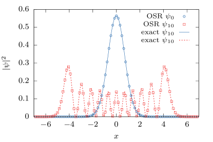
Figure 1: Eigenfunctions $\psi_{0}$ and $\psi_{10}$ of the 1d harmonic oscillator (46) calculated with the orthogonal spectral renormalization method in comparison with the exact solution.

in comparison with the analytic solution. It is remarkable that despite the rather low resolution for the highly excited states the energy matches perfectly the analytical result up to machine precision.

A calculation in two dimensions with

$$\left[-\nabla^{2}+x^{2}+y^{2}\right]\psi(x,y)=E\psi(x,y)\;,$$ (47)

shows similar results. The energy eigenvalues nicely converge to the analytically known values. Excited states can be acquired up to machine precision as well. However, if one wants to converge to the eigenstates of the quantum numbers in the Cartesian basis, i.e., $n_{x}$ and $n_{y}$, and not to some superpositions of these, even this can be achieved. In this case one has to specify the initial guesses more precisely, e.g., for the first states one can choose

$$\varphi_{00} =\mathrm{e}^{-(x^{2}+y^{2})}\,, \varphi_{10} =x\mathrm{e}^{-(x^{2}+y^{2})}\,,$$

$$\varphi_{01} =y\mathrm{e}^{-(x^{2}+y^{2})}\,, \varphi_{20} =x^{2}\mathrm{e}^{-0.5(x^{2}+y^{2})}\,,$$

$$\varphi_{11} =xy\mathrm{e}^{-(x^{2}+y^{2})}\,, \varphi_{02} =y^{2}\mathrm{e}^{-0.5(x^{2}+y^{2})}\;,$$ (48)

to obtain the required nodal structure.

IV.1.2 Anharmonic oscillator

The next example is an anharmonic quartic one-dimensional oscillator whose Schrödinger equation reads

$$\left[-\frac{\partial^{2}}{\partial x^{2}}+x^{2}+\gamma x^{4}\right]\psi(x)=E\psi(x)\,.$$ (49)

Here we choose $x\in[-8,8]$, $M=128,$ $\xi^{2}=5\cdot 10^{4}$ and $\varphi_{0}=\mathrm{e}^{-x^{2}}$. This allows for calculations up to machine precision for the first ten states up to $\gamma=10$. The spectrum in dependence of $\gamma$ for the first eight states is shown in Fig. 2

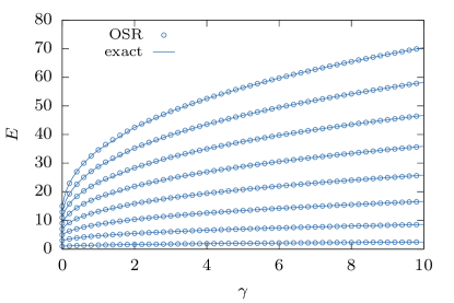
Figure 2: Spectrum of the first eight eigenstates of the anharmonic oscillator (49) calculated with the orthogonal spectral renormalization in comparison with a numerically accurate calculation from Biswas et al. (1973).

in comparison with exact calculations from Biswas et al. (1973). The agreement is perfect.

IV.1.3 Particle in a box

A third linear Hermitian example is a particle in a box with finite walls,

$$\left[-\frac{\partial^{2}}{\partial x^{2}}+V(x)\right]\psi(x)=E\psi(x)\,,$$

$$V(x)=\begin{cases}0&|x|<a\\ V_{0}&\text{otherwise}\end{cases}\,.$$ (50)

The analytical energy eigenvalues are determined by the transcendental equations

$$\sqrt{\frac{V_{0}-E}{E}} =\tan\left(\sqrt{E}a\right)\,, \text{symmetric}\,,$$ (51)

$$-\sqrt{\frac{E}{V_{0}-E}} =\tan\left(\sqrt{E}a\right)\,, \text{antisymmetric}\;.$$ (52)

We chose $a=1$ and $V_{0}=20$, which leads to three bound states with the energies

$$E_{0} =1.63948\,, E_{1} =6.44188\,, E_{2} =13.8915\,.$$ (53)

For the spectral renormalization algorithm, we choose $x\in[-5,5]$, $M=4096,$ $\xi^{2}=10$ and an initial guess of $\varphi_{0}=\mathrm{e}^{-x^{2}}$. This yields the energy eigenvalues

$$E_{0} =1.64012\,, E_{1} =6.44434\,, E_{2} =13.89634,$$ (54)

within $N_{\mathrm{iter}}\approx 60-160$ iteration steps. The corresponding wave function in comparison with the analytical solution can be found in Fig. 3.

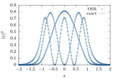
Figure 3: Eigenfunctions of the particle in the box problem (50) with $a=1$ and $V_{0}=20$. The orthogonal spectral renormalization solution is compared with the analytical solution.

For this example, the solution cannot be retrieved up to machine precision. In addition, the accuracy of the solution depends on the field of view and the resolution in a nontrivial way, therefore, a fine adjustment has to be performed to retrieve the most accurate solutions. This may result from the discontinuity at $x=a$ and the fact that the finite discretization can only approximate such a point.

IV.2 Linear $\mathcal{PT}$-symmetric systems

In this section we will demonstrate the application of the orthogonal spectral renormalization algorithm on a linear $\mathcal{PT}$-symmetric system. We use the well-known toy model of Bender and Boettcher Bender and Boettcher (1998)

$$\left[-\frac{\partial^{2}}{\partial x^{2}}-(\mathrm{i}x)^{\epsilon}\right]\psi(x)=E\psi(x)\,.$$ (55)

For the parameter $\epsilon>2$ the system possess an unbroken $\mathcal{PT}$ symmetry with an entirely real spectrum. For values $\epsilon<2$ and decreasing $\epsilon$ always two energy levels merge into a pair of complex conjugate eigenvalues. Below $\epsilon=1$ no real eigenvalues exist. The value of $\epsilon=2$ is the special case of the harmonic oscillator.

We choose the following set of parameters: $x\in[-8,8]$, $M=128,$ $\xi^{2}=2\cdot 10^{4}$ and $\varphi_{0}=\mathrm{e}^{-x^{2}}$. The resulting spectrum for the $\mathcal{PT}$-symmetric solutions can be found in Fig. 4 compared with a numerical correct solution calculated with a finite difference scheme. In the calculation for the higher excited states, the $\mathcal{CPT}$ product is used to project out the states with lower chemical potential. The algorithm works quite well to obtain the excited states. For increasing $\epsilon$ and higher states the parameter $\xi^{2}$ has to be increased as well. This explains the chosen high value of $\xi^{2}$ to converge for all selected states.

However, there is a restriction that the value $\epsilon$ cannot be increased much further than $\epsilon=3$. In addition for higher excited states the algorithm fails to converge as well, even when the renormalization factor $\xi^{2}$ is increased. This can be seen in the Fig. 4.

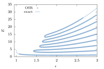
Figure 4: Spectrum of the first nine $\mathcal{PT}$-symmetric states of the complex extended harmonic oscillator model (55). The solution of the orthogonal spectral renormalization is compared with a numerically accurate solution. The algorithm fails to converge for the ground state for small $\epsilon$ close to 1 and for higher excited states for larger $\epsilon$.

For higher excited states data points are missing. The algorithm also fails to converge for the ground state for values of $\epsilon$ close to 1, in that range where the accurate ground state energy begins to diverge.

IV.3 Nonlinear Hermitian system

We now turn to nonlinear systems and study as an example the Gross-Pitaevskii equation of a Bose-Einstein condensate in a harmonic trap, viz.

$$\left[-\frac{\partial^{2}}{\partial x^{2}}+x^{2}+g|\psi|^{2}\right]\psi=E\psi\;,$$ (56)

where $g$ measures the strength of the nonlinearity and $E$ is the energy eigenvalue, which in the nonlinear problem has the physical meaning of a chemical potential.

The chemical potentials for the ground state and the first four excited states calculated with the orthogonal spectral renormalization are shown in Fig. 5

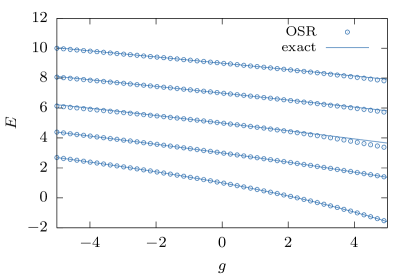
Figure 5: Spectrum of a Bose-Einstein condensate in a harmonic trap in dependence of the nonlinearity parameter $g$. The chemical potentials $E$ are calculated with the orthogonal spectral renormalization method and compared with a numerically exact calculation in an oscillator basis.

in comparison with a calculation in an oscillator basis, of which we checked that the values are numerically exact. The corresponding wave functions are shown in Fig. 6

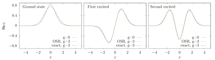
Figure 6: Wave functions of the Gross-Pitaevskii equation (56) for the ground state and the first two excited states calculated with the OSR and in an harmonic oscillator basis (exact).

and help to exemplify how the OSR works in such a nonlinear system. The initial wave function of the OSR iteration was a simple Gaussian $\varphi_{0}=\mathrm{e}^{-x^{2}}$ and we used $x\in[-7,7]$, $M=256,$ and $\xi^{2}=30$.

We can clearly observe that the ground state is found accurately. The chemical potentials of both methods match perfectly. This is also true for the first excited state. This result can be expected. As can be seen in Fig. 6 the first excited state is antisymmetric with respect to a reflection about $x=0$ whereas the ground state is symmetric. Consequently the two states are orthogonal and the calculation of the first excited state as outlined in Sec. II.2 converges nicely to the correct wave function.

For the second excited state the situation changes. The wave function is again symmetric. In the nonlinear equation there is no need for it to be orthogonal to the ground state, and in fact it is not. However, the orthogonalization scheme of the OSR will force the wave function to be orthogonal to the ground and first excited state. As a result the wave function does not converge to the desired result. Anyway for small nonlinearities the result is still a reasonable approximation, which loses in quality with increasing $g$. Since the same reason exists for all higher excited states, for all of their chemical potentials small deviations from the converged oscillator basis calculation appear for large values of $g$.

IV.4 Nonlinear non-Hermitian systems

IV.4.1 BEC in a double well with gain and loss

The next example is a one-dimensional Bose-Einstein condensate in a double-well potential with an additional complex gain-loss term. This system was introduced and discussed in Dast et al. (2013) and is described by the stationary Gross-Pitaevskii equation

$$\left[-\frac{\partial^{2}}{\partial x^{2}}+V+g|\psi|^{2}\right]\psi=E\psi\;,$$ (57)

with a complex $\mathcal{PT}$-symmetric potential given by

$$V=\omega^{2}x^{2}+V_{0}\mathrm{e}^{-\sigma x^{2}}+\mathrm{i}\Gamma x\mathrm{e}^{-\rho x^{2}}\,.$$ (58)

The parameters used in our numerical study are

$$\rho =\frac{\sigma}{2\ln\left(\frac{V_{0}\sigma}{\omega^{2}}\right)}\,, \omega =0.5\,, V_{0} =4\,, \sigma =0.5\,.$$ (59)

The real part of the potential represents the double-well trap and the imaginary part a coherent in- and outcoupling of particles in the individual wells. Here we choose the parameters $x\in[-7.5,7.5]$, $M=128$ and $\xi^{2}=30$. The system has a $\mathcal{PT}$-symmetric ground state and excited state as well as two complex conjugate $\mathcal{PT}$-broken states.

The calculated spectrum as a function of the gain-loss parameter $\Gamma$ can be found in Fig. 7

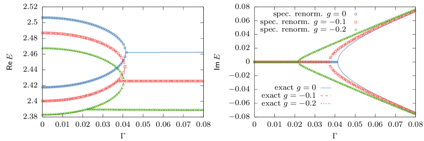
Figure 7: Spectrum of the double well (58) calculated with the orthogonal spectral renormalization method in comparison with a solution from Dast et al. (2013).

compared with the numerically accurate solution from Dast et al. (2013). In the linear case for $g=0$ the ground and excited states can be calculated perfectly. To calculate the excited state, the ground state is subtracted via the $\mathcal{CPT}$ product in each step. We use again a simple Gaussian $\varphi_{0}=\mathrm{e}^{-x^{2}}$ as initial guess. In the linear case the system becomes $\mathcal{PT}$-broken at a value of $\Gamma\approx 0.04$. For greater values there exist two complex conjugate $\mathcal{PT}$-broken states. The spectral renormalization method fails in this area to converge, independently of the initially chosen wave functions.

This changes if a nonlinearity $g\neq 0$ is introduced. Here the $\mathcal{PT}$-broken states can be calculated if one chooses a suitable initial $\mathcal{PT}$-broken guess, e.g.,

$$\varphi_{+}=1.1\mathrm{e}^{-(x-2)^{2}}+\mathrm{e}^{(x+2)^{2}}\,,$$

$$\varphi_{-}=\mathrm{e}^{-(x-2)^{2}}+1.1\mathrm{e}^{(x+2)^{2}}\,.$$ (60)

In the nonlinear system the problem arises that there is a range in which the $\mathcal{PT}$-broken states lie energetically below the $\mathcal{PT}$-symmetric ground state. In this range one can enforce a convergence into a $\mathcal{PT}$-symmetric state by dropping the imaginary part of the Fourier transformed wave function in each iteration step.

Due to the nonlinearity the states are no longer orthogonal with respect to the $\mathcal{CPT}$ product. Nevertheless, as the nonlinearity is quite small, i.e. $|g|\leq 0.2$, the states are approximately orthogonal, therefore, the acquired energy eigenvalues are correct up to the third decimal digit.

IV.4.2 2d BEC excitations with gain and loss

In a last example we consider a two-dimensional Bose-Einstein condensate trapped in a harmonic trap with optional gain-loss terms. We calculate ground and several excited states. The Gross-Pitaevskii equation reads

$$\left[-\nabla^{2}+x^{2}+y^{2}+\mathrm{i}\Gamma x\mathrm{e}^{-(x^{2}+y^{2})}+g|\psi|^{2}\right]\psi=E\psi\,.$$ (61)

This represents a harmonic trap and a $\mathcal{PT}$-symmetric gain-loss term, where $\Gamma$ is the strength of the in- and out coupling. We choose $x\in[-5,5]$, $M=128$ and $\xi^{2}=30$. Initial guesses are the harmonic oscillator ground and first excited states oriented in $x$- and $y$-direction as well as a vortex ansatz:

$$\varphi_{\mathrm{G}} =\mathrm{e}^{-(x^{2}+y^{2})}\,, \varphi_{\mathrm{V}} =(x+\mathrm{i}y)\mathrm{e}^{-(x^{2}+y^{2})}\,,$$

$$\varphi_{x} =x\mathrm{e}^{-(x^{2}+y^{2})}\,, \varphi_{y} =y\mathrm{e}^{-(x^{2}+y^{2})}\,.$$ (62)

Excited states are again calculated with the use of the $\mathcal{CPT}$ product.

The resulting spectrum as a function of the gain-loss parameter $\Gamma$ can be found in Fig. 8

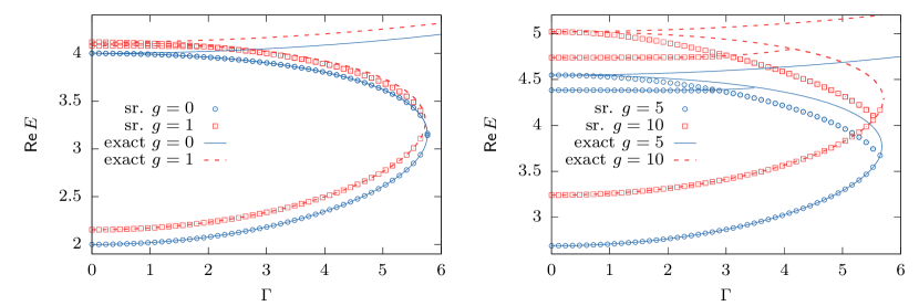
Figure 8: Spectrum of the lowest states of the two dimensional Bose-Einstein condensate in a harmonic trap with gain and loss (61). The orthogonal spectral renormalization solution is compared with a calculation in a harmonic oscillator basis Schwarz et al. (2017).

in comparison with a numerically accurate solution calculated in a harmonic oscillator basis Schwarz et al. (2017). In the linear case $g=0$ the states are perfectly orthogonal and the results match the accurate solution. In the nonlinear case with $\Gamma=0$ the states are orthogonal as well and the result is again correct. In the nonlinear non-Hermitian case the states are in general no longer orthogonal, therefore, the spectral renormalization solutions deviate the more the larger the nonlinearity $g$ is chosen. However, the state oriented in $y$-direction is orthogonal to the ground state despite the nonlinearity and non-Hermiticity, and this state can be calculated correctly, independently of the chosen value of $g$ and $\Gamma$.

V Conclusion

In this paper, we developed and presented the orthogonal spectral renormalization (OSR) method as a numerical scheme to compute ground and excited states as well as their corresponding eigenvalues, in all cases in which the states are orthogonal to each other according to a certain inner product. The scheme can be used in both linear and nonlinear boundary value problems. The OSR algorithm can be described using the following major steps: (i) rewriting the given eigenvalue problem in terms of a fixed point equation, (ii) introduce a spectral renormalization parameter whose sole purpose is to control the converge properties of the iteration, (iii) perform a Gram-Schmidt orthogonalization process that forbids the iteration from converging to an undesired (linear or nonlinear) mode; and (iv) compute the solution sought using a fixed-point iterative scheme. The proposed method extends the “classical” spectral renormalization scheme first introduced in 2005 (to compute ground state) to enable the numerical calculation of arbitrary excited states. The OSR has several advantages: (i) it allows the flexibility to choose large varieties of initial guesses without diverging, (ii) easy to code especially at higher dimensions and (iii) it can easily handle problems with complex and random potentials. The OSR method is implemented on typical Hermitian linear and nonlinear eigenvalue problems where it proved to work very fast and reliably. Examples include the linear harmonic and anharmonic oscillators, one-dimensional particle in a box and the nonlinear Schrödinger/Gross-Pitaevskii equation in the presence of a Hermitian harmonic trap. In addition, the OSR scheme is used to compute the spectrum of the $\mathcal{PT}$ symmetric Hamiltonian from the seminal work of Bender and Boettcher and a BEC in a double-well potential with gain and loss.

References

- Gilboa (2018) G. Gilboa, Nonlinear Eigenproblems in Image Processing and Computer Vision (Springer Int. Pub., 2018).
- Gilboa et al. (2016) G. Gilboa, M. Moeller, and M. Burger, J. Math. Imaging Vision 56, 300 (2016).
- Pang (2006) T. Pang, An Introduction to Computational Physics, 2nd ed. (Cambridge University Press, 2006).
- Bender and Boettcher (1998) C. M. Bender and S. Boettcher, Phys. Rev. Lett. 80, 5243 (1998).
- Bender et al. (1999) C. M. Bender, S. Boettcher, and P. N. Meisinger, J. Math. Phys. 40, 2201 (1999).
- Znojil (1999) M. Znojil, Phys. Lett. A 264, 108 (1999).
- Mehri-Dehnavi et al. (2010) H. Mehri-Dehnavi, A. Mostafazadeh, and A. Batal, J. Phys. A 43, 145301 (2010).
- Jones and Moreira (2010) H. F. Jones and E. S. Moreira, Jr, J. Phys. A 43, 055307 (2010).
- Bender et al. (2012) C. M. Bender, V. Branchina, and E. Messina, Phys. Rev. D 85, 085001 (2012).
- Mannheim (2013) P. D. Mannheim, Fortschr. Phys. 61, 140 (2013).
- Hu and Hughes (2011) Y. C. Hu and T. L. Hughes, Phys. Rev. B 84, 153101 (2011).
- Esaki et al. (2011) K. Esaki, M. Sato, K. Hasebe, and M. Kohmoto, Phys. Rev. B 84, 205128 (2011).
- Ghosh (2012) P. K. Ghosh, J. Phys.: Condens. Matter 24, 145302 (2012).
- Schomerus (2013) H. Schomerus, Opt. Lett. 38, 1912 (2013).
- Zeuner et al. (2015) J. M. Zeuner, M. C. Rechtsman, Y. Plotnik, Y. Lumer, S. Nolte, M. S. Rudner, M. Segev, and A. Szameit, Phys. Rev. Lett. 115, 040402 (2015).
- Yuce (2015) C. Yuce, Phys. Lett. A 379, 1213 (2015).
- Zhu et al. (2014) B. Zhu, R. Lü, and S. Chen, Phys. Rev. A 89, 062102 (2014).
- Wang et al. (2015) X. Wang, T. Liu, Y. Xiong, and P. Tong, Phys. Rev. A 92, 012116 (2015).
- Klett et al. (2017) M. Klett, H. Cartarius, D. Dast, J. Main, and G. Wunner, Phys. Rev. A 95, 053626 (2017).
- Weimann et al. (2017) S. Weimann, M. Kremer, Y. Plotnik, Y. Lumer, S. Nolte, K. G. Makris, M. Segev, M. C. Rechtsman, and A. Szameit, Nat. Mater. 16, 433 (2017).
- Klaiman et al. (2008) S. Klaiman, U. Günther, and N. Moiseyev, Phys. Rev. Lett. 101, 080402 (2008).
- Dast et al. (2013) D. Dast, D. Haag, H. Cartarius, G. Wunner, R. Eichler, and J. Main, Fortschr. Phys. 61, 124 (2013).
- Single et al. (2014) F. Single, H. Cartarius, G. Wunner, and J. Main, Phys. Rev. A 90, 042123 (2014).
- Gutöhrlein et al. (2015) R. Gutöhrlein, J. Schnabel, I. Iskandarov, H. Cartarius, J. Main, and G. Wunner, J. Phys. A 48, 335302 (2015).
- Kreibich et al. (2016) M. Kreibich, J. Main, H. Cartarius, and G. Wunner, Phys. Rev. A 93, 023624 (2016).
- Graefe et al. (2008) E. M. Graefe, U. Günther, H. J. Korsch, and A. E. Niederle, J. Phys. A 41, 255206 (2008).
- Graefe (2012) E. M. Graefe, J. Phys. A 45, 444015 (2012).
- Abt et al. (2015) N. Abt, H. Cartarius, and G. Wunner, Int. J. Theor. Phys. 54, 4054 (2015).
- Musslimani et al. (2008a) Z. H. Musslimani, K. G. Makris, R. El-Ganainy, and D. N. Christodoulides, J. Phys. A 41, 244019 (2008a).
- Schwarz et al. (2017) L. Schwarz, H. Cartarius, Z. H. Musslimani, J. Main, and G. Wunner, Phys. Rev. A 95, 053613 (2017).
- Bittner et al. (2012) S. Bittner, B. Dietz, U. Günther, H. L. Harney, M. Miski-Oglu, A. Richter, and F. Schäfer, Phys. Rev. Lett. 108, 024101 (2012).
- Schindler et al. (2011) J. Schindler, A. Li, M. C. Zheng, F. M. Ellis, and T. Kottos, Phys. Rev. A 84, 040101 (2011).
- Makris et al. (2008) K. G. Makris, R. El-Ganainy, D. N. Christodoulides, and Z. H. Musslimani, Phys. Rev. Lett. 100, 103904 (2008).
- Musslimani et al. (2008b) Z. H. Musslimani, K. G. Makris, R. El-Ganainy, and D. N. Christodoulides, Phys. Rev. Lett. 100, 030402 (2008b).
- El-Ganainy et al. (2007) R. El-Ganainy, K. G. Makris, D. N. Christodoulides, and Z. H. Musslimani, Opt. Lett. 32, 2632 (2007).
- Schnabel et al. (2017) J. Schnabel, H. Cartarius, J. Main, G. Wunner, and W. D. Heiss, Phys. Rev. A 95, 053868 (2017).
- Guo et al. (2009) A. Guo, G. J. Salamo, D. Duchesne, R. Morandotti, M. Volatier-Ravat, V. Aimez, G. A. Siviloglou, and D. N. Christodoulides, Phys. Rev. Lett. 103, 093902 (2009).
- Rüter et al. (2010) C. E. Rüter, K. G. Makris, R. El-Ganainy, D. N. Christodoulides, M. Segev, and D. Kip, Nat. Phys. 6, 192 (2010).
- Peng et al. (2014) B. Peng, S. K. Ozdemir, F. Lei, F. Monifi, M. Gianfreda, G. L. Long, S. Fan, F. Nori, C. M. Bender, and L. Yang, Nat. Phys. 10, 394 (2014).
- Haag et al. (2015) D. Haag, D. Dast, H. Cartarius, and G. Wunner, Int. J. Theor. Phys. 54, 4100 (2015).
- Ablowitz et al. (2006) M. J. Ablowitz, A. S. Fokas, and Z. H. Musslimani, J. Fluid Mech. 562, 313 (2006).
- Ablowitz and Musslimani (2005) M. J. Ablowitz and Z. H. Musslimani, Opt. Lett. 30, 2140 (2005).
- Ablowitz and Musslimani (2003) M. J. Ablowitz and Z. H. Musslimani, Physica D 184, 276 (2003).
- Ablowitz and Musslimani (2013) M. J. Ablowitz and Z. H. Musslimani, Phys. Rev. Lett. 110, 064105 (2013).
- Ablowitz and Musslimani (2017) M. J. Ablowitz and Z. H. Musslimani, Stud. Appl. Math. 139, 7 (2017).
- Cole and Musslimani (2017) J. T. Cole and Z. H. Musslimani, Physica D 358, 15 (2017).
- Bender et al. (2002) C. M. Bender, D. C. Brody, and H. F. Jones, Phys. Rev. Lett. 89, 270401 (2002).
- Bender (2005) C. M. Bender, Contemp. Phys. 46, 277 (2005).
- Biswas et al. (1973) S. N. Biswas, K. Datta, R. P. Saxena, P. K. Srivastava, and V. S. Varma, J. Math. Phys. 14, 1190 (1973).