Channel Estimation for TDD/FDD Massive MIMO Systems with Channel Covariance Computing

Abstract

In this paper, we propose a new channel estimation scheme for TDD/FDD massive MIMO systems by reconstructing uplink/downlink channel covariance matrices (CCMs) with the aid of array signal processing techniques. Specifically, the angle information and power angular spectrum (PAS) of each multi-path channel is extracted from the instantaneous uplink channel state information (CSI). Then, the uplink CCM is reconstructed and can be used to improve the uplink channel estimation without any additional training cost. In virtue of angle reciprocity as well as PAS reciprocity between uplink and downlink channels, the downlink CCM could also be inferred with a similar approach even for FDD massive MIMO systems. Then, the downlink instantaneous CSI can be obtained by training towards the dominant eigen-directions of each user. The proposed strategy is applicable for any kind of PAS distributions and array geometries. Numerical results are provided to demonstrate the superiority of the proposed methods over the existing ones.

I Introduction

Large-scale multiple-input multiple-output (MIMO) or “massive MIMO” is a new technique that employs hundreds or even thousands of antennas at base station (BS) to simultaneously serve multiple users and has been widely investigated for its numerous merits, such as high spectrum and energy efficiency, high spatial resolution, and simple transceiver design [1, 3, 2].

To embrace all these potential gains, the accurate channel state information (CSI) between BS and users is a prerequisite. The CSI acquisition has been recognized as a very challenging task for massive MIMO systems, due to the high dimensionality of channel matrices as well as the resultant uplink pilot contamination, overwhelming downlink training overhead, prohibitive computational complexity and so on [1]. To overcome these challenges, many research works [6, 5, 4] on massive MIMO channel estimation have resorted to the channel statistics, e.g., channel correlation or channel covariance matrix (CCM), and are built on the facts that the finite scattering propagation environments [7] as well as the high correlation between compact antenna elements make high-dimensional CCMs sparse or low-rank. That is, CCMs could be utilized to project the high-dimensional channels onto low-dimensional subspaces and thus reduce the effective channel dimensions. Compared to the compressive sensing approaches which try to recover CSI from fewer sub-Nyquist sampling points [9, 8] or the angle-space methods which exploit the intrinsic angle parameters [11, 12, 10], CCM based channel estimation would offer additional statistical knowledge about the channel variants and therefore achieve much better channel estimation accuracy. Furthermore, space-time preprocessing at BS, like (hybrid) transmitter beamforming [13, 14], channel prediction and signal-to-noise ratio (SNR) prediction, can benefit from the knowledge of CCMs as well.

It is worthy mentioning that the CCM is different from signal covariance where the latter can be easily obtained from the accumulation of the received signals whereas the former can only be acquired from the accumulation of channel estimates. For massive MIMO system, unfortunately, the number of channel estimates to construct CCMs increases linearly with the array size, making the accuracy or even the feasibility of the CCM acquisition questionable. Especially, it is much more difficult to obtain the downlink CCMs for all users as the cost of training and feedback is hardly affordable. To release the heavy burden of downlink CCM acquisition, the common practice is to utilize the channel reciprocity in time division duplexing (TDD) systems, where the downlink CCM can be immediately obtained from its uplink counterpart. However, channel reciprocity is not applicable for frequency division duplexing (FDD) systems. Some works have proposed downlink CCM reconstruction (or inference) for conventional FDD MIMO systems by exploring the structure of antenna array. For example, the authors of [15] extracted the power angular spectrum (PAS) from measured uplink CCMs and then transformed it into the estimated downlink correlation, assuming PAS reciprocity between uplink and downlink channels. In [16], the uplink CCM was directly used to predict its downlink counterpart through Fourier transform without explicit calculation of the PAS, but still relying on the assumption that uplink and downlink PASs are identical. Based on the observed uplink covariance, authors of [17] proposed an inference process to interpolate the FDD downlink CCMs over a Riemannian space after getting a dictionary of uplink/downlink CCMs pairs at certain frequency points through preamble training. However, all these methods [15, 16, 17] require the knowledge of uplink CCMs without considering their acquisition difficulties. Moreover, directly applying [15, 16, 17] to massive MIMO scenarios may not be a good choice, since they do not exploit the special characteristics of “massive” number of antennas. Being aware of the high angular resolution of large-scale antenna arrays, the authors of [18] formulate CCM as an integration of certain functions over the angular spread (AS) of signals. Nevertheless, the result in [18] is only valid for the uniform distribution of PAS and has to assume very narrow AS as well as the uniform linear array (ULA), which is far from a general discussion.

In this paper, we propose a new channel estimation scheme for TDD/FDD massive MIMO systems with inferred uplink/downlink CCMs from array signal processing techniques. Specifically, the angle and PAS parameters of each multi-path channel are first extracted from one instantaneous uplink channel estimate. Then uplink CCMs are then reconstructed with these angle and PAS parameters based on the structures of large-scale antenna arrays. With the reconstructed uplink CCMs, the uplink channel can be re-estimated in a better shape without any additional training cost. Thanks to the angle reciprocity as well as PAS similarity between uplink/downlink channels, the downlink CCMs can be inferred even for FDD massive MIMO systems, and then are utilized to enable the eigen-beamforming for downlink CSI estimation. Comparing with existing CCM reconstruction methods [15, 16, 17, 18, 20, 19], the proposed offers following several difference and benefits:

1. The proposed method fully exploits the high spatial resolution of massive MIMO.

2. The proposed method reconstructs CCM with only one instantaneous uplink channel estimate, from which channel estimation performance is self-enhanced without any additional training overhead.

3. The proposed method is suitable for both TDD and FDD massive MIMO systems.

4. The proposed method is applicable for any kinds of PAS distributions and array geometries.

The rest of the paper is organized as follows. In section II, the system model as well as the representations and relationships of uplink/downlink CCMs are described. The proposed CCM reconstruction and inference scheme for TDD/FDD massive MIMO systems are presented in section III, followed by simulations in section IV. Finally, conclusions are drawn in section V.

Notations: Vectors and matrices are denoted by boldface small and capital letters; the transpose, Hermitian, inverse, and pseudo-inverse of the matrix ${\mathbf{A}}$ are denoted by ${\mathbf{A}}^{T}$, ${\mathbf{A}}^{H}$, ${\mathbf{A}}^{-1}$ and ${\mathbf{A}}^{\dagger}$, respectively; $[{\mathbf{A}}]_{i,j}$ is the $(i,j)$-th entry of ${\mathbf{A}}$ and the entry index of vector and matrix starts from $0$; ${\mathbf{I}_{M}}$ is an $M\times M$ identity matrix; $\mathbb{E}\{\cdot\}$ is the statistical expectation; $\triangleq$ denotes new definition; $\left[\mathbf{h}\right]_{\mathcal{Q},:}$ indicates the sub-vector of $\mathbf{h}$ by keeping the elements indexed by $\mathcal{Q}$; $\left[\mathbf{H}\right]_{:,\mathcal{Q}}$ denotes the sub-matrix of $\mathbf{H}$ by collecting the columns indexed by $\mathcal{Q}$, and $\left[\mathbf{H}\right]_{\mathcal{Q},:}$ denotes the sub-matrix of $\mathbf{H}$ by collecting the rows indexed by $\mathcal{Q}$.

II Problem Formulation

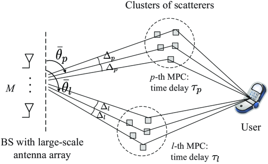
Figure 1: The clustered response model for multi-path environment, where each multi-path component consists of a continuum of indistinguishable rays.

II-A System Model

Let us consider a general finite scattering environment for massive MIMO systems shown in Fig. 1, where the BS is equipped with an $M\gg 1$ antennas and is located at an elevated position with few surrounding scatterers. The channel between BS and a user experiences frequency selective fading and the multi-path environment is characterized by the clustered response model [21]. The scatterers and reflectors are not located at all directions from the BS or the users but are grouped into several clusters with each cluster bouncing off a multi-path component (MPC) comprised of a continuum of simultaneous rays.

Without loss of generality, we suppose the propagation from a destined user to BS will go through $P$ resolvable independent multi-paths, and the mean AOA as well as the AS of the $p$-th MPC are denoted by $\bar{\vartheta}_{p}$ and $\Delta_{p}$, respectively. Then the corresponding $M\times 1$ uplink channel for the $p$-th MPC can be expressed by integrating over the incident angular region as

$$\mathbf{h}_{p}=\int_{\vartheta\in\mathcal{A}_{p}}\alpha(\vartheta)\mathbf{a}(\vartheta)d\vartheta=\int_{\bar{\vartheta}_{p}-\Delta_{p}}^{\bar{\vartheta}_{p}+\Delta_{p}}|\alpha(\vartheta)|e^{j\phi(\vartheta)}\mathbf{a}(\vartheta)d\vartheta,$$ (1)

where $\mathcal{A}_{p}\triangleq[\bar{\vartheta}_{p}-\Delta_{p},\bar{\vartheta}_{p}+\Delta_{p}]$ and $\alpha(\vartheta)\triangleq|\alpha(\vartheta)|e^{j\phi(\vartheta)}$ with $|\alpha(\vartheta)|$ and $\phi(\vartheta)$ representing the attenuation (amplitude) and phase of the incident signal ray coming from AOA $\vartheta$, respectively. Moreover, $\mathbf{a}(\vartheta)$ is the array manifold vector (AMV) or array response vector, whose expression is dependent on the specific array geometries. When a ULA is deployed, there is

$$\mathbf{a}(\vartheta)=\frac{1}{\sqrt{M}}\left[1,e^{-j\chi\cos(\vartheta)},e^{-j2\chi\cos(\vartheta)},\ldots,e^{-j(M-1)\chi\cos(\vartheta)}\right]^{T},$$ (2)

where $\chi\triangleq 2\pi fd/c$, $d$ denotes the antenna spacing, $f$ is the carrier frequency and $c$ is the speed of light. Obviously, $\mathbf{a}(\vartheta)$ is dependent on the signal carrier frequency $f$. Then the channel frequency response of the user can be written as [22]

$$\mathbf{h}(f) =\sum_{p=1}^{P}\mathbf{h}_{p}\cdot e^{-j2\pi f\tau_{p}}=\sum_{p=1}^{P}e^{-j2\pi f\tau_{p}}\int_{\mathcal{A}_{p}}\alpha(\vartheta)\mathbf{a}(\vartheta)d\vartheta,$$ (3)

where $\tau_{p}$ is the time delay of the $p$-th MPC.

From above channel model, the $M\times M$ CCM of the $p$-th MPC $\mathbf{h}_{p}$ can be written as

$$\mathbf{R}_{p}=\int_{\vartheta\in\mathcal{A}_{p}}\mathbb{E}\{|\alpha(\vartheta)|^{2}\}\mathbf{a}(\vartheta)\mathbf{a}^{H}(\vartheta)d\vartheta=\int_{\bar{\vartheta}_{p}-\Delta_{p}}^{\bar{\vartheta}_{p}+\Delta_{p}}S_{p}(\vartheta)\mathbf{a}(\vartheta)\mathbf{a}^{H}(\vartheta)d\vartheta,$$ (4)

where $S_{p}(\vartheta)\triangleq\mathbb{E}\{|\alpha(\vartheta)|^{2}\}$ denotes the PAS of $\mathbf{h}_{p}$, characterizing the channel power distribution of the $p$-th MPC in angular domain. Obvious, $\mathbf{R}_{p}$ is determined by the values of central AOA $\bar{\vartheta}_{p}$, AS $\Delta_{p}$, PAS $S_{p}(\vartheta)$, as well as the AMV $\mathbf{a}(\vartheta)$. Accordingly, if ULA is deployed, the $(m,n)$-th element of $\mathbf{R}_{p}$ is denoted by

$$[\mathbf{R}_{p}]_{m,n}=\frac{1}{M}\int_{\bar{\vartheta}_{p}-\Delta_{p}}^{\bar{\vartheta}_{p}+\Delta_{p}}S_{p}(\vartheta)e^{-j(m-n)\chi\cos(\vartheta)}d\vartheta.$$ (5)

II-B Representation and Expansion of CCM

Since $S_{p}(\vartheta)$ is also a function of the angle parameters $\bar{\vartheta}_{p}$ and $\Delta_{p}$, the estimation of $\mathbf{R}_{p}$ actually boils down to two sub-problems: angle estimation and PAS estimation. For angle acquisition, many canonical means such as various MUSIC [23] or ESPRIT methods [24], or some emerging approaches for large-scale antenna arrays like compressive sensing (CS) [25, 26] or discrete Fourier transform (DFT) [12] are available, whose detailed exposition will be left in Section III. Let us here focus on the analysis of PAS.

II-B1 Known PAS Distribution

If the prior distribution of $S_{p}(\vartheta)$ is available, then the expression of $[\mathbf{R}_{p}]_{m,n}$ in (5) could be possibly simplified to a function of $\bar{\vartheta}_{p}$ and $\Delta_{p}$. For example, if $S_{p}(\vartheta)$ is uniformly distributed with mean AOA $\bar{\vartheta}_{p}$ and AS $\Delta_{p}$, i.e., $S_{p}(\vartheta)=\frac{1}{2\Delta_{p}}$ for $\forall\vartheta\in[\bar{\vartheta}_{p}-\Delta_{p},\bar{\vartheta}_{p}+\Delta_{p}]$ [18], then the $(m,n)$-th entry of $\mathbf{R}_{p}$ can be expressed as

$$[\mathbf{R}_{p}]_{m,n} =\frac{1}{2M\Delta_{p}}\int_{\bar{\vartheta}_{p}-\Delta_{p}}^{\bar{\vartheta}_{p}+\Delta_{p}}e^{-j(m-n)\chi\cos(\vartheta)}d\vartheta$$ (6a)

$$\approx\frac{1}{2M\Delta_{p}}e^{-j(m-n)\chi\cos(\bar{\vartheta}_{p})}\int_{-\Delta_{p}}^{\Delta_{p}}e^{j(m-n)\chi\sin(\bar{\vartheta}_{p})\vartheta}d\vartheta$$

$$=\frac{1}{M}e^{-j\chi_{mn}\cos(\bar{\vartheta}_{p})}\text{sinc}\left(\chi_{mn}\Delta_{p}\sin(\bar{\vartheta}_{p})\right),$$ (6b)

where $\chi_{mn}\triangleq(m-n)\chi$ and $\text{sinc}(x)\triangleq\sin x/x$ denotes the sinc function. The second approximation equation derives from the Taylor expansion of $\cos(\vartheta)$ at $\bar{\vartheta}$, namely, $\cos(\vartheta)\approx\cos(\bar{\vartheta})-(\vartheta-\bar{\vartheta})\sin\bar{\vartheta}$. Similarly, if $S_{p}(\vartheta)$ is modeled by Laplacian distribution [27] as

$$S_{p}(\vartheta)=\frac{1}{\sqrt{2}\Delta_{p}}e^{-\frac{\sqrt{2}|\vartheta-\bar{\vartheta}_{p}|}{\Delta_{p}}},$$ (7)

then there is

$$[\mathbf{R}_{p}]_{m,n} =\int_{\bar{\vartheta}_{p}-\Delta_{p}}^{\bar{\vartheta}_{p}+\Delta_{p}}\frac{1}{\sqrt{2}M\Delta_{p}}e^{-\frac{\sqrt{2}}{\Delta_{p}}|\vartheta-\bar{\vartheta}_{p}|-j\chi_{mn}\cos(\vartheta)}d\vartheta$$ (8a)

$$\approx\frac{1}{\sqrt{2}M\Delta_{p}}e^{-j\chi_{mn}\cos(\bar{\vartheta}_{p})}\int_{-\Delta_{p}}^{\Delta_{p}}e^{-\frac{\sqrt{2}|\vartheta|}{\Delta_{p}}+j\chi_{mn}\sin(\bar{\vartheta}_{p})\vartheta}d\vartheta$$

$$=\frac{1}{\sqrt{2}M}e^{-j\chi_{mn}\cos(\bar{\vartheta}_{p})}\frac{1}{2+\chi_{mn}^{2}\Delta_{p}^{2}\sin^{2}(\bar{\vartheta})}\left\{2\sqrt{2}\left(1-e^{-\sqrt{2}}\cos\left(\chi_{mn}\Delta_{p}\sin(\bar{\vartheta})\right)\right)\right.$$

$$\left.+2e^{-\sqrt{2}}\chi_{mn}^{2}\Delta_{p}^{2}\sin^{2}(\bar{\vartheta})~{}\text{sinc}\left(\chi_{mn}\Delta_{p}\sin(\bar{\vartheta})\right)\right\}.$$ (8b)

Note that the closed-form equations (6b) and (8b) are the approximation of (6a) and (8a), respectively, under the condition of very narrow AS. That is to say, if the AS is not small enough, we should refer back to (6a) and (8a) for the true CCMs reconstruction. In this case, the basic Monte Carlo method may be adopted for the integral process and thus we refer to this procedure as the Monte Carlo integral CCM reconstruction (MC-iCCM) . In comparison, the closed-form equations (6b) and (8b) are referred to as the Closed-form integral CCM reconstruction (CF-iCCM) .

II-B2 Unknown PAS Distribution

Let us then consider a more practical case where the prior knowledge of the distribution of $S_{p}(\vartheta)$ is unavailable. Under this circumstance, $S_{p}(\vartheta)$ could not be explicitly expressed by a given probability density function and thereby $[\mathbf{R}_{p}]_{m,n}$ may not be simplified like equations (6) or (8).

Without any prior knowledge of $S_{p}(\vartheta)$, one should first estimate $S_{p}(\vartheta)$. With limited number of observations over antennas, we need first approximate $\mathbf{R}_{p}$ by an appropriate basis expansion model (BEM), or to approximate the integral of (4) by the sum of discrete points extracted from the angular integral region. For example, the whole spatial space is often discretized evenly into $M$ blocks, each with the width of $\frac{2\pi}{M}$, and then the basis vectors could be chosen as the columns of an $M\times M$ DFT matrix when ULA is deployed at BS. In this case, the continuous PAS function in (4) should be approximated by $M$ discrete expansion coefficients, denoted as $\{S_{p,l}\}$ for $l=0,1,\ldots,M-1$. Then, there is

$$\mathbf{R}_{p}=\int_{\bar{\vartheta}_{p}-\Delta_{p}}^{\bar{\vartheta}_{p}+\Delta_{p}}S_{p}(\vartheta)\mathbf{a}(\vartheta)\mathbf{a}^{H}(\vartheta)d\vartheta\approx\sum_{l=0}^{M-1}S_{p,l}\mathbf{f}_{l}\mathbf{f}_{l}^{H}=\mathbf{F}\text{diag}\left\{S_{p,0},S_{p,1},\ldots,S_{p,M-1}\right\}\mathbf{F}^{H},$$ (9)

where $\mathbf{F}$ is the $M\times M$ normalized DFT matrix whose $(p,q)$-th element is $\left[\mathbf{F}\right]_{p,q}=e^{-j\frac{2\pi}{M}pq}/\sqrt{M}$ and $\mathbf{f}_{l}$ is the $l$-th column of $\mathbf{F}$. Therefore, $S_{p,l}$ is given as

$$S_{p,l} \approx\mathbf{f}_{l}^{H}\mathbf{R}_{p}\mathbf{f}_{l}=\int_{\bar{\vartheta}_{p}-\Delta_{p}}^{\bar{\vartheta}_{p}+\Delta_{p}}S_{p}(\vartheta)\mathbf{f}_{l}^{H}\mathbf{a}(\vartheta)\mathbf{a}^{H}(\vartheta)\mathbf{f}_{l}d\vartheta.$$ (10)

The estimation of PAS is thus equivalent to estimating the $M$ expansion coefficients $\{S_{p,l}\}_{l=1}^{M}$.

A more accurate way other than using DFT expansion is to approximate $\mathbf{R}_{p}$ with non-orthogonal basis vectors within the actual incident AS. For instance, without any prior knowledge of $S_{p}(\vartheta)$, a natural idea is to sample $S_{p}(\vartheta)$ at discrete points, e.g., $\{S_{p}(\vartheta_{l})|\vartheta_{l}\in\mathcal{A}_{p},l=0,1,\ldots,L-1\}$. Then the approximation of $\mathbf{R}_{p}$ could be expressed as

$$\mathbf{R}_{p}=\int_{\bar{\vartheta}_{p}-\Delta_{p}}^{\bar{\vartheta}_{p}+\Delta_{p}}S_{p}(\vartheta)\mathbf{a}(\vartheta)\mathbf{a}^{H}(\vartheta)d\vartheta\approx\sum_{l=0,\forall\vartheta_{l}\in\mathcal{A}_{p}}^{L-1}S_{p}(\vartheta_{l})\mathbf{a}(\vartheta_{l})\mathbf{a}^{H}(\vartheta_{l}).$$ (11)

It is apparent that $S_{p}(\vartheta_{l})$ is slightly different from $S_{p,l}$ in (10). As we increase the number of sum terms $L$ in (11), $S_{p}(\vartheta_{l})$’s is a more accurate approximation of the continuous PAS $S_{p}(\vartheta)$ and thus renders a more accurate CCM approximation.

In these cases, to reconstruct CCMs, not only the central AOA $\bar{\vartheta}_{p}$ and AS $\Delta_{p}$ but also the discrete samples of PAS $S_{p}(\vartheta_{l})$’s are needed.

II-C Inferring Downlink CCMs from Uplink CCMs

Since the AMV $\mathbf{a}(\vartheta)$ is dependent on the signal carrier frequencies, downlink CCMs will differ from their uplink counterparts in FDD systems. Denote the uplink and downlink signal carrier frequencies by $f_{u}$ and $f_{d}$ respectively. Meanwhile, let us rewrite the uplink AMV $\mathbf{a}(\vartheta)$ and CCM $\mathbf{R}_{p}$ as $\mathbf{a}_{u}(\vartheta)$ and $\mathbf{R}_{p}^{u}$, respectively and represent their downlink ones accordingly as $\mathbf{a}_{d}(\vartheta)$ and $\mathbf{R}_{p}^{d}$. Then, there are

$$\mathbf{R}_{p}^{u} =\int_{\vartheta\in\mathcal{A}^{u}_{p}}S^{u}_{p}(\vartheta)\mathbf{a}_{u}(\vartheta)\mathbf{a}_{u}^{H}(\vartheta)d\vartheta,$$ (12)

$$\mathbf{R}_{p}^{d} =\int_{\vartheta\in\mathcal{A}^{d}_{p}}S^{d}_{p}(\vartheta)\mathbf{a}_{d}(\vartheta)\mathbf{a}_{d}^{H}(\vartheta)d\vartheta,$$ (13)

where $\mathcal{A}_{p}^{d}$ is the downlink angle of departure (AOD) interval at BS and $S_{p}^{d}(\vartheta)$ is the downlink PAS. Considering the structure of $\mathbf{a}_{u}(\vartheta)$ and $\mathbf{a}_{d}(\vartheta)$, the following transformation holds:

$$\mathbf{a}_{d}(\vartheta)=\mathbf{\Theta}(\vartheta)\mathbf{a}_{u}(\vartheta),$$ (14)

with $\mathbf{\Theta}(\vartheta)$ defined as

$$\mathbf{\Theta}(\vartheta)\triangleq\text{diag}\left\{1,e^{-j\frac{2\pi d}{c}(f_{d}-f_{u})\cos(\vartheta)},e^{-j\frac{2\pi d}{c}(f_{d}-f_{u})2\cos(\vartheta)},\ldots,e^{-j\frac{2\pi d}{c}(f_{d}-f_{u})(M-1)\cos(\vartheta)}\right\}.$$ (15)

To proceed, we adopt the following assumptions from many theoretical works [15, 16, 19, 28, 7] and measurement tests [29, 30, 31, 33, 32]:

1. The underlying angle parameters of uplink and downlink channels are reciprocal, i.e, $\mathcal{A}_{p}^{d}\approx\mathcal{A}^{u}_{p}$, as long as the uplink and downlink frequency discrepancy is not big.

2. The PAS of uplink and downlink channels are reciprocal, except for a frequency dependent scalar $\mu$, i.e., $S_{p}^{d}(\vartheta)=\mu S^{u}_{p}(\vartheta)$. That is, the shapes of uplink/downlink PAS functions are the same.

Based on these facts, the relationship between uplink/downlink CCMs can be derived as

$$\mathbf{R}_{p}^{d}=\int_{\bar{\vartheta}_{p}-\Delta_{p}}^{\bar{\vartheta}_{p}+\Delta_{p}}\mu S^{u}_{p}(\vartheta)\mathbf{\Theta}(\vartheta)\mathbf{a}_{u}(\vartheta)\mathbf{a}_{u}^{H}(\vartheta)\mathbf{\Theta}^{H}(\vartheta)d\vartheta.$$ (16)

By combining (11) and (14), the discrete approximation of (16) is given by

$$\mathbf{R}_{p}^{d}\approx\sum_{l=0,\forall\vartheta_{l}\in\mathcal{A}^{u}_{p}}^{L-1}\mu S^{u}_{p}(\vartheta_{l})\mathbf{a}_{d}(\vartheta_{l})\mathbf{a}_{d}^{H}(\vartheta_{l})=\sum_{l=0,\forall\vartheta_{l}\in\mathcal{A}^{u}_{p}}^{L-1}\mu S^{u}_{p}(\vartheta_{l})\mathbf{\Theta}(\vartheta_{l})\mathbf{a}_{u}(\vartheta_{l})\mathbf{a}_{u}^{H}(\vartheta_{l})\mathbf{\Theta}^{H}(\vartheta_{l}).$$ (17)

Following above analysis, it is clear that the uplink angle parameters and PAS could be used to infer the downlink CCM, even in FDD systems.

III Proposed Channel Estimation Scheme

As shown in Fig. 2, the proposed transmission starts from an uplink preamble phase to obtain all users’ initial AS information, which will be used for initial user grouping and scheduling. In the subsequent transmissions, the instantaneous channel estimates are updated with limited pilots, and users’ angle information are also dynamically updated. Then, the uplink/downlink CCMs are reconstructed and utilized to enhance the channel estimation via minimum mean square error (MMSE) estimators. The flow chart of the overall transmission scheme is presented in Fig. 3 for better understanding.

For ease of illustration, we here will only focus on channel estimation for the $p$-th MPC of all users. Meanwhile, we use an additional subscript $k$ to indicate all the symbols for user-$k$.

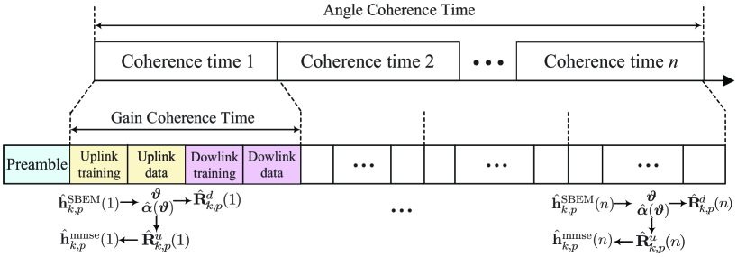
Figure 2: Transmission phase of our proposed scheme.

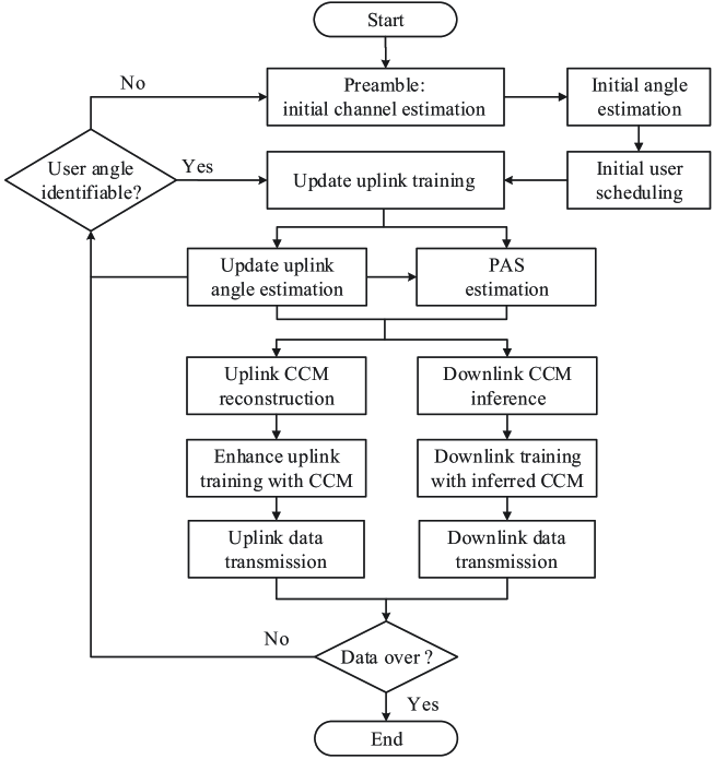
Figure 3: The flow chart of our proposed scheme.

III-A Preamble For Initial Angle Estimation and User Scheduling

During the preamble phase, all $K$ users adopt the conventional uplink training methods, e.g., least square (LS), to estimate their initial CSI $\hat{\mathbf{h}}^{\text{ini}}_{k,p}$, $k=1,\ldots,K$. The next step is to extract the initial $\mathcal{A}_{k,p}$ of each user from $\hat{\mathbf{h}}^{\text{ini}}_{k,p}$.

III-A1 Initial Angle Estimation

Owing to the narrow AS, namely, $\Delta_{k,p}$ is small (especially, $\Delta_{k,p}$ is zero in mmWave scenarios [7]), $\mathbf{h}_{k,p}$ in (1) will exhibit sparsity or low-rank property in the angle domain and thus it could be approximately represented by discretizing the integral of (1) as

$$\mathbf{h}_{k,p}=\mathbf{A}\bm{\alpha},$$ (18)

where $\mathbf{A}=[\mathbf{a}(\theta_{0}),\mathbf{a}(\theta_{1}),\ldots,\mathbf{a}(\theta_{L-1})]\in\mathbb{C}^{M\times L}$ with $\{\theta_{l}\}_{l=0}^{L-1}\in[-\pi,\pi]$ is an angle domain transform matrix. Note that, here the possible range of unknown $\theta_{l}$ belongs to $[-\pi,\pi]$, different from the range of true angles $\vartheta\in\mathcal{A}_{k,p}$. Moreover, $\bm{\alpha}\in\mathbb{C}^{L\times 1}$ is the sparse representation to be determined and only a few components of $\bm{\alpha}$ corresponding to those angles inside $\mathcal{A}_{k,p}$ are nonzero. Therefore, the nonzero components of $\bm{\alpha}$ could facilitate the estimation of AOA interval $\mathcal{A}_{k,p}$. To this end, the initial angle estimation problem is formulated as

$$\left[\hat{\bm{\alpha}},\{\hat{\theta}_{l}\}^{L-1}_{l=0}\right]=\operatorname*{argmin}_{\bm{\alpha},~{}\{\theta_{l}\}^{L-1}_{l=0}}\ \|\hat{\mathbf{h}}^{\text{ini}}_{k,p}-\mathbf{A}\bm{\alpha}\|^{2}.$$ (19)

To solve this problem, there are several common options. First, we can resort to maximum likelihood (ML) [34] method to search for the optimal angle candidates $\{\hat{\theta}_{l}\}_{l=0}^{L-1}$. Second, if $L\gg M$, the super-resolution CS [25, 26] is a popular and suitable choice for such kind of sparse recovery problem. The spatial rotation enhanced DFT method from array signal processing in [12] is also a good choice. Among the three options, ML and CS methods are capable of achieving high angle estimation accuracy. Nevertheless, ML requires exhaustive search in the whole angle range $[-\pi,\pi]$, while CS relies on non-linear optimization and iterations, both of which suffer from relatively high complexity. By contrast, the spatial rotation enhanced DFT method achieves a nice tradeoff between angle estimation accuracy and computational complexity. In this paper, we adopt the third option for angle acquisition.

According to [12], $\mathbf{A}$ is chosen as $\mathbf{A}=\mathbf{\Phi}^{H}(\psi)\mathbf{F}^{H}$, with the spatial rotation matrix $\mathbf{\Phi}(\psi)$ defined as $\mathbf{\Phi}(\psi)=\textup{diag}\left\{[1,e^{j\psi},\cdots,e^{j(M-1)\psi}]\right\}$ for $\psi\in[-\frac{\pi}{M},\frac{\pi}{M}]$. In doing so, (19) is equivalent to $\min_{\bm{\alpha},\{\theta_{l}\}^{L-1}_{l=0},\psi}\|\hat{\mathbf{h}}^{\text{ini}}_{k,p}-\mathbf{\Phi}^{H}(\psi)\mathbf{F}^{H}\bm{\alpha}\|^{2}$, and then the angle estimation problem is boiled down to determining the optimal spatial rotation parameter $\psi_{k,p}$ and the corresponding index set $\mathcal{Q}_{k,p}$ of nonzero components of $\bm{\alpha}$, namely,

$$[\psi_{k,p},\mathcal{Q}_{k,p}]=\operatorname*{argmax}_{\psi,\ \mathcal{Q}}\quad \Big{\|}\left[\mathbf{F}\mathbf{\Phi}(\psi)\hat{\mathbf{h}}^{\text{ini}}_{k,p}\right]_{\mathcal{Q},:}\Big{\|}^{2}\quad\text{s.t.}\quad|\mathcal{Q}|=\kappa,$$ (20)

where $\kappa$ is a pre-determined largest cardinality of $\mathcal{Q}$. Afterwards, the AOA range of user-$k$ could be inferred from the indices inside $\mathcal{Q}_{k,p}$ according to Lemma 1 in [12] as

$$\hat{\mathcal{A}}_{k,p}=\left\{\vartheta\Big{|}\left(\frac{f_{u}d}{2\pi c}\psi_{k,p}-\frac{qc}{Mf_{u}d}\right)_{\min}\leq\cos(\vartheta)\leq\left(\frac{f_{u}d}{2\pi c}\psi_{k,p}-\frac{qc}{Mf_{u}d}\right)_{\max},\forall q\in\mathcal{Q}_{k,p}\right\}.$$ (21)

Therefore, $\widehat{\bar{\vartheta}_{k,p}}$ and $\hat{\Delta}_{k,p}$ are obtained accordingly.

III-A2 Initial User Scheduling

After obtaining the AOA intervals of all users, we divide users into different groups, denoted by $\mathcal{U}_{1},\mathcal{U}_{2},\ldots$, such that users with non-overlapped AOA intervals, i.e., $\hat{\mathcal{A}}_{k,p}$ or $\mathcal{Q}_{k,p}$, stay in the same group, as shown in Fig. 4. According to [6, 5, 12], users in the same group could reuse the same training sequence in the subsequent channel updating without causing pilot contamination, while different groups still adopt orthogonal training sequences to remove the inter-group interference. Such an angle domain grouping strategy will significantly reduce the subsequent training overhead (after preamble) and is called as angle-division multiple access (ADMA).

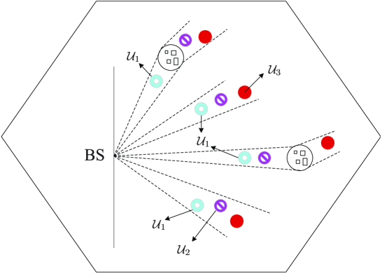
Figure 4: Illustration of ADMA user scheduling, where users (circles) with the same shape are in the same group and can reuse the same orthogonal training sequence.

III-B Uplink Channel Estimation with CCM Reconstruction

III-B1 Instantaneous Channel Update

After ADMA user scheduling, the subsequent instantaneous channel update for all users could be implemented with the spatial basis expansion model (SBEM) scheme proposed by [12], which resorts to the full utilization of the angular information. Take users in group $\mathcal{U}_{1}$ for instance and denote the orthogonal training sequence assigned to $\mathcal{U}_{1}$ as $\mathbf{s}_{1}$ with $\mathbf{s}_{1}^{H}\mathbf{s}_{1}=\rho_{u}$, where $\rho_{u}$ is the total uplink training SNR. Then at the $n$-th ($n=1,2,\ldots,N$) coherence time interval, the received signals at BS from users in $\mathcal{U}_{1}$ are expressed as

$$\mathbf{Y}_{\mathcal{U}_{1}}(n)=\sum_{\begin{subarray}{c}i\in\mathcal{U}_{1}\end{subarray}}\mathbf{h}_{i,p}(n)\mathbf{s}_{1}^{H}+\mathbf{N},$$ (22)

where $\mathbf{N}$ is a Gaussian noise matrix with $\mathcal{CN}(0,1)$ elements. The inter-group interference does not appear due to the orthogonal training among different groups. The uplink channel estimate for all users in $\mathcal{U}_{1}$ is then computed as

$$\hat{\mathbf{h}}_{\mathcal{U}_{1}}(n)=\frac{1}{\rho_{u}}\mathbf{Y}_{\mathcal{U}_{1}}(n)\mathbf{s}_{1}=\mathbf{h}_{k,p}(n)+\sum_{\begin{subarray}{c}i\neq k;i,k\in\mathcal{U}_{1}\end{subarray}}\mathbf{h}_{i,p}(n)+\frac{1}{\sqrt{\rho_{u}}}\mathbf{n}_{k,p},$$ (23)

with $\mathbf{n}_{k,p}\sim\mathcal{CN}(\mathbf{0},\mathbf{I}_{M})$ denoting the normalized noise vector. Since users in $\mathcal{U}_{1}$ have disjoint AOA intervals, the second term in (23) could be eliminated for the $k$-th user by only extracting the components of $\hat{\mathbf{h}}_{\mathcal{U}_{1}}(n)$ indexed by $\mathcal{Q}_{k,p}$. Specifically, we have

$$\left[\mathbf{F}\mathbf{\Phi}(\psi_{k,p}(n{-}1))\hat{\mathbf{h}}_{\mathcal{U}_{1}}(n)\right]_{\mathcal{Q}_{k,p}(n{-}1),:}=\left[\mathbf{F}\mathbf{\Phi}(\psi_{k,p}(n{-}1))\mathbf{h}_{k,p}(n)\right]_{\mathcal{Q}_{k,p}(n{-}1),:}$$

$$\kern 40.0pt+\sum_{\begin{subarray}{c}i\neq k;i,k\in\mathcal{U}_{1}\end{subarray}}\left[\mathbf{F}\mathbf{\Phi}(\psi_{k,p}(n{-}1))\mathbf{h}_{i,p}(n)\right]_{\mathcal{Q}_{k,p}(n{-}1),:}+\frac{1}{\sqrt{\rho_{u}}}\left[\mathbf{F}\mathbf{\Phi}(\psi_{k,p}(n{-}1))\mathbf{n}_{k,p}\right]_{\mathcal{Q}_{k,p}(n{-}1),:}$$

$$\kern 40.0pt\approx\left[\mathbf{F}\mathbf{\Phi}(\psi_{k,p}(n{-}1))\mathbf{h}_{k,p}(n)\right]_{\mathcal{Q}_{k,p}(n{-}1),:}+\frac{1}{\sqrt{\rho_{u}}}\left[\mathbf{F}\mathbf{\Phi}(\psi_{k,p}(n{-}1))\mathbf{n}_{k,p}\right]_{\mathcal{Q}_{k,p}(n{-}1),:}.$$ (24)

Note that the parameters $\psi_{k,p}(n{-}1)$ and $\mathcal{Q}_{k,p}(n{-}1)$ from the $(n{-}1)$-th coherence time are adopted for the current channel update, because each user’s AOA interval is unlikely to change much in a short time slot. Then user-$k$’s uplink channel update could be recovered from (III-B1) by the following equation:

$$\hat{\mathbf{h}}_{k,p}^{\text{SBEM}}(n)=\mathbf{\Phi}(\psi_{k,p}(n{-}1))^{H}\left[\mathbf{F}^{H}\right]_{:,\mathcal{Q}_{k,p}(n{-}1)}\left[\mathbf{F}\mathbf{\Phi}(\psi_{k,p}(n{-}1))\hat{\mathbf{h}}_{\mathcal{U}_{1}}(n)\right]_{\mathcal{Q}_{k,p}(n{-}1),:}.$$ (25)

III-B2 Instantaneous Angle Update

With updated instantaneous channels, we are able to update the instantaneous $\hat{\mathcal{A}}_{k,p}(n)$, $\mathcal{Q}_{k,p}(n)$ and $\psi_{k,p}(n)$ from $\hat{\mathbf{h}}^{\text{SBEM}}_{k,p}(n)$, according to the same procedures of (20) in preamble phase. This updated angle information actually helps to monitor the motion of users and thus triggers a user re-scheduling process when two users’ angular distance becomes smaller than a certain threshold, as indicated by the flow chart in Fig. 3.

III-B3 PAS Estimation

As mentioned in Section II-B, we need to estimate the discrete PAS $S_{k,p}(\vartheta)$ for $\vartheta\in\hat{\mathcal{A}}_{k,p}(n)$. Since only one instantaneous channel realization is obtained, we will first estimate $\hat{\alpha}(\vartheta)$ from $\hat{\mathbf{h}}^{\text{SBEM}}_{k,p}(n)$ and then use $|\hat{\alpha}(\vartheta)|^{2}$ to approximate the expectation $S_{k,p}(\vartheta)=\mathbb{E}\{|\alpha(\vartheta)|^{2}\}$.

The nonzero components of $\hat{\bm{\alpha}}$ in (19) could have been used to estimate the desired $S_{p}(\theta_{l})$ at their corresponding angles $\theta_{l}$. However, the selected angles $\{\theta_{l}\}_{l=0}^{L-1}$ in (19) are chosen from $[-\pi,\pi]$, not from $\hat{\mathcal{A}}_{k,p}(n)$. In other words, only few angles among $\{\theta_{l}\}_{l=0}^{L-1}$ will be located inside $\hat{\mathcal{A}}_{k,p}(n)$ and thus the number of nonzero components of $\hat{\bm{\alpha}}$ in (19) is not sufficient to get an accurate estimation of the continuous PAS $S_{k,p}(\vartheta)$ for $\vartheta\in\hat{\mathcal{A}}_{k,p}(n)$, as indicated in (11). In line of this thought, we should first determine enough discrete angles of interest inside $\hat{\mathcal{A}}_{k,p}(n)$ and then estimate the corresponding instantaneous channel gains. Specifically, with updated instantaneous channel $\hat{\mathbf{h}}^{\text{SBEM}}_{k,p}(n)$ as well as estimated angle parameters $\hat{\mathcal{A}}_{k,p}(n)$, $\widehat{\bar{\vartheta}_{k,p}}(n)$ and $\hat{\Delta}_{k,p}(n)$, the acquisition of instantaneous channel gains corresponding to selected angles inside $\hat{\mathcal{A}}_{k,p}(n)$ could be formulated as

$$\hat{\bm{\alpha}}(\bm{\vartheta})=\operatorname*{argmin}_{\bm{\alpha}(\bm{\vartheta})}\quad\|\hat{\mathbf{h}}^{\text{SBEM}}_{k,p}(n)-\mathbf{\Phi}^{H}(\psi_{k,p}(n))\mathbf{A}(\bm{\vartheta})\bm{\alpha}(\bm{\vartheta})\|^{2},$$ (26)

where $\bm{\vartheta}=[\vartheta_{0},\vartheta_{1},\ldots,\vartheta_{L-1}]^{T}$ collects $L$ discrete angles of interest selected from $\hat{\mathcal{A}}_{k,p}(n)$. One simple way to determine these $L$ discrete angles is to pick $L$ evenly spaced angles inside $\hat{\mathcal{A}}_{k,p}(n)$, namely, $\vartheta_{l}=\widehat{\bar{\vartheta}_{k,p}}(n)-\hat{\Delta}_{k,p}(n)+\frac{2\hat{\Delta}_{k,p}(n)l}{L}$ for $l=0,\ldots,L-1$. Moreover, $\mathbf{A}$ in (19) is replaced by $\mathbf{A}(\bm{\vartheta})\triangleq[\mathbf{a}(\vartheta_{0}),\mathbf{a}(\vartheta_{1}),\ldots,\mathbf{a}(\vartheta_{L-1})]$, and $\hat{\bm{\alpha}}(\bm{\vartheta})=[\hat{\alpha}(\vartheta_{0}),\hat{\alpha}(\vartheta_{1}),\ldots,\hat{\alpha}(\vartheta_{L-1})]^{T}$ is exactly our desired instantaneous channel gains.

To solve the problem in (26), we have to consider two cases. When $L\leq M$, $\mathbf{A}(\bm{\vartheta})\in\mathbb{C}^{M\times L}$ is a tall matrix and the solution of $\hat{\bm{\alpha}}(\bm{\vartheta})$ could be directly obtained by LS as

$$\hat{\bm{\alpha}}(\bm{\vartheta})=\mathbf{A}^{{\dagger}}(\bm{\vartheta})\mathbf{\Phi}(\psi_{k,p}(n))\hat{\mathbf{h}}^{\text{SBEM}}_{k,p}(n).$$ (27)

On the other side, a large $L~{}(\geq M)$ may generally be considered to get dense angle samples inside $\hat{\mathcal{A}}_{k,p}(n)$ such that $|\hat{\alpha}(\vartheta)|^{2}$ may give a more accurate approximation of the continuous $S_{k,p}(\vartheta)$. Unfortunately, due to more unknown variables than the observations, LS method is not applicable for (26). To find an alternative solution, let us consider (26) from another perspective. If we take the ideal channel vector $\mathbf{h}_{k,p}(n)$ as an $M$-point receiving vector in the spatial domain, the values of $\bm{\alpha}(\bm{\vartheta})$ are exactly the outputs of the discrete time Fourier transform (DTFT) of $\mathbf{\Phi}(\psi_{k,p}(n))\mathbf{h}_{k,p}(n)$ at certain angles. To be concrete, the DTFT of $\mathbf{\Phi}(\psi_{k,p}(n))\mathbf{h}_{k,p}(n)$ could be given as

$$\beta(\xi) \triangleq\frac{1}{\sqrt{M}}\sum_{m=0}^{M-1}[\mathbf{\Phi}(\psi_{k,p}(n))\mathbf{h}_{k,p}(n)]_{m}e^{-jm\xi}=\frac{1}{M}\int_{\vartheta\in\mathcal{A}_{k,p}(n)}\alpha(\vartheta)\sum_{m=0}^{M-1}e^{-j\chi m\cos(\vartheta)+jm\psi_{k,p}(n)-jm\xi}d\vartheta$$

$$=\int_{\vartheta\in\mathcal{A}_{k,p}(n)}\alpha(\vartheta)~{}\frac{\sin\left[\left(\chi\cos(\vartheta)-\psi_{k,p}(n)+\xi\right)\frac{M}{2}\right]}{M\sin\left[\left(\chi\cos(\vartheta)-\psi_{k,p}(n)+\xi\right)\frac{1}{2}\right]}e^{-j\frac{M-1}{2}\left(\chi\cos(\vartheta)-\psi_{k,p}(n)+\xi\right)}d\vartheta$$

$$=\int_{\vartheta\in\mathcal{A}_{k,p}(n)}\alpha(\vartheta)~{}\text{asinc}_{M}\left(\chi\cos(\vartheta)-\psi_{k,p}(n)+\xi\right)e^{-j\frac{M-1}{2}\left(\chi\cos(\vartheta)-\psi_{k,p}(n)+\xi\right)}d\vartheta,$$ (28)

where $\text{asinc}_{M}(x)\triangleq\frac{\sin(Mx/2)}{M\sin(x/2)}$ is an aliased sinc function, $\beta(\xi)$ is the DTFT output and the scalar variable $\xi\in[-\pi,\pi]$ could be deemed as spatial frequency. Since that $\text{asinc}_{M}(0)=1$ and $|\text{asinc}_{M}(x)|\leq\frac{1}{M|x|}$ for $x\neq 0$, there is

$$\beta(\xi)\big{|}_{\xi=\psi_{k,p}(n)-\chi\cos(\vartheta)}\to\alpha(\vartheta),\ \forall\vartheta\in\mathcal{A}_{k,p}(n),\ \text{as}\ M\to\infty.$$ (29)

which indicates that as $\xi$ varies across the whole spatial frequency range, $\beta(\xi)$ gives an accurate estimation for $\alpha(\vartheta),~{}\forall\vartheta\in\mathcal{A}_{k,p}(n)$. When $L$ discrete angles $\bm{\vartheta}=[\vartheta_{0},\vartheta_{1},\ldots,\vartheta_{L-1}]^{T}$ is considered, the desired $\hat{\bm{\alpha}}(\bm{\vartheta})=[\hat{\alpha}(\vartheta_{0}),\hat{\alpha}(\vartheta_{1}),\ldots,\hat{\alpha}(\vartheta_{L-1})]^{T}$ are exactly the sampling results of $\beta(\xi)$ at corresponding spatial frequencies, namely, $\bm{\beta}(\bm{\xi})\triangleq[\beta(\xi_{0}),\beta(\xi_{1}),\ldots,\beta(\xi_{L-1})]^{T}$, with $\xi_{l}=\psi_{k,p}(n)-\chi\cos(\vartheta_{l})$ for $l=0,\ldots,L-1$. According to (III-B3), the expression of $\bm{\beta}(\bm{\xi})$ could be further specified as

$$\bm{\beta}(\bm{\xi})=\bm{\Psi}\mathbf{\Phi}(\psi_{k,p}(n))\mathbf{h}_{k,p}(n),$$ (30)

where $\bm{\Psi}\in\mathbb{C}^{L\times M}$ is defined as

$$\bm{\Psi}\triangleq\left[\begin{array}[]{cccc}1&e^{-j\xi_{0}}&\cdots&e^{-j(M-1)\xi_{0}}\\ 1&e^{-j\xi_{1}}&\cdots&e^{-j(M-1)\xi_{1}}\\ \vdots&\vdots&\ddots&\vdots\\ 1&e^{-j\xi_{L-1}}&\cdots&e^{-j(M-1)\xi_{L-1}}\end{array}\right].$$ (35)

Therefore, the instantaneous channel gain estimates $\hat{\bm{\alpha}}(\bm{\vartheta})$ under the condition of $L\geq M$ can be expressed as

$$\hat{\bm{\alpha}}(\bm{\vartheta})=\bm{\Psi}\mathbf{\Phi}(\psi_{k,p}(n))\hat{\mathbf{h}}^{\text{SBEM}}_{k,p}(n).$$ (36)

III-B4 Uplink CCM Reconstruction

In the sequel, we show how to reconstruct the uplink CCMs with the obtained uplink angles $\hat{\mathcal{A}}_{k,p}(n)$ and channel gains $\hat{\bm{\alpha}}(\bm{\vartheta})$. Let us model the random channel phases of all signal rays as independent uniformly distributed variables in $[-\pi,\pi]$, and then along with the estimated channel gains, we may artificially generate many copies of instantaneous uplink channel estimates. In particular, we generate the auxiliary uplink channel estimates with random additional phase as

$$\mathbf{h}_{k,p}^{\text{aux}}(n)=\int_{\hat{\mathcal{A}}_{k,p}(n)}|\hat{\alpha}(\vartheta)|e^{j\phi(\vartheta)+j\widetilde{\phi}(\vartheta)}\mathbf{a}(\vartheta)d\vartheta,$$ (37)

where $\widetilde{\phi}(\vartheta)$ is the modeled random phase for the incident ray from AOA $\vartheta$, and $\widetilde{\phi}(\vartheta_{i})$ and $\widetilde{\phi}(\vartheta_{j})$ are mutually independent for any $\vartheta_{i},\vartheta_{j}\in\hat{\mathcal{A}}_{k,p}(n)$ and $\vartheta_{i}\neq\vartheta_{j}$. Approximating the integral of (37) with the discrete angles $\bm{\vartheta}$ and the estimated channel gains $\hat{\bm{\alpha}}(\bm{\vartheta})$ in (26), we obtain

$$\mathbf{h}_{k,p}^{\text{aux}}(n) \approx\sum_{l=0}^{L-1}\hat{\alpha}(\vartheta_{l})e^{j\widetilde{\phi}(\vartheta_{l})}\mathbf{\Phi}^{H}(\psi_{k,p}(n))\mathbf{a}(\vartheta_{l})=\mathbf{\Phi}^{H}(\psi_{k,p}(n))\mathbf{A}(\bm{\vartheta})\mathbf{\Pi}(\bm{\vartheta})\hat{\bm{\alpha}}(\bm{\vartheta})$$

$$=\mathbf{\Phi}^{H}(\psi_{k,p}(n))\mathbf{A}(\bm{\vartheta})\mathbf{\Pi}(\bm{\vartheta})\bm{\Psi}\mathbf{\Phi}(\psi_{k,p}(n))\hat{\mathbf{h}}^{\text{SBEM}}_{k,p}(n),$$ (38)

where $\mathbf{\Pi}(\bm{\vartheta})\triangleq\text{diag}\big{\{}\widetilde{\phi}(\vartheta_{0}),\widetilde{\phi}(\vartheta_{1}),\ldots,\widetilde{\phi}(\vartheta_{L-1})\big{\}}$ collects the random phases. To reconstruct the CCM $\hat{\mathbf{R}}^{u}_{k,p}(n)$, we take the expectation of $\mathbf{h}_{k,p}^{\text{aux}}(n)$ and obtain

$$\hat{\mathbf{R}}^{u}_{k,p}(n) =\mathbb{E}\left\{\mathbf{h}_{k,p}^{\text{aux}}(n)\mathbf{h}_{k,p}^{\text{aux}}(n)^{H}\right\}$$

$$=\mathbb{E}\left\{\mathbf{\Phi}^{H}(\psi_{k,p}(n))\mathbf{A}(\bm{\vartheta})\mathbf{\Pi}(\bm{\vartheta})\hat{\bm{\alpha}}(\bm{\vartheta})\hat{\bm{\alpha}}^{H}(\bm{\vartheta})\mathbf{\Pi}^{H}(\bm{\vartheta})\mathbf{A}^{H}(\bm{\vartheta})\mathbf{\Phi}(\psi_{k,p}(n))\right\}$$

$$=\mathbf{\Phi}^{H}(\psi_{k,p}(n))\mathbf{A}(\bm{\vartheta})\mathbb{E}\left\{\left(\hat{\bm{\alpha}}(\bm{\vartheta})\hat{\bm{\alpha}}^{H}(\bm{\vartheta})\right)\odot\mathbf{T}\right\}\mathbf{A}^{H}(\bm{\vartheta})\mathbf{\Phi}(\psi_{k,p}(n))$$

$$=\mathbf{\Phi}^{H}(\psi_{k,p}(n))\mathbf{A}(\bm{\vartheta})\left(\left(\hat{\bm{\alpha}}(\bm{\vartheta})\hat{\bm{\alpha}}^{H}(\bm{\vartheta})\right)\odot\mathbb{E}\{\mathbf{T}\}\right)\mathbf{A}^{H}(\bm{\vartheta})\mathbf{\Phi}(\psi_{k,p}(n)),$$ (39)

where $\odot$ denotes the Hadamard product (elementwise product) and $\mathbf{T}$ is defined as

$$\mathbf{T}\triangleq\left[\begin{array}[]{cccc}1&e^{j(\widetilde{\phi}(\vartheta_{0})-\widetilde{\phi}(\vartheta_{1}))}&\cdots&e^{j(\widetilde{\phi}(\vartheta_{0})-\widetilde{\phi}(\vartheta_{L-1}))}\\ e^{j(\widetilde{\phi}(\vartheta_{1})-\widetilde{\phi}(\vartheta_{0}))}&1&\cdots&e^{j(\widetilde{\phi}(\vartheta_{1})-\widetilde{\phi}(\vartheta_{L-1}))}\\ \vdots&\vdots&\ddots&\vdots\\ e^{j(\widetilde{\phi}(\vartheta_{L-1})-\widetilde{\phi}(\vartheta_{0}))}&e^{j(\widetilde{\phi}(\vartheta_{L-1})-\widetilde{\phi}(\vartheta_{1}))}&\cdots&1\\ \end{array}\right].$$ (44)

Since that $\widetilde{\phi}(\vartheta_{i})$ and $\widetilde{\phi}(\vartheta_{j})$ are mutually independent, it leads to $\mathbf{E}\{e^{j(\widetilde{\phi}(\vartheta_{i})-\widetilde{\phi}(\vartheta_{j}))}\}=\delta(\vartheta_{i}-\vartheta_{j})$ and $\mathbb{E}\{\mathbf{T}\}=\mathbf{I}_{L}$, and thereof

$$\hat{\mathbf{R}}_{k,p}^{u}(n) =\mathbf{\Phi}^{H}(\psi_{k,p}(n))\mathbf{A}(\bm{\vartheta})\underbrace{\text{diag}\left\{|\hat{\alpha}(\vartheta_{0})|^{2},|\hat{\alpha}(\vartheta_{1})|^{2},\ldots,|\hat{\alpha}(\vartheta_{L-1})|^{2}\right\}}_{\text{estimated PAS}\ \{S_{p}^{u}(\vartheta_{0}),S_{p}^{u}(\vartheta_{1}),\ldots,S_{p}^{u}(\vartheta_{L-1})\}}\mathbf{A}^{H}(\bm{\vartheta})\mathbf{\Phi}(\psi_{k,p}(n))$$

$$=\sum_{l=0,\vartheta_{l}\in\bm{\vartheta}}^{L-1}|\hat{\alpha}(\vartheta_{l})|^{2}\left(\mathbf{\Phi}^{H}(\psi_{k,p}(n))\mathbf{a}_{u}(\vartheta_{l})\mathbf{a}_{u}^{H}(\vartheta_{l})\mathbf{\Phi}(\psi_{k,p}(n))\right).$$ (45)

From (III-B4), it tells that the channel covariance is mainly related with the angular information and PAS but is not related to the channel phase information, which matches the intuition and the expression (4) quite well.

The main steps of above CCM reconstruction scheme is summarized in Algorithm 1. Considering the characteristics of the proposed CCM reconstruction scheme in this section, we will refer to it as Instantaneous Channel aided parametric CCM reconstruction (IC-pCCM), for distinguishing from the MC-iCCM and CF-iCCM schemes in section II-B.

Algorithm 1 : Main steps of proposed IC-pCCM scheme.

• Step 1: After ADMA user scheduling, obtain $\hat{\mathbf{h}}_{k,p}^{\text{SBEM}}(n)$ via (25) for each user, and update $\hat{\mathcal{A}}_{k,p}(n)$, $\mathcal{Q}_{k,p}(n)$ and $\psi_{k,p}(n)$ via (20) and (21).

• Step 2: Determine $L$ discrete angles of interest within $\hat{\mathcal{A}}_{k,p}(n)$, namely, $\bm{\vartheta}=[\vartheta_{0},\vartheta_{1},\ldots,\vartheta_{L-1}]^{T}$ with $\vartheta_{l}\in\hat{\mathcal{A}}_{k,p}(n)$.

• Step 3: Estimate the instantaneous channel gain $\hat{\bm{\alpha}}(\bm{\vartheta})$ corresponding to these discrete angles $\bm{\vartheta}$ from $\hat{\mathbf{h}}_{k,p}^{\text{SBEM}}(n)$, via (27) if $L\leq M$ or via (36) if $L>M$.

• Step 4: Reconstruct the uplink CCM via (III-B4).

III-B5 Improved Uplink Channel Estimation With Reconstructed CCMs

With the reconstructed CCMs in (III-B4), the uplink channel estimation performances could be further improved by applying MMSE estimator for (25), namely,

$$\hat{\mathbf{h}}^{\text{mmse}}_{k,p}(n) =\hat{\mathbf{R}}_{k,p}^{u}(n)\Big{(}\frac{1}{\rho_{u}}\mathbf{I}_{M}+\sum_{i\in\mathcal{U}_{1}}\hat{\mathbf{R}}_{i,p}^{u}(n)\Big{)}^{-1}\hat{\mathbf{h}}^{\text{SBEM}}_{k,p}(n)$$

$$=\mathbf{V}^{u}_{k,p}\mathbf{\Sigma}^{u}_{k,p}{\mathbf{V}^{u}_{k,p}}^{H}\Big{(}\frac{1}{\rho_{u}}\mathbf{I}_{M}+\sum_{i\in\mathcal{U}_{1}}\mathbf{V}^{u}_{i,p}\mathbf{\Sigma}^{u}_{i,p}{\mathbf{V}^{u}_{i,p}}^{H}\Big{)}^{-1}\hat{\mathbf{h}}^{\text{SBEM}}_{k,p}(n)$$

$$\longrightarrow\mathbf{V}^{u}_{k,p}\mathbf{\Sigma}^{u}_{k,p}\Big{(}\frac{1}{\rho_{u}}\mathbf{I}_{M}+\mathbf{\Sigma}^{u}_{k,p}\Big{)}^{-1}{\mathbf{V}^{u}_{k,p}}^{H}\hat{\mathbf{h}}^{\text{SBEM}}_{k,p}(n),\quad\text{as}\ M\to\infty,$$ (46)

where $\hat{\mathbf{R}}_{k,p}^{u}(n)$ is decomposed into $\hat{\mathbf{R}}_{k,p}^{u}(n)=\mathbf{V}^{u}_{k,p}\mathbf{\Sigma}^{u}_{k,p}{\mathbf{V}^{u}_{k,p}}^{H}$, with $\mathbf{V}^{u}_{k,p}$ being the signal eigenvector matrix of size $M\times\nu$, $\mathbf{\Sigma}^{u}_{k,p}$ being the eigenvalue matrix of $\nu\times\nu$ and $\nu\triangleq\text{rank}(\hat{\mathbf{R}}_{k,p}^{u}(n))$. Due to the narrow AS condition, the reconstructed CCMs of all users would exhibit low-rank property [6, 5, 4], i.e., $\nu\ll M$, and thus the $\nu$ dominant eigenvectors of $\hat{\mathbf{R}}_{k,p}^{u}(n)$ are sufficient for uplink training in (III-B5). The asymptotic orthogonality between $\mathbf{V}^{u}_{k,p}$ and $\mathbf{V}^{u}_{i,p}$ is considered when $M\to\infty$ [6, 5]. It is expected from (III-B5) that the reconstructed CCMs could enhance the performances of uplink channel estimation compared to the SBEM method in (25). It need to be mentioned that this channel estimation performance enhancement as well as above CCM construction are both obtained without any additional training overhead.

III-C Downlink CCM Inference and Downlink Channel Estimation

III-C1 Downlink CCM Inference

According to the derivation of downlink CCM inference from uplink measurements in (17), together with the uplink angle and PAS estimates, the downlink CCM $\hat{\mathbf{R}}_{k,p}^{d}(n)$ in the $n$-th coherence time could be inferred as

$$\hat{\mathbf{R}}_{k,p}^{d}(n)=\sum_{l=0,\vartheta_{l}\in\bm{\vartheta}}^{L-1}\mu|\hat{\alpha}(\vartheta_{l})|^{2}\mathbf{\Theta}(\vartheta_{l})\mathbf{\Phi}^{H}(\psi_{k,p}(n))\mathbf{a}_{u}(\vartheta_{l})\mathbf{a}_{u}^{H}(\vartheta_{l})\mathbf{\Phi}(\psi_{k,p}(n))\mathbf{\Theta}^{H}(\vartheta_{l}).$$ (47)

As mentioned in section II-C, there maybe exist an unknown amplitude scaling factor $\mu$ between the estimated and the real downlink CCMs. However, to be noted that this unknown factor does not affect the eigenvectors, or say, the signal subspace, and thus is not going to impact the subsequent eigen-beamforming for donwlink channel estimation.

III-C2 Downlink Training With Eigen-Beamforming

With the inferred downlink CCM at hand, the optimal eigen-beamforming [6, 5] may be adopted for downlink CSI training. Similar to the uplink case, BS only need to train along $\nu$ dominant eigenvectors of the low-rank $\hat{\mathbf{R}}_{k,p}^{d}(n)$ [6, 5, 4]. This operation could significantly reduce the overall downlink training overhead, compared to the overhead of $M\times M$ orthogonal training matrix required in conventional orthogonal downlink training scheme. Denote the corresponding eigen-beamforming matrix as $\mathbf{B}_{k,p}$ for each user. Then, the downlink training signals received at user-$k$ of group $\mathcal{U}_{1}$ is given as

$$\mathbf{y}_{k,p}^{H}(n)={\mathbf{h}_{k,p}^{d}(n)}^{H}\Big{(}\sum_{i\in\mathcal{U}_{1}}\mathbf{B}_{i,p}\Big{)}\mathbf{S}+\mathbf{n}_{k,p}^{H},$$ (48)

where $\mathbf{n}_{k,p}\sim\mathcal{CN}(\mathbf{0},\mathbf{I}_{\nu})$ and $\mathbf{S}$ is a $\nu\times\nu$ scaled unitary training matrix, i.e., $\mathbf{S}\mathbf{S}^{H}=\rho_{d}\mathbf{I}_{\nu}$ with $\rho_{d}$ being the downlink training power. To complete the downlink training procedure, user-$k$ has to feed back the $\nu$ received signals $\mathbf{y}_{k,p}^{H}(n)$ to BS, and then an MMSE estimator is adopted by BS to recover the downlink channel $\mathbf{h}_{k,p}^{d}(n)$ for user-$k$ as:

$$\hat{\mathbf{h}}_{k,p}^{d}(n)=\ \hat{\mathbf{R}}_{k,p}^{d}(n)\Big{(}\sum_{i\in\mathcal{U}_{1}}\mathbf{B}_{i,p}\Big{)}\left(\sum_{i,j\in\mathcal{U}_{1}}\mathbf{B}^{H}_{i,p}\hat{\mathbf{R}}_{k,p}^{d}(n)\mathbf{B}_{j,p}+\frac{1}{\rho_{d}}\mathbf{I}_{\nu}\right)^{-1}\left(\Big{(}\sum_{i\in\mathcal{U}_{1}}\mathbf{B}_{i,p}^{H}\Big{)}\mathbf{h}_{k,p}^{d}(n)+\frac{1}{\rho_{d}}\mathbf{S}\mathbf{n}_{k,p}\right)$$

$$\longrightarrow\ \hat{\mathbf{R}}_{k,p}^{d}(n)\mathbf{B}_{k,p}\left(\mathbf{B}^{H}_{k,p}\hat{\mathbf{R}}_{k,p}^{d}(n)\mathbf{B}_{k,p}+\frac{1}{\rho_{d}}\mathbf{I}_{\nu}\right)^{-1}\left(\mathbf{B}_{k,p}^{H}\mathbf{h}_{k,p}^{d}(n)+\frac{1}{\rho_{d}}\mathbf{S}\mathbf{n}_{k,p}\right),\quad\text{as}\ M\to\infty.$$ (49)

Similarly, when $M\to\infty$, the asymptotic orthogonality suppresses the inter-user interference and promotes a better performance of downlink training [6, 5].

IV Simulations

In this section, we demonstrate the effectiveness of the proposed strategy through numerical examples. The system parameters are chosen as $M=128$, $f_{u}=2$ GHz, $d=\frac{c}{2f_{u}}$ and $f_{d}-f_{u}=100$ MHz, unless otherwise mentioned. Suppose users are randomly distributed in the coverage of the BS and are dynamically grouped and scheduled for transmission as per their central AOA and ASs. Without loss of generality, we consider one single MPC for all users and thus the channel models boil down to block flat fading, while the extension to multi-path channel model is straightforward. The channel vectors of different users are formulated according to (1) with different ASs and PAS distributions, including uniform and Laplacian distributions.

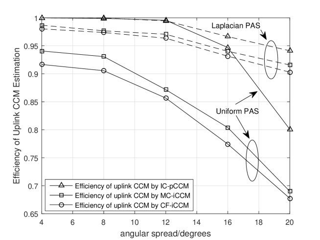
Figure 5: Efficiency of uplink CCMs reconstructed by three methods, with $\nu=16$ and SNR = $10$ dB.

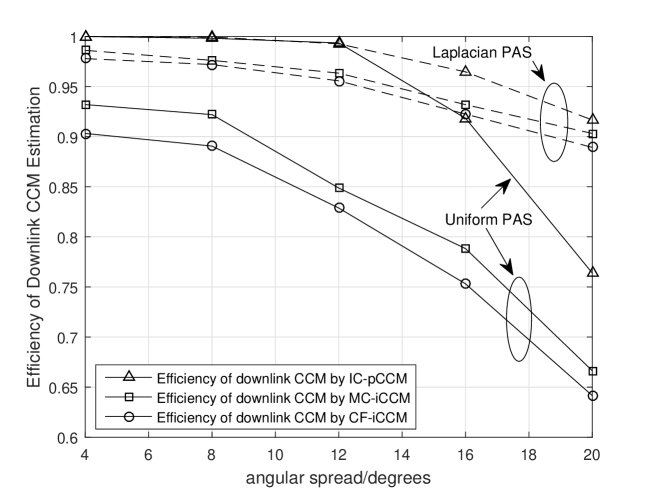
Figure 6: Efficiency of downlink CCMs reconstructed by three methods, with $\nu=16$ and SNR = $10$ dB.

In the first examples, we examine the efficiency of uplink/downlink CCMs reconstruction, defined as

$$\eta\triangleq\frac{1}{N}\sum_{n=1}^{N}\frac{\langle\mathbf{R}_{k,p}(n),\hat{\mathbf{B}}_{k,p}\hat{\mathbf{B}}_{k,p}^{H}\rangle}{\text{tr}\left\{\mathbf{R}_{k,p}(n)\right\}}=\frac{1}{N}\sum_{n=1}^{N}\frac{\text{tr}\{\hat{\mathbf{B}}_{k,p}^{H}\mathbf{R}_{k,p}(n)\hat{\mathbf{B}}_{k,p}\}}{\text{tr}\left\{\mathbf{R}_{k,p}(n)\right\}},$$ (50)

where $\mathbf{R}_{k,p}(n)$ denotes the real CCMs of user-$k$, namely, $\mathbf{R}_{k,p}^{u}(n)$ or $\mathbf{R}_{k,p}^{d}(n)$, and $\hat{\mathbf{B}}_{k,p}\in\mathbb{C}^{M\times\nu}$ includes the $\nu$ dominant eigenvectors of $\hat{\mathbf{R}}^{u}_{k,p}(n)$ or $\hat{\mathbf{R}}^{d}_{k,p}(n)$ corresponding to the $\nu$ largest eigenvalues. Obviously, for any given $\nu\ll M$, if $\eta\approx 1$, then a significant amount of received signal’s power is captured by a low-dimensional signal subspace, which also serves as an indicator of the “similarity” between estimated signal subspaces and the real ones. Besides the IC-pCCM scheme, the efficiencies of CCMs constructed by CF-iCCM and MC-iCCM methods in section II-B with prior knowledge of PAS distributions are also included in Fig. 5 and Fig. 6. For all the methods, the central AOA and AS parameters are estimated from uplink instantaneous channel estimates and then applied for uplink/downlink CCM reconstructions. Meanwhile, the uplink/downlink training power is set as $\rho_{u}=\rho_{d}=10$ dB and the default cardinality of $\mathcal{Q}_{k,p}$ for each user is set as $\kappa=\nu=16$. It can be seen from Fig. 5 and Fig. 6 that when $\nu=16,M=128$, the IC-pCCM scheme could obtain a relative high efficiency for both uplink/downlink CCM estimation, for both uniform and Laplacian PAS distributions, and for both narrow and wide ASs. This demonstrates the effectiveness of CCM reconstruction from instantaneous channel estimates. Meanwhile, the IC-pCCM scheme outperforms the CF-iCCM and MC-iCCM methods for both uplink and downlink CCMs construction. Especially, the performances of CF-iCCM method deteriorate significantly for larger AS and uniform PAS. This is because the performances of CF-iCCM rely heavily on the accuracy of angle estimation, which unfortunately is often deteriorated when multiple users are scheduled at the same time. By contrast, the IC-pCCM scheme is more robust to the angle estimation error for the reason that the value of $\hat{\alpha}(\vartheta)$ will be small if an estimated $\vartheta$ does not belong to the real AOA interval. Furthermore, if Laplacian PAS is considered, the CCM reconstruction efficiencies of all three methods increase for the reason that more channel power is concentrated in central DOAs.

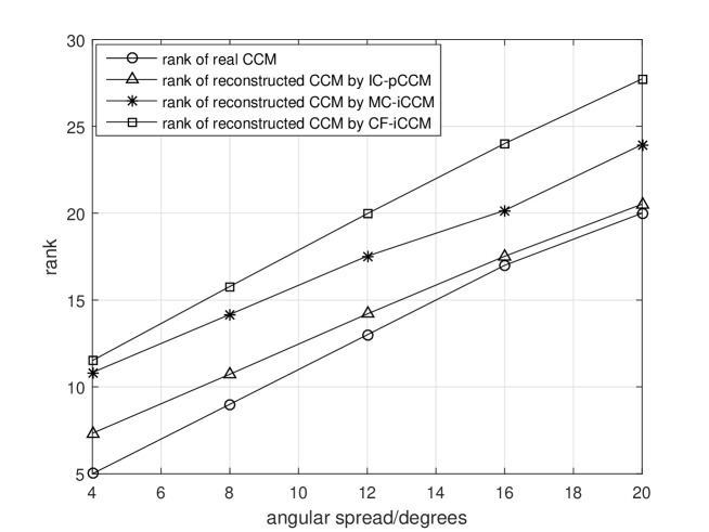
Figure 7: Comparison of Ranks of CCMs reconstructed by different methods, with uniform PAS and SNR=$10$ dB.

Fig. 7 compares the ranks of real uplink CCMs and the estimated uplink CCMs by the three methods as a function of AS with uniform PAS and SNR = $10$ dB. It shows that the ranks of CCMs estimated by IC-pCCM is close to the ranks of real CCMs, while the ranks of CCMs reconstructed by CF-iCCM and MC-iCCM are much larger, which means that a larger angle estimation error will cause a wider spread of the eigenvalues of estimated CCMs by integral methods. Meanwhile, with increasing AS, the gap between ranks of constructed CCMs by CF-iCCM and MC-iCCM also becomes larger. This verifies the discussion in section II-B that MC-iCCM is more accurate than CF-iCCM for large AS.

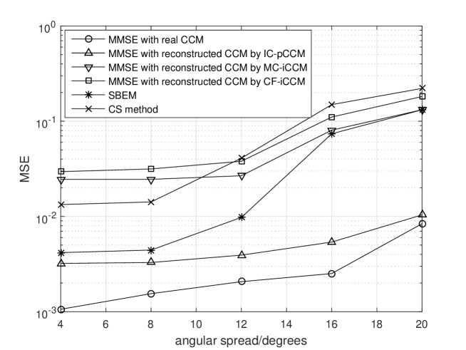
Figure 8: Uplink MSE performances of MMSE estimators with reconstructed CCMs as a function of AS, with $\nu=20$, SNR=$10$ dB and uniform PAS.

Fig. 8 displays the performances of uplink channel estimation via MMSE estimator with CCMs reconstructed by the three different methods. For better comparison, the SBEM [12] and the CS-based method in [9] are also included. The performance metric of the channel estimation is taken as the average individual MSE, i.e.,

$$\text{MSE}\triangleq\frac{1}{NK}\sum_{n=1}^{N}\sum_{k=1}^{K}\frac{\left\|\mathbf{h}_{k,p}(n)-\hat{\mathbf{h}}_{k,p}(n)\right\|^{2}}{\left\|\mathbf{h}_{k,p}(n)\right\|^{2}}.$$

For uplink training, the SNR is set as $\rho_{u}=10$ dB and only $\nu=20$ dominant eigenvectors along with the corresponding eigenvalues are used for uplink channel estimation in (III-B5) for the consideration of limited radio frequency chains and the purpose of training overhead reduction. Fig. 8 illustrates that the MMSE estimator with CCMs reconstructed from uplink channel estimates by IC-pCCM scheme can achieve a significant performance improvement than that of SBEM and only has a small gap between the performance of ideal CCM case. Meanwhile, as AS increases, the performances of SBEM, CF-iCCM, MC-iCCM and CS methods deteriorate greatly, while the MMSE performances with real CCMs and reconstructed CCM via IC-pCCM are relatively more robust to larger ASs. The reason lies in that the eigenvectors of CCMs formulate an optimal set of expansion basis vectors for signal expansion in the logical domain, such that more signal power is accumulated in lower-dimensional signal subspace even in the larger AS conditions. However, the CCMs estimated by CF-iCCM and MC-iCCM methods fail for the inaccurate angle estimation as explained above.

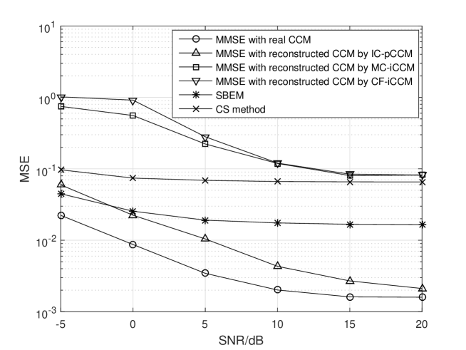
Figure 9: Uplink MSE performances of MMSE estimators with reconstructed CCMs as a function of SNR, with AS $\Delta_{k,p}=10^{\circ}$, $\nu=16$ and uniform PAS.

Fig. 9 then compares the uplink MSE performances of the MMSE estimators with reconstructed CCMs by different methods as well as the SBEM and CS methods as a function of SNR, with AS $\Delta_{k,p}=10^{\circ}$, $\nu=16$ and a uniform PAS. It can be seen that the uplink MSE curves of all methods have their own error floors. There are two main reasons for these error floors. First, only limited number of expansion basis vectors, i.e., $\nu=16$ in Fig. 9, is used for uplink training enhancement in (III-B5). More importantly, the instantaneous channel estimates in (23)-(25) have their own truncation errors by only extracting components of $\hat{\mathbf{h}}_{\mathcal{U}_{1}}(n)$ indexed by $\mathcal{Q}_{k,p}$. This truncation error cannot be improved even by the proposed uplink training enhancement scheme and thus even the MSE curve with real CCM has its own error floor. However, the MSE performance of MMSE with reconstructed CCM by IC-pCCM method has a significant improvement. As explained above, this is because the real CCMs as well as the reconstructed CCMs with IC-pCCM are able to accumulate more power with only $\nu=16$ eigenvectors, which also corroborates the effectiveness and satisfying performance gains provided by IC-pCCM scheme.

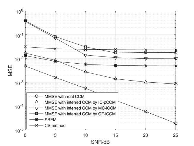
Figure 10: Downlink MSE performances of MMSE estimators with inferred CCMs as a function of SNR, with AS $\Delta_{k,p}=10^{\circ}$, $\nu=20$ and uniform PAS.

Fig. 10 illustrates the downlink MSE performances of the MMSE estimators with inferred CCMs by different methods as well as the SBEM and CS methods as a function of SNR, with AS $\Delta_{k,p}=10^{\circ}$. For donwlink training, only $\nu=20$ dominant eigenvectors along with the corresponding eigenvalues are used for eigen-beamforming in (III-C2) for the same consideration of limited radio frequency chains and reduced training and feedback overhead. It can be seen that the MSE curves of SBEM, CF-iCCM and MC-iCCM methods have their own error floors. Note that different from uplink case, these error floors are only due to the limited number of expansion basis vectors for downlink training. Without truncation error, the MSE curve with real CCM does not have any error floor. Compared to CF-iCCM and MC-iCCM, the MSE performance of MMSE with inferred CCM by IC-pCCM has been improved greatly. Meanwhile, the gap between the MSE performances of CF-iCCM and MC-iCCM methods shows that when AS is large or the narrow AS condition is not satisfied, the CF-iCCM method (6b) using Taylor expansion to approximate (6a) certainly results in performance loss.

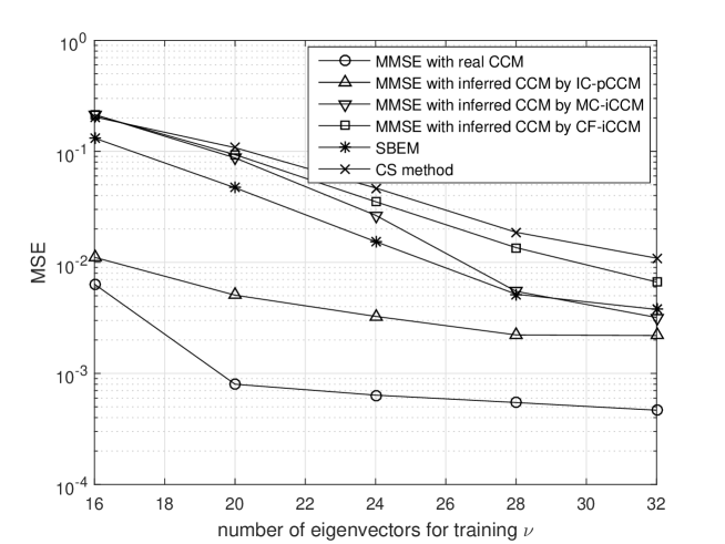
Figure 11: Downlink MSE performances of MMSE estimators with reconstructed CCMs as a function of $\nu$, with AS $\Delta_{k,p}=15^{\circ}$, SNR=$10$ dB and uniform PAS.

As the MSE performances of MMSE estimator with CCMs inferred by different methods are significantly dependent on the value of $\nu$, we illustrate their MSE curves as a function of $\nu$ in Fig. 11. For comparison, the SBEM and CS methods with the same number of training beams are also considered. The downlink SNR is set as 10 dB and the AS is set as $15^{\circ}$. It can be seen that the MSE curves of different methods are going to approach each other as $\nu$ increases. This is intuitively correct as a larger $\nu$ means a higher ratio of the channel power included for training. It is also be seen that the MSE curves of the real CCM and the inferred CCMs by IC-pCCM become flat quickly when $\nu$ is about $20$, while SBEM, CF-iCCM, MC-iCCM and CS methods require $\nu=32$ or larger. Hence, this also indicates the effectiveness of the IC-pCCM scheme for accurate CCM estimation as well as accompanied low overhead channel estimation.

V Conclusions

In this paper, we proposed an enhanced channel estimation scheme for TDD/FDD massive MIMO systems based on uplink/downlink CCMs reconstruction from array signal processing techniques. Specifically, the CCM reconstruction was decomposed into angle estimation and PAS estimation, both of which were extracted from only one instantaneous uplink channel estimate. With estimated angle and PAS, uplink CCMs were first reconstructed and exploited to improve the uplink training performances. Then the downlink CCMs were inferred even in FDD systems. Meanwhile, a dynamical angle division multiple access user scheduling strategy was proposed based on the real-time angle information of users. Compared to existing methods, the proposed method does not need the long-time acquisition for uplink CCMs and could handle a more practical channel propagation environment with larger AS. Moreover, the proposed scheme is applicable for any kind of PAS distributions and array geometries. Numerical simulations have corroborated the effectiveness of our proposed scheme.

References

• [1] T. L. Marzetta, “Noncooperative cellular wireless with unlimited numbers of base station antennas,” IEEE Trans. Wireless Commun., vol. 9, no. 11, pp. 3590–3600, Nov. 2010.
• [2] E. Larsson, O. Edfors, F. Tufvesson, and T. Marzetta, “Massive MIMO for next generation wireless systems,” IEEE Commun. Mag., vol. 52, no. 2, pp. 186–195, Feb. 2014.
• [3] F. Rusek, D. Persson, B. K. Lau, E. G. Larsson, T. L. Marzetta, O. Edfors, and F. Tufvesson, “Scaling up MIMO: Opportunities and challenges with very large arrays,” IEEE Signal Process. Mag., vol. 30, no. 1, pp. 40–60, Jan. 2013.
• [4] C. Sun, X. Gao, S. Jin, M. Matthaiou, Z. Ding, and C. Xiao, “Beam division multiple access transmission for massive MIMO communications,” IEEE Trans. Commun., vol. 63, no. 6, pp. 2170–2184, June 2015.
• [5] H. Yin, D. Gesbert, M. Filippou, and Y. Liu, “A coordinated approach to channel estimation in large-scale multiple-antenna systems,” IEEE J. Sel. Areas Commun., vol. 31, no. 2, pp. 264–273, Feb. 2013.
• [6] A. Adhikary, J. Nam, J.-Y. Ahn, and G. Caire, “Joint spatial division and multiplexing–the large-scale array regime,” IEEE Trans. Inf. Theory, vol. 59, no. 10, pp. 6441–6463, Oct. 2013.
• [7] R. W. Heath, N. Gonz lez-Prelcic, S. Rangan, W. Roh, and A. M. Sayeed, “An overview of signal processing techniques for millimeter wave MIMO systems,” IEEE J. Sel. Topics. Signal Process., vol. 10, no. 3, pp. 436–453, Apr. 2016.
• [8] X. Rao and V. K. Lau, “Distributed compressive CSIT estimation and feedback for FDD multi-user massive MIMO systems,” IEEE Trans. Signal Process., vol. 62, no. 12, pp. 3261–3271, June 2014.
• [9] Z. Gao, L. Dai, Z. Wang, and S. Chen, “Spatially common sparsity based adaptive channel estimation and feedback for FDD massive MIMO,” IEEE Trans. Signal Process., vol. 63, no. 23, pp. 6169–6183, Dec. 2015.
• [10] H. Xie, F. Gao, and S. Jin, “An overview of low-rank channel estimation for massive MIMO systems,” IEEE Access, vol. 4, pp. 7313–7321, Oct. 2016.
• [11] H. Xie, B. Wang, F. Gao, and S. Jin, “A full-space spectrum-sharing strategy for massive MIMO cognitive radio systems,” IEEE J. Sel. Areas. Commun., vol. 34, no. 10, pp. 2537–2549, Oct. 2016.
• [12] H. Xie, F. Gao, S. Zhang, and S. Jin, “A unified transmission strategy for TDD/FDD massive MIMO systems with spatial basis expansion model,” IEEE Trans. Veh. Technol., vol. 66, no. 4, pp. 3170–3184, Apr. 2017.
• [13] R. M ndez-Rial, N. Gonz lez-Prelcic, and R. W. Heath, “Adaptive hybrid precoding and combining in mmwave multiuser MIMO systems based on compressed covariance estimation,” in Proc. IEEE CAMSAP’15, 13–16 Dec. 2015, pp. 213–216.
• [14] S. Haghighatshoar and G. Caire, “Massive MIMO channel subspace estimation from low-dimensional projections,” IEEE Trans. Signal Process., vol. 65, no. 2, pp. 303–318, Jan. 2017.
• [15] K. Hugl, J. Laurila, and E. Bonek, “Downlink beamforming for frequency division duplex systems,” in Proc. IEEE GLOBECOM’99, vol. 4, Rio de Janeireo, Brazil, 1999, pp. 2097–2101.
• [16] Y.-C. Liang and F. P. S. Chin, “Downlink channel covariance matrix (DCCM) estimation and its applications in wireless DS-CDMA systems,” IEEE J. Sel. Areas Commun., vol. 19, no. 2, pp. 222–232, Feb. 2001.
• [17] A. Decurninge, M. Guillaud, and D. T. M. Slock, “Channel covariance estimation in massive mimo frequency division duplex systems,” in Proc. IEEE GLOBECOM’15, San Diego, USA, 6–10 Dec. 2015, pp. 1–6.
• [18] J. Fang, X. Li, H. Li, and F. Gao, “Low-rank covariance-assisted downlink training and channel estimation for FDD massive MIMO systems,” IEEE Trans. Wireless Commun., vol. 16, no. 3, pp. 1935–1947, Mar. 2017.
• [19] D. Vasisht et al., “Eliminating channel feedback in next-generation cellular networks,” in Proc. ACM SIGCOMM, Aug. 2016, pp. 398–411.
• [20] B. Y. Shikur and T. Weber, “Uplink-downlink transformation of the channel transfer function for OFDM systems,” in Proc. InOWo’14, 27-28 Aug. 2014, pp. 1–6.
• [21] D. Tse and P. Viswanath, Fundamentals of wireless communication, Cambridge university press, 2005.
• [22] L. Ye, “Simplified channel estimation for ofdm systems with multiple transmit antennas,” IEEE Trans. Wireless Commun., vol. 1, no. 1, pp. 67–75, Aug. 2002.
• [23] R. Schmidt, “Multiple emitter location and signal parameter estimation,” IEEE Trans. Antennas Propag., vol. 34, no. 3, pp. 276–280, Mar. 1986.
• [24] R. Roy and T. Kailath, “ESPRIT-estimation of signal parameters via rotational invariance techniques,” IEEE Trans. Acoust., Speech, Signal Process., vol. 37, no. 7, pp. 984–995, July 1989.
• [25] J. Fang, J. Li, Y. Shen, H. Li and S. Li, “Super-resolution compressed sensing: An iterative reweighted algorithm for joint parameter learning and sparse signal recovery,” IEEE Signal Process. Lett., vol. 21, no. 6, pp. 761–765, June 2014.
• [26] J. Fang, F. Wang, Y. Shen, H. Li, and R. S. Blum, “Super-resolution compressed sensing for line spectral estimation: An iterative reweighted approach,” IEEE Trans. Signal Process., vol. 64, no. 18, pp. 4649–4662, Sept. 2016.
• [27] K. Pedersen, P. Mogensen, and B. Fleury, “Power azimuth spectrum in outdoor environments,” Electron. Lett., vol. 33, no. 18, pp. 1583–1584, Aug. 1997.
• [28] G. Xu and H. Liu, “An efficient transmission beamforming scheme for frequency-division-duplex digital wireless communications systems,” in Proc. ICASSP’95, 1995, pp. 1729–1732.
• [29] A. Kuchar, M. Tangemann and E. Bonek, “A real-time DOA-based smart antenna processor,” IEEE Trans. Veh. Technol., vol. 51, no. 6, pp. 1279–1293, Nov. 2002.
• [30] S. Imtiaz, G. S. Dahman, F. Rusek, and F. Tufvesson, “On the directional reciprocity of uplink and downlink channels in frequency division duplex systems,” in Proc. IEEE PIMRC, 2015, pp.172–176.
• [31] K. Hugl, K. Kalliola and J. Laurila, “Spatial reciprocity of uplink and downlink radio channels in FDD systems,” in COST 273 TD(02)066, 2002.
• [32] J. M. Goldberg and J. R. Fonollosa, “Downlink beamforming for spatially distributed sources in cellular mobile communications,” Signal Process., vol. 65, pp. 181–197, 1998.
• [33] RI-100053, “On channel reciprocity for enhanced downlink multi-antenna transmission”, Ericsson
• [34] P. Stoica and A. Nehorai, “Music, maximum likelihood, and cramer-rao bound: Further results and comparisons,” IEEE Trans. Acoust., Speech, Signal Processing, vol. 38, no. 12, pp. 2140–2150, Dec. 1990.
• [35] A. M. Sayeed, “Deconstructing multiantenna fading channels” IEEE Trans. Signal Process., vol. 50, no. 10, pp. 2563–2579, Oct. 2002.
• [36] A. Alkhateeb, O. E. Ayach, G. Leus, and R. W. Heath, “Channel estimation and hybrid precoding for millimeter wave cellular systems,” IEEE J. Sel. Topics. Signal Process., vol. 8, no. 5, pp. 831–846, Oct. 2014.