Volumes and Ehrhart polynomials of flow polytopes

Abstract.

The Lidskii formula for the type $A_{n}$ root system expresses the volume and Ehrhart polynomial of the flow polytope of the complete graph with nonnegative integer netflows in terms of Kostant partition functions. For every integer polytope the volume is the leading coefficient of the Ehrhart polynomial. The beauty of the Lidskii formula is the revelation that for these polytopes their Ehrhart polynomial function can be deduced from their volume function! Baldoni and Vergne generalized Lidskii’s result for flow polytopes of arbitrary graphs $G$ and nonnegative integer netflows. While their formulas are combinatorial in nature, their proofs are based on residue computations. In this paper we construct canonical polytopal subdivisions of flow polytopes which we use to prove the Baldoni–Vergne–Lidskii formulas. In contrast with the original computational proof of these formulas, our proof reveal their geometry and combinatorics. We conclude by exhibiting enumerative properties of the Lidskii formulas via our canonical polytopal subdivisions.

Dedicated to the memory of Bertram Kostant

1. Introduction

Flow polytopes are a well studied [1, 2, 9] and rich family of polytopes that include the Pitman–Stanley polytope [21], the Chan–Robbins–Yuen polytope [7] and the Tesler polytope [16]; see [5, 8, 18] for more examples. Flow polytopes have been shown to have close connections with representation theory [1], diagonal harmonics [16] and Schubert polynomials [19], among others. Two fundamental questions about any integer polytope $\mathcal{P}$, including flow polytopes, are: What is the volume of $\mathcal{P}$? What is the Ehrhart polynomial of $\mathcal{P}$?

This paper is concerned with the answers to these question for the case of flow polytopes $\mathcal{F}_{G}({\bf a})$ (defined in Section 2). These questions were answered by Lidskii [13] for $\mathcal{F}_{k_{n+1}}({\bf a})$, where $k_{n+1}$ denotes the complete graph with $n+1$ vertices, and by Baldoni and Vergne [1] for $\mathcal{F}_{G}({\bf a})$, for arbitrary graphs $G$. The Baldoni–Vergne proof relies on residue computations, leaving the combinatorial nature of their formulas a mystery. In this paper we demystify their beautiful formulas appearing in Theorem 1.1 below, by proving them via polytopal subdivisions of $\mathcal{F}_{G}({\bf a})$. We then use the aforementioned polytopal subdivisions to establish enumerative properties of the Baldoni–Vergne–Lidskii formulas. For the notation used in Theorem 1.1 consult Section 2.

Theorem 1.1 (Baldoni–Vergne–Lidskii formulas [1, Thm. 38]).

Let $G$ be a connected graph on the vertex set $[n+1]$, with $m$ edges directed $i\to j$ if $i<j$, with at least one outgoing edge at vertex $i$ for $i=1,\ldots,n$, and let ${\bf a}=(a_{1},\ldots,a_{n},-\sum_{i=1}^{n}a_{i})$, $a_{i}\in\mathbb{Z}_{\geq 0}$. Then

(1.1) $${\rm vol}\mathcal{F}_{G}({\bf a}) =\sum_{{\bf j}}\binom{m-n}{j_{1},\ldots,j_{n}}a_{1}^{j_{1}}\cdots a_{n}^{j_{n}}\cdot K_{G}\left(j_{1}-{\rm out}_{1},\ldots,j_{n}-{\rm out}_{n},0\right),$$

(1.2) $$K_{G}({\bf a}) =\sum_{{{\bf j}}}\binom{a_{1}+{\rm out}_{1}}{j_{1}}\cdots\binom{a_{n}+{\rm out}_{n}}{j_{n}}\cdot K_{G}\left(j_{1}-{\rm out}_{1},\ldots,j_{n}-{\rm out}_{n},0\right),$$

(1.3) $$=\sum_{{{\bf j}}}\mathchoice{\left(\kern-5.0pt{\binom{a_{1}-{\rm in}_{1}}{j_{1}}}\kern-5.0pt\right)}{\bigl{(}\kern-3.00003pt{\binom{a_{1}-{\rm in}_{1}}{j_{1}}}\kern-3.00003pt\bigr{)}}{\bigl{(}\kern-3.00003pt{\binom{a_{1}-{\rm in}_{1}}{j_{1}}}\kern-3.00003pt\bigr{)}}{\bigl{(}\kern-3.00003pt{\binom{a_{1}-{\rm in}_{1}}{j_{1}}}\kern-3.00003pt\bigr{)}}\cdots\mathchoice{\left(\kern-5.0pt{\binom{a_{n}-{\rm in}_{n}}{j_{n}}}\kern-5.0pt\right)}{\bigl{(}\kern-3.00003pt{\binom{a_{n}-{\rm in}_{n}}{j_{n}}}\kern-3.00003pt\bigr{)}}{\bigl{(}\kern-3.00003pt{\binom{a_{n}-{\rm in}_{n}}{j_{n}}}\kern-3.00003pt\bigr{)}}{\bigl{(}\kern-3.00003pt{\binom{a_{n}-{\rm in}_{n}}{j_{n}}}\kern-3.00003pt\bigr{)}}\cdot K_{G}\left(j_{1}-{\rm out}_{1},\ldots,j_{n}-{\rm out}_{n},0\right),$$

for ${\rm out}_{i}={\rm outd}_{i}-1$ and ${\rm in}_{i}={\rm ind}_{i}-1$ where ${\rm outd}_{i}$ and ${\rm ind}_{i}$ denote the outdegree and indegree of vertex $i$ in $G$. Each sum is over weak compositions ${\bf j}=(j_{1},j_{2},\ldots,j_{n})$ of $m-n$ that are $\geq({\rm out}_{1},\ldots,{\rm out}_{n})$ in dominance order and $\mathchoice{\left(\kern-5.0pt{\binom{n}{k}}\kern-5.0pt\right)}{\bigl{(}\kern-3.00003pt{\binom{n}{k}}\kern-3.00003pt\bigr{)}}{\bigl{(}\kern-3.00003pt{\binom{n}{k}}\kern-3.00003pt\bigr{)}}{\bigl{(}\kern-3.00003pt{\binom{n}{k}}\kern-3.00003pt\bigr{)}}:=\binom{n+k-1}{k}$.

In (1.2) $K_{G}({\bf a})$ denotes the Kostant partition function of the graph $G$, which equals the number of lattice points of $\mathcal{F}_{G}({\bf a})$, as explained in Section 2. The Ehrhart function of an integer polytope $\mathcal{P}$ counts the number of lattice points of the dilated polytope $t\mathcal{P}$, and it is a polynomial in $t$. The coefficient of the highest degree term of the Ehrhart polynomial gives the volume of the polytope. The magic of the Baldoni–Vergne–Lidskii formulas is that for flow polytopes $\mathcal{F}_{G}({\bf a})$, their Ehrhart polynomial $K_{G}(t{\bf a})$ can be deduced from their volume function!

The dominance order characterization of the compositions j in Theorem 1.1 is due to Postnikov and Stanley [24]. Postnikov and Stanley also observed that a proof of (1.2) can be obtained via the judicious use of the Elliott–MacMahon algorithm [24]. We use subdivisions of flow polytopes to prove Theorem 1.1, explaining the summands in the RHS of (1.1) and (1.2) geometrically: each composition j encodes a type of cell of the subdivision, the Kostant partition function encodes the number of times that type of cell appears in the subdivision, the rest of the summand corresponds to the volume or lattice point contribution of that type of cell (see Figure 1). To complete our polytopal proof of (1.2), we also need to invoke the Elliott–MacMahon algorithm, similar to the work of Postnikov and Stanley.

Our subdivisions of flow polytopes $\mathcal{F}_{G}({\bf a})$ generalize the Postnikov–Stanley subdivision of the flow polytope $\mathcal{F}_{G}(1,0,\ldots,0,-1)$ (e.g. see [15, §6]). We refer to our subdivisions as the canonical subdivision of $\mathcal{F}_{G}({\bf a})$. We call the full dimensional polytopes in the canonical subdivisions cells. We say that two cells are of the same type if they are encoded by the same composition ${\bf j}$. In Section 6 (see Theorems 6.2 and 6.6) we derive the following formulas for the number of types of cells and the number of cells of the canonical subdivision of $\mathcal{F}_{G}({\bf a})$.

Theorem 1.2.

Let $G$ be a graph with vertex set $[n+1]$ and ${\bf a}=(a_{1},\ldots,a_{n},-\sum_{i=1}^{n}a_{i})$, $a_{i}\in\mathbb{Z}_{>0}$. The number $N$ of types of cells in the canonical subdivision of $\mathcal{F}_{G}({\bf a})$ is given by the determinant

$$N=\det\left[\binom{{\rm out}_{i+1}+\cdots+{\rm out}_{n}+1}{i-j+1}\right]_{1\leq i,j\leq n-1},$$

and the number $M$ of cells of the canonical subdivision of $\mathcal{F}_{G}({\bf a})$ equals

$$M={\rm vol}\mathcal{F}_{G^{\star}}(1,0,\ldots,0,-1).$$

where $G^{\star}$ is obtained from $G$ by adding a vertex $0$ adjacent to vertices $i=1,2,\ldots,n$ of $G$.

We note that while Theorem 1.1 is stated for outdegrees, there are analogues of (1.1) and (1.2) in terms of indegrees of $G$ obtained by reversing the digraph $G$. We state the volume formula here.

Corollary 1.3.

Let $G$ be a graph on the vertex set $[n+1]$ with $m$ edges directed $i\to j$ if $i<j$, with at least one incoming edge at vertex $i$ for $i=2,\ldots,n+1$, and ${\bf b}=(\sum_{i=1}^{n}b_{i},-b_{1},\ldots,-b_{n-1},-b_{n})$ with $b_{i}\in\mathbb{Z}_{\geq 0}$, for $i=1,\ldots,n$. Then

(1.4) $${\rm vol}\mathcal{F}_{G}({\bf b})=\sum_{{\bf j}}\binom{m-n}{j_{1},\ldots,j_{n}}b_{1}^{j_{1}}\cdots b_{n}^{j_{n}}\cdot K_{G}(0,{\rm in}_{2}-j_{1},\ldots,{\rm in}_{n+1}-j_{n}),$$

where ${\rm in}_{i}={\rm ind}_{i}-1$ and ${\rm ind}_{i}$ is the indegree of vertex $i$ in $G$, and the sum is over weak compositions ${\bf j}=(j_{1},j_{2},\ldots,j_{n})$ of $m-n$ that are $\leq({\rm in}_{2},\ldots,{\rm in}_{n+1})$ in dominance order.

Two important relations between the volume of a flow polytope and the number of lattice points of a related flow polytope can be deduced from the volume formulas (1.1) and (1.4) when we specialize to ${\bf a}=(1,0,\ldots,0,-1)$:

Corollary 1.4 ([1, 21]).

For a graph $G$ on the vertex set $[n+1]$ we have that

(1.5) $${\rm vol}\mathcal{F}_{G}(1,0,\ldots,0,-1) =K_{G}(m-n-{\rm out}_{1},-{\rm out}_{2},\ldots,-{\rm out}_{n},0),$$

(1.6) $$=K_{G}(0,{\rm in}_{2},{\rm in}_{3},\ldots,{\rm in}_{n},-m+n+{\rm in}_{n+1}),$$

where ${\rm out}_{i}={\rm outd}_{i}-1$, ${\rm in}_{i}={\rm ind}_{i}-1$ and ${\rm outd}_{i}$, ${\rm ind}_{i}$ denote the outdegree and indegree of vertex $i$ in $G$.

Thus, this corollary states that the volume of $\mathcal{F}_{G}(1,0,\ldots,0)$ equals the number of integer points in either the polytope $\mathcal{F}_{G}(m-n-{\rm out}_{1},-{\rm out}_{2},\ldots,-{\rm out}_{n},0)$ or $\mathcal{F}_{G}(0,{\rm in}_{2},{\rm in}_{3},\ldots,{\rm in}_{n},m-n-{\rm in}_{n+1})$.

We highlight two families of flow polytopes with known product formulas for their volumes. Such formulas are obtained by applying Theorem 1.1.

I. Pitman-Stanley polytopes: Denote by $\Pi_{n}$ the graph on the vertex set $[n+1]$ and edges

$$E(\Pi_{n}):=\{(i,i+1),(i,n+1)\mid i=1,\ldots,n\}.$$

Baldoni and Vergne [1, §3.6] showed that the polytope $\mathcal{F}_{\Pi_{n}}({\bf a})$ is integrally equivalent to the Pitman–Stanley polytope [21]. They showed the Lidskii formulas in this case correspond exactly to the volume and Ehrhart polynomial formulas in [21] both involving Catalan many terms (in the notation of Theorem 1.2 we have $N=C_{n}:=\frac{1}{n+1}\binom{2n}{n}$). Moreover,

$${\rm vol}\mathcal{F}_{\Pi_{n}}({\bf a})=n!\sum_{\bf j}\frac{a_{1}^{j_{1}}}{j_{1}!}\cdots\frac{a_{n}^{j_{n}}}{j_{n}!},$$

where the sum is over the $C_{n}$ many tuples $(j_{1},\ldots,j_{n})$ satisfying $j_{1}+\cdots+j_{n}=n$ and with partial sums $j_{1}\geq 1,j_{1}+j_{2}\geq 2,\ldots$.

II. The Baldoni-Vergne polytopes: When $G$ is the complete graph $k_{n+1}$ with $n+1$ vertices the polytope $\mathcal{F}_{k_{n+1}}({\bf a})$ was studied by Baldoni–Vergne [1]. For special values of ${\bf a}$ these polytopes have interesting volumes:

• when ${\bf a}=(1,0,\ldots,0,-1)$, the polytope $\mathcal{F}_{k_{n+1}}({\bf a})$ is called the Chan-Robbins-Yuen (CRY) polytope [7]. By (1.6) we obtain

  $${\rm vol}\mathcal{F}_{k_{n+1}}(1,0,\ldots,0,-1)=K_{k_{n+1}}(0,0,1,2,\ldots,n-2,-{\textstyle\binom{n-1}{2}}).$$

  Zeilberger [28] showed that $K_{k_{n+1}}(0,0,1,2,\ldots,n-2,-{\textstyle\binom{n-1}{2}})$ is the product of the first $n-1$ Catalan numbers as conjectured by Chan, Robbins and Yuen [7]:

  (1.7) $${\rm vol}\mathcal{F}_{k_{n+1}}(1,0,\ldots,0,-1)=C_{0}C_{1}\cdots C_{n-2}.$$

• when ${\bf a}=(1,1,\ldots,1,-n)$, the polytope $\mathcal{F}_{k_{n+1}}({\bf a})$ is called the Tesler polytope [16] whose lattice points correspond to Tesler matrices, of interest in diagonal harmonics [10]. Applying (1.1) to this polytope yields

  $${\rm vol}\mathcal{F}_{k_{n+1}}(1,1,\ldots,1,-n)=\sum_{{\bf j}}\binom{\binom{n}{2}}{j_{1},j_{2},\ldots,j_{n}}\cdot K_{k_{n+1}}(j_{1}-n+1,j_{2}-n+2,\ldots,j_{n},0).$$

  By Corollary 6.9, the canonical subdivision of this polytope has $M=\prod_{i=0}^{n-1}C_{i}$ cells. In [16] Rhoades and the authors showed that the volume equals

  (1.8) $${\rm vol}\mathcal{F}_{k_{n+1}}(1,1,\ldots,1,-n)=f^{(n-1,n-2,\ldots,1)}\cdot C_{0}C_{1}\cdots C_{n-1}$$

  where $f^{(n-1,n-2,\ldots,1)}$ is the number of standard Young tableaux of shape $(n-1,n-2,\ldots,1)$.

• when ${\bf a}=(1,1,0,\ldots,0,-2)$, the polytope $\mathcal{F}_{k_{n+1}}({\bf a})$ was studied by Corteel, Kim and the first author [8]. Applying (1.1) to this polytope only the terms with compositions ${\bf j}=(j_{1},\binom{n}{2}-j_{1},0,\ldots,0)$ survive. They then show that the volume equals

  $${\rm vol}\mathcal{F}_{k_{n+1}}(1,1,0,\ldots,0,-2)=2^{\binom{n}{2}-1}C_{0}C_{1}\cdots C_{n-2}.$$

The common theme of the proofs of volumes for the polytopes described in (a), (b) and (c) above is the application of the Lidskii volume formula, followed by variations of the Morris constant term identity [20, Thm. 4.13],[29].

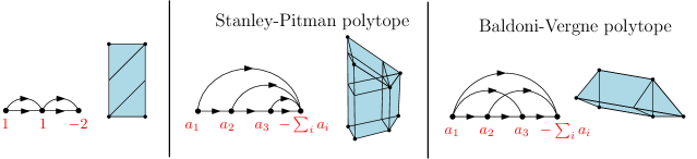
Figure 1. Examples of graphs and their flow polytopes with the canonical subdivision. The second and thid example are instances of the Pitman–Stanley polytope and the Baldoni–Vergne polytope.

Outline

The outline of the paper is as follows. In Section 2 we explain the necessary definitions and background for flow polytopes. In Section 3 we review the subdivision of flow polytopes. In Sections 4 we prove (1.1) via the canonical subdivision, while in Section 5 we prove (1.2). In Section 6 and 7 we study the number of types of cells and the number of cells of subdivisions of flow polytopes with two different techniques: the canonical subdivision and the Cayley trick.

2. Flow polytopes $\mathcal{F}_{G}({\bf a})$ and Kostant partition functions

This section contains the background on flow polytopes and Kostant partition functions, following the exposition of [15]. We also briefly revisit the Pitman–Stanley polytope mentioned in the introduction.

Let $G$ be a (loopless) directed acyclic connected graph on the vertex set $[n+1]$ with $m$ edges. To each edge $(i,j)$, $i<j$, of $G$, associate the positive type $A_{n}$ root $\alpha(i,j)=e_{i}-e_{j}$. Let $S_{G}:=\{\{\alpha(e)\}\}_{e\in E(G)}$ be the multiset of roots corresponding to the multiset of edges of $G$. Let $M_{G}$ be the $(n+1)\times m$ matrix whose columns are the vectors in $S_{G}$. Fix an integer vector ${\bf a}=(a_{1},\ldots,a_{n},-\sum_{i=1}^{n}a_{i})$, $a_{i}\in\mathbb{Z}_{\geq 0}$, referred to as the netflow. An ${\bf a}$-flow ${\bf f}_{G}$ on $G$ is a vector ${\bf f}_{G}=(f(e))_{e\in E(G)}\in\mathbb{R}_{\geq 0}^{|E(G)|}$, such that $M_{G}{\bf f}_{G}={\bf a}$. That is, for all $1\leq i\leq n$, we have

(2.1) $$\sum_{e=(g,i)\in E(G)}f(e)+a_{i}=\sum_{e=(i,j)\in E(G)}f(e)$$

These equations imply that the netflow of vertex $n+1$ is $-\sum_{i=1}^{n}a_{i}$.

Define the flow polytope $\mathcal{F}_{G}({\bf a})$ associated to a graph $G$ on the vertex set $[n+1]$ and the integer netflow vector ${\bf a}$ as the set of all ${\bf a}$-flows ${\bf f}_{G}$ on $G$, i.e., $\mathcal{F}_{G}({\bf a})=\{{\bf f}_{G}\in\mathbb{R}^{m}_{\geq 0}\mid M_{G}{\bf f}_{G}={\bf a})\}$. If ${\bf a}$ is in the cone generated by $S_{G}$ then $\mathcal{F}_{G}({\bf a})$ is not empty and if ${\bf a}$ is in the interior of this cone then $\dim(\mathcal{F}_{G}({\bf a}))=m-n$ [1, §1.1].

The flow polytope $\mathcal{F}_{G}({\bf a})$ can be written as a Minkowski sum of flow polytopes $\mathcal{F}_{G}(e_{i}-e_{n+1})$:

Proposition 2.1 ([1, §3.4]).

For nonnegative integers $a_{1},\ldots,a_{n}$ and $G$ a graph on the vertex set $[n+1]$ we have that

(2.2) $$\mathcal{F}_{G}({\bf a})=a_{1}\mathcal{F}_{G}(e_{1}-e_{n+1})+a_{2}\mathcal{F}_{G}(e_{2}-e_{n+1})+\cdots+a_{n}\mathcal{F}_{G}(e_{n}-e_{n+1}).$$

Proof (sketch).

By adding the flows edge-wise it follows that the Minkowski sum is contained in $\mathcal{F}_{G}({\bf a})$. The other inclusion can be shown by induction on the number of vertices with nonzero netflow $a_{i}$. ∎

The Kostant partition function $K_{G}$ evaluated at the vector ${\bf a}\in\mathbb{Z}^{n+1}$ is defined as

(2.3) $$K_{G}({\bf a})=\#\Big{\{}(f(e))_{e\in E(G)}\Bigm{|}\sum_{e\in E(G)}f(e)\alpha(e)={\bf a}\textrm{ and }f(e)\in\mathbb{Z}_{\geq 0}\Big{\}},$$

where $\{\{\alpha(e)\}\}_{e\in E(G)}$ is the multiset of positive roots corresponding to the multiset of edges of $G$ defined above. In other words, $K_{G}({\bf a})$ is the number of ways to write the vector ${\bf a}=(a_{1},\ldots,a_{n},-\sum_{i=1}^{n}a_{i})$ as a $\mathbb{N}$-linear combination of the positive type $A_{n}$ roots $\alpha(e)$ corresponding to the edges of $G$, without regard to order. Note that $K_{G}({\bf a})$ is the number of lattice points of the flow polytope $\mathcal{F}_{G}({\bf a})$.

The function $K_{G}({\bf a})$ is a piecewise polynomial function in $a_{1},a_{2},\ldots,a_{n}$ (e.g. see [25, Thm. 1.] and [1, Thm. 13]). In fact, for vectors $(a_{1},\ldots,a_{n},-\sum_{i}a_{i})$ in $\mathbb{Z}^{n+1}$ with $a_{i}\geq 0$, the function $K_{G}({\bf a})$ is a polynomial.

Proposition 2.2 ([1, Sec. 2.2]).

For ${\bf a}=(a_{1},\ldots,a_{n},-\sum_{i}a_{i})$ in $\mathbb{Z}^{n+1}$ with $a_{i}\geq 0$ for $i=1,\ldots,n$, the function $K_{G}({\bf a})$ is a polynomial in $a_{1},\ldots,a_{n}$.

The function $K_{G}({\bf a})$ has the following formal generating series:

(2.4) $$\sum_{{\bf a}\in\mathbb{Z}^{n+1}}K_{G}({\bf a})x_{1}^{a_{1}}\cdots x_{n+1}^{-\sum_{i}a_{i}}={\prod_{(i,j)\in E(G)}}(1-x_{i}/x_{j})^{-1},$$

where we order the variables $x_{1}<x_{2}<\ldots<x_{n+1}$ in order for the expansion to be well defined.

By reversing the flow on a graph we obtain the following relation of flow polytopes and the Kostant partition function. Given a directed graph $G$ with vertices $[n+1]$ we denote by $G^{r}$ the graph with vertices $[n+1]$ and edge $E(G^{r})=\{(i,j)\mid(n+2-j,n+2-i)\in E(G)\}$. That is, the graph obtained from $G$ by reversing the edges and relabeling the vertices $i\mapsto n+1-i$. We say that two polytopes $P\subset\mathbb{R}^{n_{1}}$, $Q\subset\mathbb{R}^{n_{2}}$ are integrally equivalent if there is an affine transformation $\varphi:\mathbb{R}^{n_{1}}\to\mathbb{R}^{n_{2}}$ that restricts to a bijection between $P$ and $Q$ and between $\operatorname{aff}(P_{1})\cap\mathbb{Z}^{n_{1}}$ and $\operatorname{aff}(Q)\cap\mathbb{Z}^{n_{2}}$. Integrally equivalent polytopes have the same face lattice, volume, and Ehrhart polynomials. We denote this equivalence by $P\equiv Q$.

Proposition 2.3.

For a graph $G$ on the vertex set $[n+1]$ and $(a_{1},\ldots,a_{n})\in\mathbb{Z}^{n}$:

$$\mathcal{F}_{G}(a_{1},\ldots,a_{n},-{\textstyle\sum_{i=1}^{n}a_{i}})\equiv\mathcal{F}_{G^{r}}({\textstyle\sum_{i=1}^{n}a_{i}},-a_{n},\ldots,-a_{1}).$$

Proof.

Given an ${\bf a}$-flow ${\bf f}_{G}=(f_{e})_{e\in E(G)}$, let ${\bf f}_{G^{r}}=(f^{\prime}(e))_{e\in E(G^{r})}$ be the flow defined by $f^{\prime}(i,j)=f(n+2-j,n+2-i)$. Note that ${\bf f}_{G^{r}}$ is a ${\bf a}^{r}$-flow where ${\bf a}^{r}=(\sum_{i=1}^{n}a_{i},-a_{n},\ldots,-a_{1})$. The map ${\bf f}_{G}\mapsto{\bf f}^{\prime}_{G^{r}}$ is reversible and defines a correspondence between the ${\bf a}$-flows and ${\bf a}^{r}$-flows. ∎

If we restrict to counting integer points in the two integrally equivalent polytopes in Proposition 2.3, we obtain the following identity of Kostant partition functions:

Corollary 2.4.

For a graph $G$ on the vertex set $[n+1]$ and $(a_{1},\ldots,a_{n})\in\mathbb{Z}^{n}$:

$$K_{G}(a_{1},\ldots,a_{n},-{\textstyle\sum_{i=1}^{n}a_{i}})=K_{G^{r}}({\textstyle\sum_{i=1}^{n}a_{i}},-a_{n},\ldots,-a_{1}).$$

We end our background on flow polytopes by giving a characterization of the vertices of $\mathcal{F}_{G}({\bf a})$.

Proposition 2.5 ([11, Lemma 2.1]).

The vertices of $\mathcal{F}_{G}({\bf a})$ are characterized as ${\bf a}$-flows whose support yields a subgraph of $G$ with no (undirected) cycles.

As we will see, the flow polytope $\mathcal{F}_{G}(e_{1}-e_{n+1})$ is of particular interest. Their vertices are particularly easy to describe. Given a path ${\sf p}$ in $G$ from vertex $1$ to vertex $n+1$, let ${\bf f}({\sf p})$ be the unit flow with support in ${\sf p}$.

Corollary 2.6 ([9, Cor. 3.1]).

The vertices of $\mathcal{F}_{G}(e_{1}-e_{n+1})$ are the unit flows ${\bf f}({\sf p})$ where ${\sf p}$ is a path in $G$ from vertex $1$ to vertex $n+1$.

We now sketch the proof that the Pitman–Stanley polytope (mentioned in the introduction) is a flow polytope. Recall that the Pitman–Stanley polytope is

$$\operatorname{PS}(a_{1},\ldots,a_{n}):=\{(x_{1},\ldots,x_{n})\in\mathbb{R}^{n}\mid x_{i}\geq 0,x_{1}+\cdots+x_{i}\leq a_{1}+\cdots+a_{i}\text{ for }i=1,\ldots,n\},$$

for parameters $a_{1},\ldots,a_{n}$ with $a_{i}\geq 0$. This polytope was defined and studied in [21] and it is an important example of a generalized permutahedron [22]. In [3, Ex. 16], Baldoni and Vergne showed that this polytope is integrally equivalent to the flow polytope $\mathcal{F}_{\Pi_{n}}({\bf a})$ defined in the introduction:

Proposition 2.7 ([3]).

The polytopes $\mathcal{F}_{\Pi_{n}}(a_{1},\ldots,a_{n},-\sum_{i}a_{i})$ and $\operatorname{PS}(a_{1},\ldots,a_{n})$ are integrally equivalent.

Proof (sketch).

The affine transformation $\varphi$ between the polytopes $\operatorname{PS}(a_{1},\ldots,a_{n})$ and $\mathcal{F}_{\Pi_{n}}({\bf a})$ is defined as follows $\varphi:(x_{1},\ldots,x_{n})\mapsto{\bf f}_{\Pi_{n}}$ where

$$f(i,j)=\begin{cases}x_{i}&\text{ if }j=n+1,\\ (a_{1}+\cdots+a_{i})-(x_{1}+\cdots+x_{i})&\text{ if }j=i+1.\end{cases}$$

∎

We note that when the parameters $a_{i}$ are positive integers the number of lattice points of $\operatorname{PS}(a_{1},\ldots,a_{n})$ counts certain plane partitions and is given by a determinant.

Theorem 2.8 ([21, Thm. 12]).

For $(a_{1},\ldots,a_{n})\in\mathbb{N}^{n}$, the number of lattice points of the Pitman–Stanley polytope $PS(a_{1},\ldots,a_{n})$ equals the number of plane partitions of shape $(a_{1},a_{1}+a_{2},\ldots,\sum_{i=1}^{n}a_{i})$ with largest parts at most $2$. This number is given by the determinant

$$\#(\operatorname{PS}(a_{1},\ldots,a_{n})\cap\mathbb{Z}^{n})=\det\left[\binom{a_{1}+\cdots+a_{n-i+1}+1}{i-j+1}\right]_{1\leq i,j\leq n}.$$

3. Subdividing flow polytopes

This section explains our method of subdividing flow polytopes. We explain basic and compounded reduction rules (Sections 3.1 and 3.2 respectively), and characterize the polytopes obtained in a subdivision of $\mathcal{F}_{G}({\bf a})$ via these rules (Section 3.3).

3.1. Basic subdivision of flow polytopes

Given a graph $G$ on the vertex set $[n+1]$ and $(a,i),(i,b)\in E(G)$ for some $a<i<b$, let $G_{1}$ and $G_{2}$ be graphs on the vertex set $[n+1]$ with edge sets

$$E(G_{1}) =E(G)\backslash\{(i,b)\}\cup\{(a,b)\},$$

$$E(G_{2}) =E(G)\backslash\{(a,i)\}\cup\{(a,b)\}.$$

We refer to replacing $G$ by $G_{1}$ and $G_{2}$ as above as the basic reduction, or BR for short; see Figure 2. The main result regarding the basic reduction is as follows:

(BR)

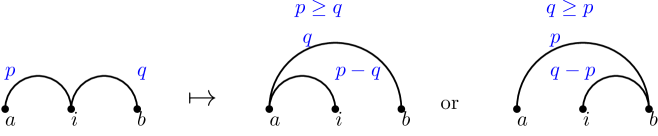
Figure 2. Basic reduction rule (BR). The original edges have flow $p$ and $q$. The outcomes have reassigned flows to preserve the original netflow on the vertices.

Proposition 3.1 (Basic subdivision lemma).

Given a graph $G$ on the vertex set $[n+1]$, ${\bf a}\in\mathbb{Z}^{n}$, and two edges $e_{1}$ and $e_{2}$ of $G$ on which the basic reduction (BR) can be performed yielding the graphs $G_{1},G_{2}$, then

$$\mathcal{F}_{G}({\bf a})=\mathcal{P}_{1}\bigcup\mathcal{P}_{2}\quad\text{ and }\quad\mathcal{P}_{1}^{\circ}\bigcap\mathcal{P}_{2}^{\circ}=\varnothing,$$

where $\mathcal{P}_{i}$ is integrally equivalent to $\mathcal{F}_{G_{i}}({\bf a})$, $i\in[2]$, and $\mathcal{P}^{\circ}$ denotes the interior of $\mathcal{P}$.

The proof of Proposition 3.1 is left to the reader. See [15, 19] for proofs of this lemma. Remark 3.3 expands more on the integral equivalence; by abuse of notation we will generally refer to $\mathcal{P}_{i}$ in Proposition 3.1 as $\mathcal{F}_{G_{i}}({\bf a})$, for $i=1,2$.

We can encode a series of basic reductions on a flow polytope $\mathcal{F}_{G}({\bf a})$ in a rooted tree called the basic reduction tree, or BRT for short; see Figure 6 for an example. The root of this tree is the original graph $G$. After doing a BR on the edges $(a,i),(i,b)$, $a<i<b$, the descendant nodes of the root are the graphs $G_{1},G_{2}$ as above. For each new node we repeat this process to define its descendants. If a node of this tree has a graph $H$ with no edges $(a,i),(i,b)$, $a<i<b$, then the node is a leaf of the BRT.

3.2. Compounded subdivision of flow polytopes

Repeated use of the basic subdivision lemma (Proposition 3.1) yields the canonical subdivision of flow polytopes as we explain in Section 4. In this section we state the compounded subdivision lemma (Proposition 3.4), which is the result of applying the basic reduction rules repeatedly on the incoming and outgoing edges of a fixed vertex of $G$. The compounded subdivision lemma is a refinement of the subdivision lemma given in [15, §5]. To state the result we introduce the necessary notation following [15].

A bipartite noncrossing tree is a tree with a distinguished bipartition of vertices into left vertices $x_{1},\ldots,x_{\ell}$ and right vertices $x_{\ell+1},\ldots,x_{\ell+r}$ with no pair of edges $(x_{p},x_{\ell+q}),(x_{t},x_{\ell+u})$ where $p<t$ and $q>u$. Denote by $\mathcal{T}_{L,R}$ the set of bipartite noncrossing trees where $L$ and $R$ are the ordered sets $(x_{1},\ldots,x_{\ell})$ and $(x_{\ell+1},\ldots,x_{\ell+r})$ respectively. Note that $\#\mathcal{T}_{L,R}=\binom{\ell+r-2}{\ell-1}$, since they are in bijection with weak compositions of $r-1$ into $\ell$ parts. Namely, a tree $T$ in $\mathcal{T}_{L,R}$ corresponds to the composition $(b_{1},\ldots,b_{\ell})$ of $r-1$, where $b_{i}$ denotes the number of edges incident to the left vertex $x_{\ell+i}$ in $T$ minus $1$.

Example 3.2.

The bipartite noncrossing tree encoded by the composition $(0,2,1,1)$ is the following:

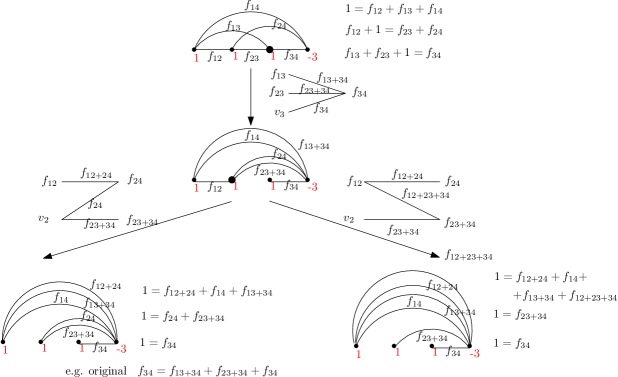
Figure 3. Compounded reduction tree with change of variables indicated (see Remark 3.3). The vertex of the graph where the compounded reduction is taking place is enlarged. The flow polytopes corresponding to the leaves of the compounded reduction tree (CRT) subdivide the flow polytope corresponding to the root of the tree. Compare to the basic reduction tree of the same graph in Figure 6.

Consider a graph $G$ on the vertex set $[n+1]$ and an integer netflow vector ${\bf a}=(a_{1},\ldots,a_{n},-\sum_{i}a_{i})$. Pick an arbitrary vertex $i$,$1<i<n+1$, of $G$. There are two cases depending on whether $a_{i}=0$ or $a_{i}>0$.

• Case 1: $a_{i}=0$. Given a graph $G$ and one of its vertices $i$, let $\mathcal{I}_{i}=\mathcal{I}_{i}(G)$ be the multiset of incoming edges to $i$, which are defined as edges of the form $(\cdot,i)$. Let $\mathcal{O}_{i}=\mathcal{O}_{i}(G)$ be the multiset of outgoing edges from $i$, which are defined as edges of the form $(i,\cdot)$. Define ${\rm ind}_{G}(i):=\#\mathcal{I}_{i}(G)$ to be the indegree of vertex $i$ in $G$.

  Assign an ordering to the sets $\mathcal{I}_{i}$ and $\mathcal{O}_{i}$ and consider a tree $T\in\mathcal{T}_{\mathcal{I}_{i},\mathcal{O}_{i}}$. For each tree-edge $(e_{1},e_{2})$ of $T$ where $e_{1}=(r,i)\in\mathcal{I}_{i}$ and $e_{2}=(i,s)\in\mathcal{O}_{i}$ let $edge(e_{1},e_{2})=(r,s)$. We think of $edge(e_{1},e_{2})$ as a formal sum of the edges $e_{1}$ and $e_{2}$.

  The graph $G^{(i)}_{T}$ is then defined as the graph obtained from $G$ by deleting all edges in $\mathcal{I}_{i}\cup\mathcal{O}_{i}$ of $G$ and adding the multiset of edges $\{\{edge(e_{1},e_{2})~{}|~{}(e_{1},e_{2})\in E(T)\}\}$, and edge $(i,n+1)$.

• Case 2: $a_{i}>0$. Instead of considering $T\in\mathcal{T}_{\mathcal{I}_{i},\mathcal{O}_{i}}$ we consider $T\in\mathcal{T}_{\mathcal{I}_{i}\cup\{i\},\mathcal{O}_{i}}$. The edges of $T$ are as in the previous case, with the exception that $edge(i,(i,j))=(i,j)$. We define $G^{(i)}_{T}$ as the graph obtained from $G$ by deleting all edges in $\mathcal{I}_{i}\cup\mathcal{O}_{i}$ of $G$ and adding the multiset of edges of $T$.

Note that in both cases, the graph $G^{(i)}_{T}$ has no incoming edges to vertex $i$. See Figure 3.

Remark 3.3.

We make the following precision when we refer to $\mathcal{F}_{G_{T}^{(i)}}({\bf a})$. Each edge of $G^{(i)}_{T}$ is a sum of (one or more) edges of the original graph $G$. As mentioned in Proposition 2.5, the vertices of $\mathcal{F}_{G_{T}^{(i)}}({\bf a})$ are given by ${\bf a}$-flows on acyclic subgraphs of ${G_{T}^{(i)}}$. The acyclic subgraphs of ${G_{T}^{(i)}}$ can be mapped to acyclic subgraphs of $G$ by mapping each edge $e$ of the acyclic subgraph of ${G_{T}^{(i)}}$ to the edges in $G$ that are formal summands of $e$. Moreover, with the previous map the ${\bf a}$-flows on acyclic subgraphs of ${G_{T}^{(i)}}$ then map to ${\bf a}$-flows on acyclic subgraphs of $G$. By abuse of notation when we refer to the flows in $\mathcal{F}_{G_{T}^{(i)}}({\bf a})$ we interpret them in the context of $G$. Thus we define $\mathcal{F}_{G_{T}^{(i)}}({\bf a})$ as the convex hull of the ${\bf a}$-flows we obtain on $G$ as above. We do this so that $\mathcal{F}_{G_{T}^{(i)}}({\bf a})\subseteq\mathcal{F}_{G}({\bf a})$.

The proof of Theorem 1.1 relies on the following lemma.

Lemma 3.4 (Compounded subdivision lemma).

Let $G$ be a graph on the vertex set $[n+1]$. Fix an integer netflow vector ${\bf a}=(a_{1},\ldots,a_{n},-\sum_{i=1}^{n}a_{i})$, $a_{i}\in\mathbb{Z}_{\geq 0}$ and a vertex $i\in\{2,\ldots,n\}$ with incoming edges. Then,

(3.1) $$\mathcal{F}_{G}({\bf a})=\bigcup_{T\in\mathcal{T}_{L,R}}\mathcal{F}_{G_{T}^{(i)}}({\bf a}),$$

where

(3.2) $$\mathcal{T}_{L,R}=\begin{cases}\mathcal{T}_{\mathcal{I}_{i},\mathcal{O}_{i}}&\text{ if }a_{i}=0,\\ \mathcal{T}_{\mathcal{I}_{i}\cup\{i\},\mathcal{O}_{i}}&\text{ if }a_{i}>0.\end{cases}$$

Moreover, $\{\mathcal{F}_{G_{T}^{(i)}}({\bf a})\}_{T\in\mathcal{T}_{L,R}}$ are interior disjoint and of the same dimension as $\mathcal{F}_{G}({\bf a})$.

Proof.

The case $a_{i}=0$ is proved in [15, Lemma 5.4] where in our setup $G_{T}^{(i)}$ has an edge $(i,n+1)$ with zero flow since $a_{i}=0$. Next, we prove the case $a_{i}>0$.

Let $\widehat{G}$ be the graph obtained from $G$ by adding vertex $0$ and the edge $(0,i)$ and

$$\hat{{\bf a}}:=(a_{i},a_{1},\ldots,a_{i-1},0,a_{i+1},\ldots,a_{n},-{\textstyle\sum_{i}a_{i}}).$$

The flow polytopes $\mathcal{F}_{G}({\bf a})$ and $\mathcal{F}_{\widehat{G}}(\hat{{\bf a}})$ integrally equivalent. This follows since any $\hat{{\bf a}}$-flow on $\mathcal{F}_{\widehat{G}}(\hat{{\bf a}})$ has flow $a_{i}$ on the edge $(0,i)$. Thus, restricting any $\hat{{\bf a}}$-flow on $\mathcal{F}_{\widehat{G}}(\hat{{\bf a}})$ to the edges of $G$ gives a flow in $\mathcal{F}_{G}({\bf a})$. By applying the subdivision lemma proved in [15, Lemma 5.4] to $\mathcal{F}_{\widehat{G}}(\hat{a})$ on vertex $i$ with zero flow we obtain

$$\mathcal{F}_{\widehat{G}}(\hat{{\bf a}})=\bigcup_{T\in\mathcal{T}_{\hat{L},R}}\mathcal{F}_{\widehat{G}_{T}^{(i)}}(\hat{{\bf a}}).$$

where $\hat{L}=\mathcal{I}_{i}(G)\cup\{v_{0}\}$, $R=\mathcal{O}_{i}(G)$ and $\{\mathcal{F}_{\widehat{G}_{T}^{(i)}}(\hat{{\bf a}})\}_{T\in\mathcal{T}_{L\cup\{v_{0}\},R}}$ are interior disjoint and of the same dimension as $\mathcal{F}_{\widehat{G}}(\hat{{\bf a}})$. Bipartite noncrossing trees $T$ in $\mathcal{T}_{\mathcal{I}_{i}\cup\{v_{0}\},\mathcal{O}_{i}}$ are in correspondence with trees $T^{\prime}$ in $\mathcal{T}_{\mathcal{I}_{i}\cup\{v_{i}\},\mathcal{O}_{i}}$ by relabeling vertex $v_{0}$ to $v_{i}$. Next, by identifying edges $edge((0,i),(i,j))$ (and their flows) in $\widehat{G}^{(i)}_{T}$ (in $\mathcal{F}_{\widehat{G}^{(i)}_{T}}(\hat{{\bf a}})$) with edges $edge(v_{i},(i,j))$ (and their flows) in $G^{(i)}_{T}$ (in $\mathcal{F}_{G_{T}^{(i)}}({\bf a})$) we see that the $\mathcal{F}_{\widehat{G}^{(i)}_{T}}(\hat{{\bf a}})\equiv\mathcal{F}_{G_{T}^{(i)}}({\bf a})$ and

$$\mathcal{F}_{G}({\bf a})=\bigcup_{T\in\mathcal{T}_{\mathcal{I}_{i}\cup\{v_{i}\},\mathcal{O}_{i}}}\mathcal{F}_{G_{T}^{(i)}}({\bf a}),$$

and the polytopes $\mathcal{F}_{G^{(i)}_{T}}({\bf a})$ (interpreted as in Remark 3.3) are interior disjoint and of the same dimension as $\mathcal{F}_{G}({\bf a})$. ∎

We refer to replacing $G$ by $\{G_{T}^{(i)}\}_{T\in\mathcal{T}_{L,R}}$ as in Lemma 3.4 as a compounded reduction, or CR for short. We can encode a series of compounded reductions on a flow polytope $\mathcal{F}_{G}({\bf a})$ in a rooted tree called the compounded reduction tree, or CRT for short; see Figure 3 for an example. The root of this tree is the original graph $G$. After doing reductions on vertex $i$, the descendant nodes of the root are the graphs $\mathcal{F}_{G^{(i)}_{T}}({\bf a})$ from the lemma. For each new node we repeat this process to define its descendants. If a node of this tree has a graph $H$ with no vertices $i=2,\ldots,n$ with both incoming and outgoing edges, then the node is a leaf of the reduction tree. Note that the flow polytopes $\mathcal{F}_{H}({\bf a})$ of the graphs $H$ at the leaves of the tree have the same dimension as $\mathcal{F}_{G}({\bf a})$.

Example 3.5.

Figure 3 gives a CRT for the polytope $\mathcal{F}_{k_{4}}(1,1,1,-3)$. The root of the reduction tree is labeled by the complete graph $k_{4}$. Then we apply a compounded reduction at vertex $3$ to obtain the graph $H:=([4],\{(1,2),(1,4),(1,4),(2,4),(2,4),(3,4)\})$. On $H$ we do a CR at vertex $2$ yielding two outcomes $H_{1}$ and $H_{2}$, drawn on the last row of the figure. Note that in both $H_{1}$ and $H_{2}$ there are no vertices with both incoming and outgoing edges. This means we cannot do any more CR on them. Such graphs are the leaves of this CRT. By Lemma 3.4 the flow polytopes corresponding to the leaves of a CRT with root $G$ are a dissection of the flow polytope $\mathcal{F}_{G}({\bf a})$.

3.3. Subdividing $\mathcal{F}_{G}({\bf a})$ into polytopes of known volume

The following lemma describes the leaves of any compounded reduction tree rooted at $G$. Given a tuple ${\bf m}=(m_{1},\ldots,m_{n})$ of positive integers, let $G({\bf m})$ be the graph with vertices $[n+1]$ and $m_{i}$ edges $(i,n+1)$.

Lemma 3.6.

Given the flow polytope $\mathcal{F}_{G}({\bf a})$ with $G$ a graph on the vertex set $[n+1]$ and $a_{i}\geq 0$ for $i\in[n]$, the leaves of any compounded reduction tree $R_{G}$ rooted at $G$ are graphs of the form $G({\bf m})$ with $m_{i}=1$ if and only if $a_{i}=0$ and $\sum_{i=1}^{n}m_{i}=\#E(G).$.

Proof.

The result follows by iterating the compounded subdivision lemma (Lemma 3.4). The leaves of $R_{G}$ will consist of graphs with no incoming edges in vertices $i=2,\ldots,n$ such that their flow polytopes have same dimension as $\mathcal{F}_{G}({\bf a})$. ∎

Remark 3.7.

We at times refer to the leaves described in Lemma 3.6 as the full dimensional leaves of the CRT to emphasize that they yield flow polytopes of the same dimension as the one we started with. This will be in contrast with some of the leaves we obtain in Section 5 in the basic reduction tree.

Example 3.8.

The two leaves of the reduction tree in Figure 3 are the graphs $G(3,2,1)$ and $G(4,1,1)$.

Next we calculate the volume of the polytopes $\mathcal{F}_{G({\bf m})}({\bf a})$.

Lemma 3.9.

Given $G({\bf m})$ on the vertex set $[n+1]$ with ${\bf m}=(m_{1},\ldots,m_{n})$ a tuple of positive integers, ${\bf a}=(a_{1},\ldots,a_{n})\in\mathbb{Z}_{\geq 0}^{n}$, the normalized volume of $\mathcal{F}_{G({\bf m})}({\bf a})$ is

(3.3) $${\rm vol}(\mathcal{F}_{G({\bf m})}({\bf a}))={{\#E(G({\bf m}))-n}\choose{m_{1}-1,\ldots,m_{n}-1}}a_{1}^{m_{1}-1}\cdots a_{n}^{m_{n}-1}.$$

Proof.

The flow polytope $\mathcal{F}_{G({\bf m})}({\bf a})$ has dimension $\#E(G({\bf m}))-n$ and is the product $\prod_{i=1}^{n}a_{i}\Delta_{m_{i}-1}$ of dilated $(m_{i}-1)$-standard simplices $a_{i}\Delta_{m_{i}-1}$ each of which has (standard) volume $a_{i}^{m_{i}-1}/(m_{i}-1)!$ [4, Thm. 2.2]. Thus the normalized volume of $\mathcal{F}_{G({\bf m})}({\bf a})$ is

$${\rm vol}(\mathcal{F}_{G({\bf m})}({\bf a})) =\dim(\mathcal{F}_{G({\bf m})}({\bf a}))!\cdot\prod_{i=1}^{n}\frac{a_{i}^{m_{i}-1}}{(m_{i}-1)!}$$

$$={{\#E(G({\bf m}))-v}\choose{m_{1}-1,\ldots,m_{n}-1}}a_{1}^{m_{1}-1}\cdots a_{v}^{m_{n}-1}.$$

∎

In order to calculate the volume ${\rm vol}(\mathcal{F}_{G}({\bf a}))$ we need to count the number of times leaves of the form $G({\bf m})$ appear in a certain reduction tree $R^{\leftarrow}_{G}$ and sum over all their volumes. We tackle this in the next section.

4. The canonical subdivision of $\mathcal{F}_{G}({\bf a})$
aka proving the Lidskii volume formula

This section is devoted to proving the Lidskii volume formula (1.1). We achieve this by constructing a canonical subdivision of $\mathcal{F}_{G}({\bf a})$ via the compounded subdivision lemma. In the canonical subdivision we know the volume of each of the full dimensional polytopes (Lemma 3.9) – referred to as cells of the subdivision – and we count how many of each of the cells occur in the canonical subdivision.

4.1. The canonical compounded reduction tree

Given $\mathcal{F}_{G}({\bf a})$, ${\bf a}=(a_{1},\ldots,a_{n},-\sum_{i=1}^{n}a_{i})$, $a_{i}\in\mathbb{Z}_{\geq 0}$, let ${R^{\leftarrow}_{G}}$ be the compounded reduction tree obtained by executing the compounded reductions described in the compounded subdivision lemma on vertices $n,n-1,\ldots,2$ of $G$ in this order. We refer to ${R^{\leftarrow}_{G}}$ as the canonical compounded reduction tree of $G$, or CCRT for short. Figure 4 shows an example of one path from $G$ to a full dimensional leaf in ${R}^{\leftarrow}_{G}$.

We refer to the subdivision obtained from the CCRT via the compounded subdivision lemma as the canonical subdivision of $\mathcal{F}_{G}({\bf a})$. See Figure 5 for an example. We note that the compounded subdivision lemma implies that the canonical subdivision is a dissection; the results of [17, Section 6] imply that it is also a subdivision.

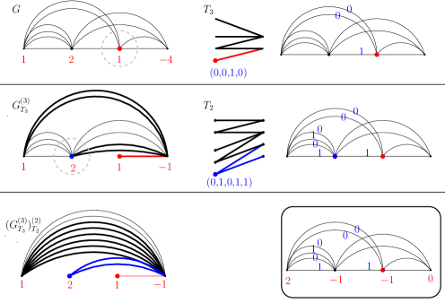
Figure 4. Example of a path in the CCRT $R^{\leftarrow}_{G}$. The graph $G$ is the top left graph. The bottom left graph, $G(8,2,1)$, is a leaf of the CCRT. The compounded reductions performed in order to arrive to this copy of $G(8,2,1)$ are encoded by the trees/compositions $T_{3}$ (at vertex $3$) and $T_{2}$ (at vertex $2$). The correspondence $\Phi$ in the proof of Lemma 4.1 encodes this path as the integral flow on $G$ at the bottom right.

4.2. Encoding the leaves of the CCRT

By Lemma 3.6 only the graphs $G({\bf m})$ appear as leaves of the CCRT ${R^{\leftarrow}_{G}}$. Let $N^{\leftarrow}_{G}({\bf m})$ be the number of times the leaf $G({\bf m})$ appears in ${R^{\leftarrow}_{G}}$. The next key lemma shows that this number is given by a value of the Kostant partition function. This result is a generalization of [15, Thm. 6.1].

Lemma 4.1.

Let $G({\bf m})$ be a full dimensional leaf of the reduction tree ${R^{\leftarrow}_{G}}$ of $\mathcal{F}_{G}({\bf a})$. Then the number of times the leaf $G({\bf m})$ appears in $R_{G}^{\leftarrow}$ is

(4.1) $$N^{\leftarrow}_{G}({\bf m})=K_{G}(m_{1}-{\rm outd}_{1},m_{2}-{\rm outd}_{2},\ldots,m_{n}-{\rm outd}_{n},0),$$

where ${\rm outd}_{i}$ is the outdegree of vertex $i$ in $G$.

The proof of this lemma will use the following result about the edges of the graphs $G_{T}^{(i)}$ appearing in $R_{G}^{\leftarrow}$.

Proposition 4.2.

Given graphs $G$ and $G^{(i)}_{T}$ as above with $a_{i}\geq 0$ and $k<i$ we have that

• the incoming edges $\mathcal{I}_{k}(G^{(i)}_{T})$ and $\mathcal{I}_{k}(G)$ are equal,

• if $T$ is given by the composition $(b_{e},m_{i}-1)_{e\in\mathcal{I}_{i}(G)}$, then $G^{(i)}_{T}$ has $b_{e}+1$ edges $edge(\cdot,e)$ one of which corresponds to the original edge $e$ in $G$ and $b_{e}$ extra edges.

Proof.

This follows from the construction of $G_{T}^{(i)}$. ∎

Example 4.3.

In Figure 4 the graph $G_{T_{3}}^{(3)}$ has the same incoming edges to vertex $1$ as graph $G$. The tree $T_{3}$ is given by the composition $(0,0,1,0)$. Since in this composition $b_{(2,3)}=1$ then $G_{T_{3}}^{(3)}$ has two edges of the form $edge(\cdot,(2,3))$, which are the two copies of $(2,4)$.

Proof of Lemma 4.1.

In ${R^{\leftarrow}_{G}}$ consider a path from $G$ to a leaf. It is obtained by picking particular trees $T_{n},\ldots,T_{2}$ at the vertices $n,n-1,\ldots,2$ during a compounded reduction. We denote the resulting graphs by $G_{n},G_{n-1},\ldots,G_{2}$, respectively. That is, $G_{i}=(G_{i+1})^{(i)}_{T_{i}}$ where $T_{i}$ is the noncrossing tree encoding the subdivision on vertex $i$ and $G_{n+1}:=G$.

The number $N^{\leftarrow}_{G}({\bf m})$ equals the number of tuples of noncrossing trees ${\bf T}:=(T_{2},\ldots,T_{n})$ where the tree $T_{i}$ is such that $G_{i}=(G_{i+1}^{(i)})_{T_{i}}$ and $\deg_{T_{i}}(i)=m_{i}$. We give a correspondence between tuples ${\bf T}$ and integral flows $\mathbf{f}_{G}$ on $G$ with netflow

$${\bf a}({\bf m}):=(m_{1}-{\rm outd}_{1},\ldots,m_{n}-{\rm outd}_{n},0),$$

where $m_{1}=\#E(G)-\sum_{i=2}^{n}m_{i}$.

For $i=n,n-1,\ldots,2$, by Proposition 4.2(i) we have that $\mathcal{I}_{i}(G_{i+1})=\mathcal{I}_{i}(G)$, thus we can encode the tree $T_{i}$ as the composition of $\#\mathcal{O}_{i}(G_{i+1})-1$ of the form $(b_{e},m_{i}-1)_{e\in\mathcal{I}_{i}(G)}$. With this setup set $f(e)=b_{e}$, and set zero flow $f((\cdot,n+1))=0$ on the incoming edges to vertex $n+1$. This defines an integral flow ${\bf f}_{G}$ on $G$. Finally, set $\Phi({\bf T})={\bf f}_{G}$. For an example of $\Phi$, see Figure 4.

Next, we calculate the netflow of the integral flow ${\bf f}_{G}$. For each $i=2,\ldots,n$, by construction of ${\bf f}_{G}$ we have that

(4.2) $$\sum_{e\in\mathcal{I}_{i}(G)}f(e)={\rm outd}_{i}(G_{i+1})-m_{i}.$$

By Proposition 4.2(ii), the outgoing edges of vertex $i$ in $G_{i+1}$ correspond to the original outgoing edges in $\mathcal{O}_{i}(G)$ and extra $b_{(i,j)}$ edges coming from the composition corresponding to the tree $T_{j}$ and edge $(i,j)$ in $\mathcal{I}_{j}(G_{j+1})=\mathcal{I}_{j}(G)$. Since this edge $(i,j)$ of $G_{j+1}$ is also an edge in $\mathcal{O}_{i}(G)$ then we have that

(4.3) $${\rm outd}_{i}(G_{i+1})={\rm outd}_{i}(G)+\sum_{e\in\mathcal{O}_{i}(G)}f(e).$$

Combining (4.2) and (4.3) we obtain that the netflow of vertex $i$ in ${\bf f}_{G}$ is $m_{i}-{\rm outd}_{i}(G)$. Next we calculate the netflow on vertex $1$. Since $G_{2}=G({\bf m})$ then ${\rm outd}_{1}(G_{2})=m_{1}$. Also, by the previous argument (4.3) holds for $i=1$, thus

$$\sum_{e\in\mathcal{O}_{1}(G_{2})}f(e)=m_{1}-{\rm outd}_{1}(G),$$

as desired.

Next we show that $\Phi$ is a bijection by building its inverse. Given a flow ${\bf f}_{G}$ with netflow ${\bf a}({\bf m})$, we read off the flows on the edges $\mathcal{I}_{i}(G)$ for $i=2,\ldots,n$ to obtain compositions of ${\rm outd}_{i}(G)-1+\sum_{e\in\mathcal{O}_{i}(G)}b(e)$ of the form $(b_{e},m_{i}-1)_{e\in\mathcal{I}_{i}(G)}$ if $m_{i}>0$ or of the form $(b_{e})_{e\in\mathcal{I}_{i}(G)}$ if $m_{i}=0$. We encode these compositions as bipartite noncrossing trees $T_{2},\ldots,T_{n}$. By construction and (4.3), the number of outgoing vertices of $T_{i}$ is ${\rm outd}_{i}(G_{i})$. We set $\Psi({\bf f}_{G})=(T_{2},\ldots,T_{n})$. By construction one can show that $\Psi=\Phi^{-1}$, thus $\Phi$ is a bijection. This shows that $N^{\leftarrow}_{G}({\bf m})$ equals the number of integral flows on $G$ with netflow ${\bf a}({\bf m})$. ∎

4.3. Which $G({\bf m})$ appear as leaves in the CCRT

The next result characterizes the vectors ${\bf m}$ encoding the full dimensional leaves of the reduction tree $R_{G}^{\leftarrow}$ of the flow polytope $\mathcal{F}_{G}({\bf a})$.

Theorem 4.4.

Given a flow polytope $\mathcal{F}_{G}({\bf a})$, ${\bf a}=(a_{1},\ldots,a_{n},-\sum_{i=1}^{n}a_{i})$, $a_{i}\in\mathbb{Z}_{\geq 0}$, the graph $G({\bf m})$ is a full dimensional leaf of the CCRT $R^{\leftarrow}_{G}$ if and only if ${\bf m}=(m_{1},\ldots,m_{n})$ is a composition of $\#E(G)$ and $(m_{1},\ldots,m_{n})\geq({\rm outd}_{1},\ldots,{\rm outd}_{n})$ in dominance order.

This result is proved via two lemmas.

Lemma 4.5.

Let $G({\bf m})$ be a full dimensional leaf of the CCRT ${R^{\leftarrow}_{G}}$. Then $(m_{1},\ldots,m_{n})\geq({\rm outd}_{1},\ldots,{\rm outd}_{n})$ in dominance order.

Lemma 4.6.

If ${\bf m}=(m_{1},\ldots,m_{n})$ is a composition of $\#E(G)$ with $(m_{1},\ldots,m_{n})\geq({\rm outd}_{1},\ldots,{\rm outd}_{n})$ in dominance order, then the CCRT $R_{G}^{\leftarrow}$ has full dimensional leaves $G({\bf m})$.

Proof of Theorem 4.4.

The characterization follows by Lemmas 4.5 and 4.6. ∎

The rest of this subsection is devoted to the proofs of the two lemmas.

Proof of Lemma 4.5.

By Lemma 3.6 we know that $m_{1}+\cdots+m_{n}={\rm outd}_{1}+\cdots+{\rm outd}_{n}$. Since these sums are equal, showing $(m_{1},\ldots,m_{n})\geq({\rm outd}_{1},\ldots,{\rm outd}_{n})$ is equivalent to showing $(m_{n},\ldots,m_{1})\leq({\rm outd}_{n},\ldots,{\rm outd}_{1})$. We show the latter by induction on the number of vertices of $G$ with incoming edges.

We first show that $m_{n}\leq{\rm outd}_{n}$. The first reduction in $R_{G}^{\leftarrow}$ occurs at vertex $n$ of $G$ and yields a graph $G^{(n)}_{T}$ with no incoming edges to vertex $n$. If $a_{n}=0$ then $m_{n}=1$ and so the inequality holds (since we require ${\rm outd}_{i}\geq 1$ for all $i\in[n]$). If $a_{n}>0$ then the tree $T$ has left vertices $\mathcal{I}_{n}\cup\{v_{n}\}$ and right vertices $\mathcal{O}_{n}$ with $\deg_{T}(v_{n})=m_{n}$. Thus $m_{n}\leq\#\mathcal{O}_{n}={\rm outd}_{n}$. Also compared to $G$, the graph $G^{(n)}_{T}$ has ${\rm outd}_{n}-m_{n}$ new edges $(i,n+1)$ for $i<n$. Thus

$$({\rm outd}^{\prime}_{1}+\cdots+{\rm outd}^{\prime}_{n-1})-({\rm outd}_{1}+\cdots+{\rm outd}_{n-1})={\rm outd}_{n}-m_{n},$$

where ${\rm outd}^{\prime}_{i}$ is the outdegree of vertex $i$ in $G^{(n)}_{T}$. So for $k=1,\ldots,n-2$ we have

(4.4) $${\rm outd}^{\prime}_{n-1}+{\rm outd}^{\prime}_{n-2}+\cdots+{\rm outd}^{\prime}_{n-k}\leq\left({\rm outd}_{n-1}+\cdots+{\rm outd}_{n-k}\right)+{\rm outd}_{n}-m_{n}.$$

If $G(m_{1},\ldots,m_{n})$ is a full dimensional leaf of ${R^{\leftarrow}_{G}}$ then $G^{(n)}_{T}(m_{1},\ldots,m_{n-1})$ is a full dimensional leaf of the reduction tree ${R^{\leftarrow}_{G^{(n)}_{T}}}$. By induction we have $(m_{n-1},\ldots,m_{2},m_{1})\leq({\rm outd}^{\prime}_{n-1},\ldots,{\rm outd}^{\prime}_{1})$. This combined with (4.4) gives

$$m_{n-1}+m_{n-2}+\cdots+m_{n-k} \leq{\rm outd}^{\prime}_{n-1}+{\rm outd}^{\prime}_{n-2}+\cdots+{\rm outd}^{\prime}_{n-k}$$

$$\leq{\rm outd}_{n}+{\rm outd}_{n-1}+\cdots+{\rm outd}_{n-k}-m_{n}.$$

Thus $(m_{n},\ldots,m_{1})\leq({\rm outd}_{n},\ldots,{\rm outd}_{1})$ as desired. ∎

We now prove the converse of the previous lemma.

Proof of Lemma 4.6.

Since $m_{1}+\cdots+m_{n}={\rm outd}_{1}+\cdots+{\rm outd}_{n}$, then $(m_{1},\ldots,m_{n})\geq({\rm outd}_{1},\ldots,{\rm outd}_{n})$ is equivalent to $(m_{n},\ldots,m_{1})\leq({\rm outd}_{n},\ldots,{\rm outd}_{1})$. We show the result by induction on the number of vertices of $G$ with incoming edges. Let $T$ be the tree encoded by the composition $(0^{{\rm ind}_{n}-1},{\rm outd}_{n}-m_{n},m_{n}-1)$. By Lemma 3.4 the graph $G_{T}^{(n)}$ is a node of the reduction tree $R_{G}^{\leftarrow}$. This graph has $\#E(G)-n-m_{n}$ edges, no incoming edges to vertex $n$ and if ${\rm outd}^{\prime}_{i}$ is the outdegree of vertex $i$ in $G_{T}^{(n)}$ then

(4.5) $${\rm outd}^{\prime}_{n-1}={\rm outd}_{n-1}+{\rm outd}_{n}-m_{n}.$$

Now, the weak composition $(m_{n-1},\ldots,m_{1})$ of $\#E(G)-n-m_{n}$ is $\leq({\rm outd}^{\prime}_{n-1},\ldots,{\rm outd}^{\prime}_{1})$ in dominance order since by (4.5)

$${\rm outd}^{\prime}_{n-1}+\cdots+{\rm outd}^{\prime}_{n-k}={\rm outd}_{n-1}+\cdots+{\rm outd}_{n-k}+{\rm outd}_{n}-m_{n}\geq m_{n-1}+\cdots+m_{n-k}.$$

By induction $G_{T}^{(n)}(m_{1},\ldots,m_{n-1})=G({\bf m})$ is a full dimensional leaf of the reduction tree of $G_{T}^{(n)}$. Since $G_{T}^{(n)}$ is a node of the reduction tree of $G$ then $G({\bf m})$ is a full dimensional leaf of the reduction tree $R_{G}^{\leftarrow}$ as desired. ∎

4.4. Computing the volume of $\mathcal{F}_{G}({\bf a})$

To finish the proof of the Lidskii volume formula (1.1) we fix the reduction tree $R_{G}^{\leftarrow}$ to subdivide $\mathcal{F}_{G}({\bf a})$ into full dimensional leaves $\mathcal{F}_{G({\bf m})}({\bf a})$. Then

$${\rm vol}(\mathcal{F}_{G}({\bf a}))=\sum_{{\bf m}}{\rm vol}(\mathcal{F}_{G({\bf m})}({\bf a}))\cdot N^{\leftarrow}_{G}.$$

The relation (1.1) then follows by using Lemma 3.9 to compute ${\rm vol}(\mathcal{F}_{G({\bf m})}({\bf a}))$, and using Lemma 4.1 to compute $N^{\leftarrow}_{G}$, and relabeling $m_{i}$ to $j_{i}+1$. The compositions ${\bf j}$ add up to ${\rm out}_{1}+\cdots+{\rm out}_{n}=m-n$ and they are exactly those that are $\geq({\rm out}_{1},\ldots,{\rm out}_{n})$ in dominance order by Theorem 4.4.

Example 4.7.

The reduction tree in Figure 3 is in fact $R_{k_{4}}^{\leftarrow}$. Since for $k_{4}$ we have that $({\rm out}_{1},{\rm out}_{2},{\rm out}_{3})=(2,1,0)$, the Lidskii formula (1.1) gives

$${\rm vol}\mathcal{F}_{k_{4}}({\bf 1})=\binom{3}{2,1,0}K_{k_{4}}(2-2,1-1,0-0,0)+\binom{3}{3,0,0}K_{k_{4}}(3-2,0-1,0-0,0)=3\cdot 1+1\cdot 1=4.$$

This corresponds to a subdivision of the polytope $\mathcal{F}_{k_{4}}(1,1,1,-3)$ by the plane $f_{12}=f_{24}$ as indicated by the reduction tree in Figure 3. See Figure 5 for an illustration of this subdivision. For more examples, see Appendix A.

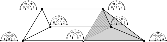
Figure 5. Canonical subdivision of the polytope $\mathcal{F}_{k_{4}}(1,1,1,-3)$ with volume $4$ and $7$ lattice points.

4.5. Alternative volume formula in terms of indegrees

In this section we apply the symmetry of the Kostant partition function (Corollary 2.4) to prove Corollary 1.3 which gives an indegree formula for the volume of flow polytopes.

Proof of Corollary 1.3.

Using Proposition 2.3 and (1.1) we get

$${\rm vol}\mathcal{F}_{G}(\sum_{i=1}^{n}b_{i},-b_{1},\ldots,-b_{n}) ={\rm vol}\mathcal{F}_{G^{r}}(b_{n},\ldots,b_{1},-\sum_{i=1}^{n}b_{i})$$

$$=\sum_{{\bf j}}\binom{m-k-n}{j_{1},\ldots,j_{n}}b_{n}^{j_{n}}\cdots b_{1}^{j_{1}}K_{G^{r}}(j_{n}-{\rm outd}_{1}^{G^{r}}+1,\ldots,j_{1}-{\rm outd}_{n}^{G^{r}}+1,0).$$

Using Corollary 2.4 on the RHS above we get:

$${\rm vol}\mathcal{F}_{G}(\sum_{i=1}^{n}b_{i},-b_{1},\ldots) =\sum_{{\bf j}}\binom{m-k-n}{j_{1},\ldots,j_{n}}b_{1}^{j_{n}}\cdots b_{n}^{j_{1}}K_{G}(0,{\rm outd}_{n}^{G^{r}}-j_{1}-1,\ldots,{\rm outd}_{1}^{G^{r}}-j_{n}-1)$$

$$=\sum_{{\bf j}}\binom{m-k-n}{j_{1},\ldots,j_{n}}b_{1}^{j_{1}}\cdots b_{n}^{j_{n}}K_{G}(0,{\rm ind}_{2}^{G}-j_{1}-1,\ldots,{\rm ind}_{n+1}^{G}-j_{n}-1),$$

where the last equality follows since the outdegree of vertex $i$ in $G^{r}$ equals the indegree of vertex $n+2-i$ in $G$. ∎

5. Proof of the Lidskii formulas for lattice points

In this section we prove the Lidskii formulas (1.2) and (1.3) for the number of lattice points of flow polytopes. The key to our combinatorial proof of (1.2) lies in comparing the basic and compounded reduction trees of the graph $G$, as we do below.

5.1. The basic reduction tree revisited

There are two important properties of a BRT:

• By Proposition 3.1 we get a subdivision of the original flow polytope from the leaves of a BRT.

• Unlike in a CRT, in a BRT we obtain leaves that are not necessarily full dimensional.

The following lemma is implicit in [15, §5.3]:

Lemma 5.1.

Given the CCRT for a graph $G$ on the vertex set $[n+1]$, there is a BRT whose full dimensional leaves coincide with those of the CCRT.

Proof.

(Sketch) Construct the desired BRT by doing basic reductions on vertices $n,\ldots,2$ in this order. At each vertex $i$ repeatedly do BR on the longest possible edges available, until there are still edges on which the BR can be performed. (The length of an edge $(i,j)$ is $j-i$.) When there are no more edges proceed the same way at vertex $i-1$. ∎

Example 5.2.

Figure 6 has an example of a BRT where the full dimensional leaves are boxed. Note that in Figure 3 we subdivided the same flow polytope with the CCRT and got the same leaves as the full dimensional leaves in this BRT.

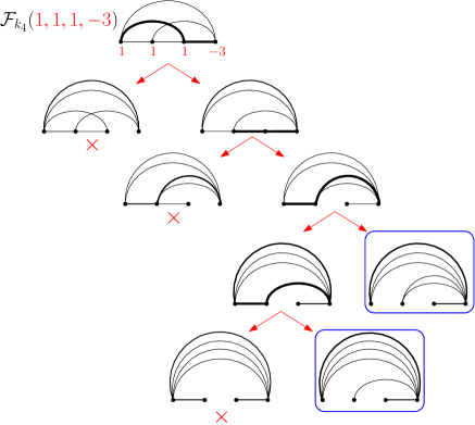
Figure 6. Basic reduction tree (BRT) for the polytope $\mathcal{F}_{k_{4}}(1,1,1-3)$. The full-dimensional leaves are boxed while the lower dimensional are marked by ${\color[rgb]{1,0,0}\times}$. Note that in Figure 3 we subdivided the same flow polytope with the CRT and got the same leaves as the full dimensional leaves in this BRT demonstrating Lemma 5.1.

5.2. Encoding the leaves of the BRT for the Kostant partition function

By (2.4) the function $K_{G}({\bf a})$ is obtained by the following sums of coefficient extractions

(5.1) $$K_{G}({\bf a})=[{\bf x}^{\bf a}]{\prod_{(i,j)\in E(G)}}(1-x_{i}x_{j}^{-1})^{-1},$$

where ${\bf x}^{\bf a}=x_{1}^{a_{1}}\cdots x_{n+1}^{a_{n+1}}$. The advantage of considering the BRT for obtaining (1.2) is that the reduction rule (BR) can easily be encoded with variables as follows.

(5.2) $$\frac{1}{1-x_{a}x_{i}^{-1}}\frac{1}{1-x_{i}x_{b}^{-1}}=\frac{1}{1-x_{a}x_{b}^{-1}}\left(\frac{x_{a}x_{i}^{-1}}{1-x_{a}x_{i}^{-1}}+\frac{1}{1-x_{i}x_{b}^{-1}}\right).$$

We fix a BRT $R_{G}$ whose full dimensional leaves coincide with those of CCRT $R_{G}^{\leftarrow}$. When executing a BR on a graph $G$ as defined in Section 3.1, we draw the BRT by letting $G_{1}$ be the left child and $G_{2}$ be the right child of $G$. We assign the monomial $x_{a}x_{i}^{-1}$ to the “left” edge connecting $G$ and $G_{1}$ and the constant $1$ to the “right”edge connecting $G$ and $G_{2}$. We assign each node $H$ of the BRT the monomial ${\bf x}^{\bf H}$ obtained by multiplying the monomials assigned to the left edges on the unique path from the root of the BRT to $H$. We then have the following expression for $K_{G}({\bf a})$.

(5.3) $$K_{G}({\bf a})=\sum_{H}[{\bf x}^{{\bf a}}]\,\,{\bf x}^{\bf H}\prod_{(i,j)\in E(H)}(1-x_{i}x_{j}^{-1})^{-1}=\sum_{H}K_{H}({\bf a}-{\bf H}),$$

where the sum is over the leaves $H$ of the BRT.

Proposition 5.3.

The monomial ${\bf x}^{\bf H}$ associated to a leaf $H$ of the BRT $R_{G}$ equals

(5.4) $${\bf x}^{\bf H}=\prod_{i=1}^{n}x_{i}^{{\rm outd}_{i}(H)-{\rm outd}_{i}},$$

where ${\rm outd}_{i}(H)$ is the outdegree of vertex $i$ in $H$.

Proof.

At each left step of the BRT involving a reduction on a vertex $i$, an extra edge $(a,b)$ is added that is outgoing with respect to $a$, an outgoing edge $(i,b)$ is removed from the graph, and we record the remaining incoming edge $(a,i)$ in the numerator as $x_{a}x_{i}^{-1}$. This monomial in the numerator records adding an outgoing edge to $a$ and removing an outgoing edge to $i$. Thus the power of $x_{i}$ in the monomial ${\bf x}^{\bf H}$ is the number of extra outgoing edges $(i,\cdot)$ in $H$. This number equals ${\rm outd}_{i}(H)-{\rm outd}_{i}(G)$. ∎

By Lemmas 3.6 and 5.1, the full dimensional leaves of the BRT $R_{G}$ are the graphs $G({\bf m})$. Next we calculate the contribution from each such leaf in (5.3).

Lemma 5.4.

For a full dimensional leaf $G({\bf m})$ of the BRT $R_{G}$ we have that,

$$K_{G({\bf m})}({\bf a}-{\bf G({\bf m})})=\binom{a_{1}+{\rm outd}_{1}-1}{m_{1}-1}\binom{a_{2}+{\rm outd}_{2}-1}{m_{2}-1}\cdots\binom{a_{n}+{\rm outd}_{n}-1}{m_{n}-1}.$$

Proof.

We calculate

$$K_{G({\bf m})}({\bf a}-{\bf G({\bf m})})=[{\bf x}^{\bf a}]\,{\bf x}^{G({\bf m})}\prod_{(i,j)\in E(G({\bf m}))}(1-x_{i}x_{j}^{-1})^{-1}.$$

By Proposition 5.3, the monomial for the full dimensional leaf $G({\bf m})$ is $\prod_{i=1}^{n}x_{i}^{m_{i}-{\rm outd}_{i}}$. Next, we do the coefficient extraction to obtain the desired formula:

$$[{\bf x}^{\bf a}]\prod_{i=1}^{n}\frac{x_{i}^{m_{i}-{\rm outd}_{i}}}{(1-x_{i}x_{n+1}^{-1})^{m_{i}}} =[x_{1}^{a_{1}-m_{1}+{\rm outd}_{1}}\cdots x_{n}^{a_{n}-m_{n}+{\rm outd}_{n}}]\prod_{i=1}^{n}\frac{1}{(1-x_{i})^{m_{i}}}$$

$$=\prod_{i=1}^{n}[x_{i}^{a_{i}-m_{i}+{\rm outd}_{i}}](1-x_{i})^{-m_{i}}=\prod_{i=1}^{n}\binom{a_{i}+{\rm outd}_{i}-1}{m_{i}-1}.$$

∎

Next, we show that the lower dimensional leaves do not contribute to (5.3).

Lemma 5.5.

For a lower dimensional leaf $H$ of the BRT $R_{G}$ we have that $K_{H}({\bf a}-{\bf H})=0$.

Proof.

We calculate $[{\bf x}^{{\bf a}}]\,\,{\bf x}^{H}\prod_{(i,j)\in E(H)}(1-x_{i}x_{j}^{-1})^{-1}$ for a lower dimensional leaf $H$. By Proposition 5.3 the monomial for such leaf $H$ is $\prod_{j=1}^{n}x_{j}^{{\rm outd}_{j}(H)-{\rm outd}_{j}}$. Since the leaf $H$ is not of the form $G({\bf m})$ then it has a vertex $k$ with incoming edges but no outgoing edges. Thus

$$[{\bf x}^{{\bf a}}]\,\,{\bf x}^{H}\prod_{(i,j)\in E(H)}(1-x_{i}x_{j}^{-1})^{-1} =[\prod_{i}x_{i}^{a_{i}-{\rm outd}_{i}(H)+{\rm outd}_{i}}]\prod_{(i,j)\in E(H)}(1-x_{i}x_{j}^{-1})^{-1}$$

$$=K_{H}(a_{1}-{\rm outd}_{1}(H)+{\rm outd}_{1},\ldots,\,a_{k}+{\rm outd}_{k}\,,\ldots).$$

However, since vertex $k$ has no outgoing edges then there are no integral flows in $H$ with netflow $a_{k}+{\rm outd}_{k}>0$ in vertex $k$. (Recall that the graphs $G$ we consider have ${\rm outd}_{i}>0$ for all $i\in[n]$.) ∎

5.3. Counting the lattice points of $\mathcal{F}_{G}({\bf a})$

We now complete the proof of the Lidskii formula (1.2) for $K_{G}({\bf a})$.

Proof of (1.2).

By Lemma 5.5, in (5.3) only the full dimensional leaves contribute

$$K_{G}({\bf a})=\sum_{{\bf m}}K_{G({\bf m})}(a_{1}-m_{1}-{\rm outd}_{1},\ldots,a_{n}-m_{n}-{\rm outd}_{n})\cdot N^{\leftarrow}_{G}$$

We then use Lemma 4.1 to compute $N^{\leftarrow}_{G}$ and Lemma 5.4 to compute $K_{G({\bf m})}(\cdot)$,

$$K_{G}({\bf a}) =\sum_{{\bf m}}K_{G({\bf m})}(a_{1}-m_{1}-{\rm outd}_{1},\ldots,a_{n}-m_{n}-{\rm outd}_{n})\cdot K_{G}(f_{1}({\bf m}),\ldots,f_{n}({\bf m}),0)$$

$$=\sum_{{\bf m}}\binom{a_{1}+{\rm outd}_{1}-1}{m_{1}-1}\cdots\binom{a_{n}+{\rm outd}_{n}-1}{m_{n}-1}\cdot K_{G}(m_{1}-{\rm outd}_{1},\ldots,m_{n}-{\rm outd}_{n},0).$$

∎

Example 5.6.

Continuing with Example 4.7, the graph $k_{3}$ Lidskii formula (1.2) gives

$$K_{k_{4}}(1,1,1,-3)=\binom{3}{2}\binom{2}{1}K_{k_{4}}(0,0,0,0)+\binom{3}{3}\binom{2}{0}K_{k_{4}}(1,-1,0,0)=6+1=7.$$

The subdivision of $\mathcal{F}_{k_{4}}(1,1,1,-3)$ in Figure 5 yields two cells with six and four lattice points each and three lattice points in their intersection. These three points are only counted in the first cell. For more examples, see Appendix A.

By applying the symmetry of the Kostant partition function we obtain an alternative formula to (1.2).

Corollary 5.7.

Let $G$ be a graph on the vertex set $[n+1]$ with at least one incoming edge at vertex $i$ for $i=2,\ldots,n+1$, and let ${\bf b}=(\sum_{i=1}^{n}b_{i},-b_{1},\ldots,-b_{n})$ with $b_{i}\in\mathbb{Z}_{\geq 0}$, then

(5.5) $$K_{G}({\bf{\bf b}})=\sum_{{{\bf j}}}\binom{b_{1}+{\rm in}_{2}}{j_{1}}\cdots\binom{b_{n}+{\rm in}_{n+1}}{j_{n}}\cdot K_{G}(0,{\rm in}_{2}-j_{1}-1,{\rm in}_{3}-i_{2}-1,\ldots,{\rm in}_{n+1}-j_{n}-1),$$

where the sum is over weak compositions ${\bf j}=(j_{1},j_{2},\ldots,i_{n})$ of $m-n$ that are $\leq$ $({\rm in}_{2},\ldots,{\rm in}_{n+1})$ in dominance order..

Proof.

The result follows by applying Corollary 2.4 to (1.2) (cf. proof of Corollary 1.3). ∎

5.4. Proof of the Lidskii formula (1.3) for lattice points

Next we prove the alternative Lidskii formula (1.3) for the Kostant partition function. We first prove the results for the case $a_{i}\geq{\rm ind}_{i}(G)$ for $i=1,\ldots,n$ and then extend them to the range $0\leq a_{i}<{\rm ind}_{i}(G)$ using the polynomiality property of the Kostant partition function.

The result follows mostly the same argument that proves (1.2) but instead of (5.2), we encode the reduction rule (BR) as

(5.6) $$\frac{1}{1-x_{a}x_{i}^{-1}}\frac{1}{1-x_{i}x_{b}^{-1}}=\frac{1}{1-x_{a}x_{b}^{-1}}\left(\frac{1}{1-x_{a}x_{i}^{-1}}+\frac{x_{i}x_{b}^{-1}}{1-x_{i}x_{b}^{-1}}\right).$$

We fix a BRT $R_{G}$ whose full dimensional leaves coincide with those of CCRT $R_{G}^{\leftarrow}$. When executing a BR on a graph $G$ as defined in Section 3.1, we draw the BRT by having $G_{1}$ be the left child and $G_{2}$ be the right child of $G$. We assign the constant $1$ to the “right”edge connecting $G$ and $G_{1}$, and the monomial $x_{i}x_{b}^{-1}$ to the “right” edge connecting $G$ and $G_{2}$. Then the analogue of (5.3) is

(5.7) $$K_{G}({\bf a})=\sum_{H}[{\bf x}^{\bf a}]\,{\bf x}^{\bf H^{\prime}}\prod_{(i,j)\in E(H)}(1-x_{i}x_{j}^{-1}){-1}=\sum_{H}K_{H}({\bf a}-{\bf H}^{\prime}),$$

where the sum is over all leaves of the BRT $R_{G}$.

Proposition 5.8.

The monomial ${\bf x}^{\bf H^{\prime}}$ associated to a leaf $H$ of the BRT $R_{G}$ equals

$${\bf x}^{\bf H^{\prime}}=\prod_{j=2}^{n+1}x_{j}^{{\rm ind}_{j}-{\rm ind}_{j}(H)}.$$

Proof sketch.

This monomial comes from the right steps in the reduction tree, where an incoming edge $(a,i)$ is removed and we record the outgoing edge $(i,b)$ in the numerator as $x_{i}x_{b}^{-1}$. ∎

As in the proof of (1.2), the full dimensional leaves of the BRT $R_{G}$ are the graphs $G({\bf m})$. Next we calculate the contribution from each such leaf in (5.7).

Lemma 5.9.

Let ${\bf a}=(a_{1},\ldots,a_{n},-\sum_{i=1}^{n}a_{i})$ with $a_{i}\in\mathbb{Z}_{\geq 0}$ with $a_{i}\geq{\rm ind}_{i}(G)$. For a full dimensional leaf $G({\bf m})$ of the BRT $R_{G}$ we have that

$$K_{G({\bf m})}({\bf a}-{\bf G({\bf m})^{\prime}})=\mathchoice{\left(\kern-5.0pt{\binom{a_{1}-{\rm ind}_{1}+1}{m_{1}-1}}\kern-5.0pt\right)}{\bigl{(}\kern-3.00003pt{\binom{a_{1}-{\rm ind}_{1}+1}{m_{1}-1}}\kern-3.00003pt\bigr{)}}{\bigl{(}\kern-3.00003pt{\binom{a_{1}-{\rm ind}_{1}+1}{m_{1}-1}}\kern-3.00003pt\bigr{)}}{\bigl{(}\kern-3.00003pt{\binom{a_{1}-{\rm ind}_{1}+1}{m_{1}-1}}\kern-3.00003pt\bigr{)}}\cdots\mathchoice{\left(\kern-5.0pt{\binom{a_{n}-{\rm ind}_{n}+1}{m_{n}-1}}\kern-5.0pt\right)}{\bigl{(}\kern-3.00003pt{\binom{a_{n}-{\rm ind}_{n}+1}{m_{n}-1}}\kern-3.00003pt\bigr{)}}{\bigl{(}\kern-3.00003pt{\binom{a_{n}-{\rm ind}_{n}+1}{m_{n}-1}}\kern-3.00003pt\bigr{)}}{\bigl{(}\kern-3.00003pt{\binom{a_{n}-{\rm ind}_{n}+1}{m_{n}-1}}\kern-3.00003pt\bigr{)}}.$$

Proof.

By Proposition 5.8 the monomials for each full dimensional leaf $G({\bf m})$ are the same:

$$x_{n+1}^{m}\prod_{j=1}^{n+1}x_{j}^{{\rm ind}_{j}(G)}.$$

(For convenience, we included superflously the variable $x_{1}$ since ${\rm ind}_{1}(G)=0$.) Thus

$$[{\bf x}^{\bf a}]\prod_{j=1}^{n}\frac{x_{j}^{{\rm ind}_{j}}}{(1-x_{j}x_{n+1}^{-1})^{m_{j}}}=\prod_{j=1}^{n}\left([x_{j}^{a_{j}-{\rm ind}_{j}}](1-x_{j})^{-m_{j}}\right)=\prod_{j=1}^{n}\binom{a_{j}-{\rm ind}_{j}+m_{j}-1}{m_{j}-1},$$

where we used the assumption that $a_{j}-{\rm ind}_{j}\geq 0$ for $j=1,\ldots,n$. ∎

Next, we show that the lower dimensional leaves do not contribute to (5.7).

Lemma 5.10.

Let ${\bf a}=(a_{1},\ldots,a_{n},-\sum_{i=1}^{n}a_{i})$ with $a_{i}\in\mathbb{Z}_{\geq 0}$ with $a_{i}\geq{\rm ind}_{i}(G)$. For a lower dimensional leaf $H$ of the BRT $R_{G}$ we have that $K_{H}({\bf a}-{\bf H}^{\prime})=0$.

Proof.

By Proposition 5.8 the monomial for such leaf $H$ is $\prod_{j=2}^{n+1}x_{j}^{{\rm ind}_{j}-{\rm ind}_{j}(H)}$. Since the leaf $H$ is not of the form $G({\bf m})$ then it has a vertex $k\geq 2$ with incoming but no outgoing edges. Thus

$$[{\bf x}^{\bf a}]\,\,\,{\bf x}^{\bf H^{\prime}}\prod_{(i,j)\in E(H)}(1-x_{i}x_{j}^{-1})^{-1}=K_{H}(a_{1},a_{2}-{\rm ind}_{2}+{\rm ind}_{2}(H),\ldots,a_{k}-{\rm ind}_{k}+{\rm ind}_{k}(H),\ldots).$$

However, since vertex $k$ has no outgoing edges then there are no integral flows in $H$ with netflow $a_{k}-{\rm ind}_{k}+{\rm ind}_{k}(H)>0$ at this vertex. ∎

Proof of (1.3).

We start by assuming that $a_{i}\geq{\rm ind}_{i}(G)$. By Lemma 5.10, in (5.7) only the full dimensional leaves contribute

$$K_{G}({\bf a})=\sum_{\bf m}K_{G({\bf m})}(a_{1}-{\rm ind}_{1},\ldots,a_{n}-{\rm ind}_{n})\cdot N_{G}^{\leftarrow}.$$

We then use Lemma 4.1 to compute $N^{\leftarrow}_{G}$ and Lemma 5.9 to compute $K_{G({\bf m})}(\cdot)$,

$$K_{G}({\bf a}) =\sum_{{\bf m}}K_{G({\bf m})}(a_{1}-{\rm ind}_{1},\ldots,a_{n}-{\rm ind}_{n})\cdot K_{G}(m_{1}-{\rm outd}_{1},\ldots,m_{n}-{\rm outd}_{n},0),$$

$$=\sum_{{\bf m}}\mathchoice{\left(\kern-5.0pt{\binom{a_{1}-{\rm ind}_{1}+1}{m_{1}-1}}\kern-5.0pt\right)}{\bigl{(}\kern-3.00003pt{\binom{a_{1}-{\rm ind}_{1}+1}{m_{1}-1}}\kern-3.00003pt\bigr{)}}{\bigl{(}\kern-3.00003pt{\binom{a_{1}-{\rm ind}_{1}+1}{m_{1}-1}}\kern-3.00003pt\bigr{)}}{\bigl{(}\kern-3.00003pt{\binom{a_{1}-{\rm ind}_{1}+1}{m_{1}-1}}\kern-3.00003pt\bigr{)}}\cdots\mathchoice{\left(\kern-5.0pt{\binom{a_{n}-{\rm ind}_{n}+1}{m_{n}-1}}\kern-5.0pt\right)}{\bigl{(}\kern-3.00003pt{\binom{a_{n}-{\rm ind}_{n}+1}{m_{n}-1}}\kern-3.00003pt\bigr{)}}{\bigl{(}\kern-3.00003pt{\binom{a_{n}-{\rm ind}_{n}+1}{m_{n}-1}}\kern-3.00003pt\bigr{)}}{\bigl{(}\kern-3.00003pt{\binom{a_{n}-{\rm ind}_{n}+1}{m_{n}-1}}\kern-3.00003pt\bigr{)}}\cdot K_{G}(m_{1}-{\rm outd}_{1},\ldots,m_{n}-{\rm outd}_{n},0).$$

Finally, to extend the identity to the cases where $0\leq a_{i}<{\rm ind}_{i}(G)$ we use the polynomiality property of $K_{G}({\bf a})$ (Proposition 2.2). ∎

Example 5.11.

To contrast Example 5.6, for the graph $k_{3}$ we have $({\rm in}_{1},{\rm in}_{2},{\rm in}_{3})=(-1,0,1)$, so the alternative Lidskii formula (1.3), gives

$$K_{k_{4}}(1,1,1,-3)=\binom{3}{2}\binom{1}{1}K_{k_{4}}(0,0,0,0)+\binom{4}{3}\binom{0}{0}K_{k_{4}}(1,-1,0,0)=3+4=7.$$

The subdivision of $\mathcal{F}_{k_{4}}(1,1,1,-3)$ in Figure 5 yields two cells with six and four lattice points each and three lattice points in their intersection. In contrast with Example 5.6, these three points are now counted in the second cell. For more examples, see Appendix A.

6. Enumerative properties of the canonical subdivision and Lidskii formulas

In this section we give enumerative properties of the Lidskii formulas and of the canonical subdivision of flow polytopes $\mathcal{F}_{G}({\bf a})$ we used to prove Theorem 1.1. We illustrate the results with the Stanley–Pitman polytope ($G=\Pi_{n}$), the Baldoni–Vergne polytope ($G=k_{n+1}$), and a generalization of the former (see Section 6.4).

6.1. Number of types of cells in the subdivision

Recall that we call cells the full dimensional polytopes in the canonical subdivision of $\mathcal{F}_{G}({\bf a})$. In this section we assume $a_{i}\in\mathbb{Z}_{>0}$ so that the cells are present. Moreover, two cells are said to be of the same type if they are integrally equivalent.

Theorem 6.1.

The types of cells of the canonical subdivision of $\mathcal{F}_{G}(a_{1},a_{2},\ldots,a_{n},-\sum_{i}a_{i})$ are in one-to-one correspondence with lattice points of $\operatorname{PS}({\rm out}_{n},{\rm out}_{n-1},\ldots,{\rm out}_{2})$.

Proof.

The cells of the canonical subdivision of $\mathcal{F}_{G}({\bf a})$ are characterized by tuples $(j_{1},\ldots,j_{n})$ of nonnegative integers satisfying

$$j_{1}+\dots+j_{k} \geq{\rm out}_{1}+\cdots+{\rm out}_{k},\text{ for }k=1,\ldots,n-1$$

$$j_{1}+\cdots+j_{n} ={\rm out}_{1}+\cdots+{\rm out}_{n}.$$

These conditions are equivalent to

$$j_{n}+j_{n-1}+\dots+j_{n-k+1} \leq{\rm out}_{n}+{\rm out}_{n-1}+\cdots+{\rm out}_{n-k+1},\text{ for }k=1,\ldots,n-1$$

$$j_{1}+\cdots+j_{n} ={\rm out}_{1}+\cdots+{\rm out}_{n},$$

which in turn is equivalent to the tuple $(j_{n},j_{n-1},\ldots,j_{2})$ being a lattice point of the Pitman–Stanley polytope $\operatorname{PS}({\rm out}_{n},{\rm out}_{n-1},\ldots,{\rm out}_{2})$ and $j_{1}=({\rm out}_{1}+\cdots+{\rm out}_{n})-(j_{2}+\cdots+j_{n})$. ∎

Corollary 6.2.

The number $N$ of types of cells of the canonical subdivision of the polytope $\mathcal{F}_{G}({\bf a})$ is the number of plane partitions of shape $({\rm out}_{n},{\rm out}_{n}+{\rm out}_{n-1},\ldots,{\rm out}_{n}+\cdots+{\rm out}_{2})$ with largest part at most $2$ which is given by the following determinant

$$N=\det\left[\binom{{\rm out}_{i+1}+\cdots+{\rm out}_{n}+1}{i-j+1}\right]_{1\leq i,j\leq n-1}.$$

Proof.

The result follows by combining Theorem 6.1 with Theorem 2.8. ∎

We next apply this result to the Pitman–Stanley polytope and the Baldoni–Vergne polytope.

Corollary 6.3.

The number of types of cells of the canonical subdivision of the Pitman–Stanley polytope $\mathcal{F}_{\Pi_{n}}({\bf a})$ is $C_{n}$.

Proof.

For the graph $\Pi_{n}$ we have that ${\rm out}_{i}=1$ so by Corollary 6.2, the number of types of cells of the canonical subdivision equals the number of plane partitions of shape $(1,2,\ldots,n-1)$ with largest part at most 2. These plane partitions are easily seen to be in bijection with Dyck paths of size $n$ (consider the interface between $1$s and $2$s in such a plane partition). ∎

Corollary 6.4.

The number $t_{n}$ of types of cells of the canonical subdivision of the Baldoni–Vergne polytope $\mathcal{F}_{k_{n+1}}({\bf a})$ equals the number of plane partitions of shape $(\binom{2}{2},\binom{3}{2},\ldots,\binom{n-1}{2})$ with largest part at most $2$.The number $t_{n}$ is given by the determinant

(6.1) $$t_{n}=\det\left[\binom{\binom{n-i}{2}+1}{i-j+1}\right]_{1\leq i,j\leq n-1}.$$

Proof.

This is a direct application of Corollary 6.2. For the complete graph $k_{n+1}$ we have that ${\rm out}_{i}=n-i$. ∎

Example 6.5.

The subdivision of $\mathcal{F}_{k_{4}}(1,1,1,-3)$ illustrated in Figure 5 has $t_{3}=2$ types of cells. The subdivision of $\mathcal{F}_{k_{5}}(1,1,1,1,-4)$ has $t_{4}=7$ types of cells as can be calculated via the determinant in (6.1). For the terms of the sequence $(t_{n})_{n\geq 0}$ see [23, A107877].

6.2. Number of cells in the canonical subdivision

Given a graph $G$ on the vertex set $[n+1]$, let $G^{\star}$ and $G^{\circ}$ be the graphs obtained from $G$ by adding a vertex $0$ adjacent to vertices $1,2,\ldots,n$ and adjacent to vertices $1,2,\ldots,n+1$ respectively.

Theorem 6.6.

The following numbers are all equal:

• the number of cells of the canonical subdivision of $\mathcal{F}_{G}(a_{1},a_{2},\ldots,a_{n},-\sum a_{i})$,

• the sum

  (6.2) $$\sum_{{\bf j}}K_{G}(j_{1}-{\rm out}_{1},\ldots,j_{n}-{\rm out}_{n},0),$$

  over compositions ${\bf j}=(j_{1},\ldots,j_{n})$ of $m-n$ that are $\geq({\rm out}_{1},\ldots,{\rm out}_{n})$ in dominance order,

• the number of lattice points of the polytope $\mathcal{F}_{G^{\star}}(n-m,-{\rm out}_{1},\ldots,-{\rm out}_{n},0)$,

• the volume of the polytope $\mathcal{F}_{G^{\star}}(1,0,\ldots,0,-1)$,

• the volume of the polytope $\mathcal{F}_{G^{\circ}}(1,0,\ldots,0,-1)$.

Proof.

From the subdivision in the proof of Theorem 1.1 for $\mathcal{F}_{G}({\bf a})$ the number $P$ of full-dimensional cells of the subdivision is the sum given in (6.2). This proves the equivalence of (a) and (b).

Next we show the equality between (b) and (c). Each term in the sum in (6.2) counts the number of integral flows on $G$ with netflow $(j_{1}-{\rm out}_{1},\ldots,j_{n}-{\rm out}_{n},0)$. Each such flow corresponds to an integral flow on $G^{\circ}$ with netflow $(n-m,-{\rm out}_{1},\ldots,-{\rm out}_{n})$ by assigning a flow of $j_{i}$ to edge $(0,i)$ for $i=1,2,\ldots,n$. Conversely, given an integral flow in $G^{\circ}$ with netflow $(n-m,-{\rm out}_{1},\ldots,-{\rm out}_{n},0)$, if $j_{i}$ is the netflow on edge $(0,i)$ then the integral flows on the edges of the subgraph $G$ yields an integral flow on $G$ with netflow $(j_{1}-{\rm out}_{1},\ldots,j_{n}-{\rm out}_{n},0)$. Thus

$$P=K_{G^{\star}}(n-m,-{\rm out}_{1},\ldots,-{\rm out}_{n},0).$$

This proves the equivalence of (b) and (c).

Next, the numbers in (c) and (d) are equal since (1.5) applied to $\mathcal{F}_{G^{\circ}}(1,0,\ldots,0,-1)$ yields

$${\rm vol}\mathcal{F}_{G^{\star}}(1,0,\ldots,0,-1)=K_{G^{\star}}(n-m,-{\rm out}_{1},\ldots,-{\rm out}_{n},0).$$

Finally, we show the equality between the numbers in (d) and (e) by combining (1.5) with the observation that

$$K_{G^{\star}}(n-m,-{\rm out}_{1},\ldots,-{\rm out}_{n},0)=K_{G^{\circ}}(n-m,-{\rm out}_{1},\ldots,-{\rm out}_{n},0),$$

where ${\rm out}_{i}={\rm out}_{i}(G^{\star})={\rm out}_{i}(G^{\circ})$ for $i=1,\ldots,n$. ∎

Remark 6.7.

In Section 7 we give a second proof of the equality between (a) and (d) in Theorem 6.6 using the Cayley trick [12, 25].

Corollary 6.8 ([21, Thm. 1]).

The number of cells of the canonical subdivision of the Pitman–Stanley polytope $\mathcal{F}_{\Pi_{n}}({\bf a})$ is $C_{n}$.

Proof.

By in Theorem 6.6 (a)$=$(b) the number of cells of the canonical subdivision of $\mathcal{F}_{\Pi_{n}}({\bf a})$ equals the sum

$$P=\sum_{\bf j}K_{\Pi_{n}}(j_{1}-1,\ldots,j_{n}-1,0).$$

By Corollary 6.3 the sum on the RHS above has $C_{n}$ compositions j with nonzero contribution. Each Kostant partition function in the sum has zero netflow on vertex $n+1$. Thus each such term counts integral flows on the path $1\to 2\to\cdots\to n$. There is exactly one such integral flow, so $K_{\Pi_{n}}(j_{1}-1,\ldots,j_{n}-1,0)=1$ for each of the $C_{n}$ many compositions ${\bf j}\geq(1,\ldots,1)$. ∎

Corollary 6.9.

The number of cells of the canonical subdivision of $\mathcal{F}_{k_{n+1}}({\bf a})$ for ${\bf a}\in\mathbb{Z}^{n}_{>0}$ is $C_{0}C_{1}C_{2}\cdots C_{n-1}$.

Proof.

For $G=k_{n+1}$ we have that $G^{\circ}=k_{n+2}$. Then by Theorem 6.6 (a)$=$(d), the desired number of cells equals the volume of the CRY polytope of size $n+1$. The result then follows by (1.7). ∎

Example 6.10.

Continuing with Example 6.5, the subdivision of $\mathcal{F}_{k_{4}}(1,1,1,-3)$ illustrated in Figure 5 has $C_{1}C_{2}=2$ cells ($t_{3}=2$ types of cells, each appearing once). The subdivision of $\mathcal{F}_{k_{5}}(1,1,1,1,-4)$ has $C_{1}C_{2}C_{3}=10$ cells of $t_{4}=7$ different types.

6.3. Number of words in the Lidskii volume formula

If we take the Lidskii formula for the volume of $\mathcal{F}_{G}({\bf a})$ and we look at it as a sum of words $w=w_{1}w_{2}\cdots w_{n}$ in the alphabet $a_{1},a_{2},\ldots$ (the order of letters matters), then (1.1) becomes

(6.3) $${\rm vol}(F_{G}({\bf a}))=\sum_{w}m(w)\cdot w_{1}w_{2}\cdots w_{n}.$$

where $m(w)$ is the multiplicity of the word $w$. See Example 6.14 below. From the Lidskii formula (1.1) the multiplicity is given by a Kostant partition function

$$m(w)=K_{G}(j_{1}-{\rm outd}_{1},\ldots,j_{n}-{\rm outd}_{n},0),$$

where $j_{k}$ is the number of instances of the letter $a_{k}$ in $w$. The following proposition gives the number of such words with multiplicity as a volume of another flow polytope.

Proposition 6.11.

For the flow polytope $\mathcal{F}_{G}({\bf a})$ and the words $w$ as defined above we have that

$$\sum_{w}m(w)={\rm vol}\mathcal{F}_{G}(1,\ldots,1,-n).$$

Proof.

To count the words with multiplicity it suffices to evaluate $a_{i}=1$ in (1.1). ∎

For the Pitman–Stanley polytope the multiplicity of each words $w$ in (6.3) is $m(w)=K_{\Pi_{n}}(j_{1}-1,\ldots,j_{n}-1,0)$. This value of the Kostant partition function equals $1$ as explained in the proof of Corollary 6.8. Moreover, the words appearing in the formula are parking functions as shown in [21].

Corollary 6.12 ([21, Thm. 11]).

For the Pitman–Stanley polytope $\mathcal{F}_{\Pi_{n}}({\bf a})$ we have that

$${\rm vol}\mathcal{F}_{\Pi_{n}}({\bf a})=\sum_{(k_{1},\ldots,k_{n})}a_{k_{1}}a_{k_{2}}\cdots a_{k_{n}},$$

where the sum is over parking functions $(k_{1},\ldots,k_{n})$. Thus the number of words in the Lidskii volume formula is $(n+1)^{n-1}$.

Corollary 6.13.

For the flow polytope $\mathcal{F}_{k_{n+1}}({\bf a})$, the number of words with multiplicity in the Lidskii volume formula equals

$$\sum_{w}m(w)=f^{(n-1,n-2,\ldots,1)}\cdot C_{1}C_{2}\cdots C_{n-1}.$$

Proof.

This number of words is exactly the volume of the Tesler polytope ${\rm vol}\mathcal{F}_{k_{r+1}}({\bf 1})$ given in (1.8). ∎

Example 6.14.

For the graph $G=k_{4}$, omitting from the notation the netflow on the last vertex, we have that

$${\rm vol}\mathcal{F}_{k_{4}}(a_{1},a_{2},a_{3})=\binom{3}{3,0,0}a_{1}^{3}\cdot K_{k_{4}}(1,-1,0)+\binom{3}{2,1,0}a_{1}^{2}a_{2}\cdot K_{k_{4}}(0,0,0),$$

and the polytope subdivides into $K_{k_{4}}(1,-1,0)+K_{k_{4}}(0,0,0)=2$ cells. In terms of words:

$${\rm vol}\mathcal{F}_{k_{4}}(a_{1},a_{2},a_{3})=a_{1}a_{1}a_{1}\cdot K_{k_{4}}(1,-1,0)+(a_{1}a_{1}a_{2}+a_{1}a_{2}a_{1}+a_{2}a_{1}a_{1})\cdot K_{k_{4}}(0,0,0),$$

i.e. the volume formula is given in terms of four words.

Remark 6.15.

It is natural to ask for a characterization of the words that appear in (6.3). In the Pitman-Stanley polytope the equivalent words are parking functions (see Corollary 6.12). See [5] for a recent characterization.

6.4. Flow polytope with volume counted by lattice points of Pitman–Stanley polytope

Given ${\bf c}:=(c_{1},c_{2},\ldots,c_{n})$ for nonnegative integers $c_{i}$, let $\Pi_{n}({\bf c})$ be the graph with vertices $[n+1]$ consisting of the path $1\to 2\to\cdots\to n+1$ and $c_{i}$ multiple edges of the form $(i,n+1)$. Recall that $\Pi_{n}({\bf c})^{\star}$ denotes the graph $\Pi_{n}({\bf c})$ with an additional vertex $0$ adjacent to vertices $1,2,\ldots,n$. See Figure 7. At $c_{1}=\ldots=c_{n}=1$, the graph $\Pi_{n}(1,\ldots,1)$ equals the graph $\Pi_{n}$.

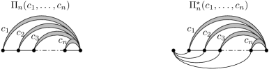
Figure 7. Example of graphs $\Pi_{n}({\bf c})$ and $\Pi_{n}({\bf c})^{\star}$. The gray edges with label $c_{i}$ indicate $c_{i}$ multiple edges.

Corollary 6.16.

Let ${\bf a}=(a_{1},\ldots,a_{n},-\sum_{i}a_{i})$ and ${\bf c}=(c_{1},\ldots,c_{n})$ be tuples of nonnegative integers $a_{i}$ and $c_{i}$. Then the volume and lattice points of the flow polytope $\mathcal{F}_{\Pi_{n}({\bf c})}({\bf a})$ equal

(6.4) $${\rm vol}\mathcal{F}_{\Pi_{n}({\bf c})}({\bf a}) =\sum_{\bf j}\binom{c_{1}+\cdots+c_{n}}{j_{1},\ldots,j_{n}}a_{1}^{j_{1}}\cdots a_{n}^{j_{n}},$$

(6.5) $$K_{\Pi_{n}({\bf c})}({\bf a}) =\sum_{\bf j}\binom{a_{1}+c_{1}}{j_{1}}\cdots\binom{a_{n}+c_{n}}{j_{n}},$$

(6.6) $$=\sum_{\bf j}\mathchoice{\left(\kern-5.0pt{\binom{a_{1}+1}{j_{1}}}\kern-5.0pt\right)}{\bigl{(}\kern-3.00003pt{\binom{a_{1}+1}{j_{1}}}\kern-3.00003pt\bigr{)}}{\bigl{(}\kern-3.00003pt{\binom{a_{1}+1}{j_{1}}}\kern-3.00003pt\bigr{)}}{\bigl{(}\kern-3.00003pt{\binom{a_{1}+1}{j_{1}}}\kern-3.00003pt\bigr{)}}\mathchoice{\left(\kern-5.0pt{\binom{a_{2}}{j_{2}}}\kern-5.0pt\right)}{\bigl{(}\kern-3.00003pt{\binom{a_{2}}{j_{2}}}\kern-3.00003pt\bigr{)}}{\bigl{(}\kern-3.00003pt{\binom{a_{2}}{j_{2}}}\kern-3.00003pt\bigr{)}}{\bigl{(}\kern-3.00003pt{\binom{a_{2}}{j_{2}}}\kern-3.00003pt\bigr{)}}\cdots\mathchoice{\left(\kern-5.0pt{\binom{a_{n}}{j_{n}}}\kern-5.0pt\right)}{\bigl{(}\kern-3.00003pt{\binom{a_{n}}{j_{n}}}\kern-3.00003pt\bigr{)}}{\bigl{(}\kern-3.00003pt{\binom{a_{n}}{j_{n}}}\kern-3.00003pt\bigr{)}}{\bigl{(}\kern-3.00003pt{\binom{a_{n}}{j_{n}}}\kern-3.00003pt\bigr{)}},$$

where the three sums are over weak compositions ${\bf j}=(j_{1},\ldots,j_{n})$ of $\sum_{i}c_{i}$ that are $\geq(c_{1},\ldots,c_{n})$ in dominance order.

Proof.

The result follows by Theorem 1.1 for $G=\Pi_{n}({\bf c})$ with ${\rm outd}_{i}=1$ for $i=1,\ldots,n$, ${\rm in}_{1}=-1,{\rm in}_{j}=0$ for $j=2,\ldots,n$, and noticing that

(6.7) $$K_{\Pi_{n}({\bf c})}(j_{1}-1,\ldots,j_{n}-1,0)=K_{\Pi_{n}}(j_{1}-1,\ldots,j_{n}-1,0)=1,$$

where the second equality follows from the proof of Corollary 6.8. ∎

Corollary 6.17.

Let ${\bf c}=(c_{1},\ldots,c_{n})$ be a tuple of nonnegative integers. and let $\Pi_{n}({\bf c})^{\star}$ be the graph defined above, then

$${\rm vol}\mathcal{F}_{\Pi_{n}({\bf c})^{\star}}(1,0,\ldots,0,-1)=\#(\operatorname{PS}(c_{n},c_{n-1}\ldots,c_{2})\,\cap\,\mathbb{Z}^{n-1})=\det\left[\binom{c_{i+1}+\cdots+c_{n}+1}{i-j+1}\right]_{1\leq i,j\leq n-1}.$$

In particular, the volume is independent of $c_{1}$.

Proof.

The result follows by combining Theorems 6.6 (b)$=$(d), (6.7),  6.1 and Corollary 6.2. ∎

Remark 6.18.

The following particular case of the previous volume formula gives a product. When ${\bf c}=(d,\ldots,d,n)$ is a tuple of size $n+1$, by Corollary 6.17 the volume of $\mathcal{F}_{\Pi_{n+1}(d,\ldots,d,c)^{\star}}(1,0,\ldots,0,-1)$ equals the number of lattice points of $\operatorname{PS}(c,d^{n})$. In [21, Thm. 13], this number of lattice points has a product formula, giving

$${\rm vol}\mathcal{F}_{\Pi_{n+1}(d,\ldots,d,c)^{\star}}(1,0,\ldots,0,-1)=\frac{1}{n!}(c+1)(c+nd+2)(c+nd+3)\cdots(c+nd+n).$$

Remark 6.19.

The volume of the polytope $\mathcal{F}_{\Pi_{n+1}({\bf c})}({\bf 1})$ equals the number of generalized parking functions studied by Yan [26, 27]. Also, the polytope $\mathcal{F}_{\Pi_{n+1}({\bf 1})^{\star}}(1,1,\ldots,1,-n-1)$ appears in [5] and is called the Caracol polytope. Its volume equals $C_{n-1}\cdot(n+1)^{n-1}$.

We finish our treatment of the flow polytope $\mathcal{F}_{\Pi_{n+1}({\bf c})}({\bf a})$ by proving that its Ehrhart polynomial has positive coefficients. This was known for the Pitman–Stanley polytope [21, Eq. (33)]. For more on positivity of coefficients of Ehrhrat polynomials see e.g. [6, 14].

Corollary 6.20.

The Ehrhart polynomial of $\mathcal{F}_{\Pi_{n+1}({\bf c})}({\bf a})$ has positive coefficients.

Proof.

The result follows by the formula (6.6) for the Ehrhart polynomial $K_{\Pi_{n+1}({\bf c})}(t\cdot{\bf a})$. ∎

Remark 6.21.

The positivity in $t$ of the polynomial $K_{G}(t\cdot{\bf a})$ is not apparent from either (1.2) or (1.3). There are examples of graphs $G$ where $K_{G}(t,0,\ldots,0,-t)$ has negative coefficients in $t$ [14, Sec. 4.4]. However, positivity in equation (1.3) holds if $a_{j}\geq{\rm in}_{j}$ for $j=1,\ldots,n$ or if the Kostant partition function on the LHS of these equations is replaced by $1$ and graph $G$ verifies (by Corollary 6.20 with $c_{i}={\rm out}_{i}\geq 0$).

7. The Cayley trick for flow polytopes

Corollary 1.4 and the Lidskii volume formula (1.1) express the volume of flow polytopes in terms of the number of lattice points of several related flow polytopes. The volumes of root polytopes and integer points of generalized permutahedra obey a similar relation, as shown in [22, §14] by Postnikov. Postnikov used the Cayley trick [12, 25] to give the volume of root polytopes in terms of the number of lattice points of generalized permutahedra. The first author and St. Dizier proved a relation between volumes of flow polytopes and integer points of generalized permutahedra [19]. In this section we use the Cayley trick to give a second proof of Theorem 6.6. It would be interesting to use this technique to fully rederive the Lidskii formulas.

We follow the notation in [22, §14]. Given a polytope $P$, its polytopal subdivisions form a poset by refinement whose minimal elements correspond to triangulations. Given a $d$-dimensional Minkowski sum $Q:=P_{1}+\cdots+P_{n}$, a Minkowski cell of $Q$ is a polytope $B_{1}+\cdots+B_{n}$ where $B_{i}$ is a convex hull of a subset of vertices of $P_{i}$. A mixed subdivision of $Q$ is a decomposition of $Q$ into Minkowski cells, such that the intersection of two such cells is a common face. These subdivisions form a poset by refinement whose minimal elements are called fine mixed subdivisions.

Let $P_{1},\ldots,P_{n}$ be polytopes in $\mathbb{R}^{m}$, and by abuse of notation we say that $\mathbb{R}^{n+m}$ has a standard basis ${\sf e}_{1},\ldots,{\sf e}_{n},{\sf e}^{\prime}_{1},\ldots,{\sf e}^{\prime}_{m}$. The Cayley embedding of polytopes $P_{1},\ldots,P_{n}$ in $\mathbb{R}^{m}$ is the polytope $\mathcal{C}(P_{1},\ldots,P_{n})$ given by the convex hull of ${\sf e}_{i}\times P_{i}$ for $i=1,\ldots,n$.

Proposition 7.1 (The Cayley trick [12]).

For any positive parameters $a_{1},\ldots,a_{n}$ with $\sum a_{i}=1$, any polytopal subdivision of $\mathcal{C}(P_{1},\ldots,P_{n})$ intersected by $(a_{1},\ldots,a_{n})\times\mathbb{R}^{m}$ gives a mixed subdivision of $a_{1}P_{1}+\cdots+a_{n}P_{n}$. This correspondence gives a poset isomorphism between the poset of polytopal subdivisions of $\mathcal{C}(P_{1},\ldots,P_{n})$ and the poset of mixed subdivision of $a_{1}P_{1}+\cdots+a_{n}P_{n}$, both ordered by refinement.

Recall that by Proposition 2.1 the flow polytope $\mathcal{F}_{G}({\bf a})$, ${\bf a}\in\mathbb{Z}^{n}_{\geq 0}$, is the Minkowski sum (2.2) of flow polytopes $\mathcal{F}_{G}(e_{i}-e_{n+1})$ for $i=1,\ldots,n$. Also recall that for a graph $G$ on the vertex set $[n+1]$, we let $G^{\star}$ be the graph obtained from $G$ by adding a vertex $0$ adjacent to vertices $i=1,2,\ldots,n$.

Proposition 7.2.

The Cayley embedding $\mathcal{C}\left(\mathcal{F}_{G}(e_{1}-e_{n+1}),\mathcal{F}_{G}(e_{2}-e_{n+1}),\ldots,\mathcal{F}_{G}(e_{n}-e_{n+1})\right)$ is the flow polytope $\mathcal{F}_{G^{\star}}(e_{1}-e_{n+2})$.

Proof.

$\mathcal{C}\left(\mathcal{F}_{G}(e_{1}-e_{n+1}),\mathcal{F}_{G}(e_{2}-e_{n+1}),\ldots,\mathcal{F}_{G}(e_{n}-e_{n+1})\right)$ is the convex hull of ${\sf e}_{i}\times\mathcal{F}_{G}(e_{i}-e_{n+1})$ for $i=1,2,\ldots,n$. Regard ${\sf e_{i}}$ as a unit flow on the edge $(0,i)$. Since by Proposition 2.6 the vertices of $\mathcal{F}_{G}(e_{i}-e_{n+1})$ are unit flows supported on the directed paths from vertex $i$ to vertex $n+1$, by concatenating these paths to the edge $(0,i)$ we obtain directed paths in $G^{\star}$ of the form $0\to i\to\cdots\to n+1$. Doing these concatenations for $i=1,\ldots,n$ yields all directed paths from vertex $0$ to vertex $n+1$ in $G^{\star}$. By Proposition 2.6 the unit flows on such paths give the vertices of the flow polytope $\mathcal{F}_{G^{\star}}(1,0,\ldots,-1)$. ∎

Corollary 7.3.

For $a_{1},\ldots,a_{n}>0$, mixed subdivisions of $\mathcal{F}_{G}(a_{1},\ldots,a_{n},-\sum_{i}a_{i})$ are in bijection with polytopal subdivisions of $\mathcal{F}_{G^{\star}}(e_{1}-e_{n+2})$. In particular fine mixed subdivisions of the former are in bijection with triangulations of the latter.

Proof.

By (2.2) we have that $\mathcal{F}_{G}({\bf a})=a_{1}\mathcal{F}_{G}(e_{1}-e_{n+1})+\cdots+a_{n}\mathcal{F}_{G}(e_{n}-e_{n+1})$. By applying Propositions 7.1 and 7.2 we obtain the desired bijection by intersecting polytopal subdivisions of $\mathcal{F}_{G^{\star}}(e_{1}-e_{n+2})$ with the subspace $(a_{1}/s,\ldots,a_{n}/s)\times\mathbb{R}^{m}$ where $s=\sum_{i}a_{i}$ followed by stretching the intersection by a factor of $s$. ∎

Next, we relate this application of the Cayley trick to $\mathcal{F}_{G}({\bf a})$ with the canonical subdivision of this flow polytope. The next result shows that this subdivision is a fine mixed subdivision of $\mathcal{F}_{G}({\bf a})$.

Lemma 7.4.

For the polytope $\mathcal{F}_{G}({\bf a})$ the canonical subdivision is a fine mixed subdivision.

Proof.

First we show that the canonical subdivision is a mixed subdivision. By expressing $\mathcal{F}_{G}({\bf a})$ as the Minkowski sum (2.2) we see that each compounded reduction (CR) on vertex $i$ subdivides the polytopes $a_{j}\cdot\mathcal{F}_{G}(e_{j}-e_{n+1})$, $j\in[n]$ (some of them trivially). Thus, the subdivision of $\mathcal{F}_{G}({\bf a})$ by a CR is a mixed subdivision. Since the canonical subdivision is obtained by executing compounded reductions in a specified order, we obtain that the canonical subdivision is a mixed subdivision.

To see that the canonical subdivision is fine, we note that the pieces of the canonical subdivision are the polytopes $\mathcal{F}_{G({\bf m})}({\bf a})$ for the graphs $G({\bf m})$ defined in Section 3.3. Since these graphs only have edges of the form $(i,n+1)$ then (2.2) applied to $\mathcal{F}_{G({\bf m})}({\bf a})$ expresses this polytope as a Minkowski sum of simplices

$$\mathcal{F}_{G({\bf m})}({\bf a})=a_{1}\Delta_{m_{1}-1}+a_{2}\Delta_{m_{1}-1}+\cdots+a_{n}\Delta_{m_{n}-1},$$

where $a_{i}\Delta_{m_{i}+1}\subseteq a_{i}\mathcal{F}_{G}(e_{i}-e_{n+1})$ as explained in Remark 3.3. Moreover, the sum of the dimensions of the unimodular simplices in the above equation is the dimension of $\mathcal{F}_{G({\bf m})}({\bf a})$. Thus we see that the canonical subdivision is a minimal element in the poset of mixed subdivisions of $\mathcal{F}_{G}({\bf a})$. ∎

We are now ready to give a second proof of Theorem 6.6 (a) $\leftrightarrow$ (d) without using the Lidskii formula (1.1).

Second proof of Thm. 6.6 (a) $\leftrightarrow$ (d).

By Lemma 7.4 the number $P$ of cells in the canonical subdivision equals the number of cells in a fine mixed subdivision of $\mathcal{F}_{G}({\bf a})$. By Corollary 7.3 the number of cells in a fine mixed subdivision of $\mathcal{F}_{G}({\bf a})$ is the number of simplices in a triangulation of $\mathcal{F}_{G^{\star}}(e_{1}-e_{n+2})$, i.e. the normalized volume of this flow polytope. ∎

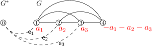
Figure 8. The Cayley embedding of the flow polytope of a graph $G$ is equivalent to the flow polytope of the graph $G^{\star}$ obtained from $G$ by adding a vertex $0$ with edges $(0,i)$ for $i=1,\ldots,n$.

Acknowledgements

We thank Alex Postnikov and Richard Stanley for sharing their insights into triangulating $\mathcal{F}_{G}(1,0,\ldots,0,-1)$, which served as the starting point of our work. We also thank Federico Castillo, Sylvie Corteel, Rafael González D’Léon, Fu Liu and Michele Vergne for helpful comments and suggestions.

Appendix A Examples of canonical subdivisions and Lidskii formulas

Example A.1.

For the graph $G$ with vertices $[3]$ and edges $\{(1,2),(1,2),(2,3),(2,3)\}$ (see Figure 1, left) we have that $({\rm out}_{1},{\rm out}_{2})=(1,1)$. The basic reduction tree for $\mathcal{F}_{G}(1,1,-2)$ is given in Figure 9, left. The Lidskii volume formula (1.1) gives

$${\rm vol}\mathcal{F}_{G}({\bf 1})=\binom{2}{1,1}K_{G}(1-1,1-1,0)+\binom{2}{2,0}K_{G}(2-1,0-1,0)=2\cdot 1+1\cdot 2=4.$$

The first Lidskii lattice point formula (1.2) gives

$$K_{G}(1,1,-2)=\binom{2}{1}\binom{2}{1}K_{G}(0,0,0)+\binom{2}{2}\binom{2}{0}K_{G}(1,-1,0)=4\cdot 1+1\cdot 2=6.$$

Since $({\rm in}_{1},{\rm in}_{2})=(-1,1)$, the second Lidskii lattice point formula 1.3 gives

$$K_{G}(1,1,-2)=\mathchoice{\left(\kern-5.0pt{\binom{2}{1}}\kern-5.0pt\right)}{\bigl{(}\kern-3.00003pt{\binom{2}{1}}\kern-3.00003pt\bigr{)}}{\bigl{(}\kern-3.00003pt{\binom{2}{1}}\kern-3.00003pt\bigr{)}}{\bigl{(}\kern-3.00003pt{\binom{2}{1}}\kern-3.00003pt\bigr{)}}\mathchoice{\left(\kern-5.0pt{\binom{0}{1}}\kern-5.0pt\right)}{\bigl{(}\kern-3.00003pt{\binom{0}{1}}\kern-3.00003pt\bigr{)}}{\bigl{(}\kern-3.00003pt{\binom{0}{1}}\kern-3.00003pt\bigr{)}}{\bigl{(}\kern-3.00003pt{\binom{0}{1}}\kern-3.00003pt\bigr{)}}K_{G}(0,0,0)+\mathchoice{\left(\kern-5.0pt{\binom{2}{2}}\kern-5.0pt\right)}{\bigl{(}\kern-3.00003pt{\binom{2}{2}}\kern-3.00003pt\bigr{)}}{\bigl{(}\kern-3.00003pt{\binom{2}{2}}\kern-3.00003pt\bigr{)}}{\bigl{(}\kern-3.00003pt{\binom{2}{2}}\kern-3.00003pt\bigr{)}}\mathchoice{\left(\kern-5.0pt{\binom{0}{0}}\kern-5.0pt\right)}{\bigl{(}\kern-3.00003pt{\binom{0}{0}}\kern-3.00003pt\bigr{)}}{\bigl{(}\kern-3.00003pt{\binom{0}{0}}\kern-3.00003pt\bigr{)}}{\bigl{(}\kern-3.00003pt{\binom{0}{0}}\kern-3.00003pt\bigr{)}}K_{G}(1,-1,0)=0+3\cdot 2=6.$$

The subdivision yields $K_{G}(1,-1,0)=2$ cells of one type with three lattice points and $K_{G}(0,0,0)=1$ cell of another type with four lattice points. Depending on how the lattice points of the common facets are counted, we obtain the two formulas above. See Figure 9, right.

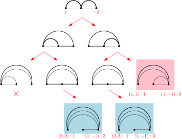
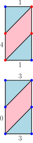
Figure 9. Left: the basic reduction tree for the polytope $\mathcal{F}_{G}(1,1,-2)$ where $G$ has edges $\{(1,2),(1,2),(2,3),(2,3)\}$. Below each leaf $G({\bf m})$, the lattice point contribution of the corresponding cells is given in the form ${\bf v}:K_{G({\bf m})}({\bf v})$ where ${\bf v}={\bf a}-{\bf G({\bf m})}$ and ${\bf v}={\bf a}-{\bf G({\bf m})}^{\prime}$. Right: the canonical subdivision of the polytope given by the reduction tree illustrating (1.2) and (1.3) . The lattice points are colored according to the contribution of each cell.

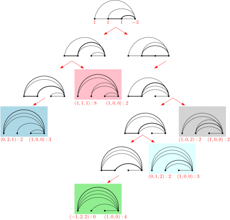
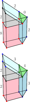
Figure 10. Left: the basic reduction tree for the polytope $\mathcal{F}_{\operatorname{PS}_{3}}(1,1,1,-3)$. Below each leaf $G({\bf m})$, the lattice point contribution of the corresponding cells is given in the form ${\bf v}:K_{G({\bf m})}({\bf v})$ where ${\bf v}={\bf a}-{\bf G({\bf m})}$ and ${\bf v}={\bf a}-{\bf G({\bf m})}^{\prime}$. Right: the canonical subdivision of the polytope given by the reduction tree illustrating (1.2) and (1.3) . The lattice points are colored according to the contribution of each cell.

Example A.2.

For the graph $\operatorname{PS}_{3}$ (see Figure 1, center) we have that $({\rm out}_{1},{\rm out}_{2},{\rm out}_{3})=(1,1,1)$. The basic reduction tree for $\mathcal{F}_{\operatorname{PS}_{3}}(1,1,1,-3)$ is given in Figure 10, left. Since $K_{\operatorname{PS}_{3}}(a,b,c,0)=1$ or $0$, then the Lidskii volume formula (1.1) gives

$${\rm vol}\mathcal{F}_{\operatorname{PS}_{3}}({\bf 1})=\binom{3}{2,0,1}+\binom{3}{1,1,1}+\binom{3}{3,0,0}+\binom{3}{2,1,0}+\binom{3}{1,2,0}=3+6+1+3+3=16.$$

The first Lidskii lattice point formula (1.2) gives

$$K_{\operatorname{PS}_{3}}(1,1,1,-3)=\binom{2}{0}\binom{2}{1}\binom{2}{2}+\binom{2}{1}^{3}+\binom{2}{0}\binom{2}{1}\binom{2}{2}+\binom{2}{0}\binom{2}{1}\binom{2}{2}=2+8+2+2=14.$$

Since $({\rm in}_{1},{\rm in}_{2},{\rm in}_{3})=(-1,0,0)$, the second Lidskii lattice point formula 1.3 gives

(A.1) $$K_{\operatorname{PS}_{3}}(1,1,1,-3)=\mathchoice{\left(\kern-5.0pt{\binom{2}{2}}\kern-5.0pt\right)}{\bigl{(}\kern-3.00003pt{\binom{2}{2}}\kern-3.00003pt\bigr{)}}{\bigl{(}\kern-3.00003pt{\binom{2}{2}}\kern-3.00003pt\bigr{)}}{\bigl{(}\kern-3.00003pt{\binom{2}{2}}\kern-3.00003pt\bigr{)}}\mathchoice{\left(\kern-5.0pt{\binom{1}{0}}\kern-5.0pt\right)}{\bigl{(}\kern-3.00003pt{\binom{1}{0}}\kern-3.00003pt\bigr{)}}{\bigl{(}\kern-3.00003pt{\binom{1}{0}}\kern-3.00003pt\bigr{)}}{\bigl{(}\kern-3.00003pt{\binom{1}{0}}\kern-3.00003pt\bigr{)}}\mathchoice{\left(\kern-5.0pt{\binom{1}{1}}\kern-5.0pt\right)}{\bigl{(}\kern-3.00003pt{\binom{1}{1}}\kern-3.00003pt\bigr{)}}{\bigl{(}\kern-3.00003pt{\binom{1}{1}}\kern-3.00003pt\bigr{)}}{\bigl{(}\kern-3.00003pt{\binom{1}{1}}\kern-3.00003pt\bigr{)}}+\mathchoice{\left(\kern-5.0pt{\binom{2}{1}}\kern-5.0pt\right)}{\bigl{(}\kern-3.00003pt{\binom{2}{1}}\kern-3.00003pt\bigr{)}}{\bigl{(}\kern-3.00003pt{\binom{2}{1}}\kern-3.00003pt\bigr{)}}{\bigl{(}\kern-3.00003pt{\binom{2}{1}}\kern-3.00003pt\bigr{)}}\mathchoice{\left(\kern-5.0pt{\binom{1}{1}}\kern-5.0pt\right)}{\bigl{(}\kern-3.00003pt{\binom{1}{1}}\kern-3.00003pt\bigr{)}}{\bigl{(}\kern-3.00003pt{\binom{1}{1}}\kern-3.00003pt\bigr{)}}{\bigl{(}\kern-3.00003pt{\binom{1}{1}}\kern-3.00003pt\bigr{)}}\mathchoice{\left(\kern-5.0pt{\binom{1}{1}}\kern-5.0pt\right)}{\bigl{(}\kern-3.00003pt{\binom{1}{1}}\kern-3.00003pt\bigr{)}}{\bigl{(}\kern-3.00003pt{\binom{1}{1}}\kern-3.00003pt\bigr{)}}{\bigl{(}\kern-3.00003pt{\binom{1}{1}}\kern-3.00003pt\bigr{)}}+\mathchoice{\left(\kern-5.0pt{\binom{2}{3}}\kern-5.0pt\right)}{\bigl{(}\kern-3.00003pt{\binom{2}{3}}\kern-3.00003pt\bigr{)}}{\bigl{(}\kern-3.00003pt{\binom{2}{3}}\kern-3.00003pt\bigr{)}}{\bigl{(}\kern-3.00003pt{\binom{2}{3}}\kern-3.00003pt\bigr{)}}\mathchoice{\left(\kern-5.0pt{\binom{1}{0}}\kern-5.0pt\right)}{\bigl{(}\kern-3.00003pt{\binom{1}{0}}\kern-3.00003pt\bigr{)}}{\bigl{(}\kern-3.00003pt{\binom{1}{0}}\kern-3.00003pt\bigr{)}}{\bigl{(}\kern-3.00003pt{\binom{1}{0}}\kern-3.00003pt\bigr{)}}\mathchoice{\left(\kern-5.0pt{\binom{1}{0}}\kern-5.0pt\right)}{\bigl{(}\kern-3.00003pt{\binom{1}{0}}\kern-3.00003pt\bigr{)}}{\bigl{(}\kern-3.00003pt{\binom{1}{0}}\kern-3.00003pt\bigr{)}}{\bigl{(}\kern-3.00003pt{\binom{1}{0}}\kern-3.00003pt\bigr{)}}+\\ +\mathchoice{\left(\kern-5.0pt{\binom{2}{2}}\kern-5.0pt\right)}{\bigl{(}\kern-3.00003pt{\binom{2}{2}}\kern-3.00003pt\bigr{)}}{\bigl{(}\kern-3.00003pt{\binom{2}{2}}\kern-3.00003pt\bigr{)}}{\bigl{(}\kern-3.00003pt{\binom{2}{2}}\kern-3.00003pt\bigr{)}}\mathchoice{\left(\kern-5.0pt{\binom{1}{1}}\kern-5.0pt\right)}{\bigl{(}\kern-3.00003pt{\binom{1}{1}}\kern-3.00003pt\bigr{)}}{\bigl{(}\kern-3.00003pt{\binom{1}{1}}\kern-3.00003pt\bigr{)}}{\bigl{(}\kern-3.00003pt{\binom{1}{1}}\kern-3.00003pt\bigr{)}}\mathchoice{\left(\kern-5.0pt{\binom{1}{0}}\kern-5.0pt\right)}{\bigl{(}\kern-3.00003pt{\binom{1}{0}}\kern-3.00003pt\bigr{)}}{\bigl{(}\kern-3.00003pt{\binom{1}{0}}\kern-3.00003pt\bigr{)}}{\bigl{(}\kern-3.00003pt{\binom{1}{0}}\kern-3.00003pt\bigr{)}}+\mathchoice{\left(\kern-5.0pt{\binom{2}{1}}\kern-5.0pt\right)}{\bigl{(}\kern-3.00003pt{\binom{2}{1}}\kern-3.00003pt\bigr{)}}{\bigl{(}\kern-3.00003pt{\binom{2}{1}}\kern-3.00003pt\bigr{)}}{\bigl{(}\kern-3.00003pt{\binom{2}{1}}\kern-3.00003pt\bigr{)}}\mathchoice{\left(\kern-5.0pt{\binom{1}{2}}\kern-5.0pt\right)}{\bigl{(}\kern-3.00003pt{\binom{1}{2}}\kern-3.00003pt\bigr{)}}{\bigl{(}\kern-3.00003pt{\binom{1}{2}}\kern-3.00003pt\bigr{)}}{\bigl{(}\kern-3.00003pt{\binom{1}{2}}\kern-3.00003pt\bigr{)}}\mathchoice{\left(\kern-5.0pt{\binom{1}{0}}\kern-5.0pt\right)}{\bigl{(}\kern-3.00003pt{\binom{1}{0}}\kern-3.00003pt\bigr{)}}{\bigl{(}\kern-3.00003pt{\binom{1}{0}}\kern-3.00003pt\bigr{)}}{\bigl{(}\kern-3.00003pt{\binom{1}{0}}\kern-3.00003pt\bigr{)}}=3+2+4+3+2=14.$$

The subdivision yields five cells of different types. Depending on how the lattice points of the common facets are counted, we obtain the two formulas above. See Figure 10, right.

References

- [1] W. Baldoni and M. Vergne. Kostant partitions functions and flow polytopes. Transform. Groups, 13(3-4):447–469, 2008.
- [2] W. Baldoni-Silva, J. A. De Loera, and M. Vergne. Counting integer flows in networks. Found. Comput. Math., 4:277–314, 2004.
- [3] W. Baldoni-Silva and M. Vergne. Residues formulae for volumes and Ehrhart polynomials of convex polytopes. arXiv:math/0103097, 2001.
- [4] M. Beck and S. Robins. Computing the Continuous Discretely: Integer-Point Enumeration in Polyhedra. Springer-Verlag, 2007.
- [5] C. Benedetti, R. González D’León, C. R. H. Hanusa, P. E. Harris, A. Khare, A. H. Morales, and M. Yip. A combinatorial model for computing volumes of flow polytopes, 2018. arXiv:1801.07684.
- [6] F. Castillo and F. Liu. Berline-Vergne valuation and generalized permutohedra, 2015. Discrete Comput. Geom., accepted. arXiv:1509.07884.
- [7] C.S. Chan, D.P. Robbins, and D.S. Yuen. On the volume of a certain polytope. Experiment. Math., 9(1):91–99, 2000.
- [8] S. Corteel, J.S. Kim, and K. Mészáros. Flow polytopes with catalan volumes. C. R. Math. Acad. Sci. Paris, 355(3):248 – 259, 2017.
- [9] G. Gallo and C. Sodini. Extreme points and adjacency relationship in the flow polytope. Calcolo, 15:277–288, 1978.
- [10] J. Haglund. A polynomial expression for the Hilbert series of the quotient ring of diagonal coinvariants. Adv. Math., 227(5):2092–2106, 2011.
- [11] L. Hille. Quivers, cones and polytopes. Linear Algebra and its Applications, 365:215–237, 2003.
- [12] B. Huber, J. Rambau, and F. Santos. The Cayley trick, lifting subdivisions and the bohnedress theorem on zonotopal tilings. J. Eur. Math. Soc., 2:179–198, 2000.
- [13] B. V. Lidskiĭn . The Kostant function of the system of roots . Funktsional. Anal. i Prilozhen., 18(1):76–77, 1984.
- [14] F. Liu. On positivity of ehrhart polynomials, 2017. arXiv:1711.09962.
- [15] K. Mészáros and A. H. Morales. Flow polytopes of signed graphs and the Kostant partition function. Int. Math. Res. Not. IMRN, 2015:830–871, 2015.
- [16] K. Mészáros, A.H. Morales, and B. Rhoades. The polytope of tesler matrices. Sel. Math. New Ser., 23:425–454, 2017.
- [17] K. Mészáros, A.H. Morales, and J. Striker. On flow polytopes, order polytopes, and certain faces of the alternating sign matrix polytope. arXiv:1510.03357, 2015.
- [18] K. Mészáros, C. Simpson, and Z. Wellner. Flow polytopes of partitions, 2017. arxiv:1707.03100.
- [19] K. Mészáros and A. St. Dizier. From generalized permutahedra to Grothendieck polynomials via flow polytopes. arXiv:1705.02418, 2017.
- [20] W.G. Morris. Constant Term Identities for Finite and Affine Root Systems: Conjectures and Theorems. PhD thesis, University of Wisconsin-Madison, 1982.
- [21] J. Pitman and R.P. Stanley. A polytope related to empirical distributions, plane trees, parking functions, and the associahedron. Discrete Comput. Geom., 4:603–634, 2002.
- [22] A. Postnikov. Permutohedra, associahedra, and beyond. Int. Math. Res. Not. IMRN, 2009:1026–1106, 2009.
- [23] Neil J. A. Sloane. The On-Line Encyclopedia of Integer Sequences. http://oeis.org/.
- [24] R.P. Stanley and A. Postnikov. Acyclic flow polytopes and Kostant’s partition function, 2000. transparencies link.
- [25] B. Sturmfels. On the Newton polytope of the resultant. J. Algebraic Combin., 3:207–236, 1994.
- [26] C. H. Yan. On the enumeration of generalized parking functions. In Proceedings of the 31st Southeastern International Conference on Combinatorics, Graph Theory and Computing (Boca Raton, FL, 2000), volume 147, pages 201–209, 2000.
- [27] C. H. Yan. Generalized parking functions, tree inversions, and multicolored graphs. Adv. Appl. Math., 27:641–670, 2001. Special issue in honor of Dominique Foata’s 65th birthday.
- [28] D. Zeilberger. Proof of a conjecture of Chan, Robbins, and Yuen. Electron. Trans. Numer. Anal., 9:147–148, 1999.
- [29] Y. Zhou, J. Liu, and H. Fu. Leading coefficients of Morris type constant term identities. Adv. in Appl. Math., pages 24–42, 2017.