A New Measurement of the Temperature Density Relation of the IGM From Voigt Profile Fitting

Abstract

We decompose the Lyman-$\alpha$ (Ly$\alpha$) forest of an extensive sample of 75 high signal-to-noise ratio and high-resolution quasar spectra into a collection of Voigt profiles. Absorbers located near caustics in the peculiar velocity field have the smallest Doppler parameters, resulting in a low-$b$ cutoff in the $b$-$N_{\text{HI}}$ distribution set primarily by the thermal state of intergalactic medium (IGM). We fit this cutoff as a function of redshift over the range $2.0\leq z\leq 3.4$, which allows us to measure the evolution of the IGM temperature-density ($T=T_{0}(\rho/\rho_{0})^{\gamma-1}$) relation parameters $T_{0}$ and $\gamma$. We calibrate our measurements against mock Ly$\alpha$ forest data, generated using 26 hydrodynamic simulations with different thermal histories from the THERMAL suite, also encompassing different values of the IGM pressure smoothing scale. We adopt a forward-modeling approach and self-consistently apply the same algorithms to both data and simulations, propagating both statistical and modeling uncertainties via Monte Carlo. The redshift evolution of $T_{0}$ ($\gamma$) shows a suggestive peak (dip) at $z=2.9$ ($z=3$). Our measured evolution of $T_{0}$ and $\gamma$ are generally in good agreement with previous determinations in the literature. Both the peak in the evolution of $T_{0}$ at $z=2.8$, as well as the high temperatures $T_{0}\simeq 15000-20000\,$K that we observe at $2.4<z<3.4$, strongly suggest that a significant episode of heating occurred after the end of H I reionization, which was most likely the cosmic reionization of He II.

1. Introduction

The evolution of the thermal state of the low density intergalactic medium (IGM) provides us with insight into the nature and evolution of the bulk ($\gtrsim 90\%$) of baryonic matter in the Universe (Meiksin 2009; McQuinn 2016). Of special interest are the thermal imprints of cosmic reionization processes that heated the IGM.

The IGM is believed to have undergone two major reheating events. The first is the reionization of hydrogen (H I $\rightarrow$ H II), likely driven by galaxies (Faucher-Giguère et al. 2008a; Robertson et al. 2015) and/or quasars (QSOs, Madau & Haardt 2015; Khaire et al. 2016), which should be completed by redshift $z\sim 6$ (McGreer et al. 2015). The standard picture is that helium is singly ionized (He I $\rightarrow$ He II) during H I reionization, and that the second ionization of Helium (He II $\rightarrow$ He III) occurred later during a He II reionization phase transition powered by the harder radiation emitted by luminous QSOs. This process is expected to be completed by a redshift of around 2.7 (Worseck et al. 2011). These reionization processes are expected to significantly alter the thermal evolution of the IGM.

Long after reionization events which heat the IGM, the thermal properties of the bulk of the intergalactic gas are well described by a tight power law temperature-density relation of the form $T=T_{0}(\rho/\rho_{0})^{\gamma-1}$ (Hui & Gnedin 1997; McQuinn & Upton Sanderbeck 2016), parametrized by the temperature $T_{0}$ at mean density $\rho_{0}$ and an index $\gamma$. This relation comes about naturally when the gas is mainly heated by photoionization and cooled due to cosmic expansion. Therefore, the evolution of $T_{0}$ and $\gamma$ serves as a diagnostic tool to understand reionization phase transitions. Note that during or just after a reionization process, the gas experiences temperature fluctuations (D’Aloisio et al. 2015) that cause this relation to experience scatter or even become multivalued (McQuinn et al. 2009; Compostella et al. 2013).

Although predominantly photoionized, residual H I in the diffuse IGM gives rise to Lyman-$\alpha$ (Ly$\alpha$) absorption, ubiquitously observed toward distant background quasars. This so-called Ly$\alpha$ forest has been established as the premier probe of the IGM and cosmic structure at redshifts $z\lesssim 6$. In the literature, different approaches were used for measuring the parameters of the temperature-density relation of the IGM from Ly$\alpha$ forest absorption. Studies of the statistical properties of the absorption, such as the power-spectrum of the transmitted flux (e.g. Zaldarriaga et al. 2001; Theuns et al. 2002), the average local curvature (Becker et al. 2011; Boera et al. 2014), the flux probability distribution function (e.g. Bolton et al. 2008; Viel et al. 2009; Lee et al. 2015) and wavelet decomposition of the forest (e.g. Lidz et al. 2010; Garzilli et al. 2012) aimed to constrain the thermal state of the IGM.

In this work, we follow the approach used by Schaye et al. (1999); Ricotti et al. (2000) and McDonald et al. (2001) that treats the Ly$\alpha$ forest as a superposition of discrete absorption profiles. This method was suggested by Haehnelt & Steinmetz (1998); Ricotti et al. (2000) and Bryan & Machacek (2000) and is based on the idea that the distribution of Doppler parameters $b$, i.e. line broadening, of Ly$\alpha$ absorption in the IGM at a given redshift, has a sharp cutoff at low values that can be connected to the thermal state of the IGM.

Generally the Doppler parameter $b$ of an absorber is determined by the contributions from its thermal state and kinematic properties. The thermal contribution consists of microscopic random thermal motions in the gas, or thermal broadening, whereas the kinematic contribution, often referred to as turbulent broadening, results from the peculiar velocities in the IGM as well as the differential Hubble flow across the characteristic size of an absorbing cloud, which is set by the so-called pressure smoothing scale $\lambda_{P}$ (Gnedin & Hui 1998; Schaye 2001; Rorai et al. 2013; Kulkarni et al. 2015; Rorai et al. 2017b). If we observe many absorption features, we will occasionally encounter lines from gas clouds which have a line-of-sight velocity component near zero, i.e. the velocity field is close to a caustic (McDonald et al. 2001). As the broadening of these absorbers is dominated by the thermal contribution, this results in a thermal state dependent cutoff in the distribution of Doppler parameters. Note that this cutoff will be subject to scatter due to effects such as fluctuations in temperature and ionizing background. Assuming that the cutoff is primarily set by the thermal state of the gas, its position will be dependent on the gas density due to the temperature-density relation, or in observable terms, the absorption line column density $N_{\text{\text{HI}}}$. This in turn means that there is a correlation between the position of the lower cutoff in the distribution of Doppler parameters as a function of column densities ($b$-$N_{\text{HI}}$ distribution) and the thermal state of the gas. Measuring the position of this cutoff can thus reveal the underlying $T_{0}$ and $\gamma$.

Recently, a measurement of the thermal state of the IGM based on the cutoff of the $b$-$N_{\text{HI}}$ distribution was carried out by Rudie et al. (2012a) using a sample of 15 high-quality QSO sightlines. Using the analytic relations between the cutoff of the $b$-$N_{\text{HI}}$ distribution and the temperature-density relation derived by Schaye et al. (1999), Rudie et al. (2012a) measured a temperature at mean-density $T_{0}=1.94\times 10^{4}\,$K at $z\sim 2.4$ (in a broad redshift bin spanning $2.0<z<2.8$), which was $\sim 9000\,$K higher than the value implied by curvature measurements at $z=2.4$ by Becker et al. (2011). This discrepancy motivated Bolton et al. (2014) to revisit this measurement. Using hydrodynamical simulations, they calibrated the relationship between the $b$-$N_{\text{HI}}$ distribution cutoff and the temperature-density relation. Applying this updated calibration to the Rudie et al. (2012a) $b$-$N_{\text{HI}}$ distribution cutoff measurement, Bolton et al. (2014) determined a lower temperature $T_{0}(z=2.4)=[1.00^{+0.32}_{-0.21}]\times 10^{4}\,$K that is consistent with Becker et al. (2011), and argued that the much higher temperature measured by Rudie et al. (2012a) resulted from incorrect assumptions in the calibration.

In this work we study the $b$-$N_{\text{HI}}$ distribution of an extensive sample of 75 high quality QSO spectra, which allows us to measure the redshift evolution of $T_{0}$ and $\gamma$ over the redshift range $2.0\leq z\leq 3.4$ with a much finer binning $\delta z=0.2$ than previous work. At each redshift we use mock Ly$\alpha$ forest data from 26 hydrodynamic simulations with different thermal histories to calibrate the relationship between the cutoff in the $b$-$N_{\text{HI}}$ distribution and the thermal parameters ($T_{0}$, $\gamma$, $\lambda_{P}$) governing the IGM. The Ly$\alpha$ forest of both the data and the simulations are decomposed into individual absorption lines using the Voigt-profile fitting algorithm VPFIT (Carswell & Webb 2014), and we adopt a forward-modeling approach whereby the same algorithms are self-consistently applied to both data and simulations.

This paper is structured as follows. We introduce our dataset, Voigt-profile, and cutoff fitting procedure in § 2. An overview of our hydrodynamic simulations is given in § 3, where we also introduce the THERMAL (Thermal History and Evolution in Reionization Models of Absorption Lines) suite. In § 4 we discuss how we calibrate our method by applying the same fitting procedures to simulated sightlines. Our final results on the evolution of the thermal state of the IGM at $2<z<3.4$ are presented and discussed in section § 5. We summarize our results in section § 6.

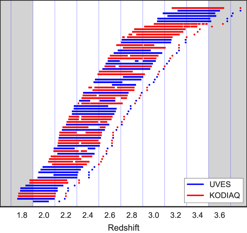
Figure 1.— KODIAQ and UVES Ly$\alpha$ forest sightlines used in this work. The sample is described in § 2. Sightlines from the KODIAQ sample are marked in red and UVES sightlines are marked in blue. The corresponding QSO redshifts are marked as colored points. DLAs and bad regions that were excluded are shown as gaps. The blue vertical lines show the bins that will be used for the cutoff fitting analysis. Gray regions are not used because of lower coverage.

2. Data Processing

2.1. QSO Sample

For this study we used a sample of 75 publicly available QSO spectra with signal-to-noise ratio (SNR) better than 20 per 6 km/s bin and resolution varying between ${\rm FWHM}=3.1$ km/s and 6.3 km/s with a typical value around 6 km/s. This ensures that the Ly$\alpha$ forest is resolved and that we can detect lines with $N_{\text{\text{HI}}}\simeq 10^{12.5}$ cm^-2 at the 3$\sigma$ level (Herbert-Fort et al. 2006). Part of the sample consists of QSO spectra from the Keck Observatory Database of Ionized Absorbers toward QSOs (KODIAQ, Lehner et al. 2014; O’Meara et al. 2016, 2017). The other spectra were acquired with the UV-visual Echelle Spectrograph (Dekker et al. 2000) at the Very Large Telescope (Dall’Aglio et al. 2008).

The KODIAQ sample used in this work consists of 36 QSO sightlines chosen from DR1 and DR2. These QSOs were observed between 1995 and 2012 using the HIRES instrument (High Resolution Echelle Spectrometer: Vogt et al. 1994) on the Keck-I telescope. All the spectra were uniformly reduced and continuum-fitted by eye by the KODIAQ team using the HIRedux code. Spectra with multiple exposures were co-added in order to increase the SNR. The detailed information about the reduction steps is described in O’Meara et al. (2015).

The UVES spectra consist of 38 sightlines from the ESO archive. These objects were chosen to have at least 10 exposures each and complete (or nearly complete) Ly$\alpha$ forest coverage. The data was reduced by Dall’Aglio et al. (2008) using the MIDAS environment ECHELLE/UVES and procedures described in Kim et al. (2004). Each frame was bias and background subtracted. Afterward, the echelle spectra were extracted order by order assuming a Gaussian profile along the spatial direction. The final co-added spectra have exquisite SNR per pixel $\geq 40$ and a resolution of 6 km/s within the Ly$\alpha$ forest. Continua were fitted by Dall’Aglio et al. (2008) using a cubic-spline interpolation method. We used 38 spectra from the 40 available in this sample. One characteristic of the UVES pipeline is that the estimated errors at flux values close to zero is underestimated by a factor of roughly two (Carswell et al. 2014). Therefore Voigt-profile fitting algorithms will struggle to achieve a satisfactory $\chi^{2}$ for these regions. To compensate for this, we used a dedicated tool implemented in RDGEN (Carswell et al. 2014), a front and back-end program for VPFIT. This tool multiplies the error of each pixel with a value that is 1 if the corresponding normalized flux is 1 and 2 if the normalized flux is 0. For this purpose we used the default parametrization from RDGEN.

The region of the spectra used for fitting lies between 1050 Å and 1180 Å rest-frame inside the Ly$\alpha$ forest. This region was chosen to avoid proximity effects, i.e. regions affected by the local QSO radiation rather than the metagalactic UV-Background. This choice is consistent with studies by Palanque-Delabrouille et al. (2013) and Walther et al. (2018).

For a complete list of the spectra analyzed in this work and the essential information about them, refer to Table 1. The chunks of spectra used are plotted in Figure 1 and colored based on the dataset they belong to. Our analysis of the thermal state of the IGM will be done in redshift bins of size $\delta z=0.2$, indicated with vertical blue lines. We discuss the effects of continuum misplacement in our data in the appendix A.

Table 1QSO spectra used in this work. The signal-to-noise value refers to the median value inside the Ly$\alpha$ forest.

Object ID	$z_{qso}$	$SNR/6$ kms-1	Sample
HE1341-1020	2.137	58	UVES
Q0122-380	2.192	56	UVES
J122824+312837	2.2	87	KODIAQ
J110610+640009	2.203	59	KODIAQ
PKS1448-232	2.222	57	UVES
PKS0237-23	2.224	102	UVES
HE0001-2340	2.278	66	UVES
J162645+642655	2.32	104	KODIAQ
J141906+592312	2.321	37	KODIAQ
Q0109-3518	2.406	70	UVES
HE1122-1648	2.407	172	UVES
HE2217-2818	2.414	94	UVES
Q0329-385	2.437	58	UVES
HE1158-1843	2.459	67	UVES
J005814+011530	2.495	36	KODIAQ
J162548+264658	2.518	44	KODIAQ
J121117+042222	2.526	34	KODIAQ
J101723-204658	2.545	70	KODIAQ
Q2206-1958	2.567	75	UVES
J234628+124859	2.573	75	KODIAQ
Q1232+0815	2.575	46	UVES
HE1347-2457	2.615	62	UVES
J101155+294141	2.62	130	KODIAQ
J082107+310751	2.625	64	KODIAQ
HS1140+2711	2.628	89	UVES
J121930+494052	2.633	90	KODIAQ
J143500+535953	2.635	65	KODIAQ
Q0453-423	2.663	78	UVES
J144453+291905	2.669	134	KODIAQ
PKS0329-255	2.705	48	UVES
J081240+320808	2.712	49	KODIAQ
J014516-094517A	2.73	77	KODIAQ
J170100+641209	2.735	82	KODIAQ
Q1151+068	2.758	49	UVES
Q0002-422	2.768	75	UVES
HE0151-4326	2.787	98	UVES
Q0913+0715	2.788	54	UVES
J155152+191104	2.83	30	KODIAQ
Q1409+095	2.843	25	UVES
Q0119+1432	2.87	33	KODIAQ
J012156+144820	2.87	55	KODIAQ
Q0805+046	2.877	27	KODIAQ
HE2347-4342	2.886	152	UVES
J143316+313126	2.94	54	KODIAQ
J134544+262506	2.941	35	KODIAQ
Q1223+178	2.955	33	UVES
Q0216+08	2.996	37	UVES
HE2243-6031	3.011	119	UVES
CTQ247	3.026	69	UVES
J073621+651313	3.038	26	KODIAQ
J194455+770552	3.051	30	KODIAQ
HE0940-1050	3.089	70	UVES
J120917+113830	3.105	31	KODIAQ
Q0420-388	3.12	116	UVES
CTQ460	3.141	41	UVES
J114308+113830	3.146	32	KODIAQ
J102009+104002	3.168	36	KODIAQ
Q2139-4434	3.208	31	UVES
Q0347-3819	3.229	84	UVES
J1201+0116	3.233	30	KODIAQ
J080117+521034	3.236	43	KODIAQ
PKS2126-158	3.285	64	UVES
Q1209+0919	3.291	30	UVES
J095852+120245	3.298	45	KODIAQ
J025905+001126	3.365	26	KODIAQ
Q2355+0108	3.4	58	KODIAQ
J173352+540030	3.425	57	KODIAQ
J144516+095836	3.53	25	KODIAQ
J142438+225600	3.63	29	KODIAQ
Q0055-269	3.665	76	UVES
Q1249-0159	3.668	70	UVES
Q1621-0042	3.708	78	UVES
Q1317-0507	3.719	42	UVES
PKS2000-330	3.786	151	UVES
J193957-100241	3.787	66	KODIAQ

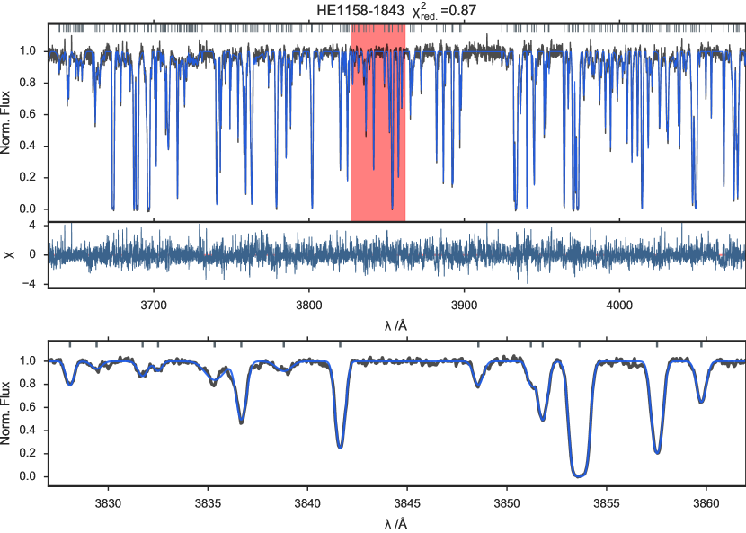
Figure 2.— The resulting VP-fit of the Ly$\alpha$ forest of the QSO HE1158-1843 at $z\simeq 2.46$ from the UVES sample. Upper panel: The original spectrum (black line) is well described by the superposition of Voigt-profiles fitted by VPFIT (blue line). The position of individual lines is shown by gray rugs in the upper part of the panel. Underneath we plot the resulting $\chi=(F_{\text{spec}}-F_{\text{fit}})/\sigma_{F_{\text{fit}}}$ as a measure for the goodness of the fit. Lower Panel: Zoom in of the area marked in red in the upper panel.

2.2. Voigt-Profile Fitting

Voigt-profiles are fitted to our data using VPFIT version 10.2 (Carswell & Webb 2014). We wrote a fully automated set of wrapper routines that prepares the spectra for the fitting procedure and controls VPFIT with the help of the VPFIT front-end/back-end programs RDGEN and AUTOVPIN. These are used to generate initial guesses for the absorption line parameters, output tables, and determine which segments to fit separately. For each segment VPFIT looks for the best fitting superposition of Voigt-profiles that describes a given spectrum. Each line is described by three parameters: line redshift $z_{\text{abs}}$, Doppler parameter $b$, and column density $N_{\text{\text{HI}}}$ corresponding to the chosen absorbing gas transition (here hydrogen Ly-$\alpha$). The parameter space chosen for VPFIT to look for lines was set to go from 1 to 300 km/s in $b$ and 11.5 to 16.0 in $\log(N_{\text{HI}}$/cm^-2). VPFIT then varies these parameters and searches for a solution that minimizes the $\chi^{2}$. If the $\chi^{2}$ is not satisfying, then it will add lines until the fit converges or no longer improves. In order to minimize computational time, this fitting procedure is done in different segments of the spectra at a time. It is possible to automatically find regions that are between sections of the spectra where the flux meets the continuum, i.e. no absorption, and fit them separately. The fitted spectrum is then put together as a collection of line parameters.

Damped Ly$\alpha$ systems (DLAs), i.e. Ly$\alpha$ absorbers with $N_{\text{HI}}\gtrsim 10^{20}$cm^-2, were identified by eye and are excluded from our analysis. The DLAs were chosen to enclose a region between the two points where the damping wings reach the QSO continuum within the flux error. Additionally, regions larger than 30 pixels previously masked in the data (bad pixels, gaps, etc.) were also excluded. We simply cut out the regions in which these rejections apply and feed the usable data segments into VPFIT separately.

In order to avoid chopping our spectra into too many small segments, small regions ($\leq$ 30 pixels) that were previously masked in the data were cubically interpolated. These pixels were given a flux error of a 100 times the continuum so the Voigt-profile fitting procedure is not influenced.

One complication is that VPFIT often has difficulty fitting the boundaries of spectra. To solve this problem we artificially make the chunks longer. For this purpose we append a mirrored version of the first quarter of the spectra to the beginning of it. We do the same with the last quarter to the end of the spectrum. These regions and the line fits within them are later ignored. This method ensures that the unreliable fits at the boundaries happen in an artificial environment that will not be used. The disadvantage is that the spectrum that VPFIT receives is 50% longer than the original and will therefore need more time to be processed.

An example of the VP-fitted spectrum of an UVES sightline is shown in Figure 2.

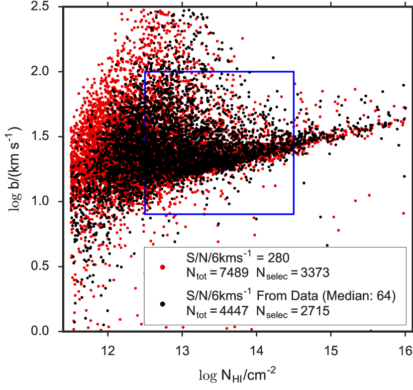
Figure 3.— Simulated $b$-$N_{\text{HI}}$ distributions at z=2.4 with different SNR applied to lines-of-sight. The $b$-$N_{\text{HI}}$ distributions were generated by VP-fitting the same 80 mock skewers from collisionless simulations, adding noise and resolution effects. The $b$-$N_{\text{HI}}$ distribution based on high SNR skewers (red) has a higher number of fitted lines than the distribution created based on the SNR distribution of our data at this redshift (black). The high SNR distribution is more complete at low $\log N_{\text{HI}}$ high $\log b$. The blue box shows the region chosen for our further analysis. The completeness is comparable within this box. The thermal parameters used in these mocks are $\gamma=1.5$, $\log T_{0}/\text{K}=4.04$ and the smoothing length is $\lambda_{P}=47\,$kpc.

2.3. The $b$-$N_{\text{HI}}$ Distribution

The output of VPFIT can be used to generate a $\log b$ vs. $\log(N_{\text{HI}}/$cm^-2) diagram ($b$-$N_{\text{HI}}$ distribution). Note that for a comparatively small number of lines, VPFIT outputs the errors as being zero, nan or “*******”. When generating diagrams, we exclude these lines, because they normally appear in blended regions and noisy parts of the spectra.

In order to illustrate the effect of SNR on the $b$-$N_{\text{HI}}$ distribution, we generate 2 $b$-$N_{\text{HI}}$ distributions by Voigt-profile fitting mock Ly$\alpha$ forest absorption spectra at $z=2.4$ with different SNR applied to them. For this simple exercise we used mock Ly$\alpha$ forest spectra based on collisionless dark matter only simulations. The resulting distributions are shown in Figure 3. In one case (red) we added a constant and extremely high SNR/6 kms^-1 of 280, while in the other case (black) a SNR based on the data at $z=2.4$ (with a median of SNR/6 kms^-1=64) was applied. Some of the features are identical, especially the existence and position of a cutoff at $\log N_{\text{HI}}/\text{\text{cm}${}^{-2}$}>12.5$ and $\log b/$(kms^-1) $\sim 1.2$. The main difference is that the high SNR distribution is more complete towards low $\log N_{\text{HI}}$ and high $\log b$ values. At column densities $\log N_{\text{HI}}/\text{\text{cm}${}^{-2}$}>12.5$ and Doppler parameters $8\,\text{km/s}\leq b\leq 100\,\text{km/s}$ both distributions are similarly populated. Therefore for the cutoff fitting procedure we will only use the part of the $b$-$N_{\text{HI}}$ distribution with $\log N_{\text{HI}}/\text{\text{cm}${}^{-2}$}>12.5$, which is the convention adopted in Schaye et al. (2000) and Rudie et al. (2012a). We also want to avoid saturated absorbers, i.e. $N_{\text{HI}}>10^{14.5}$cm^-2, to make sure that we are using only well constrained column densities. Lines with $b<8$ km/s are excluded because these are most likely metal line contaminants or VPFIT artifacts. Lines with $b>100$ km/s are excluded as well, because the turbulent broadening component dominates over thermal broadening for such broad lines. This is the same convention used in Rudie et al. (2012a) and is shown as a blue box.

Additionally, we decided, based on Schaye et al. (1999), to exclude points that have relative errors worse than 50% in $b$ or $N_{\text{HI}}$. This is done to avoid using badly constrained absorbers in the procedure, as they lie mostly in the part of the $b$-$N_{\text{HI}}$ distribution that is affected by the SNR effects described in Figure 3 at high-$b$ and low-$N_{\text{HI}}$. Lines with $b<11$km/s, i.e. below the low-$b$ envelope of the distribution are generally not excluded by this procedure.

2.3.1 Metal masking

It is well known that narrow absorption lines arising from ionic metal line transitions contaminate the Ly$\alpha$ forest, and will particularly impact the lower $b\lesssim 10\,$km/s region of the $b$-$N_{\text{HI}}$ distribution if treated as Ly$\alpha$ absorption, thus possibly making the determination of the position of the lower envelope of the $b$-$N_{\text{HI}}$ distribution ambiguous. To address this issue we remove lines from our sample that are potentially of metal origin.

However, narrow absorption lines are not necessarily metal line contaminants. We visually inspected the absorption lines with $b\lesssim 10$km/s in every sightline and found that although many could be identified as metal lines wrongly fit as Ly$\alpha$ absorption, a comparable number are simply narrow components that VPFIT adds to obtain the best fit to complex Ly$\alpha$ absorption features. The latter are a property of the fitting procedure and should not be excluded, as they are present in both data and the simulated spectra that we use to conduct our analysis. In order to diminish the problem of metal line contamination we remove metal line contaminants combining automated and visual identification methods, which we describe in detail below.

Metals are typically associated either with strong HI absorption, or they can be identified via associations with other ionic metal line transitions. Therefore, we identified DLAs based on the damping wings of the absorption profiles and determined their redshifts with the help of associated metal absorption redwards of the Ly$\alpha$ emission peak of the QSO in question. The redshifts of other strong metal absorption systems not associated to a DLA within the data coverage or significantly shifted from a DLA are determined by searching for typical doublet absorption systems (mostly Si IV, C IV, Mg II, Al III) redwards of the QSO’s Ly$\alpha$ emission peak. In both cases the doublets are identified based on their characteristic $\Delta\lambda$ (see Table 2.3.1) and line-ratios.

Additionally, we selected lines with Doppler parameters $b<11\,\text{km/s}\times(N_{\text{HI}}/10^{12.95}{\text{cm}^{-2}})^{(1.15-1)}$ in the $b$-$N_{\text{HI}}$ distributions (red line in Figure 4) and traced them back to their positions in the spectra. This relation was chosen based on visual inspection of the $b$-$N_{\text{HI}}$ distributions at all redshift bins and chosen to lie underneath the lower envelope of the full dataset. We checked if we could find a match for different doublet ionic transitions within the Ly$\alpha$ forest for these lines (typically Si IV, C IV and Mg II) by testing for the $\Delta\lambda$ and line-ratios. We then confirmed them by finding corresponding absorption of other metals redwards of the Ly$\alpha$ emission peak of the QSOs at the same redshift. We then tested if the remaining lines below the lower envelope of the $b$-$N_{\text{HI}}$ distribution were any of the metal transitions listed in Table 2.3.1 by checking if other metal transitions and Ly$\alpha$ absorption appear at the same redshift. The redshifts of systems positively identified as a metal line absorption with this method are stored. Candidate metal line absorbers only identified via a single metal feature or a doubtful doublet feature, i.e. with one of the components possibly within a superposition of absorption features, were not considered as secure metal identification and thus are not masked. Given that it targets the absorbers found during the VP-fitting procedure, this method has the advantage that it allows us to identify metal absorbers within the Ly$\alpha$ forest region.

To further refine our metal line search, we used a semi-automated procedure to identify high column density ($N_{\textrm{HI}}/\text{\text{cm}${}^{-2}$}\simeq$15) H I absorbers in our sample as these might also be associated with strong metal absorption. This algorithm identifies groups of pixels in a spectrum that have flux at the relative positions of Ly$\alpha$, $\beta$, $\gamma$ and higher orders (if available) within one sigma threshold of zero. The detected systems are then visually compared to theoretical line profiles of absorbers with $\log(N_{\textrm{HI}}/\text{\text{cm}${}^{-2}$})=15,\leavevmode\nobreak\ 16,\leavevmode\nobreak\ 17$ in Ly$\alpha$ and higher transitions up to Ly$\gamma$. If the absorption profile resembles that of a strong absorber, the redshift of the absorption system is saved. If the absorption was stronger than the $\log(N_{\textrm{HI}}/\text{\text{cm}${}^{-2}$})=15$ profile, then associated metals were masked (not the H I absorption).

Once we have the redshifts of the metal absorption systems, we create a mask based on the relative wavelength positions of the metal transitions listed in Table 2.3.1. All listed transitions are used for generating masks, except for the systems identified with the automated method, i.e. the ones associated with $\log(N_{\textrm{HI}}/\text{\text{cm}${}^{-2}$})\geq 15$. In this case we opted for a reduced list of strong ionic transitions (indicated in Table 2.3.1). In case the position of any line from the VPFIT output falls within $\pm$30km/s from a potential metal line, it is removed from the line list. Additionally, Galactic CaII (3968Å, 3933Å) absorption was masked with a $\pm 150\,$km/s window.

Figure 4 shows normalized contours for all lines rejected using the narrow line rejection method described above (gray contour lines) and the lines that were kept (red filled contours) in our sample. We also show the fraction of points rejected in different regions of the $b$-$N_{\text{HI}}$ distribution. Our metal line filtering approach will inevitably also filter out lines that are genuine Ly$\alpha$ absorption because of the window size of 30 km/s used in the narrow line rejection, removing 24% of the absorbers that are not narrow. This effect is visible in the overlap of rejected and accepted absorbers at $\log b>11\,$km/s. Nevertheless, we identified and removed $65\%$ of all absorbers in our dataset that are likely to be metal line contamination within our cutoff fitting range.

Table 2List of masked metal transitions.

Absorber	$\lambda_{\mathrm{rest}}/\AA$	Absorber	$\lambda_{\mathrm{rest}}/\AA$
O VI	1031.9261	Si IV	1402.770
C II	1036.3367	Si II	1526.7066
O VI	1037.6167	C IV	1548.195
N II	1083.990	C IV	1550.770
Fe III	1122.526	Fe II	1608.4511
Fe II	1144.9379	Al II	1670.7874
Si II	1190.4158	Al III	1854.7164
Si II	1193.2897	Al III	1862.7895
N I	1200.7098	Fe II	2344.214
Si III	1206.500	Fe II	2374.4612
N V	1238.821	Fe II	2382.765
N V	1242.804	Fe II	2586.6500
Si II	1260.4221	Fe II	2600.1729
O I	1302.1685	Mg II	2796.352
Si II	1304.3702	Mg II	2803.531
C II	1334.5323	Mg I	2852.9642
C II*	1335.7077	Ca I	3934.777
Si IV	1393.755	Ca I

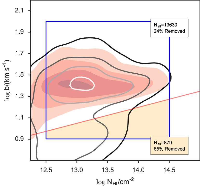
Figure 4.— All lines in our QSO sample divided into two groups: the ones that were rejected using our narrow line rejection methods (gray contour lines) and the ones that were kept and will be used for further analysis (red filled contours). For the sake of visibility, we plot the two clouds of points as continuous and normalized density distributions, calculated using a kernel density estimation method. The lines correspond to 5 equally spaced bins in density, i.e. the 80, 60, 40 and 20 percentiles of the corresponding density distributions. The blue square corresponds to our cutoff fitting region. The solid red line broadly represents the dividing line between the bulks of the distributions of broad and narrow lines with with $b<11\,\text{km/s}\times(N_{\text{HI}}/10^{12.95}{\text{cm}^{-2}})^{(1.15-1)}$. To illustrate the region mostly affected by narrow lines in our cutoff fitting procedure, we show the orange region. The fact that the red contours have little density below the red line, indicates that our metal rejection methods exclude most of the contamination. This happens at the cost of fraction of the usable data, i.e. the lines in the gray contours that are not narrow. The total (both rejected and accepted together) number of lines $N_{\text{all}}$ within the blue square is shown above and below the solid red line, as well as the percentage of these lines that were rejected as possible metal absorbers.

2.3.2 Narrow Line Rejection

Even after a careful metal line masking procedure, many unidentified narrow lines still remain in our line lists. These are narrow lines in blends and unidentified metal lines.

One option to avoid these lines is by simultaneously fitting absorption profiles in the Lyman-$\beta$ (or higher transitions) forest, as in Rudie et al. (2012a). While this approach may deliver cleaner $b$-$N_{\text{HI}}$ distributions, reproducing the same procedure applied to the data on simulations is very complicated as it requires that one models higher-order Lyman series absorption as well. Furthermore, the Rudie et al. (2012a) selection of lines was not completely automated, and decisions about what lines to keep were made by eye, which cannot be automatically applied to simulations (see Rudie et al. 2012b, for more details). Therefore, in this work we chose to use only the Ly$\alpha$ forest region.

Since there is no obvious way of filtering the remaining narrow lines, we need to come up with a rejection mechanism to filter them and diminish their impact on our cut-off fitting procedure. To account for this problem Schaye et al. (1999) removed all the points in the $b$-$N_{\text{HI}}$ distribution where the best fitting Hui-Rutledge function to the $b$-distribution dropped below $10^{-4}$ at the low $b$ end. In Rudie et al. (2012a), the authors applied a more sophisticated algorithm that iteratively removes points from the $b$ distributions (with $b<40$ km/s) in $\log N_{\text{HI}}$ bins in case they are more than $2\sigma$ away from the mean.

In this work we approach this problem in a very similar way as in Rudie et al. (2012a) Our rejection algorithm bins the points within $12.5\leq\log(N_{\text{HI}}$/cm^-2)$\leq 14.5$ into 6 bins of equal size in $\log(N_{\text{HI}}$/cm^-2). Only points with $b$ $<$ 45 km/s are used for the 2$\sigma$ rejection process. For each of the aforementioned bins we compute the mean and the variance of $b$. Points below $2\sigma$ of the mean are excluded. This procedure is iterated until no points are excluded. Finally, after the last iteration, we fit a line to the $\log b_{2\sigma}$ values of each $\log(N_{\text{HI}})$ bin. Once the position of this line is determined, we exclude all points below it from the original sample. We have tested this algorithm for the effect of varying the $\sigma$ threshold and found that the end results are consistent with each other within the errors.

In Figure 5 we show a histogram with the number of absorbers in every redshift bin of our data sample and the effects of rejections. Here we see that the $2\sigma$ rejection excludes a relatively small fraction of the points in the $b$-$N_{\text{HI}}$ distribution.

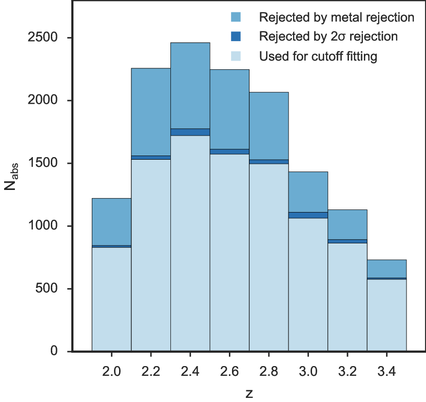
Figure 5.— Number of absorbers fitted by VPFIT per $\delta z$ bin. The histogram shows the number of lines within the cutoff fitting range after metal lines rejection and the 2$\sigma$ rejection were applied.

Figure 6.— The $b$-$N_{\text{HI}}$ distributions in the redshift range $1.9\leq z<3.5$ in $\delta z=0.2$ bins (corresponding to the sightlines in Figure 1). The best cutoff fits (red) and 2$\sigma$-rejection (black) lines are overplotted. The shaded blue region represents the 68% confidence region of the fits to bootstrap realizations at every column density. The corresponding $N_{\text{HI,0}}$ is plotted as an open red point and is calculated by plugging in the bin center redshift into eqn. 11. These measurements allow us to access the evolution of $b_{0}$ and $\Gamma$ as a function of redshift.

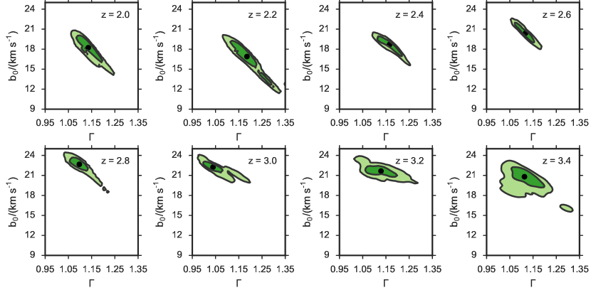
Figure 7.— Resulting $p(b_{0},\Gamma)$ pdfs generated from cutoff fits to 2000 bootstrap realizations of the $b$-$N_{\text{HI}}$ distributions at each redshift. The 68% confidence levels are plotted in dark green and 95% in light green. The black point corresponds to the median of the marginal distributions of $b_{0}$ and $\Gamma$.

2.3.3 Fitting the Cutoff in the $b$-$N_{\rm HI}$ Distribution

Once we have the $b$-$N_{\text{HI}}$ distributions, we want to determine where the thermal state sensitive cutoff is positioned. The position of the cutoff is calculated using our version of an iterative fitting procedure first introduced by Schaye et al. (1999) and also used in Rudie et al. (2012a). The function used for the cutoff of the $b$-$N_{\text{HI}}$ distribution is given by

$$\log b_{\text{th}}=\log b_{0}+(\Gamma-1)\log(N_{\text{HI}}/N_{\text{HI,0}}).$$ (1)

where $b_{0}$ is the minimal broadening value at column density $N_{\text{HI,0}}$ and $\Gamma$ is the index of this power law relation.

Although the value of $N_{\text{HI,0}}$ is essentially just a normalization, as we will motivate further in our discussion of the estimation of $N_{\text{HI,0}}$ in § 4.2, it is convenient to choose it so that it corresponds to the column density of a typical absorber at the mean density of the IGM. Schaye (2001) showed that an absorber corresponding to an overdensity $\Delta=\rho/\rho_{0}$ with size of order of the IGM Jeans scale will have a column density

$$N_{\text{HI}}\simeq 10^{13.23}\text{cm}^{-2}\Delta^{3/2}\frac{T_{4}^{-0.22}}{\Gamma_{\text{ion,HI}}}\left(\frac{1+z}{3.4}\right)^{9/2},$$ (2)

where $\Gamma_{\text{ion,HI}}$ is the photoionization rate of H I and $T_{4}$ is the temperature of the absorbing gas in units of $10^{4}\,K$. We compute $N_{\text{HI,0}}=N_{\rm HI}(\Delta=1)$ at each redshift using this eqn. and discuss how it impacts our calibration in § 4.2.

In our iterative cutoff fitting procedure, we fit eqn. (1) to points in the $b$-$N_{\text{HI}}$ distribution using a least-squares minimization algorithm which takes into account the errors reported by VPFIT. Note that previous works (Schaye et al. 1999; Bolton et al. 2014; Rorai et al. 2018) have used a least absolute deviation method for fitting. For a method comparison and discussion see Appendix B.

The first step of the cutoff fitting procedure is to fit eqn. (1) to all points that are within $10^{12.5}\text{\text{cm}${}^{-2}${}}<N_{\text{HI}}<10^{14.5}\text{\text{cm}${}^{-2}${}}$ and $8\ \text{km/s}<b<100\ \text{km/s}$. The first iteration results in a fit that falls somewhere close to the mean of the distribution. Then we compute the mean absolute deviation in terms of $\log b$ of all $N$ absorbers with respect to the first fit:

$$\left<\left|\delta\log b\right|\right>=\frac{1}{N}\sum^{N}_{i}|\log b_{i}-\log b_{\text{th}}(N_{\text{HI},i})|.$$ (3)

Notice that this takes the deviations both above and below the fit into account. All the points that have a Doppler parameter with $\log b>\log b_{\text{th}}+\left<\left|\delta\log b\right|\right>$ are excluded in the next iteration. This process is repeated without the points excluded in the previous iteration until no points are more than one absolute mean deviation above the fit, which defines convergence. After convergence, the absorbers that are more than one mean deviation below the last fit are excluded. The remaining points are used for the final fit.

2.4. Data cutoff fitting results

Figure 6 shows the $\log b(z)$-$\log N_{\text{\text{HI}}}{}(z)$ distributions resulting from the VP-fitting procedure and the respective cutoff fits (red) and 2$\sigma$ rejection lines (black). The values of $N_{\text{HI,0}}$ chosen for each cutoff fit are calculated using eqn. (11) at the central redshift of each bin. Their values are plotted as open red circles. We determine the uncertainty in the cutoff fit parameters via a bootstrap procedure. For this purpose, we generate the PDF $p(b_{0},\Gamma)$ by bootstrapping the cutoff fitting procedure 2000 times using random realizations of the $b$-$N_{\text{HI}}$ distribution points with replacement. This results in a list with 2000 pairs of $(b_{0},\Gamma)$. The 68% confidence region of the bootstrap cutoff fits is shown in light blue. For illustration, a kernel density estimation of $p(b_{0},\Gamma)$ at every redshift is shown in Figure 7. The anti-correlation between $b_{0}$ and $\Gamma$ is evident.

3. Simulations

In this section we describe how we generate Ly$\alpha$ forest mock spectra from Nyx hydrodynamic simulations (Almgren et al. 2013; Lukić et al. 2015) with different combinations of underlying thermal parameters $T_{0}$, $\gamma$ and $\lambda_{P}$. We apply the exact same Voigt-profile and $b$-$N_{\text{HI}}$ distribution cutoff fitting algorithms as for the data in order to calibrate the relations between the parameters that describe the cutoff ($b_{0}$ and $\Gamma$) and the thermal parameters ($T_{0}$ and $\gamma$) while marginalizing over different values of the pressure smoothing scale $\lambda_{P}$.

The evolution of dark matter in Nyx is calculated by treating dark matter particles as self gravitating Lagrangian particles, while baryons are treated as an ideal gas on a uniform Cartesian grid. Nyx uses a second-order accurate piecewise parabolic method (PPM) to solve for the Eulerian gas dynamics equations, which accurately captures shock waves. For more details on the numerical methods and scaling behavior tests, see Almgren et al. (2013) and Lukić et al. (2015). These simulations also include the physical processes needed to model the Ly$\alpha$ forest. The gas is assumed to be of primordial composition with Hydrogen and Helium contributing 75% and 25% by mass. All relevant atomic cooling processes, as well as UV photo-heating, are modeled under assumption of ionization equilibrium. Inverse Compton cooling off the microwave background is also taken into account. We used the updated recombination, cooling, collision ionization and dielectric recombination rates from Lukić et al. (2015).

As is standard in hydrodynamical simulations that model the Ly$\alpha$ forest forest, all cells are assumed to be optically thin to radiation. Radiative feedback is accounted for via a spatially uniform, but time-varying ultraviolet background (UVB) radiation field, input to the code as a list of photoionization and photoheating rates that vary with redshift (e.g. Katz et al. 1992). We have created a grid of models that explore very different thermal histories combining different methodologies. First we have used the approach presented in Oñorbe et al. (2017), which allows us to vary the timing and duration of reionization, and its associated heat injection, enabling us to simulate a diverse range of reionization histories. This method allows us to create the H I, He I and He II photoionization and photoheating rates, which are inputs to the Nyx code, by volume averaging the photoionization and energy equations. We direct the reader to Oñorbe et al. (2017) for the details of this method. On top of this we also use the methodology first introduced by Bryan & Machacek (2000) of rescaling the photoheating rates by factor, $A$, as well as making the heating depend on density according to $\Delta^{B}$ (Becker et al. 2011), with $B$ being also a free parameter. Combining all these approaches allows us to built a large set of different thermal histories and widely explore the thermal parameter space of $T_{0}$, $\gamma$ and $\lambda_{P}$ at different redshifts.

The THERMAL Suite (Thermal History and Evolution in Reionization Models of Absorption Lines) consists on more than 60 Nyx hydrodynamical simulations with different thermal histories and $L_{\text{box}}=20\,\text{Mpc}/h$ and $1024^{3}$ cells based on a Planck Collaboration et al. (2014) cosmology $\Omega_{m}=0.3192$, $\Omega_{\Lambda}=0.6808$, $\Omega_{b}=0.04964$, $h=0.6704$, $n_{s}=0.96$, $\sigma_{8}=0.826$. As shown in Lukić et al. (2015) for a Haardt & Madau (2012) model, simulations of this box size and larger ones result in nearly the same distribution of column densities and Doppler parameters for the range of these parameters used in this work. The suite also has some extra simulations with different cosmological seeds, box size, resolution elements and/or cosmology to provide a reliable test bench for convergence and systematics associated with different observables. For all simulations we have data for every $\Delta z=0.2$ from $z=6.0$ down to $z=1.6$, as well as at $z=1.0$, $z=0.5$ and $z=0.2$.

In this work we use a subset of 26 simulations from the THERMAL Suite that were selected to optimize the space of thermal parameters (described below) within the redshift range in which we are interested $2.0<z<3.4$. The thermal parameters $T_{0}$ and $\gamma$ are extracted from the simulations by fitting a power law $T$-$\rho$ relation to the distribution of gas cells as described in Lukić et al. (2015). In order to determine the pressure smoothing scale $\lambda_{P}$, the cutoff in the power spectrum of the real-space Ly$\alpha$ flux $F_{\mathrm{real}}$ is fitted. $F_{\mathrm{real}}$ is the flux each position in the simulation would have given it’s temperature and density, but neglecting redshift space effects (see Kulkarni et al. 2015).

3.1. Skewer Generation

In order to model lines-of-sight through the IGM, we extract a random subset of hydrogen density skewers from our simulations that run parallel to the box axes. These are transformed into Ly$\alpha$ optical depth skewers (we refer to Lukić et al. 2015 for specific details about these calculations). The corresponding flux skewer $F$, i.e. a transmission spectrum along the line-of-sight, is calculated from the optical depth using $F=\exp(-A_{r}\,\tau)$. Here we introduce a scaling factor $A_{r}$ that allows us to match our lines-of-sight to observed mean flux values. This re-scaling of the optical depth accounts for the lack of knowledge of the precise value of the metagalactic ionizing background photoionization rate. To this end we choose $A_{r}$ so that we match the mean-flux evolution shown in Oñorbe et al. (2017), which is a fit at $0.2<z<5.85$ based on measurements of various authors (Fan et al. 2006; Kim et al. 2007; Faucher-Giguère et al. 2008a; Becker et al. 2013). Given the extremely high precision with which the mean flux has been measured by these authors, we do not consider the impact of uncertainties in the re-scaling value $A_{r}$. A discussion about the effects of mean flux rescaling in the models on our results is presented in the Appendix C.

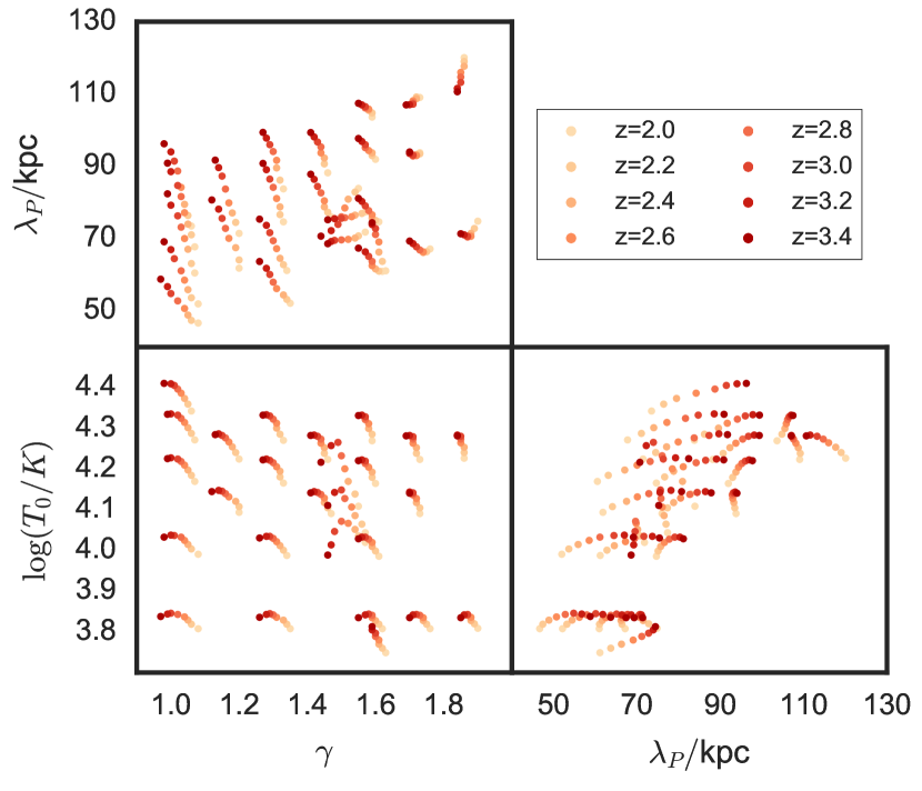
Figure 8.— Combinations of parameters $T_{0}$, $\gamma$ and $\lambda_{P}$ used for generating model skewers used in the calibration process. This grid was generated at redshifts 2.0 to 3.4 in $\delta z=0.2$ steps to match our data. The evolution of the grid with redshift reflects the thermal history of the Nyx simulations chosen.

3.2. Thermal Parameter Grid

We used simulation snapshots at 8 different redshifts from $z=2.0$ to $3.4$ in $\delta z=0.2$ steps, which matches the redshift distribution of our data. We then generate 150 skewers for $2.0\leq z\leq 3.0$ and 75 skewers for $3.2\leq z\leq 3.4$ for each of the 26 combinations of thermal parameters ($T_{0}$, $\gamma$ and $\lambda_{P}$). Figure 8 shows the distribution of thermal parameters chosen. We chose to model the thermal parameters on an irregular grid covering the range $47\,\text{kpc}<\lambda_{P}<120\,\text{kpc}$, which is well within the range of measurements by Rorai et al. (2013, 2017b) of $40\,\text{kpc}<\lambda_{P}<130\,\text{kpc}$ for $2<z<3.6$. For this comparison we scaled the measurements of Rorai et al. (2013, 2017b) to match $\lambda_{P}$ as defined in Kulkarni et al. (2015). The grid of parameters of the temperature-density relation covers $0.97<\gamma<1.9$ and $5600\ \text{K}<T_{0}<25700\ \text{K}$.

3.3. Forward Modeling Noise and Resolution

To create mock spectra we add the effects of resolution and noise, both based on our data, to our simulated skewers. We mimic instrumental resolution by convolving the skewers with a Gaussian with FWHM = 6 km/s which is our typical spectral resolution and re-binning to 3 km/s pixels afterwards. To make our mock spectra comparable to the data we added noise to the flux based on the error distribution as provided by the data reduction pipelines. First, a random Ly$\alpha$ forest at the same redshift interval is chosen from our QSO sample. A Gaussian pdf is constructed based on the median and a rank-based estimate of the standard deviation of the error distribution of the chosen data segment. Then, for every pixel $i$ in the skewer, we draw random errors $\epsilon_{i}$ from this pdf. We re-scale the errors so that $\epsilon_{i,r}=\sqrt{\Delta\lambda_{\text{data}}/\Delta\lambda_{\text{skewer}}}\times\epsilon_{i}$, where $\Delta\lambda$ is the median wavelength distance between pixels. This accounts for the difference in sampling between data and skewers. Finally we add a random deviate to the flux $F_{i}$ drawn from a normal distribution with $\sigma=\epsilon_{i,r}$, which is the error bar attributed to the flux. We do not account for metal line contaminants in our mock spectra, as these are explicitly masked in our data (see § 2.3.1).

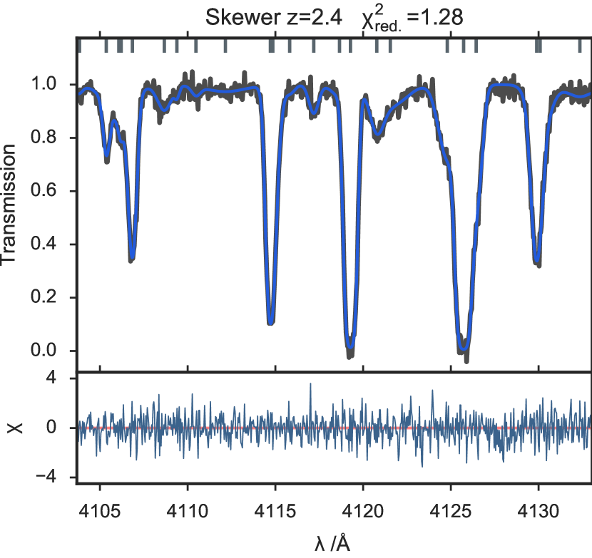
Figure 9.— A VP-fitted simulated line-of-sight at z=2.4. The blue line is the spectrum fitted by VPFIT. The underlying black line is the original skewer. Noise was generated based on our data to achieve a SNR of 52 per pixel at continuum level. The simulation used had a best fit temperature-density relation with $\gamma$=1.52, $\log T_{0}/\text{K}=4.07$ and a smoothing scale of $\lambda_{P}=70\,\text{kpc}$

. Underneath we we plot the resulting $\chi=(F_{\text{spec}}-F_{\text{fit}})/\sigma_{F_{\text{fit}}}$.

3.4. VP-fitting Simulations

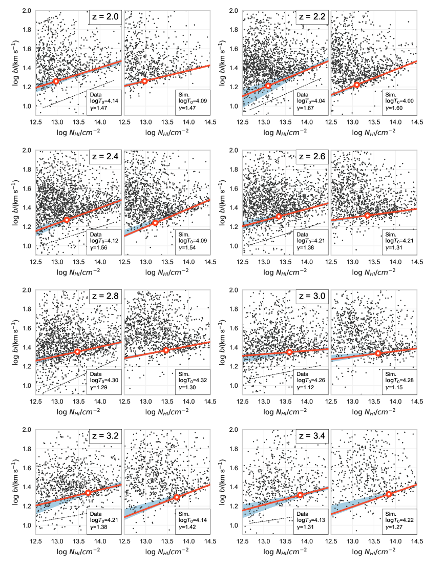
Figure 10.— Comparison of $b$-$N_{\text{HI}}$ distributions and cutoff fits for every redshift bin. At each redshift our data are shown in the left panel, while the simulated $b$-$N_{\text{HI}}$ distribution is shown in the right panel. The simulated $b$-$N_{\text{HI}}$ distributions shown are the ones that have $T_{0}$ and $\gamma$ closest to our final results (which will be introduced in § 5). The best cutoff fits (red) and 2$\sigma$-rejection (black dashed, data only) lines are overplotted. The shaded blue region represents the 68% confidence region of the fits to bootstrap realizations at every column density. The value of $N_{\text{HI,0}}(z)$ is plotted as an open red point (the choice of $N_{\text{HI,0}}$ is motivated in § 4.2). Noise and resolution effects were added to skewers based on the properties of our data. The cutoff fitting algorithm responds similarly to data and models once the contamination in the data is removed using the 2$\sigma$ rejection algorithm. The remaining contamination in the data is still more severe than in the models. This affects how the cutoff fitting procedure reacts to different bootstrap realizations.

We apply the exact same Voigt-profile fitting scheme described in § 2.2 to the forward modeled simulated skewers generated for different combinations of $T_{0}$, $\gamma$ and filtering scale $\lambda_{P}$. A Voigt-profile fit of a mock spectrum is shown in Figure 9. We then generate a $b$-$N_{\text{HI}}$ distribution for all our models and apply the same cutoff fitting algorithm described in § 2.3.3. We have checked for the effect of applying the $2\sigma$ rejection algorithm (as described in § 2.3.2) on the $b$-$N_{\text{HI}}$ distributions from simulated spectra and found that, given that there are a few outliers and no metal contamination, the effect is negligible. Therefore, we decided not to apply the $2\sigma$ rejection algorithm to simulated $b$-$N_{\text{HI}}$ distributions.

In Figure 10 we compare the $b$-$N_{\text{HI}}$ distributions and the respective cutoff fits of data (with metal lines excluded, see section 2.3.1) and mock spectra at all redshift bins. In both data and simulations, a cutoff in the distribution is evident. We also overplot the best fit cutoff (red) and the 68% confidence regions (light blue) determined by bootstrapped fits, as described in § 2.4. To illustrate the similarities of data and models, the model shown at each redshift is one that has $T_{0}$ and $\gamma$ closest to our final measurement presented in § 5.

The main difference is that the $b$-$N_{\text{HI}}$ distribution of the data exhibits more lines underneath the cutoff, i.e. in the low $b$ and low $N_{\text{HI}}$ part of the panels in Figure 10. As the SNR distribution is comparable in both diagrams, as well as the amount of blended absorption systems, we conclude that, if the model assumptions are right, these are most likely metal lines wrongly identified as Ly$\alpha$ absorption lines. Most of these narrow lines are excluded using the 2$\sigma$ rejection described in § 2.3.2, as indicated by the black dashed lines in the left panels of Figure 10. This leads to the conclusion that we are able to generate $b$-$N_{\text{HI}}$ distributions from our simulations that are similar to those retrieved from data in terms of the cutoff.

4. Calibration of the Cutoff Measurements

In this section we want to use our simulations to quantify how our cutoff observables $b_{0}$ and $\Gamma$ are related to the thermal parameters $T_{0}$ and $\gamma$. Once this calibration is known, it can be applied to our data and, under the assumption that simulated and measured $b$-$N_{\text{HI}}$ distributions are similar, we can retrieve $T_{0}$ and $\gamma$ from the data.

4.1. Formalism

To motivate this calibration we start with the temperature-density relation (Hui & Gnedin 1997; McQuinn & Upton Sanderbeck 2016), that states that the temperature distribution as a function of gas density is set by the temperature at mean density $T_{0}=T(\rho_{0})$ and the index $\gamma$:

$$\log T=\log T_{0}+(\gamma-1)\log(\rho/\rho_{0}$$ (4)

where $\gamma$ adjusts the contrast level of how much overdensities are hotter/cooler than underdensities.

In order to construct a relation between $b_{0}$ and $T_{0}$ as well as between $\Gamma$ and $\gamma$ we follow the Ansatz presented by Schaye (2001). It states that the overdensity $(\rho/\rho_{0})$ and the overdensity in terms of the column density $(N_{\text{HI}}/N_{\text{HI,0}})$, where $N_{\text{HI,0}}$ is the column density corresponding to the mean density $\rho_{0}$, are connected via a power law

$$\log(\rho/\rho_{0})=A+B\log(N_{\text{HI}}/N_{\text{HI,0}}).$$ (5)

Furthermore, for absorbers along the cutoff for which turbulent line broadening is negligible, the line broadening is purely thermal resulting in power law relation between $b_{\rm th}$ and $T$

$$\log T=C+D\log b_{\rm th},$$ (6)

where $b_{\rm th}$ is the thermal Doppler broadening. Combining eqns. (4.1),  (5) and (6) results in a power law relation between $b_{\rm th}$ and $N_{\rm HI}$ (eqn. (1)) which is the functional form that we fit to the cutoff of the $b$-$N_{\text{HI}}$ distribution. The coefficients in eqn. 1 can be written as:

$$\log b_{0}=\frac{1}{D}(\log T_{0}-C+A(\gamma-1))$$ (7)

$$(\Gamma-1)=\frac{B}{D}(\gamma-1).$$ (8)

Eqn (1) represents the line of minimal broadening at a given column density $N_{\text{\text{HI}}}$ (therefore $b_{\rm th}$), because absorbers in this relation are strictly thermally broadened. If the normalization constant $N_{\text{\text{HI}},0}$ is chosen so that it represents the column density value of a cloud with mean-density, then $A=0$ (see eqn. (5)), i.e. the dependency on $\gamma$ disappears from $\log b_{0}$ in eqn. (7). Taking this into account and redefining $\kappa=\frac{D}{B}$ we can re-write these equations as:

$$\log T_{0}=D\log b_{0}+C$$ (9)

$$(\gamma-1)=\kappa(\Gamma-1)$$ (10)

We can calibrate these relations by fitting the cutoff of mock datasets extracted from our simulations in combination with the same cutoff fitting algorithm we applied to the data. This approach has the advantage that it does not require the assumption that gas is only thermally broadened. Thus we can account for the effects of pressure smoothing and thermal broadening on the position of the cutoff in a generalized way.

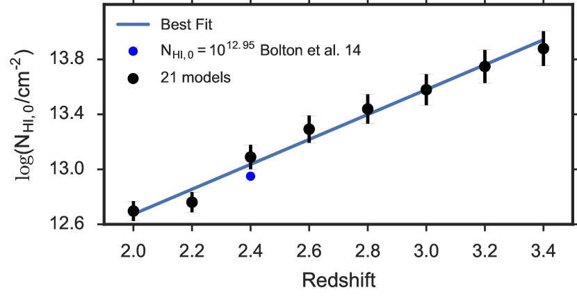
Figure 11.— Values of $N_{\text{HI,0}}$(z) from our simulations. The black points are calculated based on the mean flux correction from Becker et al. (2011) applied to our skewers using eqn (2). The error bars reflect the variance in the mean flux re-scaling value (i.e the strength of the UVB) and $T_{0}$ in the 26 models used in this work. The blue line is a linear fit to the black points, which will be used for estimating $N_{\text{HI,0}}$(z) in this work. For comparison, we show $N_{\text{HI,0}}(z=2.4)$ from Bolton et al. (2014), from hydrodynamic simulations.

4.2. Estimation of $N_{\text{HI,0}}$

The motivation for normalizing the $N_{\text{\text{HI}}}$ values with $N_{\text{\text{HI}},0}$, is that it simplifies the calibration between the $b$-$N_{\text{\text{HI}}}$ relation and the $T$-$\rho$ relation to be a one-to-one mapping between $b_{0}$-$T_{0}$ and $\gamma-\Gamma$ (equations (9) and (10)), with the former governed by two parameters $(C,D)$ and the latter governed by a single parameter $\kappa$. In other words, any $\gamma$ dependency is removed from eqn. (9).

However, in general the mapping between Ly$\alpha$ optical depth and density, and hence between $N_{\text{\text{HI}}}$ and density depends on the thermal parameters and the metagalactic photoionization rate $\Gamma_{\text{ion,HI}}$. This means that in principle $N_{\text{\text{HI}}}$ =$N_{\text{\text{HI}}}$$(\Gamma_{\text{ion,HI}},T_{0},\gamma)$, which can be seen directly from eqn. (2), as the temperature is a function of $T_{0}$ and $\gamma$. This would require determining $N_{\text{\text{HI}},0}$ for every single thermal model in order to calibrate the simple relations of eqns (9) and (10). Luckily, eqn. (2) illustrates that the thermal parameter dependency is quite weak scaling as $T^{-0.22}$. Instead, the primary dependency is on $\Gamma_{\text{ion,HI}}$. Furthermore, because one always adjusts the mean UVB to give the same mean flux for different thermal models, the variation of $N_{\text{\text{HI}}}$ with thermal parameters is even further reduced.

The approach that was used in Rudie et al. (2012a) to compute $N_{\text{\text{HI}},0}$ was to adopt a fixed value of $\Gamma_{\text{ion,HI}}$ and compute $N_{\text{HI}}$ analytically, i.e. $N_{\text{\text{HI}},0}$ = $N_{\text{\text{HI}}}$$(\Delta=1)$. Bolton et al. (2014) instead adopted the average value of $N_{\text{\text{HI}}}$ associated with gas at mean density in his simulations. In this work we compute $N_{\text{\text{HI}},0}$ analytically using eqn (2) evaluated at mean-density, i.e. $\Delta=1$, for the parameters $\Gamma_{\text{ion,HI}}$ and $T_{0}$ from our simulations. Note that we use the effective UV background $\Gamma_{\text{ion,HI}}=\Gamma_{\text{ion,HI,sim}}/A_{r}$, because our simulations were re-scaled to give the correct mean flux at a given redshift (see section 3.1). Figure 11 shows the average and 1$\sigma$ range of our $N_{\text{\text{HI}},0}$ values over all of our thermal models as a function of redshift. This confirms that the variation of $N_{\text{\text{HI}},0}$ over the different thermal models is small, as also argued by Bolton et al. (2014).

Finally, we applied a fit to the mean values of $N_{\text{HI,0}}$ over the 26 different simulations taking the standard deviation as an estimate for the error. The best fit linear function has the form

$$\log({N_{\text{HI,0}}/\text{cm}^{-2}})(z)=a(1+z)+c$$ (11)

with $a=0.6225$ and $c=11.1068$. Throughout this work we will use this function to compute $N_{\text{HI,0}}$ values at fixed redshifts.

Our best fit value of $N_{\text{\text{HI}},0}$ at $z=2.4$ $N_{\text{HI,0}}\simeq 10^{13.22}$ cm^-2 is inconsistent with the value measured by Bolton et al. (2014) $N_{\text{HI,0}}=10^{12.95}$ cm^-2, presumably because of the high values of $\Gamma_{\text{ion,HI}}$ they needed to match the opacity measurements by Becker & Bolton (2013). Part of this possible discrepancy could be due to the lower temperature in Bolton et al. (2014), but the dependency of $N_{\text{\text{HI}}}$ on $T_{0}$ is too small to drive this difference. While Bolton et al. (2014) simulations require a value of $\Gamma_{\text{ion,HI}}/10^{-12}\text{s}^{-1}=1.86$ to match $N_{\text{\text{HI}}}$ to optical depth weighted density using Schaye’s relation (eqn. 2), we use the re-scaled values of our simulations, which are consistent with Becker & Bolton (2013) to directly calculate $N_{\text{\text{HI}},0}$. This difference of $\sim 0.3$ dex will certainly lead to inconsistent values of $b_{0}$, but since the calibration process is carried out using the same values of $N_{\text{\text{HI}},0}$ for both the data and simulations, the calibration will cancel out differences due to $N_{\text{\text{HI}},0}$ when dealing with $T_{0}$ as long as the scatter due to $\gamma$ dependency in eqn. 9 remains small compared to our statistical error in $b_{0}$. We further discuss this in § 5.3 when we compare our final measurements to Bolton et al. (2014).

4.3. Calibration Using Simulations

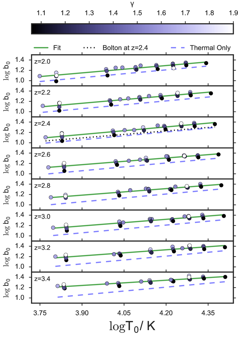
Figure 12.— Calibration of the $\log b_{0}$ vs. $\log T_{0}$ relation. Each point corresponds to a simulated $b$-$N_{\text{HI}}$ distribution. The points are colored based on their $\gamma$ value. The green line is the best two parameter fits to the points. The blue-dashed line represents the case when the value of $b_{0}$ is due to pure thermal broadening. The scatter is due to unmodelled $\lambda_{P}$ effects as well as deviations due to $\gamma$-dependency of this relation when $N_{\text{HI,0}}$ does not exactly correspond to the mean-density. At redshift $z=2.4$ we show the line corresponding to the calibration carried out by Bolton et al. (2014) using hydrodynamic simulations (black dashed).

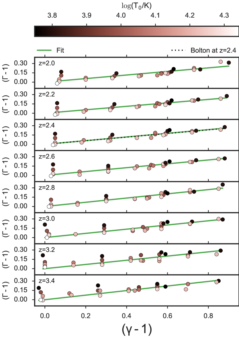
Figure 13.— Calibration of the $(\Gamma-1)$ vs. $(\gamma-1)$ relation. Each point corresponds to a simulated $b$-$N_{\text{HI}}$ distribution. The points are colored based on their $T_{0}$ value. The green line represents the best one parameter fits to the points. This calibration seem to be independent of the corresponding $T_{0}$ and $\lambda_{P}$ values. At redshift $z=2.4$ we show the line corresponding to the calibration carried out by Bolton et al. (2014) using hydrodynamic simulations (black dashed).

In order to generate the calibration between $b_{0}$-$T_{0}$ and $\Gamma$-$\gamma$ we ran our cutoff fitting algorithm on simulated $b$-$N_{\text{HI}}$ distributions, each constructed from 100 mock spectra drawn from all of our 26 thermal models at each redshift. The results are shown in Figures 12 and 13, respectively. There we see the simulation input values of $T_{0}$ and $(\gamma-1)$ for our 26 thermal models plotted against the values of $b_{0}$ and $(\Gamma-1)$ extracted from cutoff fits to each $b$-$N_{\text{HI}}$ distribution. Each panel corresponds to a different redshift which allows us to capture the evolution of the calibration. The green lines are the fits using eqns. (9) and (10) at every redshift. For comparison, we show the calibration of Bolton et al. (2014) at $z=2.4$ in black. In the $\log T_{0}$-$\log b_{0}$ diagrams we additionally plot the case in which $b_{0}$ arises purely due to thermal broadening, i.e. $b_{0}=\sqrt{2k_{B}T_{0}/m_{\text{HI}}}$.

The points shown in the diagrams are the median values of $b_{0}$ and $\Gamma$ from 500 random realizations of the $b$-$N_{\text{HI}}$ distributions with replacement rather than the best-fit value of the cutoff parameters of the mock $b$-$N_{\text{HI}}$ distribution. We chose this approach for consistency with how we treated the data, but the results are essentially insensitive to this choice.

Our $26$ models have different contributions to the thermal broadening $b_{0}$ due to the different values of the pressure smoothing scale $\lambda_{P}$. Similarly, the fact that we assumed one value of $N_{\text{HI},0}$ for all models with same redshift will introduce a small $\gamma$ dependency in the $\log T_{0}$-$\log b_{0}$ relation. We want to include our lack of knowledge about $\lambda_{P}$ and additional effects in the calibration by quantifying the amount of scatter that they add into the calibration relations. This is done by simultaneously fitting equations (9) and (10) to the same 2000 bootstrap realizations of the points in the $\log T_{0}$-$\log b_{0}$ and $(\gamma-1)$-$(\Gamma-1)$ diagrams with replacement. The best fit values for every bootstrap realization are stored, giving us the approximated pdfs $p(D,C)$ and $p(\kappa)$.

For illustration, the calibration values as a function of redshift are shown in Figure 14. The error bars correspond to the 68% confidence intervals of $p(\kappa)$ and the marginal distributions of $p(D,C)$. The errors in $\kappa$ are small because the scatter in the $(\gamma-1)$-$(\Gamma-1)$ relation is only slightly driven by dependencies on $T_{0}$ or $\lambda_{P}$.

While we agree with the measurements of $C,D$ from Bolton et al. (2014) at $z=2.4$ in terms of the marginalized distributions of $C,D$, his calibration values are about 2$\sigma$ off in terms of the joint PDF $p(C,D)$ as shown in Figure 15. This could be attributed to the difference in method used for cutoff fitting (Bolton et al. 2014 uses least absolute deviation while we use a least-squares minimization approach for the cutoff fitting) as well as the difference in $N_{\text{\text{HI}},0}$. The calibration constant $\kappa$ between $(\gamma-1)$ and $(\Gamma-1)$ we derived agrees within 1$\sigma$ with the value reported by Bolton et al. (2014).

The impact of the calibration differences is further discussed when we compare our $T_{0}$ and $\gamma$ results to previous works in § 5.3.

5. Results

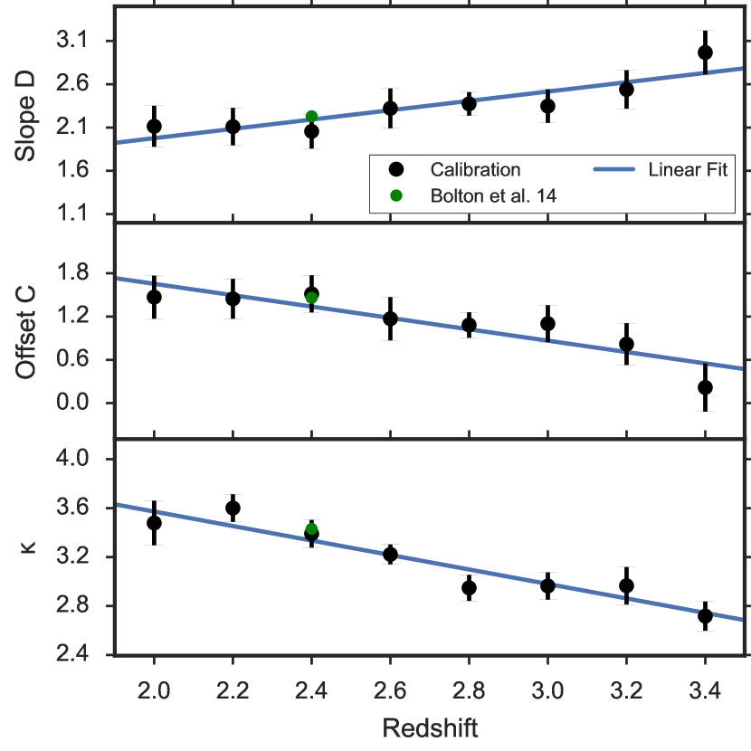
Figure 14.— Upper panels: Bootstrapped fit values to the $\log b_{0}$ vs. $\log T_{0}$ relation. The error bars reflect the 68% confidence levels of the marginal distributions of the bootstrapped $p(D,C)$ pdf at each redshift. Lower panel Bootstrapped fit values to the ($\Gamma-1$) vs. ($\gamma-1$) relation. The error bars reflect the 68% confidence levels of the bootstrapped $p(\kappa)$ pdf at each redshift. The blue lines are linear fits to guide the eye.

5.1. Evolution of $T_{0}$ and $\gamma$

Concerning the evolution of $\gamma$, the first conclusion we can draw directly from the data cutoff measurements shown in Figure 6 is that a positive ($\Gamma-1$) is preferred for all redshift bins. This implies, see eqn (10), that a positive temperature-density relation index ($\gamma-1$) is favored at all redshifts probed. In the $p(b_{0},\Gamma)$($z=3$) panel in Figure 7 about 4% of the points in $p(b_{0},\Gamma)$ are consistent with $\Gamma<1$.

Having both the cutoff measurements and the calibration in hand, we can now estimate $T_{0}$ and $\gamma$. It is clear from Figure 7 that covariance in the cutoff fits will lead to a similar covariance between $T_{0}$ and $\gamma$, and furthermore, that the scatter in our calibration quantified in Figure 14 has to be incorporated into the error budget. To include all of these effects and arrive at the joint probability distribution $p(T_{0},\gamma)$ we adopt a Monte Carlo approach as follows. We combine 2000 bootstrapped $b_{0}$ and $\Gamma$ pairs in $p(b_{0},\Gamma)$ with every single of the 2000 points in the bootstrapped calibration pdfs $p(D,C)$ and $p(\kappa)$ from simulations using eqns. (9) and (10) at every redshift bin. The contours of the 2000$\times$2000 points in $p(T_{0},\gamma)(z)$ estimated via kernel density estimation at every redshift are shown in Figure 16. Comparison with Figure 7 indicates that the shape of the $T_{0}$-$\gamma$ contours are qualitatively similar to the $b_{0}$-$\Gamma$ contours, which results from noise and degeneracy in fitting the cutoff. This is expected from eqns. 9 and 10. The contours are slightly broadened by the calibration uncertainty. Note that uncertainties in $T_{0}$ and $\gamma$ are dominated by the statistical errors of $b_{0}$ and $\Gamma$ due to the high precision of the calibration process.

The evolution of the temperature at mean density $T_{0}$ and index of the temperature-density relation $\gamma$ measured in this work is shown in Figures 17 and 18. The error bars are calculated using the 16 and 84 percentiles of the marginal distributions of $T_{0}$ and $\gamma$ from $p(T_{0},\gamma)$. The main features are that the temperature at mean-density increases from $z=3.4$ to $z=2.8$ (peaking at $T_{0}\simeq 20000$ K), while $\gamma$ has its lowest value $\gamma=1.12$ at $z=3.0$. From $z=2.8$ to $z=2.0$, $T_{0}$ decreases again towards $T_{0}\simeq 10000$ K while $\gamma$ increases gradually towards $\gamma\simeq 1.6$.

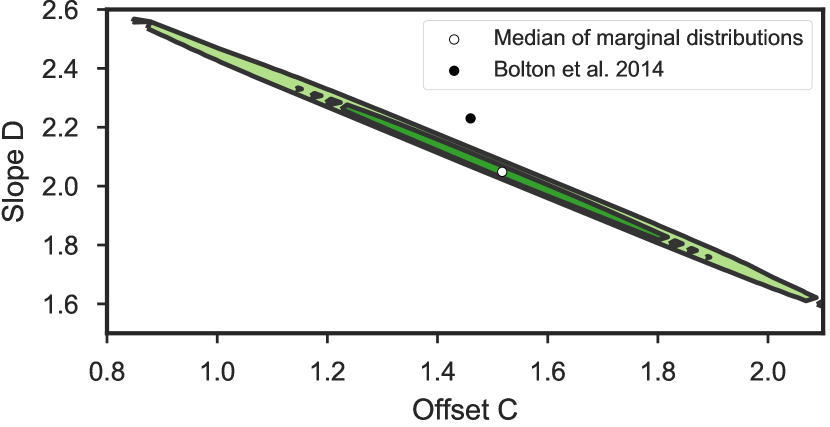
Figure 15.— Comparison of the $b_{0}$-$T_{0}$ calibration values with Bolton et al. (2014) at $z=2.4$ in terms of the joint distribution of $C,D$. The 68% confidence levels are plotted in dark green and 95% in light green.

We tested if the evolution of $T_{0}$/$\gamma$ is consistent with a peak/dip by comparing $\chi^{2}$-distributions $P(\chi^{2}|{\rm dof})$ of fits to our measurements, where dof is the number of degrees of freedom. For this purpose we use a 4-parameter piecewise linear function $f(z)$ of the form

$$f(z)=\begin{cases}s_{1}(z-z_{\rm br})+o&z<z_{\rm br}\\ s_{2}(z-z_{\rm br})+o&z\geq z_{\rm br},\end{cases}$$ (12)

shown in light gray in Figure 17, that describes two linear function parametrized with two slopes $s_{1}$ and $s_{2}$, an offset $o$ and a break redshift $z_{\rm br}$. For comparison we also compute the best fits for a 2-parameter linear evolution and a constant. For the evolution of $T_{0}$, a piecewise linear function with a best fit break at $z_{\rm br}=2.9$ results in a $P(\chi^{2}|{\rm dof})=0.097$ for 4 dof. The best fit linear evolution results in $P(\chi^{2}|{\rm dof})=6.5\times 10^{-4}$ for 6 dof, while no evolution in $T_{0}$ results in $P(\chi^{2}|{\rm dof})=2.4\times 10^{-4}$ for 7 dof. This provides some indication that our measurements prefer a model with a peak in the temperature. In the case of $\gamma$, a piecewise linear function with a break at $z_{\rm br}=3.0$ results in a $P(\chi^{2}|{\rm dof})=0.12$. This is only slightly better than $P(\chi^{2}|{\rm dof})=0.06$ that we observe for the linear evolution model and best fit constant $\gamma=1.4$ with $P(\chi^{2}|{\rm dof})=0.01$. This suggests that a dip in the evolution of $\gamma$ is slightly preferred given the size of our error bars. A comparison of all fits including the reduced $\chi^{2}$ is given in Table 3.

The peak in $T_{0}$ is suggestive of a late time $z\sim 3$ process heating the IGM. The reionization of singly ionized helium He II (He II $\rightarrow$ He III) by a QSO driven metagalactic ionizing background is the most obvious candidate that would produce such an effect. It has also been argued that HeII reionization ends around $z\sim 3$ (Worseck et al. 2011), which coincides with the redshift at which our measurements of $T_{0}$ appear to peak (Upton Sanderbeck et al. 2016; Puchwein et al. 2015; Oñorbe et al. 2017).

Additionally, if the temperature increase comes about independently of the density of the IGM, i.e. the photoionization rate is much higher than the recombination rate everywhere, then the IGM is driven to a temperature-density relation that is close to isothermal (see non-equilibrium simulations in Puchwein et al. 2015). This causes a flattening of the temperature-density relation, which corresponds to a dip in the evolution of $\gamma$. In case that the amount of heating is proportional to the neutral fraction of the gas, e.g. high density regions with higher recombination rate experience more heating, then the flattening of $\gamma$ is expected to be less prominent (Puchwein et al. 2015). Given that our data only slightly prefers a dip in $\gamma$ over a constant evolution, we can not clearly disentangle these scenarios. Furthermore, the evolution of $\gamma$ seems to be consistent with a constant if we apply a least absolute deviation method for the cutoff fitting (see Appendix B).

Table 3Goodness of fit for different models.

Function	Param.	dof	$P(\chi^{2}|{\rm dof})$	$\chi^{2}_{\text{red.}}$
Constant	$T_{0}$	7	$2.4\times 10^{-4}$	3.67
	$\gamma$	7	0.01	2.13
Linear	$T_{0}$	6	$6.5\times 10^{-4}$	3.56
	$\gamma$	6	0.06	1.42
Piecewise Linear	$T_{0}$	4	0.097	1.30
	$\gamma$	4	0.12	1.11

After HeII reionization and its concomitant heat injection are complete, the IGM is expected to cool down on a timescale of several hundred Myr (Hui & Gnedin 1997; McQuinn & Upton Sanderbeck 2016), or $\Delta z\sim 1.0$, and asymptote to a $T_{0}$ and $\gamma$ set by the interplay of the photoionization heating and adiabatic cooling, independent of the details of reionization. Due to this process, the IGM is heated by photoionization and then left to cool by cosmic expansion once most of the He II is ionized. This physical picture is consistent with our measured evolution of $T_{0}$ and $\gamma$.

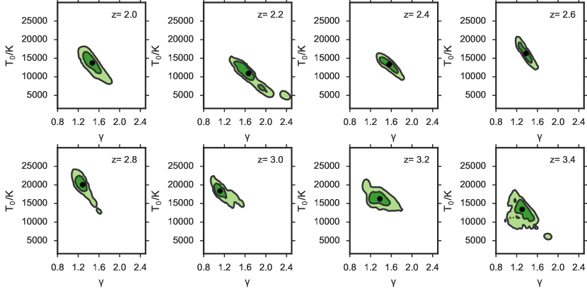
Figure 16.— Resulting $p(T_{0},\gamma)$ pdfs. This is the combination of our data-measured $p(b_{0},\Gamma)$ pdfs with the simulation-extracted calibration $p(\kappa)$ and $p(A,B)$ pdfs. Each panel represents a redshift bin of size $\delta z=0.2$. The 68% confidence levels are plotted in dark green and 95% in light green. The black point corresponds to the median of the marginal distributions of $T_{0}$ and $\gamma$.

5.2. Comparison with Models

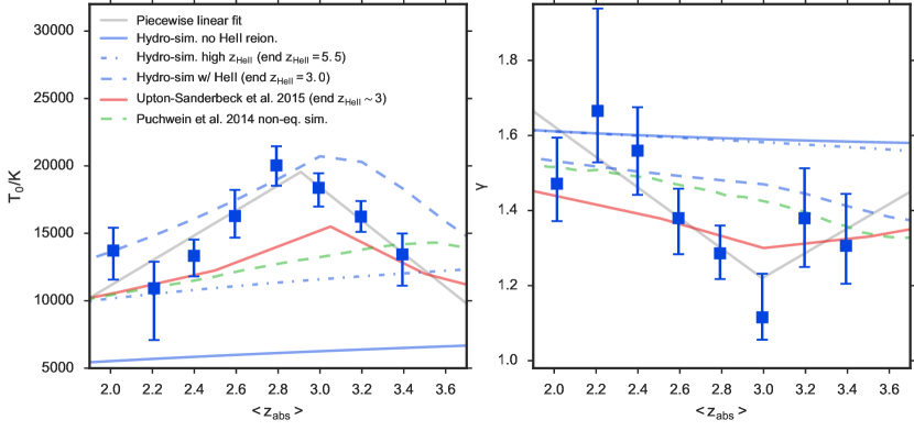
Figure 17.— Evolution of $\gamma(z)$ and $T_{0}(z)$ compared to models. The measurements come from the marginal distributions of $p(T_{0},\gamma)$ generated by combining all points in the bootstrapped pdf $p(b_{0},\Gamma)$ from the data cutoff fits with all points in the calibration pdfs $p(C,D)$ and $p(\kappa)$ using eqns. 9 and 10. The error bars are estimated using the 16 and 84 percentiles of the marginal distributions of $p(T_{0},\gamma)$. For comparison we plot 3 different Nyx simulations from Oñorbe et al. (2017), a semi-analytical models by Upton Sanderbeck et al. (2016) and a non-equilibrium reionization simulation by Puchwein et al. (2015). A best fit 4-parameter piecewise linear function (described in § 5.1) is shown in light gray.

In Figure 17, we compare our measurements to a semi-analytical model by Upton Sanderbeck et al. (2016) constructed by following the photoheating history of primordial gas (red solid line) and non-equilibrium reionization simulations by Puchwein et al. (2015). We also compare to different thermal histories from the THERMAL suite (blue curves from Nyx simulations, Almgren et al. 2013; Lukić et al. 2015). Each Nyx simulation was run using different UVB and applying different heat inputs to create three different thermal histories following the method introduced in Oñorbe et al. (2017): (1) No He II reionization (blue solid line) (2) He II reionization ending at z =3 with a temperature input $\Delta T_{\text{HeII}}=3\times 10^{4}$K (blue dashed line) and (3) He II reionization ending at $z=5.5$ with a temperature input $\Delta T_{\text{HeII}}=1.5\times 10^{4}$K (blue dot-dashed line).

First we note that if He II reionization never happened or ended at high redshift, then the simulations suggest that $T_{0}$ would be $\sim 10000$K lower than our measurements at $z=3$. Furthermore, in agreement with the models, the temperature at mean density decreases at $z<3$. Our measurements suggest that $T_{0}$ is higher than the Upton Sanderbeck et al. (2016) fiducial model and Puchwein et al. (2015) non-equilibrium simulation, with the difference that the non-equilibrium simulation peaks at higher redshift.

The evolution of $\gamma$ from Upton Sanderbeck et al. (2016) shows a dip at $z=3$ nearly at the same position as our lowest measurement. The $\gamma$ dip in the non-equilibrium simulation appears at higher redshifts, coinciding with the corresponding peak in $T_{0}$. The thermal evolution of the Nyx simulation (2), with He II reionization at $z=3$, shows a larger $\gamma$ at this redshift because the heating due to He II reionization in the model is more extended and already started at higher redshift (see Oñorbe et al. 2017 for more details on the models and their intrinsic limitations). In summary, our measurements of $T_{0}$ are suggestive of a heating event taking place between $z=3.4$ and $z=3$.

5.3. Comparison with Previous Work

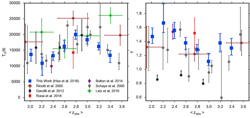
Figure 18.— Evolution of $\gamma(z)$ and $T_{0}(z)$, based on the marginal distributions of the $p(T_{0},\gamma)$ pdfs, compared to previous measurements.

We can directly compare our cutoff fitting results at $z=2.4$ with those presented in Rudie et al. (2012a), shown in the $z=2.4$ panel of Figure 6. At $z=2.4$, our bootstrapped cutoff position measurement yields $\Gamma=1.17\pm 0.03$, which is in good agreement with $\Gamma=1.156\pm 0.032$ measured by Rudie et al. (2012a). If we evaluate their measurement $b_{0R}=b(N_{\text{HI,0}}=10^{13.6}\leavevmode\nobreak\$cm^-2$)=17.56\pm 0.4$ km/s at the position of our $N_{\text{HI,0}}(z=2.4)=10^{13.22}$ cm^-2 while keeping their $\Gamma$ fixed, this measurement becomes $b_{0R}^{\prime}=15.32\pm 0.55$ km/s. Our measurement $p(b_{0},\Gamma)$ marginalized over $\Gamma$ (with $b_{0}=18.68^{+0.74}_{-1.07}$ km/s) is more than $3\sigma$ higher than this value, indicating tension between our measurements and Rudie et al. (2012a) in terms of $b_{0}$. This discrepancy is probably due to a different implementation of the cutoff and VP-fitting algorithms used. We performed a cutoff fit our data at $z=2.4$ using a least absolute deviation algorithm and although it tends to lead to smaller values of $b_{0}$, we can not reproduce this low cutoff.

The left panel of Figure 18 shows a comparison of our $T_{0}$ evolution with previous measurements. Our measurements of $T_{0}$ are in good agreement with those of Schaye et al. (2000). We disagree with Ricotti et al. (2000) at $z>2.4$, where we tend to measure significantly lower temperatures.

Note that our $T_{0}$ measurement agrees with Bolton et al. (2014), who recalibrated the cutoff measurement of Rudie et al. (2012a) at $z=2.4$. The fact that we measure inconsistent values of $b_{0}$ should lead to inconsistent values in $T_{0}$. However, given the difference in our calibration values $D,\leavevmode\nobreak\ C$, this inconsistency is alleviated. Furthermore, Bolton et al. (2014) added a systematic error contribution to his statistical uncertainty in $T_{0}$ due to scatter in the $N_{\rm HI}$-overdensity relation in his simulations, that lead to a 0.2 dex uncertainty in $N_{\text{\text{HI}},0}$. When adopting values of $N_{\text{\text{HI}},0}$ that are 0.2 dex above/below the values determined in § 4.2 self consistently in our simulations and data, we observe that the calibration compensates for the choice of $N_{\text{\text{HI}},0}$, leading to negligible changes in the final results. In other words, choosing a higher value of $N_{\text{\text{HI}},0}$ will increase the value of $b_{0}$ almost equally in the data and simulations. Note that this is only true as long as the $\gamma$-dependency in eqn. 9 remains small. Since our uncertainty in $T_{0}$ is dominated by the statistical error of $b_{0}$, we adopt no systematic uncertainty term for $N_{\text{\text{HI}},0}$.

Our measurements are in good agreement with the wavelet amplitude PDF measurements by Garzilli et al. (2012). Comparison with wavelet decomposition measurements by Lidz et al. (2010) in our redshift range shows agreement at intermediate redshifts, but $>2\sigma$ disagreement at $z\sim 2.2$ and $3.4$. An analogous disagreement has been observed previously in Becker et al. 2011 (in the context of curvature measurements), but its source remains unclear.

We show a comparison of our $\gamma$ values with other measurements in the literature in the right panel of Figure 18. Our measurements of $\gamma$ agree with Schaye et al. (2000) and Ricotti et al. (2000). We also observe a low values of $\gamma$ at redshifts around $z=3$.

Our measurement of $\gamma$ at $z\simeq 2.4$ agrees with Bolton et al. (2014). This was expected given the agreement with Rudie et al. (2012a) in terms of $\Gamma$.

We present a detailed comparison of our measurements of $p(T_{0},\gamma)$ at $z=2.8$ with those of Rorai et al. (2018) in appendix B.

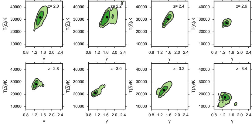
Figure 19.— Resulting $p(T(\bar{\Delta}),\gamma)$ pdfs. This is the combination of our calibrated $p(T_{0},\gamma)$ pdfs at every redshift with the measurements of $\bar{\Delta}$ by Becker et al. (2011). The 68% confidence levels are plotted in dark green and 95% in light green. The black point corresponds to the median of the marginal distributions of $T(\bar{\Delta})$ and $\gamma$.

5.4. Evolution of the Temperature at Optimal Density

The temperature-density relation is traditionally normalized at mean-density. However, at different redshifts an optical depth of $\sim 1$ in the Ly$\alpha$ forest traces different overdensities. Based on this, Becker et al. (2011) introduced the mean curvature statistic $\left<\left|\varkappa\right|\right>$, which is a probe of the thermal state of the IGM that is related to the temperature at optimal density $T(\bar{\Delta})=T(\rho_{\text{opt}}/\rho_{0})$ independently of $\gamma$.

For a fair comparison of our measurements with those from Becker et al. (2011), we apply another transformation on our measurements so we can look at the evolution of the temperature of the IGM in terms of the temperature at the optimal density $T(\bar{\Delta})$. If we re-write the temperature-density relation in terms of $T(\bar{\Delta})$:

$$T(\bar{\Delta})=T_{0}\bar{\Delta}^{\gamma-1}$$ (13)

we are able to combine our $p(T_{0},\gamma)$ pdf with measurements of $\bar{\Delta}$ by Becker et al. (2011), which have no reported uncertainties. Plugging in all pairs of $(T_{0},\gamma)$ from $p(T_{0},\gamma)$ into eqn. 13 in combination with a fixed value of $\bar{\Delta}$ (linearly interpolated based on Becker et al. 2011 to match our redshift bins) allows us to generate $p(T(\bar{\Delta}),\gamma)$ pdfs for each redshift. This approach takes into account any covariance with respect to $\gamma$ in our measurements. The resulting $p(T(\bar{\Delta}),\gamma)$ contours are shown in Figure 19. We note that covariance between $T(\bar{\Delta})$ and $\gamma$ is diminished compared to that between $T_{0}$ and $\gamma$ (see Figure 16 for comparison) when taking our measurements to $T(\bar{\Delta})$ space. However, note that our $T(\bar{\Delta})$ contours are correlated with $\gamma$ in most redshift bins.

Given $p(T(\bar{\Delta}),\gamma)$ joint distributions, we can marginalize out $\gamma$ and compare $T(\bar{\Delta}$) directly to Becker et al. 2011 and Boera et al. 2014 (also computed using the mean curvature method). Our 68% confidence regions for $T(\bar{\Delta})$ as a function of redshift are shown in Figure 20. A comparison with Becker et al. (2011) is not completely straightforward, given that the redshift bin sizes are different and we are also linearly interpolating their $\bar{\Delta}$ values. Broadly speaking, we see agreement with Becker et al. (2011) and Boera et al. (2014) at $1\sigma$ level at $z<2.4$, $z=3.0$ and $3.4$, as well as generally higher temperatures at $2.4\leq z\leq 3.2$ which disagree at the $>2\sigma$ level. Given the method dependency (see Appendix B) and other systematics associated with cutoff fitting, the difference might not be as significant as it appears, once these effects are properly quantified. Additionally, if one included uncertainties in $\bar{\Delta}$, it would further alleviate this tension. One possible effect that could be playing a role is that the curvature statistic is sensitive to metals in the Ly$\alpha$ forest that do not get masked, i.e. metal contamination leads to lower values of $T(\bar{\Delta})$ (Boera et al. 2014). This effect is potentially more prominent at higher redshifts where blending of Ly$\alpha$ forest lines makes it more difficult to identify all metals. Our analysis is in principle less sensitive to metals given our 2$\sigma$ rejection procedure adopted before cutoff fitting, but the exact source of this discrepancy remains unclear.

An overview of all quantities measured and adopted in this work is given in Table 4. A subset of the measurements on which the distributions $p(b_{0},\Gamma)$, $p(D,C)$, $p(\kappa)$ and $p(T_{0},\gamma)$ are based is available in machine-readable form for all redshifts presented and can be obtained in the Zenodo repository Hiss et al. (2018).

Table 4Measurements and values adopted

$z$	$b_{0}$	$D$	$C$	$T_{0}$	$\Gamma$	$\kappa$	$\gamma$	$\bar{\Delta}$	$T(\bar{\Delta})$
	(km/s)			(K)					(K)
2.0	$18.22^{+0.97}_{-1.39}$	$2.11\pm{0.245}$	$1.48\pm{0.305}$	$13721^{+1694}_{-2152}$	$1.14^{+0.03}_{-0.03}$	$3.48\pm{0.185}$	$1.47^{+0.12}_{-0.1}$	5.85	$31659^{+3690}_{-3455}$
2.2	$16.89^{+1.37}_{-3.12}$	$2.1\pm{0.225}$	$1.46\pm{0.285}$	$10927^{+1961}_{-3843}$	$1.19^{+0.07}_{-0.04}$	$3.6\pm{0.1}$	$1.67^{+0.27}_{-0.14}$	5.1	$31853^{+3415}_{-3126}$
2.4	$18.68^{+0.74}_{-1.07}$	$2.04\pm{0.19}$	$1.54\pm{0.25}$	$13334^{+1206}_{-1530}$	$1.17^{+0.03}_{-0.03}$	$3.39\pm{0.11}$	$1.56^{+0.12}_{-0.12}$	4.4	$30335^{+2976}_{-2617}$
2.6	$20.41^{+1.02}_{-0.87}$	$2.31\pm{0.23}$	$1.19\pm{0.3}$	$16281^{+1940}_{-1601}$	$1.12^{+0.02}_{-0.03}$	$3.22\pm{0.08}$	$1.38^{+0.08}_{-0.1}$	3.87	$27113^{+1234}_{-1372}$
2.8	$22.67^{+0.55}_{-0.6}$	$2.38\pm{0.135}$	$1.08\pm{0.175}$	$20036^{+1416}_{-1507}$	$1.1^{+0.02}_{-0.02}$	$2.95\pm{0.1}$	$1.29^{+0.07}_{-0.07}$	3.35	$28245^{+1729}_{-1750}$
3.0	$22.24^{+0.33}_{-0.73}$	$2.35\pm{0.19}$	$1.1\pm{0.25}$	$18371^{+1087}_{-1388}$	$1.04^{+0.04}_{-0.02}$	$2.96\pm{0.11}$	$1.12^{+0.12}_{-0.06}$	2.95	$21002^{+1171}_{-1596}$
3.2	$21.65^{+0.4}_{-0.52}$	$2.53\pm{0.23}$	$0.84\pm{0.3}$	$16244^{+1153}_{-1135}$	$1.13^{+0.04}_{-0.04}$	$2.96\pm{0.145}$	$1.38^{+0.13}_{-0.13}$	2.57	$23410^{+2623}_{-2409}$
3.4	$20.8^{+0.71}_{-1.27}$	$2.97\pm{0.265}$	$0.22\pm{0.35}$	$13439^{+1542}_{-2318}$	$1.11^{+0.05}_{-0.04}$	$2.72\pm{0.12}$	$1.31^{+0.14}_{-0.1}$	2.3	$17500^{+2289}_{-1542}$

Note. — Summary of all quantities measured/used in this work. The first column shows the center of each redshift bin used. The second column shows the median and percentile based errors of the cut-off fitting parameter $b_{0}$. The third and fourth columns show the calibration parameters $C,D$ from eqn (9). The fifth column shows the resulting $T_{0}$ once the calibration is applied. The sixth column shows the median and percentile based errors of the cut-off fitting parameter $\Gamma$. The seventh column shows the calibration parameter $\kappa$ from eqn (10). The eigth column shows the resulting $\gamma$ once the calibration is applied. The ninth column shows the values of the optimal-density that were linearly interpolated from Becker et al. (2011). The last column shows the values of the temperature at optimal density $T(\bar{\Delta})$ constructed using eqn. (13).

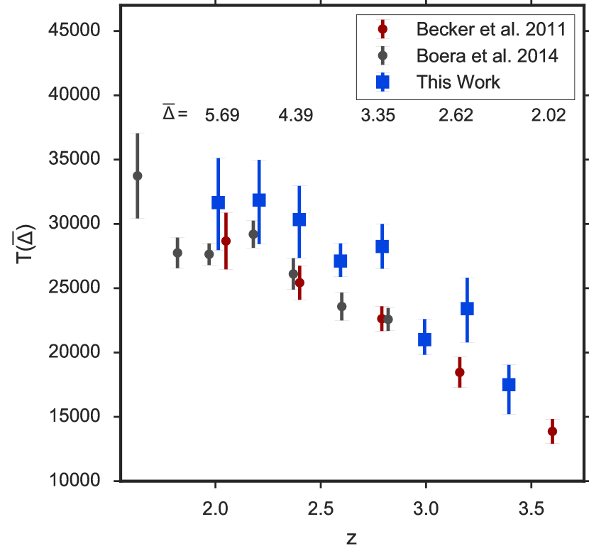
Figure 20.— Comparison to Becker et al. (2011) and Boera et al. (2014) after combining our $p(T_{0},\gamma)$ with Becker et al. (2011) measurements of $\bar{\Delta}$. We measure a hotter IGM at higher redshifts.

5.5. Caveats

It should be noted that there are a number of assumptions adopted in our work that we summarize as follows.

We assume that the simulated $b$-$N_{\text{HI}}$ distributions are comparable to the ones extracted from the data, or in other words, that the cutoff fitting algorithm will respond similarly in both cases. This is a specially problematic assumption, because metals have to be rejected from our data which are by construction not present in the simulated mock spectra. Therefore, we observe that the $b$-$N_{\text{HI}}$ distributions from mock spectra generate much more concentrated cutoff fitting bootstraps (see Figure 10). This effect increases the errors measured in $b_{0}$ and $\Gamma$ in the data, which dominate the error budget of $T_{0}$ and $\gamma$. Furthermore, our simulations do not account for effects such as multimodality in the temperature-density relation which could play a role specially at $z>2.8$.

Another assumption is that the calibrations for $T_{0}$ and $\gamma$ can be done separately, i.e. $p(D,C,\kappa)=p(D,C)p(\kappa)$. This is not necessarily true, as these parameters could be correlated. As we calculated the calibration values on the same bootstrap samples, any correlation is still preserved. We inspected the distributions of $p(\kappa,C)$ and $p(\kappa,D)$ and did not find significant correlation.

In this work we utilize a least-square fitting algorithm in every iteration of the cutoff fitting process. This is a different approach than in previous works and our final results are sensitive to the method chosen. This aspect is further discussed in the appendix B in the context of the comparison of our work with the results of Rorai et al. (2018).

As mentioned in Schaye et al. (1999), if the reionization process has large spatial fluctuations and the gas has not settled into one temperature-density relation (Compostella et al. 2013; McQuinn & Upton Sanderbeck 2016, see), the measurement of the position of the cutoff will be sensitive to the gas with the lowest temperature. If this is the case, the temperature measurements should be treated as lower limits to the average temperature.

6. Summary

In this work we assessed the thermal state of the IGM and its evolution in the redshift range $2.0<z<3.4$ using 75 high SNR and high resolution Ly$\alpha$ forest spectra from the UVES and HIRES spectrographs. We exploit the fact that absorbers that are primarily broadened due to the thermal state of the gas have the smallest Doppler parameters, which results in a low-$b$ cutoff in the $b$-$N_{\text{HI}}$ distribution. We decomposed the Ly$\alpha$ forest of these spectra into a collection of Voigt profiles, and measured the position of this cutoff as a function of redshift. We calibrate this procedure using 26 combinations of thermal parameters at each redshift from the THERMAL suite of hydrodynamic simulations, with different values of the IGM pressure smoothing scale. We conduct an end-to-end analysis whereby both data and simulations are treated in a self-consistent way, and uncertainties in both the cutoff fitting, and the calibration procedure are propagated into our analysis.

The primary results of this work are:

• We see suggestive evidence for a peak in IGM temperature evolution at $z\simeq 2.9$. The temperature at mean density $T_{0}$ increases with decreasing redshift over the range $2.9<z<3.4$, peaks around $z\simeq 2.9$, and then again decreases with redshift over the range $2.0<z<2.9$.

• When applying our cutoff fitting procedure, the redshift evolution of $\gamma$ suggests a dip around $z\simeq 3.0$ over a linear or constant evolution model when using a simple piecewise linear evolution model, that decreases in the redshift interval $2.9<z<3.0$ and increases in the interval $2.0<z<3.0$.

• We observe significantly higher temperatures at mean density $T_{0}\simeq 15000-20000\,$K at $2.4<z<3.4$ than the much lower $T_{0}\simeq 6000\,$K predicted by models for which He II reionization did not take place, or compared to the $T_{0}\simeq 10000\,$K expected if He II reionization ended at very high redshift ($z=5.5$).

• In contrast to previous analyses based on the flux PDF (Bolton et al. 2008; Viel et al. 2009), our measurements disfavor negative values of $\gamma-1$ at high statistical significance. Assuming that the IGM follows a temperature-density relation closely, this means that inverted temperature-density relations are unlikely at $2.0<z<3.4$. Note that the discrepancies with flux PDF measurements can be attributed to an upturn in temperature at low densities and whether the IGM temperature-density relation is multiphased at low densities (Rorai et al. 2017a).

• Our measurements of $T_{0}$ and $\gamma$ can also be phrased as measurements of $T(\bar{\Delta})$, which is the quantity measured by curvature studies. We find broad agreement with the Becker et al. (2011) and Boera et al. (2014), curvature measurements at $z<2.4$, $z=3.0$ and $z=3.4$, but we observe higher values of $T(\bar{\Delta})$ in the interval $2.4\leq z\leq 3.2$.

In summary, both the suggestive peak in the redshift evolution of $T_{0}$ at $z\sim 2.9$ and the relatively high IGM temperatures $T\sim 10000-20000$ at $2.0<z<3.4$ provide evidence for a process that heated the IGM at $z\sim 3-4$. The most likely candidate responsible for this thermal signature is He II reionization.

In future work we plan to carry out measurements of thermal parameters by treating the full probability distribution function of the $b$-$N_{\text{HI}}$ distribution. This method is potentially much more constraining than the approach adopted here, which focused exclusively on the cutoff, because it utilizes all the information contained in the shape of the distribution. Given the existing Hubble Space Telescope Cosmic Origins Spectrograph (HST/COS) ultraviolet spectra (e.g. Danforth et al. 2013, 2016) probing the $z\lesssim 0.5$ Ly$\alpha$ forest, this new method could be an interesting tool for studying the IGM at lower redshift, especially in light of recently reported discrepancies between data and hydrodynamical simulations for the distribution of Doppler parameters and column densities (Viel et al. 2017; Gaikwad et al. 2017; Nasir et al. 2017).

Acknowledgments

We thank the members of the ENIGMA group at the MPIA as well as the members of office 217 for the fruitful discussions and helpful comments. We thank the anonymous referee for carefully reading our manuscript and for their insightful comments and suggestions that significantly improved the quality of this work. Special thanks to Martin White for providing us with collisionless simulations.

Some data presented in this work were obtained from the Keck Observatory Database of Ionized Absorbers toward QSOs (KODIAQ), which was funded through NASA ADAP grants NNX10AE84G and NNX16AF52G along with NSF award number 1516777. This research used resources of the National Energy Research Scientific Computing Center (NERSC), which is supported by the Office of Science of the U.S. Department of Energy under Contract no. DE-AC02-05CH11231.

Calculations presented in this paper used the hydra and draco clusters of the Max Planck Computing and Data Facility (MPCDF, formerly known as RZG). MPCDF is a competence center of the Max Planck Society located in Garching (Germany).

Appendix A QSO Continuum Placement

It is important to note that the continua of the QSOs in our sample are placed based on the portions of the spectra that have no apparent absorption and is therefore subject to uncertainty. A misplacement of the continuum could certainly have an effect on the corresponding optical depth of a line (and therefore on the line-profile parameters). Different studies show that for high SNR and resolution data, the statistical uncertainty of the continuum placement is of the order of a few percent at $z<4$ (Kirkman et al. 2005; Kim et al. 2007; Dall’Aglio et al. 2008; Faucher-Giguère et al. 2008b). We assume that our typical continuum uncertainty is of the order $\sim 2\%$/$\sim 5\%$ for $z<3$/$z>3$ sightlines.

To address the effect of continuum misplacement in our study, we analytically estimate how a shift of $2\%$ and $5\%$ in the continuum affects the typical line in our sample. This is done by calculating the optical depth at line-center (Meiksin 2009)

$$\tau_{lc,\text{HI}}\simeq 0.38\left(\frac{N_{\text{HI}}}{10^{13}\ \text{\text{cm}${}^{-2}$}}\right)\left(\frac{20\ \text{km/s}}{b}\right)$$ (A1)

for lines with different column densities and a typical width of $b=19$ km/s, and converting it to flux at line-center $F_{lc}=\exp{(-\tau_{lc})}$. This flux is shifted by $2\%$ and $5\%$ to mimic the effect of misplacement of the continuum and then, doing the reverse operations and keeping $b$ fixed, we compute the corresponding $\log N_{\text{HI}}$ values.

For a continuum shift of $2\%$, the corresponding shift in $\log N_{\text{HI}}$ is generally smaller than the uncertainty in $\log N_{\text{HI}}$ reported by VPFIT within our cutoff fitting range. For a continuum misplacement of $5\%$, the VPFIT uncertainty becomes comparable to the continuum misplacement effect at column densities $\log(N_{\text{HI}}/\text{\text{cm}${}^{-2}$})=13$ and exceeds it at lower $N_{\text{HI}}$.

Given the small effects on the column densities at lower-redshift, the errors due to continuum placement can be neglected. At lower continuum placement precision ($z>3$) this effect can influence the lower column-densities, but our cutoff fitting algorithm is likely not very sensitive to this, because it is driven by absorbers with better constrained parameters at higher column densities.

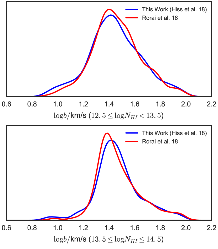
Figure 21.— Comparison of normalized $\log b$-distributions of data in Rorai et al. (2018) in the redshift bin $2.55\leq z\leq 2.95$ and this work in the redshift bin $2.7\leq z<2.9$.

Appendix B Comparison with Rorai et al. (2018)

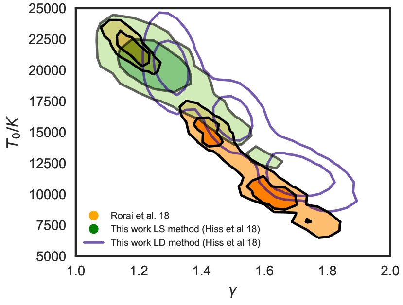
Figure 22.— Comparison of $T_{0}$ and $\gamma$ contours in Rorai et al. (2018) and this work (LS method in green, LD method in purple) at $z=2.8$. The contours correspond to the 68% and 95% confidence regions.

Recently, a study by Rorai et al. (2018) reported measurements of the thermal state of the IGM in the redshift interval $2.55\leq z\leq 2.95$ which resulted in values of $T_{0}$ and $\gamma$ that are only marginally consistent with our measurement at $2.7\leq z<2.9$. To test if the source of this discrepancy originates from the way in which the Voigt-profile algorithm was applied to the respective datasets, we plotted the line width distributions for both our line lists for two intervals of 1 dex in $N_{\text{\text{HI}}}$ within the cutoff fitting range. The distributions shown in Figure 21 are essentially identical. Thus, any difference in the resulting thermal parameters must originate in the cutoff fitting procedure due to contamination, spurious lines or differences in the calibration.

In Figure 22 a direct comparison of the contours of $T_{0}$ and $\gamma$ shows that Rorai et al. (2018) measures a multimodal joint distribution $p(T_{0},\gamma)$ (orange) while our measurement (green) recovers only the peak with the highest $T_{0}$ and lowest $\gamma$. The main difference between the two methods is that we perform a Least-square (LS) minimization fit at each iteration of the cutoff fitting procedure, while Rorai et al. (2018) performs a least absolute deviation (LD) fit. Our algorithm tends to converge to the peak corresponding to high $b_{0}$ and low $\Gamma$, resulting in this difference.

For comparison we re-run our measurements, this time applying a least absolute deviation fit for both our data and simulations. Due to unstable behavior of the least absolute deviation method at some redshifts, we applied no 2$\sigma$ outlier rejection (§ 2.3.2) to our data $b$-$N_{\text{HI}}$ distribution when applying this method. We show the resulting $p(T_{0},\gamma)$ contours at $z=2.8$ in purple in Figure 22. The results of the evolution of $T_{0}$ and $\gamma$ are shown in Figure 23. Essentially, the main difference between the two methods when applied to our data, is that we see extended uncertainties at $z=2.6$ and $z=2.8$, which originate from multimodal distributions $p(T_{0},\gamma)$. Furthermore, the redshift evolution of $\gamma$ is consistent with a constant $\gamma\simeq 1.4$.

As in Rorai et al. (2018), when using the least absolute deviation method, we observe a multimodal $p(T_{0},\gamma)$ distribution at $z=2.8$ (also at $z=2.6$) in the data that result from a multimodal $p(b_{0},\Gamma)$ measurement. When dealing with simulated $b$-$N_{\text{HI}}$ distributions both methods lead to unimodal solutions. This opens up the question if these multiple peaks in the inference of the cutoff parameters are a real feature due to multimodality in the temperature or an artifact of the cutoff fitting procedure due to unknown systematics in the data. Investigating the source of these structures is beyond the scope of this paper but we plan to study this in detail in the future.

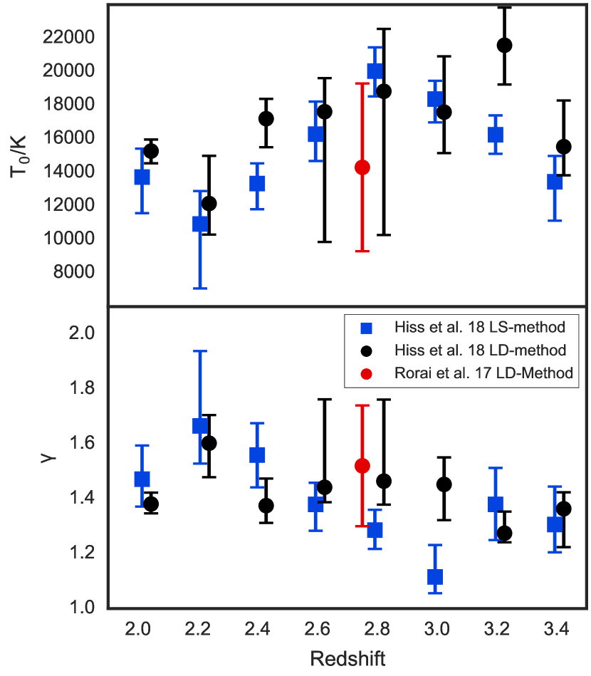
Figure 23.— Comparison of the marginalized $T_{0}$ and $\gamma$ in Rorai et al. (2018) (red) and this work (blue). We also ran our procedure using a least absolute deviation (LD) minimization cutoff fitting procedure (black). The main difference between the methods is that the least-squares (LS) minimization method used in this work does not show a multimodal structure at $z=2.6$ and $z=2.8$. Also the evolution of $\gamma$ is consistent with a constant, not showing a dip at $z=3$.

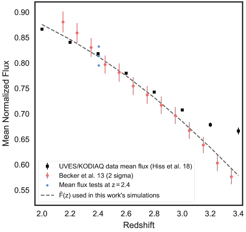
Figure 24.— Comparison of the mean flux evolution from Oñorbe et al. (2017) (dashed line, used as a basis for re-scaling the mock skewers in this work), the measurements by Becker et al. (2013) (red points) and the mean flux of the data used in this work at each redshift bin. The mean flux values used in for the test in Figure 25 are shown in blue.

Appendix C Impact of uncertainties in the mean flux

We describe in § 3 how our simulations are re-scaled in terms of flux in order to match the mean flux evolution fit $\bar{F}(z)$ from Oñorbe et al. (2017). This re-scaling is a standard procedure for accounting for our lack of knowledge of the precise value of the metagalactic ionizing background photoionization rate.

In Figure 24 we show a comparison of the mean flux values inferred from our data set (black squares), the values in Becker et al. (2013) (red) and the fit to diverse mean Flux measurements from Oñorbe et al. (2017) (dashed line) which was used as a basis for rescaling the mean flux of simulated spectra in this work. Only pixels that were not flagged as metals, high column density absorbers or bad pixels were used for the calculation of the mean flux in our data. When looking at the mean flux of data, we observe that they scatter around the mean flux used in the simulations in the range $z=2.0$ to 3.0.

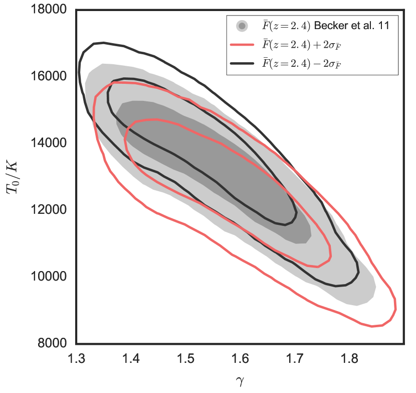
Figure 25.— Comparison of results at $z=2.4$ for our data calibrated using simulations that are scaled to three different mean flux values: Becker et al. (2011) mean Flux (gray filled contours), Becker et al. (2011) mean Flux +2$\sigma$ (red contour lines) and Becker et al. (2011) mean Flux -2$\sigma$ (black contour lines). The contours correspond to the 68% and 95% confidence regions.

To motivate the fact that we do not take into account uncertainties in the mean flux re-scaling of our simulations at $2<z<3$, we ran our measurements at $z=2.4$ for different values of the flux re-scaling: $\bar{F}$, i.e. our measurement, and $\bar{F}\pm 2\sigma_{\bar{F}}$, where $\bar{F}=0.8136$ is the value interpolated between the measurements of $\bar{F}$ by Becker et al. (2013) at $z=2.35$ and $z=2.45$. For the purpose of being conservative, the value of $\sigma_{\bar{F}}$ adopted is the error reported by Becker et al. (2013) at $z=2.35$, $\sigma_{\bar{F}}=0.0093$. These values are plotted as blue dots in Figure 24. The corresponding $p(T_{0},\gamma)$ measurements are shown in Figure 25. Shifting $\bar{F}$ by $2\sigma$ results in a negligible shift of our final results at this redshift.

At our highest redshift bins, $z=3.2$ and $z=3.4$ we observe a stronger discrepancy between the mean flux of our models and data. In order to directly examine the effect of this discrepancy on our measurements, we generated the models used in the calibration once again, with the difference that we re-scaled the optical depths to match the mean flux values measured in the data at these redshifts. We then applied the calibration based on these new models to our cutoff fit results. The results are shown in Figure 26. We observe that the calibrations at these redshifts are only slightly sensitive to this change, as our results basically do not change.

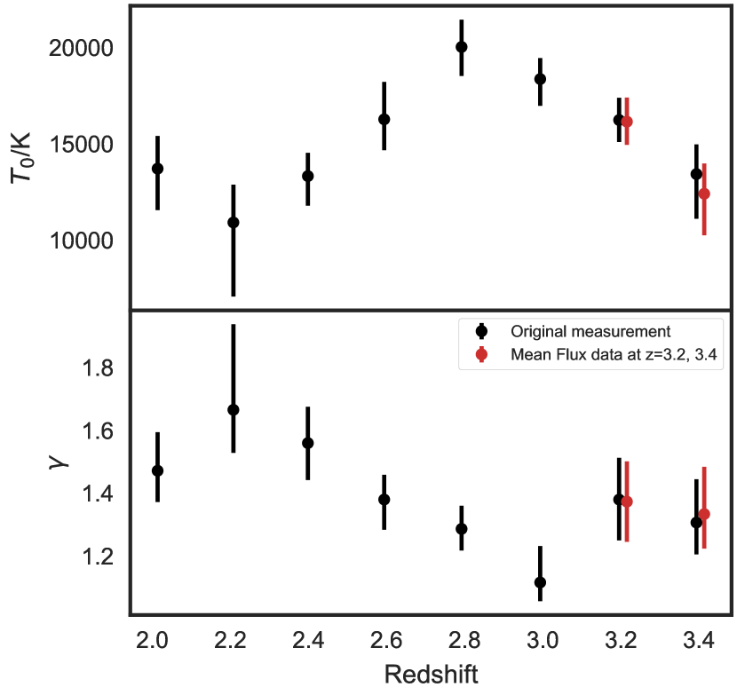
Figure 26.— Final marginalized $T_{0}$ and $\gamma$ measurements after re-scaling our models to match the mean flux of our data at $z=3.2$ and $z=3.4$ (red) compared to our original measurements (black).

References

- Almgren et al. (2013) Almgren, A. S., Bell, J. B., Lijewski, M. J., Lukić, Z., & Van Andel, E. 2013, ApJ, 765, 39
- Becker & Bolton (2013) Becker, G. D., & Bolton, J. S. 2013, MNRAS, 436, 1023
- Becker et al. (2011) Becker, G. D., Bolton, J. S., Haehnelt, M. G., & Sargent, W. L. W. 2011, MNRAS, 410, 1096
- Becker et al. (2013) Becker, G. D., Hewett, P. C., Worseck, G., & Prochaska, J. X. 2013, MNRAS, 430, 2067
- Boera et al. (2014) Boera, E., Murphy, M. T., Becker, G. D., & Bolton, J. S. 2014, MNRAS, 441, 1916
- Bolton et al. (2014) Bolton, J. S., Becker, G. D., Haehnelt, M. G., & Viel, M. 2014, MNRAS, 438, 2499
- Bolton et al. (2008) Bolton, J. S., Viel, M., Kim, T.-S., Haehnelt, M. G., & Carswell, R. F. 2008, MNRAS, 386, 1131
- Bryan & Machacek (2000) Bryan, G. L., & Machacek, M. E. 2000, ApJ, 534, 57
- Carswell & Webb (2014) Carswell, R. F., & Webb, J. K. 2014, VPFIT: Voigt profile fitting program, Astrophysics Source Code Library, ascl:1408.015
- Carswell et al. (2014) Carswell, R. F., Webb, J. K., Cooke, A. J., & Irwin, M. J. 2014, RDGEN: Routines for data handling, display, and adjusting, Astrophysics Source Code Library, ascl:1408.017
- Compostella et al. (2013) Compostella, M., Cantalupo, S., & Porciani, C. 2013, MNRAS, 435, 3169
- Dall’Aglio et al. (2008) Dall’Aglio, A., Wisotzki, L., & Worseck, G. 2008, AAP, 491, 465
- D’Aloisio et al. (2015) D’Aloisio, A., McQuinn, M., & Trac, H. 2015, ApJL, 813, L38
- Danforth et al. (2013) Danforth, C., Pieri, M., Shull, J. M., et al. 2013, in American Astronomical Society Meeting Abstracts, Vol. 221, American Astronomical Society Meeting Abstracts #221, 245.04
- Danforth et al. (2016) Danforth, C. W., Keeney, B. A., Tilton, E. M., et al. 2016, ApJ, 817, 111
- Dekker et al. (2000) Dekker, H., D’Odorico, S., Kaufer, A., Delabre, B., & Kotzlowski, H. 2000, in Society of Photo-Optical Instrumentation Engineers (SPIE) Conference Series, Vol. 4008, Optical and IR Telescope Instrumentation and Detectors, ed. M. Iye & A. F. Moorwood, 534–545
- Fan et al. (2006) Fan, X., Strauss, M. A., Becker, R. H., et al. 2006, AJ, 132, 117
- Faucher-Giguère et al. (2008a) Faucher-Giguère, C.-A., Lidz, A., Hernquist, L., & Zaldarriaga, M. 2008a, ApJ, 688, 85
- Faucher-Giguère et al. (2008b) Faucher-Giguère, C.-A., Prochaska, J. X., Lidz, A., Hernquist, L., & Zaldarriaga, M. 2008b, ApJ, 681, 831
- Gaikwad et al. (2017) Gaikwad, P., Srianand, R., Choudhury, T. R., & Khaire, V. 2017, MNRAS, 467, 3172
- Garzilli et al. (2012) Garzilli, A., Bolton, J. S., Kim, T.-S., Leach, S., & Viel, M. 2012, MNRAS, 424, 1723
- Gnedin & Hui (1998) Gnedin, N. Y., & Hui, L. 1998, MNRAS, 296, 44
- Haardt & Madau (2012) Haardt, F., & Madau, P. 2012, ApJ, 746, 125
- Haehnelt & Steinmetz (1998) Haehnelt, M. G., & Steinmetz, M. 1998, MNRAS, 298, L21
- Herbert-Fort et al. (2006) Herbert-Fort, S., Prochaska, J. X., Dessauges-Zavadsky, M., et al. 2006, PASP, 118, 1077
- Hiss et al. (2018) Hiss, H., Walther, M., Hennawi, J., et al. 2018, Results from Voigt profile fitting from Hiss et al. 2018, doi:10.5281/zenodo.1285569
- Hui & Gnedin (1997) Hui, L., & Gnedin, N. Y. 1997, MNRAS, 292, 27
- Hui & Rutledge (1999) Hui, L., & Rutledge, R. E. 1999, ApJ, 517, 541
- Katz et al. (1992) Katz, N., Hernquist, L., & Weinberg, D. H. 1992, ApJL, 399, L109
- Khaire et al. (2016) Khaire, V., Srianand, R., Choudhury, T. R., & Gaikwad, P. 2016, MNRAS, 457, 4051
- Kim et al. (2007) Kim, T.-S., Bolton, J. S., Viel, M., Haehnelt, M. G., & Carswell, R. F. 2007, MNRAS, 382, 1657
- Kim et al. (2004) Kim, T.-S., Viel, M., Haehnelt, M. G., Carswell, R. F., & Cristiani, S. 2004, MNRAS, 347, 355
- Kirkman et al. (2005) Kirkman, D., Tytler, D., Suzuki, N., et al. 2005, MNRAS, 360, 1373
- Kulkarni et al. (2015) Kulkarni, G., Hennawi, J. F., Oñorbe, J., Rorai, A., & Springel, V. 2015, Apj, 812, 30
- Lee et al. (2015) Lee, K.-G., Hennawi, J. F., Spergel, D. N., et al. 2015, ApJ, 799, 196
- Lehner et al. (2014) Lehner, N., O’Meara, J. M., Fox, A. J., et al. 2014, ApJ, 788, 119
- Lidz et al. (2010) Lidz, A., Faucher-Giguère, C.-A., Dall’Aglio, A., et al. 2010, ApJ, 718, 199
- Lukić et al. (2015) Lukić, Z., Stark, C. W., Nugent, P., et al. 2015, MNRAS, 446, 3697
- Madau & Haardt (2015) Madau, P., & Haardt, F. 2015, ApJL, 813, L8
- McDonald et al. (2001) McDonald, P., Miralda-Escudé, J., Rauch, M., et al. 2001, ApJ, 562, 52
- McGreer et al. (2015) McGreer, I. D., Mesinger, A., & D’Odorico, V. 2015, MNRAS, 447, 499
- McQuinn (2016) McQuinn, M. 2016, ARAA, 54, 313
- McQuinn et al. (2009) McQuinn, M., Lidz, A., Zaldarriaga, M., et al. 2009, Apj, 694, 842
- McQuinn & Upton Sanderbeck (2016) McQuinn, M., & Upton Sanderbeck, P. R. 2016, MNRAS, 456, 47
- Meiksin (2009) Meiksin, A. A. 2009, Reviews of Modern Physics, 81, 1405
- Nasir et al. (2017) Nasir, F., Bolton, J. S., Viel, M., et al. 2017, MNRAS, 471, 1056
- Oñorbe et al. (2017) Oñorbe, J., Hennawi, J. F., & Lukić, Z. 2017, ApJ, 837, 106
- O’Meara et al. (2017) O’Meara, J. M., Lehner, N., Howk, J. C., et al. 2017, ArXiv e-prints, arXiv:1707.07905
- O’Meara et al. (2015) —. 2015, ArXiv e-prints, arXiv:1505.03529
- O’Meara et al. (2016) —. 2016, VizieR Online Data Catalog, 515
- Palanque-Delabrouille et al. (2013) Palanque-Delabrouille, N., Yèche, C., Borde, A., et al. 2013, AAP, 559, A85
- Planck Collaboration et al. (2014) Planck Collaboration, Ade, P. A. R., Aghanim, N., et al. 2014, AAP, 571, A16
- Puchwein et al. (2015) Puchwein, E., Bolton, J. S., Haehnelt, M. G., et al. 2015, MNRAS, 450, 4081
- Ricotti et al. (2000) Ricotti, M., Gnedin, N. Y., & Shull, J. M. 2000, ApJ, 534, 41
- Robertson et al. (2015) Robertson, B. E., Ellis, R. S., Furlanetto, S. R., & Dunlop, J. S. 2015, ApJL, 802, L19
- Rorai et al. (2018) Rorai, A., Carswell, R. F., Haehnelt, M. G., et al. 2018, MNRAS, 474, 2871
- Rorai et al. (2013) Rorai, A., Hennawi, J. F., & White, M. 2013, ApJ, 775, 81
- Rorai et al. (2017a) Rorai, A., Becker, G. D., Haehnelt, M. G., et al. 2017a, MNRAS, 466, 2690
- Rorai et al. (2017b) Rorai, A., Hennawi, J. F., Oñorbe, J., et al. 2017b, Science, 356, 418
- Rudie et al. (2012a) Rudie, G. C., Steidel, C. C., & Pettini, M. 2012a, ApJ, 757, L30
- Rudie et al. (2012b) Rudie, G. C., Steidel, C. C., Trainor, R. F., et al. 2012b, ApJ, 750, 67
- Schaye (2001) Schaye, J. 2001, Apj, 559, 507
- Schaye et al. (1999) Schaye, J., Theuns, T., Leonard, A., & Efstathiou, G. 1999, MNRAS, 310, 57
- Schaye et al. (2000) Schaye, J., Theuns, T., Rauch, M., Efstathiou, G., & Sargent, W. L. W. 2000, MNRAS, 318, 817
- Theuns et al. (2002) Theuns, T., Schaye, J., Zaroubi, S., et al. 2002, ApJl, 567, L103
- Upton Sanderbeck et al. (2016) Upton Sanderbeck, P. R., D’Aloisio, A., & McQuinn, M. J. 2016, MNRAS, 460, 1885
- Viel et al. (2009) Viel, M., Bolton, J. S., & Haehnelt, M. G. 2009, MNRAS, 399, L39
- Viel et al. (2017) Viel, M., Haehnelt, M. G., Bolton, J. S., et al. 2017, MNRAS, 467, L86
- Vogt et al. (1994) Vogt, S. S., Allen, S. L., Bigelow, B. C., et al. 1994, in Society of Photo-Optical Instrumentation Engineers (SPIE) Conference Series, Vol. 2198, Instrumentation in Astronomy VIII, ed. D. L. Crawford & E. R. Craine, 362
- Walther et al. (2018) Walther, M., Hennawi, J. F., Hiss, H., et al. 2018, ApJ, 852, 22
- White et al. (2002) White, M., Hernquist, L., & Springel, V. 2002, ApJ, 579, 16
- Worseck et al. (2011) Worseck, G., Prochaska, J. X., McQuinn, M., et al. 2011, ApJl, 733, L24
- Zaldarriaga et al. (2001) Zaldarriaga, M., Hui, L., & Tegmark, M. 2001, ApJ, 557, 519