Inside-Out Planet Formation. IV. Pebble Evolution and Planet Formation Timescales

Abstract

Systems with tightly-packed inner planets (STIPs) are very common. Chatterjee & Tan (2014) proposed Inside-Out Planet Formation (IOPF), an in situ formation theory, to explain these planets. IOPF involves sequential planet formation from pebble-rich rings that are fed from the outer disk and trapped at the pressure maximum associated with the dead zone inner boundary (DZIB). Planet masses are set by their ability to open a gap and cause the DZIB to retreat outwards. We present models for the disk density and temperature structures that are relevant to the conditions of IOPF. For a wide range of DZIB conditions, we evaluate the gap opening masses of planets in these disks that are expected to lead to truncation of pebble accretion onto the forming planet. We then consider the evolution of dust and pebbles in the disk, estimating that pebbles typically grow to sizes of a few cm during their radial drift from several tens of AU to the inner, $\lesssim 1\>$AU-scale disk. A large fraction of the accretion flux of solids is expected to be in such pebbles. This allows us to estimate the timescales for individual planet formation and entire planetary system formation in the IOPF scenario. We find that to produce realistic STIPs within reasonable timescales similar to disk lifetimes requires disk accretion rates of $\sim 10^{-9}\>M_{\odot}\>{\rm yr}^{-1}$ and relatively low viscosity conditions in the DZIB region, i.e., Shakura-Sunyaev parameter of $\alpha\sim 10^{-4}$.

1. Introduction

More than 4000 exoplanet candidates (e.g., Mullally et al., 2015) have been discovered by Kepler since 2009, a significant percentage ($\gtrsim 30\%$) of which are in systems with tightly-packed inner planets (hereafter STIPs). STIPs are very different from our Solar System: they typically contain three or more detected planets of radii $\sim 1-10\>R_{\oplus}$ and with periods less than 100 days (Fang & Margot, 2012), i.e., with orbital radii of $\lesssim 0.3$ AU.

One way to form STIPs may be via inward migration of planets formed in the outer disk (e.g., Kley & Nelson, 2012; Cossou et al., 2013, 2014). However, it can be quite difficult to concentrate planets close to the host star to the degree of observed STIPs (McNeil & Nelson, 2010). Also migrating planets tend to become trapped in orbits of low order mean motion resonances, which is not a particular feature of STIPs (Baruteau et al., 2014; Fabrycky et al., 2014). This lack of resonant pile-up has motivated studies of mechanisms that cause a lower efficiency of resonance trapping (Goldreich & Schlichting, 2014) or breaking of resonance by later dynamical interaction with, e.g., a planetesimal disk (Chatterjee & Ford, 2015), by the unstable nature of compact resonant chains (Izidoro et al., 2017), or by magnetospheric rebound from the host star during gas disk dispersal (Liu et al., 2017).

As an alternative to inward migration, in situ formation scenarios (Hansen & Murray, 2012, 2013) have considered a group of protoplanets that are initially distributed inside 1 AU with high concentration. After following dynamical evolution for 10 Myr, collisional oligarchic growth can lead to systems quite similar to STIPs. However, how this initial condition was established was not well studied in these works and may be subject to some difficulties, such as early triggering of gravitational instability (Raymond & Cossou, 2014; Schlichting, 2014) (see also, Chiang & Laughlin, 2013). In addition, simulations that account for the effects of gas on protoplanet migration during the oligarchic growth phase find that systems are produced with planet masses decreasing steeply with orbital radius, which is different from the relatively flat scaling seen in STIPs (Ogihara et al., 2015).

The Inside-Out Planet Formation (IOPF) scenario proposed by (Chatterjee & Tan, 2014, hereafter Paper I) is a new type of in situ formation model. It starts with pebble delivery to the disk midplane transition region between an innermost magnetorotational instability (MRI) active zone and a nonactive “dead zone,” where there is a local pressure maximum. The pebbles are trapped here and build up in a ring, which then forms a first protoplanet, perhaps involving a variety of processes including streaming (Youdin & Goodman, 2005), gravitational (Toomre, 1964) and/or Rossby wave (Varnière & Tagger, 2006) instabilities. The protoplanet is expected to continue its growth, especially by pebble accretion, until it becomes massive enough to open a gap in the disk. This gap, which may only be a partial gap with a modest reduction in gas mass surface density, pushes the pressure maximum outwards by at least a few Hill radii from the first planet, thus creating a new pebble trap, and thus location of second planet formation (Hu et al., 2016, hereafter Paper III) (see also Lambrechts et al., 2014). Furthermore, MRI-activation in this gap region beyond the first planet may induce enhanced viscosity and thus further outward retreat of the dead zone inner boundary (DZIB) pressure trap, leading to larger separations to the orbit of the second planet.

The pebble delivery rate is crucial for setting the timescale of pebble ring and planet formation in the IOPF scenario. To calculate this, we need to model the evolution of dust and pebbles in the protoplanetary disk and determine if the majority of solid material, which in the outer disk is initially in small dust grains, become incorporated into pebbles by the time it reaches the inner region. The IOPF model requires dust grains to grow into pebbles as smaller grains are well coupled to the gas and will not be trapped at a local pressure maximum (e.g., Zhu et al., 2012). The size distribution of pebbles is also important for models of planetesimal formation, e.g., via the streaming instability. This may be triggered in both the pebble ring as a first step for in situ planet formation, or in the outer disk as a potential first step for outer planet formation that may eventually truncate pebble delivery to the inner disk. Finally, modeling of dust and pebble evolution is a necessary step for then providing observational predictions of the emission from the disk during various phases of IOPF.

There have been a number of previous studies of dust and pebble evolution in global disk models, including radial drift and particle interaction (e.g., Brauer et al., 2008; Birnstiel et al., 2010). Birnstiel et al. (2012) proposed a two population model that divides dust into one smaller fixed size group and one larger variable size group that represents grain growth. Sato et al. (2015) proposed a simplified pebble-pebble interaction scenario by reducing the full Smoluchowski equation to a single sized evolution equation, yielding pebble fluxes and typical sizes in disks on scales down to $\sim$1 AU. A Lagrangian dust evolution model has been investigated by Krijt et al. (2016), which tracks batches of particles in the disk as they drift radially and grow through collisions.

In this paper, we present a new pebble-dust evolution model and apply it specifically to calculate the timescales needed to build up a STIP forming via IOPF, i.e., limited by the rate of pebble delivery. In §2, we review the equations that govern the disk models that are relevant to IOPF, including presenting new disk structure models that include realistic opacities and the transition from an “active,” accretion-powered inner disk to a “passive,” stellar-heated outer disk. In §3, we discuss a simple estimate of the timescale of first, so-called “Vulcan” planet formation in steady accretion rate disks, including a reanalysis of the gap-opening mass criterion that was studied in Paper III. We also estimate the size of the region of the disk that is needed to supply the material for this planet. In §4, we model the radial drift and sweep up growth of a single pebble in our model disks. In §5, we introduce our full pebble evolution model and numerical results for different disk parameters. In §6 we outline the assembly of a STIPs-like system with pebble flux and planet mass criterion derived from earlier sections. We discuss the implications of our results and summarize our conclusions in §7.

2. Disk Structure

The structure of a steady accretion disk can be specified with a given accretion rate $\dot{m}$, Shakura & Sunyaev (1973) viscosity parameter $\alpha$, stellar mass $m_{*}$, and midplane temperature versus radius relation $T(r)$ (in particular specifying whether the energy source of the disk is heating mostly by its own accretion, i.e., an “active” disk, or whether it is heating mostly by stellar irradiation, i.e., a “passive” disk):

$$T = T(r)$$ (1)

$$c_{s} = (\gamma k_{B}T/\mu)^{1/2}$$ (2)

$$h/r = c_{s}/v_{K}$$ (3)

$$\nu = \alpha c_{s}h$$ (4)

$$\Sigma_{g} = \dot{m}/(3\pi\nu)$$ (5)

$$\rho = \Sigma_{g}/(h\sqrt{2\pi}),$$ (6)

where $c_{s}$ is the midplane sound speed, $\gamma$ is the power law exponent of the barotropic equation of state $P=K\rho^{\gamma}$, $k_{B}$ is Boltzmann’s constant, $\mu=2.33m_{\rm{H}}=3.90\times 10^{-24}\>\rm{g}$ is the mean particle mass (with fiducial value set by assuming $n_{\rm He}=0.2n_{\rm H2}$), $h$ is the disk vertical scaleheight, $v_{K}$ is the local Keplerian speed, $\nu$ is the viscosity, $\alpha\equiv 10^{-4}\alpha_{-4}$ is the Shakura-Sunyaev dimensionless viscosity parameter (with fiducial value set for dead zone conditions, but we will consider other values also), $\Sigma_{g}$ is the gas mass surface density, $\dot{m}\equiv\dot{m}_{-9}10^{-9}\>M_{\odot}\>{\rm yr}^{-1}$ is the accretion rate (with fiducial normalization set by observed accretion rates of transition disks, but again we will consider a range of values; see Paper I) and $\rho$ is midplane gas density. Only equations (1) and (2) depend on the energy source and equation of state, while the rest are general equations followed by all viscous disks.

The solution for the structure of an active accretion disk is achieved by balancing viscous thermal dissipation with vertical radiative cooling (per unit area from one face of the disk):

$$\frac{\nu\Sigma_{g}r^{2}}{2}\left(\frac{d\Omega}{dr}\right)^{2}=\frac{16\sigma_{\rm SB}}{3\Sigma_{g}\kappa}T^{4}$$ (7)

This generally applies in the inner disk. In this case the temperature equation is (Paper I):

$$T = \frac{3^{1/5}}{2^{7/5}\pi^{2/5}}\left(\frac{\mu}{\gamma k_{B}}\right)^{1/5}\left(\frac{\kappa}{\sigma_{\rm SB}}\right)^{{1}/{5}}$$

$$\times \alpha^{-1/5}\left(Gm_{*}\right)^{3/10}\left(f_{r}\dot{m}\right)^{2/5}r^{-{9}/{10}},$$

$$\rightarrow 290\gamma_{1.4}^{-1/5}\kappa_{10}^{1/5}\alpha_{-4}^{-1/5}m_{*,1}^{3/10}(f_{r}\dot{m}_{-9})^{2/5}r_{\rm AU}^{-9/10}\>\rm K,$$

and gas mass surface density is given by:

$$\Sigma_{g} = \frac{2^{7/5}}{3^{6/5}\pi^{3/5}}\left(\frac{\mu}{\gamma k_{B}}\right)^{4/5}\left(\frac{\kappa}{\sigma_{\rm SB}}\right)^{-{1}/{5}}$$

$$\times \alpha^{-4/5}\left(Gm_{*}\right)^{1/5}\left(f_{r}\dot{m}\right)^{3/5}r^{-{3}/{5}},$$

$$\rightarrow 812\gamma_{1.4}^{-4/5}\kappa_{10}^{-1/5}\alpha_{-4}^{-4/5}m_{*,1}^{1/5}(f_{r}\dot{m}_{-9})^{3/5}{r_{\rm AU}}^{-3/5}\>\rm g\>cm^{-2},$$

where $\gamma\equiv 1.4\gamma_{1.4}$ with fiducial normalization to a value of 1.4 for $\rm H_{2}$ with rotational modes excited, $\kappa\equiv\kappa_{10}10\ {\rm cm^{2}\>g^{-1}}$ is the disk mean opacity (with fiducial normalization here appropriate for inner disk conditions; but, note we will more generally use tabulated opacities from Zhu et al., 2009), $\sigma_{\rm SB}$ is the Stefan-Boltzmann constant, $m_{*}\equiv m_{*,1}M_{\odot}$ is the stellar mass with fiducial normalization of $1\>M_{\odot}$, $f_{r}\equiv 1-\sqrt{r_{*}/r}$, $r_{*}$ is the stellar radius, and $r_{\rm AU}\equiv r/(1\>{\rm AU})$. The two parameters with some of the largest uncertainties are $\alpha$ and $\dot{m}$, so we shall consider the effects of varying their fiducial values.

In the outer disk, stellar irradiation is expected to become the dominant energy source compared to local viscous accretion heating. Following Chiang & Goldreich (1997), the temperature structure of a stellar irradiated, passive disk follows $T\propto r^{-3/7}$, which is much shallower than the $T\propto r^{-9/10}$ relation of the active disk.

To derive $T(r)$ in the passive disk regime, the following equations are solved iteratively:

$$T = (\beta/4)^{1/4}(r_{*}/r)^{1/2}T_{\rm*,eff};$$ (10)

$$\beta = 0.4r_{*}/r+\eta H/r.$$ (11)

Here $\beta$ is the “grazing angle,” i.e., the angle of incidence of stellar radiation at the disk surface, $T_{\rm*,eff}$ is the surface, photospheric temperature of the star, $\eta=2/7$ is the flaring index, i.e., $\eta=d(h/r)/dr$, and $H$ is the height of the disk photosphere above the midplane. Usually, $H=4h$ is a good approximation in most parts of the disk (Chiang & Goldreich, 1997). If we choose a solar mass T-Tauri star with temperature $T_{\rm*,eff}=4500\>K$ and radius $r_{*}=3.0\>R_{\odot}=0.014\rm AU$, we have the disk temperature versus radius equation

$$T = 172r_{\rm AU}^{-3/7}\>\rm K,$$ (12)

which is independent of $\alpha$ and $\dot{m}$.

For our full numerical solutions, we set up a hybrid disk that is solved first in its inner region as an active disk, and then calculate a transition radius where the contribution from stellar irradiation becomes equal to that due to accretion heating. Beyond this transition radius, we scale the temperature in the manner appropriate for the passive disk regime, i.e., in particular, we compare the midplane temperatures of the active and passive disk models and choose the hotter one as the actual value.

The results of these constant $\alpha=10^{-4}$ (the fiducial value) and $10^{-3}$ and constant $\dot{m}=10^{-10}$, $10^{-9}$ and $10^{-8}\>M_{\odot}\>{\rm yr}^{-1}$ disk models are shown in Figure 1. Such values of $\alpha$ have been inferred in the inner regions of simulated dead zones (Dzyurkevich et al., 2010). Whether such dead zone conditions and values of $\alpha$ continue to apply in larger scale regions of the disk remains an open question (e.g., Mohanty et al., 2013), however, for simplicity we will assume that they do and calculate the structure of the disk out to 30 AU. The range of accretion rates that we consider is guided by observations of transition disks (e.g., Manara et al., 2014). Another risk of applying constant $\alpha$ and stable accreting disk to larger radius is overestimating the disk mass. In our fiducial case, as seen in Figure 1, the dust mass within 30 AU is about 100 $M_{\oplus}$, while recent observations on dust continuum (van der Marel et al., 2016) give an average around 40 $M_{\oplus}$ for most transitional disks. This factor of 2 should be considered when analyzing the simulation result. The active to passive transition radius for the fiducial disk ($\dot{m}=10^{-9}M_{\odot}\>{\rm yr}^{-1},\alpha=10^{-4}$) is 1.6 AU. We note that the model assumption of disk vertical optical depth being $\gtrsim 1$ breaks down in the cases with $\alpha=10^{-3}$ and $\dot{m}\leq 10^{-9}\>M_{\odot}\>{\rm yr}^{-1}$ in the outer disk, e.g., for $\dot{m}=10^{-9}\>M_{\odot}\>{\rm yr}^{-1}$ this occurs for $r>8.5$ AU. Note also that an “inner transition” in disk structure at 0.14 AU results from the drop in opacity due to dust sublimation. However, in the context of IOPF, we expect $\alpha$ to also rise dramatically when $T\sim 1200\>$K (this location is referred as $r_{\rm 1200K}$ hereafter) as the MRI is activated by thermal ionization of alkali metals. This change in $\alpha$ has not been included in the models shown in Fig. 1 since our main focus here is modeling the region that is the supply reservoir for solid material delivered to $\sim$0.1 AU locations. Still, we have extended the disk models within 0.1 AU, since for the low accretion rate case ($\dot{m}=10^{-10}M_{\odot}\>{\rm yr}^{-1}$), $r_{\rm 1200K}<0.1\>\rm AU$.

In fact, there are some close-in planets with orbits within 0.1 AU, e.g., Kepler-10b (Dumusque et al., 2014) is a super-Earth planet orbiting a solar type star at 0.016 AU. For such planets to form in situ places constraints on IOPF models. For example, such systems would need to form in a disk with relatively low accretion rate that has a small value of $r_{\rm 1200K}$ (see below).

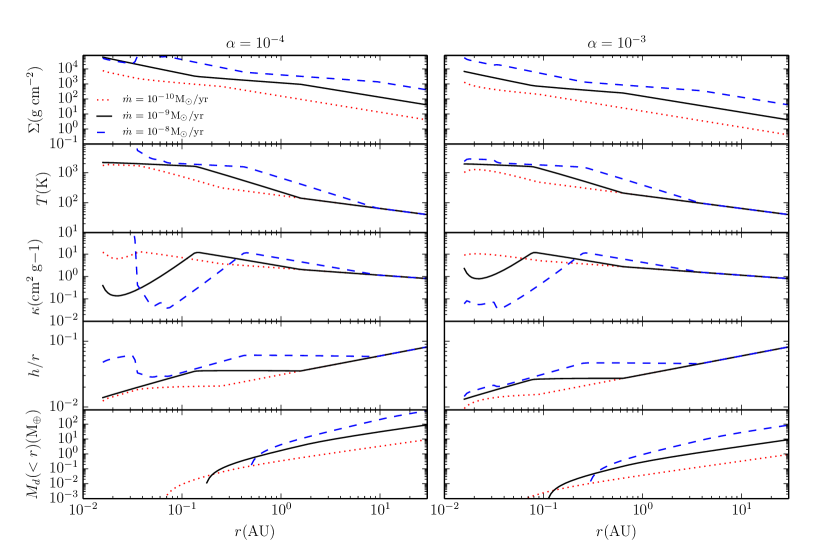
Figure 1.— Structural profiles of IOPF disk models used in this paper, assuming $\alpha=10^{-4}$ (left column) and $\alpha=10^{-3}$ (right column), for accretion rates $10^{-10}$ (red dotted), $10^{-9}$ (black solid) and $10^{-8}\>M_{\odot}\>{\rm yr}^{-1}$ (blue dashed). All models are for a one solar mass central star. From top to bottom, the rows show: gas mass surface density ($\Sigma_{g}$); midplane temperature ($T$); midplane opacity ($\kappa$) (assumed to be vertically constant); disk aspect ratio ($h/r$); enclosed mass in solids ($M_{d}(<r)$), i.e., initially assumed to be dust, summed in the disk from $r_{\rm 1200K}$ out to radius $r$ for a solid to gas mass ratio of $f_{s}=0.01$. Note that the model assumption of disk vertical optical depth being $\gtrsim 1$ breaks down in the cases with $\alpha=10^{-3}$ and $\dot{m}\leq 10^{-9}\>M_{\odot}\>{\rm yr}^{-1}$ in the outer disk, e.g., for $\dot{m}=10^{-9}\>M_{\odot}\>{\rm yr}^{-1}$ this occurs at $r>8.5$ AU.

3. “Vulcan” planet formation

Our goal in this section is to obtain a simple estimate for the formation time and the size of the supply reservoir of the first, i.e., innermost planet to form in the IOPF scenario (Chatterjee & Tan, 2015, hereafter Paper II). To do this requires knowing the mass of such planets and the mass flux of pebbles. Here we will assume a steady accretion rate with most mass flux of solids being in the form of pebbles. The validity of this assumption will be explored in the following sections of the paper.

3.1. Location

The radial location of Vulcan planet formation is assumed to be set by where the temperature reaches $\sim$1,200 K that leads to thermal ionization of alkali metals, especially Na and K. This location varies depending on the accretion rate and other disk properties. In an active accretion disk, which is the relevant regime for the optically thick inner disk, this location is (Paper I):

$$r_{1200{\rm K}}=0.218\phi_{\rm DZIB}\gamma_{1.4}^{-2/9}\kappa_{10}^{2/9}\alpha_{-4}^{-2/9}m_{*,1}^{1/3}(f_{r}\dot{m}_{-9})^{4/9}\>{\rm AU},$$ (13)

where $\phi_{\rm DZIB}$ is a dimensionless parameter of order unity to account for potential differences from the pure viscous disk model, e.g., due to the effects of extra energy extraction on midplane temperature by a disk wind. Paper I and II adopted a fiducial value of $\phi_{\rm DZIB}$ of 0.5. In Paper III, we used 0.1 AU as the typical location of Vulcan planets for hydrodynamic simulations of gap opening, where $\alpha=10^{-3}$, $\dot{m}=10^{-9}\>M_{\odot}\>{\rm yr}^{-1}$, which corresponds to $\phi_{\rm DZIB}=0.76$.

3.2. Mass

The mass of the Vulcan planet (and all planets forming via IOPF) is assumed to be set by gap opening, which then leads to displacement of the local pressure maximum away from the planet, to a larger radius in the disk, and thus the truncation of pebble accretion. Paper III investigated this process with 2D hydrodynamic simulations for the case of the fiducial accretion rate ($10^{-9}\>M_{\odot}\>{\rm yr}^{-1}$), a value of $\alpha=10^{-3}$ for the inner dead zone that then rises to $\alpha=10^{-2}$ in the MRI-active region, and for the planet set at a fixed location of 0.1 AU from a $1\>M_{\odot}$ star. The mass of the planet leading to the first significant displacement of the pressure maximum was assessed relative to the viscous thermal criterion gap opening mass of Lin & Papaloizou (1993):

$$M_{G} = \phi_{G}\frac{40\nu m_{*}}{r^{2}\Omega_{K}}$$

$$= 40\phi_{G}\left(\frac{3}{128}\right)^{1/5}\pi^{-{2}/{5}}\left(\frac{\mu}{k_{B}}\right)^{-{4}/{5}}\gamma^{{4}/{5}}\sigma_{\rm SB}^{-{1}/{5}}$$

$$\times \alpha^{{4/5}}G^{-{7/10}}m_{*}^{{3}/{10}}\kappa^{1/5}\left(f_{r}\dot{m}\right)^{2/5}r^{{1}/{10}}$$

$$\rightarrow 11.2\phi_{G}\gamma_{1.4}^{4/5}\kappa_{10}^{1/5}\alpha_{-3}^{4/5}m_{*,1}^{3/10}(f_{r}\dot{m}_{-9})^{2/5}r_{\rm 0.1AU}^{1/10}\>M_{\oplus}$$

$$\rightarrow 1.77\phi_{G}\gamma_{1.4}^{4/5}\kappa_{10}^{1/5}\alpha_{-4}^{4/5}m_{*,1}^{3/10}(f_{r}\dot{m}_{-9})^{2/5}r_{\rm 0.1AU}^{1/10}\>M_{\oplus}.$$

Here $r_{\rm 0.1AU}\equiv r/(0.1\>{\rm AU})$. The last two numerical evaluations of this mass illustrate its relatively strong dependence on $\alpha$. Paper III found that, for the $\alpha=10^{-3}$ case, the critical pressure-displacement gap opening mass was about 50% of the viscous-thermal gap opening mass (i.e., this fraction was expressed as $\phi_{G}\simeq 0.5$). Note that the mass evaluated in equation (3.2) is assessed only from the viscous criterion, but, for the conditions with $\alpha=10^{-3}$, is consistent with the thermal criterion also, i.e., the Hill radius of the planet is similar in size to the disk scale height. However, as we see now, this condition breaks down when $\alpha=10^{-4}$, as the planet mass is much lower.

To better capture the behavior of gap opening for more general conditions in which the thermal criterion also begins to limit gap opening, we now improve our treatment by adopting the expression of Duffell (2015) for the gap opening mass (same scalings of $h/r$ and $\alpha$ is also presented in Zhu et al. (2013) and Fung et al. (2014)):

$$M_{\rm G,D} = \phi_{\rm G,D}\sqrt{3\pi}m_{*}\alpha^{1/2}\left(h/r\right)^{5/2}$$

$$= \phi_{\rm G,D}\frac{3^{3/4}}{2^{7/4}}\left(\frac{\mu}{\gamma k_{B}}\right)^{-1}\left(\frac{\kappa}{\sigma_{\rm SB}}\right)^{{1}/{4}}\alpha^{1/4}$$

$$\times G^{-7/8}m_{*}^{1/8}\left(f_{r}\dot{m}\right)^{1/2}r^{{1}/{8}},$$

$$\rightarrow 2.68\phi_{\rm G,D}\gamma_{1.4}\kappa_{10}^{1/4}\alpha_{-4}^{1/4}m_{*,1}^{1/8}(f_{r}\dot{m}_{-9})^{1/2}r_{\rm 0.1AU}^{1/8}\>\rm M_{\oplus}$$

where $\phi_{\rm G,D}$ is a dimensionless parameter of order unity (note this absorbs the dimensionless factor, $f_{0}$, introduced by Duffell (2015)). Note that the scaling of this relation is slightly different from the pebble isolation mass in Lambrechts et al. (2014), which depends on $h/r$, but not $\alpha$. However, a more recent prescription for the pebble isolation mass in Bitsch et al. (2018) also includes a dependence on $\alpha$. A major difference of our results from these other studies is that our planet gap opening mass measurements are done specifically at a region in the disk where there is a transition in the value of $\alpha$ that causes a strong change in $\Sigma$. On the other hand, the results of Lambrechts et al. (2014) and Bitsch et al. (2018) are for disks with constant $\alpha$ and thus a relatively slowly varying $\Sigma_{g}$ profile.

To test equation (3.2) and constrain $\phi_{\rm G,D}$, we now extend the simulations of Paper III to investigate the gap opening mass for different values of $\alpha$ and $\dot{m}$. We perform a series of FARGO (Masset, 2000) hydrodynamic simulations on disks with an $\alpha$ viscosity transition. The inner region is still assumed to be an MRI-active zone with $\alpha=0.01$. Beyond this is the dead zone with a much lower value of $\alpha$. We implement the transition following the same methods as Paper III, with the transition set to be at 0.1 AU, which is the location of the local pressure maximum before the introduction of a planet in the disk. Then planets of different masses are inserted in the disk and held fixed at this location (note Paper III showed that growing planets would be trapped here given the torques exerted by the disk). We study the cylindrically averaged pressure profiles and identify the critical gap-opening mass for IOPF as corresponding to the point when the local pressure maximum in the disk becomes significantly displaced from the planet, i.e., by more than its Hill radius,

$$R_{H} \equiv \left(\frac{M_{p}}{3m_{*}}\right)^{1/3}r$$

$$\rightarrow 1.00\times 10^{-3}M_{p,\oplus}^{1/3}m_{*,1}^{-1/3}r_{\rm 0.1AU}\>{\rm AU},$$

where $M_{p,\oplus}\equiv M_{p}/M_{\oplus}$ is the planet mass normalized to one Earth mass.

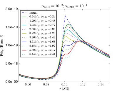
Figure 2.— Steady state, cylindrically averaged disk midplane pressure profiles, starting with an initial case with no planet. The pressure maximum, due to the dead zone inner boundary, has been set at 0.1 AU. We set $\alpha=0.01$ in the inner MRI-active disk, transitioning to $10^{-4}$ in the dead zone. Then the effects of adding planets of increasing mass and held fixed at 0.1 AU are studied. These planets open gaps of increasing depth, which eventually leads to displacement of the local pressure maximum away from the planet. This occurs for $M_{p}=3.86\>M_{\oplus}$, i.e., $\phi_{\rm G,D}=1.44$.

Figure 2 shows examples of these pressure profiles for the case of a disk with $\dot{m}=10^{-9}\>M_{\odot}\>{\rm yr}^{-1}$ and a transition from $\alpha=10^{-2}$ to $\alpha=10^{-4}$ in the vicinity of 0.1 AU. We see in this case that a planet with mass of $3.86\>M_{\oplus}$ is able to open a deep enough gap that the local pressure maximum retreats significantly, i.e., by $\sim 0.015\>$AU (in this case, $\sim 10$ Hill radii) from the planet. This mass scale corresponds to a value of $\phi_{\rm G,D}=1.44$ in the normalization of the Duffell (2015) gap opening mass (eq. 3.2). In the IOPF model this means that the next planet may form from a new pebble ring at this location or somewhat further out if the MRI-active region also spreads outwards in the lower densities enabled by gap opening.

Figure 3a shows the results of four different series of simulations, including the example shown in Fig. 2, in which $\alpha$ in the dead zone is varied from $10^{-4}$ to $10^{-3}$ and the gap opening masses (by the pressure maximum displacement criterion) are assessed and compared to those predicted by the simple viscous criterion (eq. 3.2) and the Duffell (2015) estimate (eq. 3.2). Figure 3b shows the results of a similar series of gap opening simulations, but now varying $\dot{m}$ from $10^{-10}$ to $10^{-7}\>M_{\odot}\>{\rm yr}^{-1}$. We find the simple viscous criterion underestimates the planet mass required for displacing the pressure maximum in both the low $\alpha$ and high $\dot{m}$ regimes. These are conditions when the disk is relatively denser and hotter and its vertical scale height is relatively large compared to the Hill sphere of the planet. Our results are consistent with those of Duffell & MacFadyen (2013): they discuss how gap profiles scale differently when a planet’s Hill radius is smaller than the disk scale height. We note that our results are derived from 2D simulations, which should ideally be confirmed by 3D simulations that resolve the vertical structure of the disk to more accurately predict midplane pressure structures.

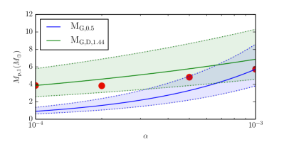
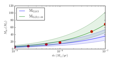
Figure 3.— Planet gap opening mass estimates based on the viscous criterion ($M_{G,0.5}$, blue) and the Duffell (2015) criterion ($M_{\rm G,D}$, green) as a function of viscosity $\alpha$ (top panel) and accretion rate $\dot{m}$ (bottom panel). The shaded area indicates a range of a factor of 1.5 variation about the fiducial mass estimates. The red dots are FARGO simulation results based on local pressure maximum retreat. Note the Duffell (2015) criterion is a better match with the simulation results in the low $\alpha$ and high $\dot{m}$ regimes.

With our improved estimate of Vulcan planet mass set by gap opening (eq. 3.2), following Paper II, we eliminate the accretion rate term, $f_{r}\dot{m}_{-9}$, by combining it with equation 13. Previously Paper II did this using the viscous criterion gap opening mass to obtain $M_{p,1}=0.83\phi_{G,0.5}\phi_{\rm DZIB,0.5}^{-9/10}\gamma_{1.4}\alpha_{-4}r_{\rm 0.1AU}\>M_{\oplus}$. Now we find a revised mass versus orbital radius relation for Vulcans:

$$M_{p,1} = 3.50\phi_{\rm G,D,1.44}\phi_{\rm DZIB,0.5}^{-9/8}\gamma_{1.4}^{5/4}$$ (17)

$$\times \alpha_{-4}^{1/2}m_{*,1}^{-1/4}r_{\rm 0.1AU}^{5/4}\>M_{\oplus}.$$

We see that this has a slightly steeper scaling of $M_{p,1}\propto r^{5/4}$ compared to the Paper II result. The implications of this and other revised IOPF predictions, such as the more general $M_{p}$ versus $r$ relation of eq. (3.2), for the comparison with observed STIPs will be examined in a future paper.

3.3. Formation Timescale

Now that we have improved estimates for the masses of Vulcan planets, we assess their formation timescales. Consider a protoplanetary disk with mass accretion rate of $\dot{m}$ and solids to gas mass ratio of $f_{s}$. We assume $f_{s}=0.01$ as a fiducial value. The solids are divided into two parts: (1) sub-millimeter or smaller sized dust grains that are well coupled to the gas; (2) larger, typically centimeter sized “pebbles” that can decouple from the gas flow and can be subject to substantial radial drift due to gas drag.

Pebbles are expected to arise from coagulation of dust grains, mainly via Brownian motion and turbulent mixing. The maximum steady state rate of pebble delivery to a particular radial location in the disk is if most solids are in the form of pebbles, i.e., $f_{p}=\dot{m}_{p}/\dot{m}_{s}\simeq 1$. The accretion limited pebble supply rate is then simply:

$$\dot{m}_{p} = 10^{-11}f_{p}f_{s,0.01}\dot{m}_{-9}\>M_{\odot}\>{\rm yr}^{-1}$$

$$= 3.33\times 10^{-6}f_{p}f_{s,0.01}\dot{m}_{-9}\>M_{\oplus}\>{\rm yr}^{-1}.$$

Thus we have an estimate of the planet formation time if limited by a steady accretion rate of pebbles:

$$t_{\rm form} = M_{\rm G,D,1.44}/\dot{m}_{p}$$

$$= f_{s}^{-1}f_{0}^{-1/2}\frac{3^{3/4}}{2^{7/4}}\left(\frac{\mu}{\gamma k_{B}}\right)^{-1}\left(\frac{\kappa}{\sigma_{\rm SB}}\right)^{{1}/{4}}\alpha^{1/4}$$

$$\times G^{-7/8}m_{*}^{1/8}f_{r}^{1/2}\dot{m}^{-1/2}r^{{1}/{8}},$$

$$\rightarrow 1.16\phi_{\rm G,D,1.44}f_{s,-2}^{-1}$$

$$\times \gamma_{1.4}\kappa_{10}^{1/4}\alpha_{-4}^{1/4}m_{*,1}^{1/8}f_{r}^{1/2}\dot{m}_{-9}^{-1/2}{r_{\rm 0.1AU}}^{1/8}\>\rm Myr$$

For solar type stars, estimates of the lifetimes of protoplanetary disks are $\sim 1$ to 10 Myr, with median values of $\sim$3 Myr, (e.g., Williams & Cieza, 2011; Ribas et al., 2015). Since there are usually $\gtrsim 3$ planets in a typical STIP, this $\sim$1 Myr formation time for the first planet may give an interesting constraint on IOPF models: e.g., to form $\sim 3$ planets may take a timescale that is very similar to typical disk lifetimes. Note, the above planet formation timescale is not very sensitive to model parameters, such as opacity ($\kappa$), viscosity ($\alpha$) and location ($r$).

3.4. Pebble Supply Reservoir

The radius of the “pebble supply reservoir,” $r_{\rm res,1}$, that is needed to construct a Vulcan planet can now also be evaluated by equating this to the disk radius that encloses a solid mass that is at least as large as $M_{p,1}$. We define

$$M_{p,1}=\epsilon_{p,1}M_{d}(<r_{\rm res,1})$$ (20)

and show some example estimates of $r_{\rm res,1}$ in Table 1, given our disk models (e.g., shown in Fig. 1). Here $\epsilon_{p,1}$ denotes planet formation efficiency, i.e., the fraction of solids within the reservoir that finally becomes part of planet. The size of the supply reservoir is sensitive to the value of $\alpha$ adopted for the disk model. For the fiducial case of $\alpha=10^{-4}$ (i.e., potentially appropriate for dead zone conditions) and with $\dot{m}=10^{-9}\>M_{\odot}\>{\rm yr}^{-1}$, we find $r_{\rm res,1}\simeq 3\>$AU. However, if the value of $\alpha$ is larger, then $r_{\rm res,1}$ grows, potentially to several tens of AU, both because of the larger planet mass and the lower mass surface density of the disk.

4. Single pebble evolution model

Here we describe a model of single pebble evolution in the disk, i.e., involving radial drift due to gas drag and growth of the pebble by sweeping up small dust grains. This model is the basis of that used in the next section to predict the global evolution of the pebble population. Here we will first use the single pebble evolution model for simple estimates of the supply timescales needed to form Vulcan planets.

The pebble evolution model is based on that presented by Hu et al. (2014). It includes four different drag regimes (Epstein; and three Stokes regimes, depending on the relative radius of the pebble, $a_{p}$ to the mean free path for collisions in the gas, $\lambda$, and the Reynolds number, $Re$) to evaluate the drag force $F_{D}$. We then calculate the gas drag frictional timescale of a pebble of mass $m_{p}$ moving at speed $v_{p}$ relative to gas as $t_{\rm fric}=(m_{p}v_{p})/F_{D}$:

$$t_{\rm fric}=\begin{cases}\rho_{p}a_{p}/(\rho v_{p})&\text{if }a_{p}<9\lambda/4\\ 2\rho_{p}a_{p}^{2}/(9\nu\rho)&\text{if }a_{p}>9\lambda/4\text{ \& }{Re}<1\\ (\rho_{p}a_{p}/[9\rho v_{p}])(2av_{p}/\nu)^{0.6}&\text{if }1<{Re}<800\\ 8\rho_{p}a_{p}/(1.32\rho v_{p})&\text{if }{Re}>800.\end{cases}$$ (21)

Then the radial drift of pebble relative to gas is (Armitage, 2007):

$$v_{r,p}\simeq-k_{P}(c_{s}/v_{K})^{2}(\tau_{\rm fric}+\tau_{\rm fric}^{-1})^{-1}v_{K},$$ (22)

where $k_{P}$ is power-law index of pressure radius relation in $P=P_{0}(r/r_{0})^{-k_{P}}$, $\tau_{\rm fric}\equiv\Omega_{K}t_{\rm fric}$ is the dimensionless friction timescale and $\Omega_{K}$ is the orbital angular frequency. An example of the values of $\tau_{\rm fric}$ as a function of pebble size and disk radius for our fiducial disk model ($\dot{m}=10^{-9}\>M_{\odot}\>{\rm yr}^{-1}$, $\alpha=10^{-4}$) is shown in Figure 4. We can see from this figure that efficient radial drift, i.e., when $\tau_{\rm fric}\sim 1$, occurs for $\sim$cm-sized pebbles in the outer disk region, which will be important for the models we consider below that are based on steady injection of pebbles at this outer disk scale (see §5).

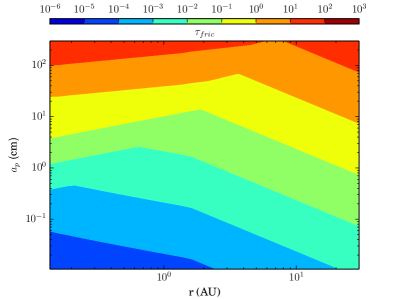
Figure 4.— Dimensionless friction timescale, $\tau_{\rm fric}$, map of pebbles in our fiducial disk model ($\dot{m}=10^{-9}\>M_{\odot}\>{\rm yr}^{-1}$, $\alpha=10^{-4}$).

Table 1Pebble Supply Reservoir Radii and Drift Timescales for Vulcan Planets

disk model	$M_{p,1}$	$r_{\rm 1200K}$	$r_{\rm res,1}$ (AU)	$t_{\rm drift}$ (no growth)	$t_{\rm drift}$ (w/ sweep-up growth)
($\dot{m}_{-9},\alpha$)	($M_{\oplus}$)	(AU)	($\epsilon_{p,1}=1,0.5,0.25$)	($10^{4}\>$yr, $\epsilon_{p,1}=1,0.5,0.25$)	($10^{4}\>$yr, $\epsilon_{p,1}=1,0.5,0.25$)
$0.1,10^{-4}$	0.96	0.060	3.35, 6.87, 14.3	6.20, 7.23, 8.18	0.748, 1.17, 1.71
$0.1,10^{-3}$	1.59	0.036	19.1, 40.2, 84.5	0.994, 1.22, 1.94	0.474, 0.697, 1.41
$1,10^{-4}$	3.43	0.167	1.75, 2.95, 5.45	16.3, 24.6, 33.6	0.798, 1.35, 2.35
$1,10^{-3}$	5.73	0.100	6.67, 13.7, 28.5	5.43, 6.37, 7.23	1.14, 1.67, 2.28
$10,10^{-4}$	12.3	0.464	1.93, 2.90, 4.47	17.7, 29.9, 50.4	0.671, 1.14, 2.08
$10,10^{-3}$	20.6	0.278	3.73, 6.14, 11.1	12.6, 19.8, 27.7	1.39, 2.40, 3.98

Note. — $t_{\rm drift}$ is evaluated for pebbles of initial radius of 1 mm, with the trajectory followed from $r_{\rm res,1}$ to the DZIB where $r=r_{1200\rm K}$ (for $\phi_{\rm DZIB}=0.76$).

The pebble evolution model of Hu et al. (2014) involves “sweep-up growth” of pebbles by accretion of small dust grains (we add pebble-pebble coagulation in the next section). Similar models have been proposed by Safronov (1972) and also been discussed by Dullemond & Dominik (2005) in the context of dust growth during vertical settling. Windmark et al. (2012) considered such a model as a mechanism by which cm-sized “seeds” can overcome the bouncing/fragmentation barrier to form planetesimals by sweeping up smaller grains.

Like Hu et al. (2014), we assume a pebble sweeps up all the dust within its geometric cross section if it is in the Epstein drag regime, where pebble size is comparable to a gas molecule’s mean free path. However, when a pebble enters the Stokes regime, the gas behaves more like a continuous fluid, forming a pressure wake in front of the pebble. We thus assume sweep up growth stops, as small dust grains are deflected by this pressure wake and flow away following gas streamlines.

To implement this model, in each time step $\delta t$, the mass growth of a pebble is:

$$\delta m_{p} = \pi a_{p}^{2}v_{\rm rel}\rho_{d}\delta t.$$ (23)

Here $\rho_{d}$ is mass of dust per unit volume in the disk, i.e., 1% of the gas density, $\rho$, for our fiducial initial conditions. $v_{\rm rel}$ is the relative velocity between a pebble and its surrounding gas, which is given by:

$$v_{\rm rel}=\left(1+\tau_{\rm fric}^{2}/4\right)^{1/2}v_{\rm r,p}.$$ (24)

We now calculate example trajectories of pebbles of initial radius of 1 mm that start at a radius in the disk equal to that of the pebble supply reservoir for a Vulcan planet, $r_{\rm res,1}$ (see Figure 5). The trajectories are shown for the cases with and without sweep-up growth, i.e., the latter being for pebbles of constant radius of 1 mm. These calculations are done for six different disk models, i.e., $\dot{m}_{-9}=0.1,1,10$ and $\alpha=10^{-4},10^{-3}$. In each disk, three different starting radii for $\epsilon_{p,1}=1,0.5,0.25$ are considered. These properties and the total drift times, $t_{\rm drift}$, for all these cases are listed in Table 1.

Figure 5 and Table 1 illustrate several points. First, note the dependence of Vulcan planet masses, $M_{p,1}$, and the pebble supply reservoir outer radii, $r_{\rm res,1}$, on disk properties. These planet masses range from about $1\>M_{\oplus}$ in the case of a low accretion rate, low viscosity disk, to about $20\>M_{\oplus}$ in a disk with a $100\times$ higher accretion rate and $10\times$ higher viscosity. Since disk mass surface densities are lower for higher viscosity disks, the corresponding reservoir radii also become larger in such cases. Thus $r_{\rm res,1}$ varies from just 1.75 AU (actually occurring in the fiducial case if $\epsilon_{p,1}=1$) to almost 100 AU in the low $\dot{m}$, high $\alpha$, low $\epsilon_{p,1}$ model.

Then the drift times from these radii to the location of planet formation, i.e., $r_{\rm 1200K}$, depend on whether the pebble is allowed to grow by sweep-up growth of small dust grains. Without growth, in the $\alpha=10^{-4}$ disks, we see that $t_{\rm drift}\gtrsim 10^{5}\>$yr. It takes longer to drift inwards in the high $\dot{m}$ disks, even though starting closer in, because the pebbles are in different drag regimes leading to different drag frictional timescales (eq. 21). This pattern is mirrored in the higher $\alpha$ disks, where we see that the no growth drift times can be as short as $\sim 10^{4}\>$yr even from $\sim$100 AU. Allowing pebbles to grow results in shorter drift timescales, since the pebbles approach sizes that lead to maximal drag force, i.e., minimal frictional timescales, leading to efficient radial migration, which then further enhances pebble growth. We notice that in all the six disk models considered the values of $t_{\rm drift}$ with sweep-up growth are quite similar, i.e., $\sim 10^{4}\>$yr. The pebbles can grow to sizes $\sim 1$ to 10 cm.

Thus we conclude that for a wide range of disk parameters ($\dot{m}\in[10^{-10},10^{-8}]\>M_{\odot}\>{\rm yr}^{-1}$, $\alpha\in[10^{-4},10^{-3}]$), the radial drift time scale is one or two orders of magnitude shorter than $t_{\rm form}$, based on an estimate of a steady-state supply rate of pebbles. This reflects the extreme limit of the pebble supply rate being boosted above the accretion limited rate because of the net radial drift of pebbles with respect to gas. It also assumes that the pebbles starting from within $r_{\rm res,1}$ will be able to sweep up a large fraction of the total solid mass, i.e., of dust, in this inner disk region. To advance beyond these simple estimates, we need to construct a global model of pebble evolution and supply in the disk.

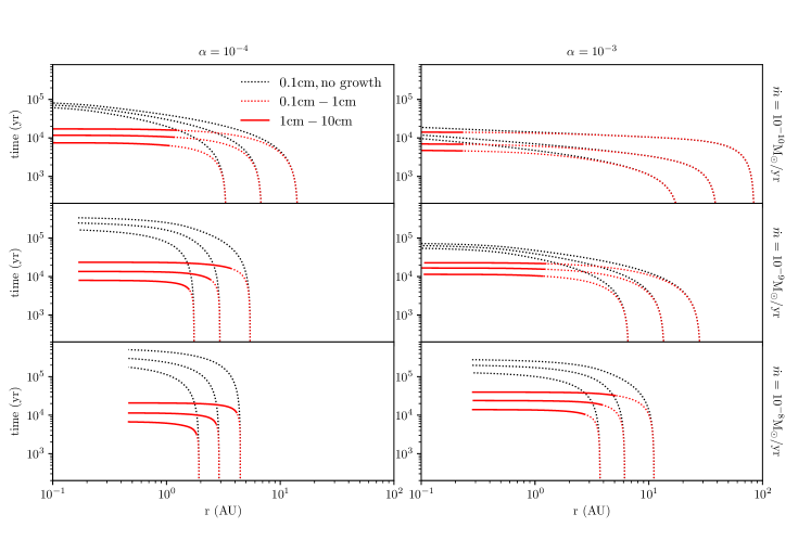
Figure 5.— Radial trajectories in time of pebbles with initial radii of 0.1 cm, starting from various supply reservoir outer boundaries for Vulcan planets with $\epsilon_{p}=1,0.5,0.25$ (see Table 1). The black dotted lines show models with no growth of the pebbles, i.e., they keep a constant radius of 0.1 cm. The red lines show models with growth via Stokes-limited sweep-up of small dust grains. Different styles of red lines represent different ranges of pebble sizes during this growth: dashed lines cover the size range of 0.1 to 1cm; solid lines cover 1 to 10 cm. Left column shows disks with $\alpha=10^{-4}$; right column with $\alpha=10^{-3}$. Top, middle and bottom rows show models with $\dot{m}=10^{-10},10^{-9},10^{-8}\>M_{\odot}\>{\rm yr}^{-1}$, respectively. Pebble trajectories are followed until an inner radius is reached where $r=r_{1200\rm K}$, $\phi_{\rm DZIB}=0.76$, expected to be the location of the DZIB.

5. Global Pebble Evolution Model

5.1. Numerical Implementation

Here we describe the basic algorithm used in an Eulerian pebble evolution model, including radial drift and growth (sweep-up plus coagulation). We sample a discrete grid in radial distance ($r$) and pebble radius ($a_{p}$). At any given radius, the model is intended to approximate conditions applicable to pebbles drifting inwards near the disk midplane.

We divide solids in the disk into two groups: larger particles treated as pebbles; smaller particles treated as dust. Dust represents particles smaller than a certain size threshold, for which we adopt $a_{p,{\rm min}}=0.01$ cm (as a fiducial choice), while pebbles are particles divided in different size bins. During radial drift, pebbles can grow by sweeping up dust (i.e., the Stokes-limited sweep-up growth model described in the previous section) and by coagulation with other pebbles.

The basic numerical approach in an “Eulerian” model is to find the fraction of material that is transported between neighboring cells within each time step. Considering pebble evolution, this fraction at radial grid cell $i$ and pebble size grid cell $j$, $f_{p}(i,j)$ is calculated as the sum of the radial drift fraction in $r$ space, $f_{p,r}(i,j)$ and size ($a_{p}$) space $f_{p,a}(i,j)$. The radial drift fraction of mass moved to the next radial grid, i.e., the mass fraction of pebble size $j$ at radial grid $i$, $f_{p,r}(i,j)$ is the ratio between radial drift distance to radial width of the ring shaped grid:

$$f_{p,r}(i,j) = v_{r,\rm i,j}\Delta t/\Delta r_{\rm ring},$$ (25)

where $\Delta r_{\rm ring}$ is the width of each radial grid, $\Delta t$ is time step, and $v_{r,\rm i,j}$ is radial drift velocity of pebble size $j$ at the center of the grid. This “center of box” first order approximation works because the variation of disk properties within each grid is very minor, especially with a logarithmic radial grid set up.

The size evolution of pebbles is more complicated. The difference between largest and smallest pebbles within one size bin becomes larger due to the nature of sweep up growth. At size bin $j$, the minimum size is denoted as $a_{\rm p,i,jmin}$, and the maximum is $a_{\rm p,i,jmax}$. Within one time step, a pebble with size $a_{\rm p,i,jmin}$ can grow to size $a_{\rm p,i,jmin}^{\prime}$, by sweeping up dust of mass $\delta m$ from eq. 23:

$$a_{\rm p,i,jmin}^{\prime}=\left(a_{\rm p,i,jmin}^{3}+\frac{3\delta m}{4\pi}\right)^{1/3}.$$ (26)

Similarly, a $a_{\rm p,i,jmax}$ sized pebble can grow to $a_{\rm p,i,jmax}^{\prime}$. Between size $a_{\rm p,i,j}$ and $a_{\rm p,i,j+1}$, there exists a size $a_{\rm p,i,jmid}$, that can grow to $a_{\rm p,i,jmax}$ in this time step, $\Delta t$. The value of $a_{\rm p,i,jmid}$ is obtained from linear interpolation of $a_{\rm p,i,jmin}$ and $a_{\rm p,i,jmax}$. Thus, pebbles below size $a_{\rm p,i,jmid}$ will stay in current size bin, while pebbles above $a_{\rm p,i,jmid}$ move to next size bin. With the assumption that pebble mass is distributed evenly within each size bin, we obtain the fractional mass in size space that grows to the next size bin:

$$f_{p,a}(i,j) = \frac{\left(a_{\rm p,i,jmax}-a_{\rm p,i,jmid}\right)}{\left(a_{\rm p,i,jmax}-a_{\rm p,i,jmin}\right)}.$$ (27)

To make the code more efficient, at each mesh in $r$ space, the time step is self adjustable, depending on the drift rate and growth rate of pebbles. The whole disk shares a larger time step for synchronization, while each mesh has its own sub time step that is a simple fraction ($1/n$) of the larger step. To achieve this, virtual rings are implemented between each mesh, recording fluxes from the outer mesh and supplying to inner meshes in each sub step.

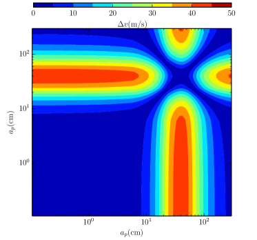
Figure 6.— Example of total disk plane relative velocities between different pebbles due to radial and cylindrical drift in the fiducial disk model ($\dot{m}_{-9}=1$, $\alpha=10^{-4}$) at 1 AU. These relative velocities are used in the pebble-pebble coagulation model.

A simple pebble-pebble interaction algorithm is also implemented. Here we ignore effects like Brownian motion, disk turbulence or vertical settling, so that only radial and cylindrical drift are considered for setting interaction velocities. When pebble size group $j$ meets group $k$, the number of two body interactions leading to coagulation, $N_{c}$, per unit area per time step, $\Delta t$, is calculated as (see Birnstiel et al., 2010):

$$N_{c}=S_{j,k}\Delta v_{j,k}\Delta tp_{c}N_{j}N_{k}/\sqrt{2\pi(h^{2}_{j}+h^{2}_{k})},$$ (28)

where $S_{j,k}=\pi(a_{p,j}+a_{p,k})^{2}$ is the coagulation cross section, $\Delta v_{j,k}$ is the relative velocity between pebble group j and group k, $N_{j}$ and $N_{k}$ are surface number densities of pebbles in these groups, $h_{j}$ and $h_{k}$ are pebble vertical scale heights, calculated as $h_{j}=h/\sqrt{1+\tau_{\rm fric,j}/\alpha}$, and $p_{c}$ is the coagulation efficiency given by:

$$p_{c}=\begin{cases}1,&\text{if}\ \Delta v\leq 10{\rm m/s}\\ 3-(\Delta v/5\>\rm m/s),&\text{if}\ 10{\rm m/s}<\Delta v\leq 15{\rm m/s}\\ 0,&\text{if}\ \Delta v\geq 15{\rm m/s}.\end{cases}$$ (29)

Thus when the relative speed is $>15$ m/s, there is a “fragmentation barrier” that prevents further pebble growth.

Figure 6 shows an example of the relative velocities occurring between different size groups at an 1 AU location in the fiducial disk with $\dot{m}=10^{-9}\>M_{\odot}\>{\rm yr}^{-1}$ and $\alpha=10^{-4}$. These range up to $\sim$40 m/s for pebbles with $a_{p}\sim 40\>$cm, but, for typical sizes of $\sim 1$ to 10 cm, are $\lesssim 10\>$m/s.

The final step of modeling coagulation is that of redistributing the masses of the coagulation products. Each pebble group has a certain range of sizes (i.e., masses), and the width of this range would be enlarged by coagulation, as the product’s minimum size is set by the combination of the smallest pebbles from both groups and the maximum size by combination of the largest pebbles. So the coagulated mass will be distributed into size bins ranging from $(a_{\rm p,i,jmin}^{3}+a_{\rm p,i,kmin}^{3})^{1/3}$ to $(a_{\rm p,i,jmax}^{3}+a_{\rm p,i,kmax}^{3})^{1/3}$.

The coagulation time step also follows a sub-step algorithm, in each mesh, with the condition that $\Delta t$ is chosen so that the fraction of pebbles (by number or mass) that coagulate is no larger than 0.02.

For our simulation domain, we only consider pebble evolution in the region outward of the pressure maximum of the DZIB, i.e., from about 0.1 AU to 30 AU.

The outer boundary of 30 AU is chosen as a representative outer disk scale, which contains a large enough dust reservoir to form a system of planets for the various disk models considered. However, this choice is somewhat arbitrary and, as we will see, we will mainly focus on the results of models that involve a steady injection of small pebbles at this outer boundary, so the initial reservoir of solid material is not particularly important.

The radial spatial resolutions of the model is set by 160 logarithmic divided grids, from 0.1 AU to 30 AU. We follow pebbles from a minimum particle radius of $a_{p,{\rm min}}$, while solids below this limit are considered to be “dust.” While $a_{p,{\rm min}}=0.01$ cm is the fiducial choice, we also consider models with $a_{p,{\rm min}}=0.1$ cm to explore the dependence of our results on this choice. Note, we use logarithmically spaced grids in pebble size space: $a_{p,j}=a_{p,{\rm min}}\times 10^{j\times 0.05}$. At the start of simulation, the dust mass surface density $\Sigma_{d}$ is set to be 1% of the gas mass surface density, $\Sigma_{g}$. The initial pebbles are given a mass surface density of $\Sigma_{p}$ that is 1% of $\Sigma_{d}$ (in the fiducial case; variation of this parameter is also explored). The distribution of the radii of the initial/injected pebbles are set to range from $a_{p,{\rm min}}$ to 0.3 cm with a number density versus size distribution following the equilibrium distribution of Birnstiel et al. (2015):

$${\rm d}n_{p}(a_{p})\propto a_{p}^{-5/8}{\rm d}a_{p}.$$ (30)

At the outer boundary, the disk is supplied with dust and pebbles given the steady state accretion rate and our adopted value of $f_{s}=0.01$, and the fiducial pebble to dust mass ratio is again 1% for the injected solids.

5.2. Fiducial Model Results & Effects of Accretion Rate, Initial Pebble Distribution, & Minimum Pebble Size

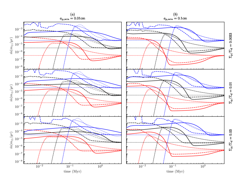
Figure 7.— (a) Left: Pebble accretion rate to the inner disk ($r=0.1\>$AU) region versus time for models with minimum pebble radius $a_{p,{\rm min}}=0.01\>$cm. The upper, middle and lower panels show different initial pebble to dust ratios $\Sigma_{p}/\Sigma_{d}=0.0033,0.01,0.03$, respectively, and the same values are also used for the injected pebble to dust ratios. Note that all models assume a constant solids (dust $+$ pebbles) to gas ratio of 0.01. In each panel, 3 different accretion rates are color coded. The solid black line shows the model of pebble evolution with only sweep-up growth for the case of the $\dot{m}=10^{-9}\>M_{\odot}\>{\rm yr}^{-1}$ disk with $\alpha=10^{-4}$. The dashed black line shows the equivalent result for the model that also includes pebble-pebble coagulation. The horizontal black dotted line shows the steady state pebble accretion rate if all solids are in the form of pebbles. Equivalent results for higher ($\dot{m}=10^{-8}\>M_{\odot}\>{\rm yr}^{-1}$, blue) and lower $(\dot{m}=10^{-10}\>M_{\odot}\>{\rm yr}^{-1}$, red) accretion rate disks are shown. The lines in lighter color shading show results of disks that are initially empty of pebbles, i.e., pebbles only appear via injection at the outer boundary at 30 AU. Note the pebble accretion rates in the simulated disks can be larger than the steady state rates because of the sweep-up and delivery of the initial dust reservoir in the disk, but the asymptotic behavior at late times is towards this steady state rate. (b) Right : As (a) but now for $a_{p,{\rm min}}=0.1\>$cm.

We first present results in Figure 7 for the time evolution of the mass flux of pebbles delivered to the inner disk inner boundary ($r=0.1\>{\rm AU}$) for disks with viscosity parameter $\alpha=10^{-4}$. Our fiducial case adops a minimum pebble radius of $a_{p,{\rm min}}=0.01\>$cm (left column panels of Figure 7), but we also show the results for $a_{p,{\rm min}}=0.1\>$cm (right column). Our fiducial choice of initial and injected pebble to dust mass surface densities is $\Sigma_{p}/\Sigma_{d}=0.01$ (middle row), but we also show the results for ratios that are three times smaller (top row) and larger (bottom row). Our fiducial case has a steady accretion rate of $\dot{m}=10^{-9}\>M_{\odot}\>{\rm yr}^{-1}$ (black/grey lines), but we explore results of varying this from $10^{-10}\>M_{\odot}\>{\rm yr}^{-1}$ (red lines) to $10^{-8}\>M_{\odot}\>{\rm yr}^{-1}$ (blue lines). We show the results of the case of pebble evolution where only sweep-up growth of dust is considered (solid lines), and then also for the case where pebble-pebble coagulation is included (dashed lines). Finally, our fiducial model involves the initial disk from 0.1 to 30 AU being populated with pebbles with the given ratio of $\Sigma_{p}/\Sigma_{d}$ (dark lines), however we also consider the case of an initially “empty” disk, i.e., no pebbles, only dust, with pebbles only appearing via injection at 30 AU (lighter shaded lines). The steady-state pebble supply rates assuming all solids are in pebbles are shown by the horizontal dotted lines in the panels, i.e., three lines for the three accretion rates of $10^{-10},10^{-9},10^{-8}\>M_{\odot}\>{\rm yr}^{-1}$.

Considering the fiducial case in the left-middle panel, we see there is an initial period of pebble supply rates that are greater than the steady state rate due to delivery of solid material (mostly dust) that was initialized to be present in the disk, i.e., from 0.1 to 30 AU. Pebble-pebble coagulation leads to more efficient sweep-up of this material so that the period of elevated supply rate is shorter, but more intense. The late-time behavior of the models is asymptotic approach to the steady state supply rate (from above).

This trend is basically repeated in the higher $\dot{m}$ case. However, in the lower $\dot{m}$ case we see that the pebble supply rate drops below the expected steady state rate, and then slowly approaches it from below. Figure 7b shows the same models, but now for $a_{p,{\rm min}}=0.1\>$cm, which has the effect of initializing with and continuing to inject with a smaller number of larger pebbles. Similar behavior is seen, with an initial “spike” phase of elevated pebble supple rates, which are shorter, but more intense, if pebble-pebble coagulation is modeled. Now, however, the $\dot{m}=10^{-9}\>M_{\odot}\>{\rm yr}^{-1}$ case also exhibits a pebble supply rate that falls below the steady state supply rate immediately after the spike phase.

The above behavior can be better understood, by comparing to the same results in lighter colored lines that show the models in which there are no initial pebbles in the disk: they only appear via injection at the 30 AU boundary. These models show initial elevated pebble supply rates due to delivery of the initial dust from the disk, but do not show the decremented phases where pebble accretion rate is below the steady state rate.

We conclude that the initial spike phase, due to delivery of initial disk dust, is a somewhat artificial feature of our model, dependent on the initial conditions. A subsequent decremented supply rate phase can occur in some cases if there has been very efficient sweep-up of the initial dust by an initial population of pebbles and there is a relatively long period of time needed for the injected pebbles to drift in to the inner disk. The limiting case of no initial pebbles in the disk is instructive in that it tells us the time needed for the disk to reach a quasi equilibrium state where pebble supply rate at the inner boundary equals that injected at 30 AU. For only sweep-up growth, this timescale can be $\gtrsim 1\>$Myr for the high accretion rate case, and somewhat shorter for lower $\dot{m}$ cases. However, including pebble-pebble coagulation reduces these timescales. Since early high accretion rate phases are expected to last $\lesssim 1\>$Myr, i.e., the evolution from the protostellar disk phase, this tells us that a globally self-consistent model may need to take into account the evolving disk structure due to a declining accretion rate and that a steady state may not be reached in certain circumstances.

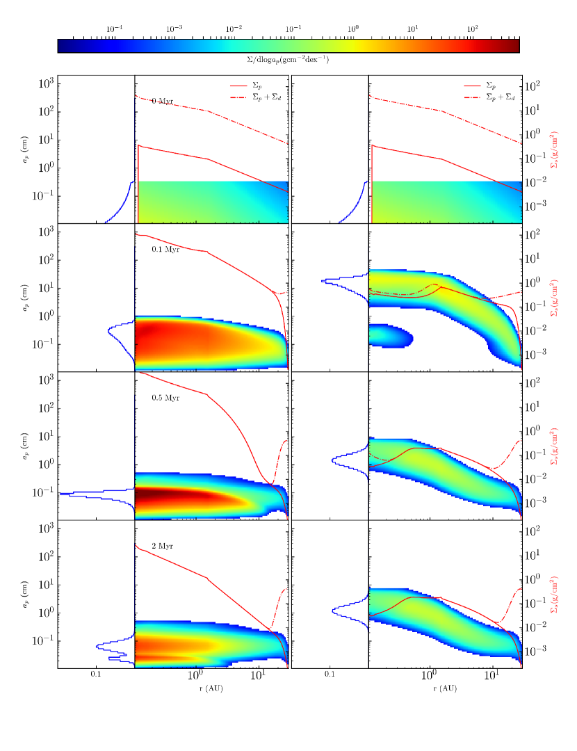
Figure 8.— Evolution of pebble size versus orbital radius distributions from the initial condition (top row), to 0.1 Myr (2nd row), to 0.5 Myr (3rd row) to 2 Myr (bottom row). The left column shows the sweep-up only growth model. The right column shows the sweep-up plus pebble-pebble coagulation growth model. In each panel the color scale shows the distribution of the pebbles, while on the left there is a projected histogram of the sizes of those pebble inside 1 AU radii. The red solid line shows the mass surface density of pebbles. The red dot-dashed line shows the total mass surface density of solids (dust plus pebbles). When these overlap, most of the solid mass is in pebbles, which is achieved by late times in both models.

Figure 8 shows the radial profiles of the dust size distributions for our fiducial model with and without pebble-pebble coagulation. The size distribution of pebbles delivered to the inner disk is significantly larger in the latter case. The figure also shows the radial profiles of the mass surface densities of pebbles and total solids, which allows assessment of the mass fraction of solids that is in pebbles compared to dust (recall that our modeling is of the midplane region).

In models with pebble coagulation, the sweeping up of dust is not as efficient in the inner disk as in the sweep-up only model. As seen from Figure 8, the pebble mass surface density is significantly lower than the total solids mass surface density, while in the sweep-up only model, pebbles dominate the total solid mass starting even at 0.1 Myr. The growth rate of pebble coagulation scales with the square of pebble number density $N_{p}^{2}$, while sweep up growth scales with $N_{p}$. During the early stages in the inner disk, where the pebble density is high, fast mutual coagulation produces large, Stokes-limited pebbles without sweeping up much dust. The inner disk can maintain a high dust fraction until the pebble flux from the outer disk arrives.

Another feature worth noticing in the coagulation model is the transient behavior at 0.1 Myr. The pebbles are divided into two groups in the inner disk. There are two contributing factors: the Stokes-limited sweep-up growth forbids the further sweep-up growth of some initial pebbles in the inner disk; and the 15 m/s coagulation speed limit stops them being coagulated into larger sizes, while their mutual coagulations are very inefficient due to small cross sections and low relative velocities (see Figure 6).

5.3. Effects of $\alpha$ Viscosity

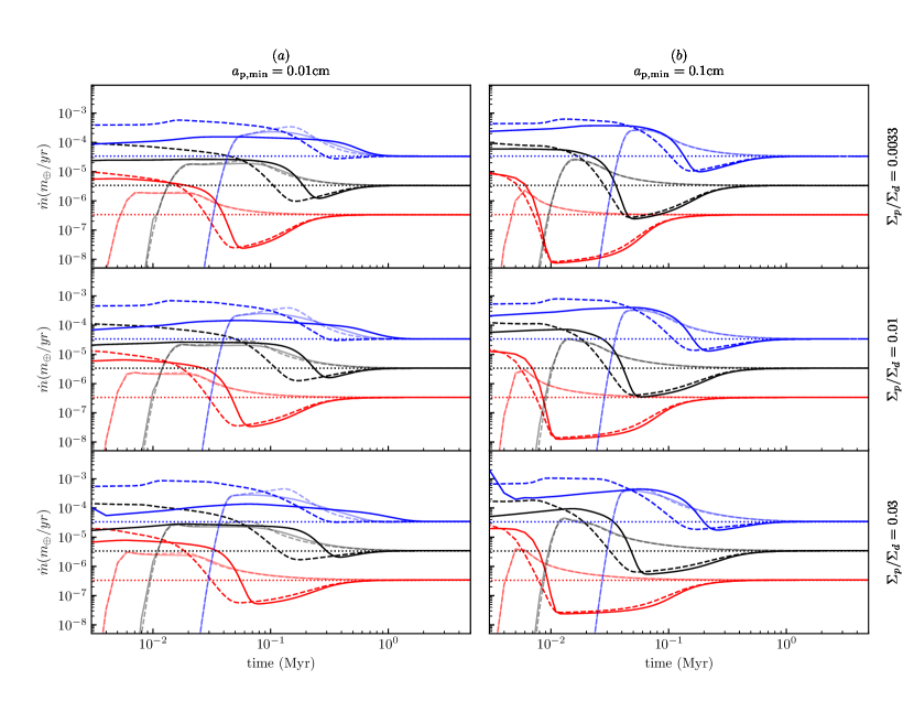
Figure 9.— (a) Left: As Figure 7a, but now for disks with $\alpha=10^{-3}$.(b) Right: As (a) but now for $a_{p,{\rm min}}=0.1\>$cm.

The appropriate value of the effective viscosity, parameterized via $\alpha$, is very uncertain. Here we repeat the analysis of the previous sub-section, but now for disks with $\alpha=10^{-3}$. These results are shown in Figure 9. In our modeling, variation of $\alpha$ plays a similar role as $\dot{m}$, as it mainly affects mass surface density, i.e., $\Sigma_{g}\propto\alpha^{-4/5}$ (see eq. 2). Higher $\alpha$ disks thus have a smaller initial dust reservoir, i.e., in the scale of the 30 AU disk, and less efficient sweep-up growth. Thus, note that the pebble flux profile in a disk of $\dot{m}=10^{-9}\>M_{\odot}\>{\rm yr}^{-1},\alpha=10^{-3}$ is quite similar to the one with $\dot{m}=10^{-10}\>M_{\odot}\>{\rm yr}^{-1},\alpha=10^{-4}$. Though the dust in the inner disk transfers mostly into pebbles, as in the low $\alpha$ case, the solids in the outer disk stay mostly in the form of dust for a much longer time. This effect is visible in Figure 10, which shows the radial dependence of the pebble size distributions and the relative levels of $\Sigma_{p}$ and $(\Sigma_{p}+\Sigma_{d})$ for the higher $\alpha$ disks.

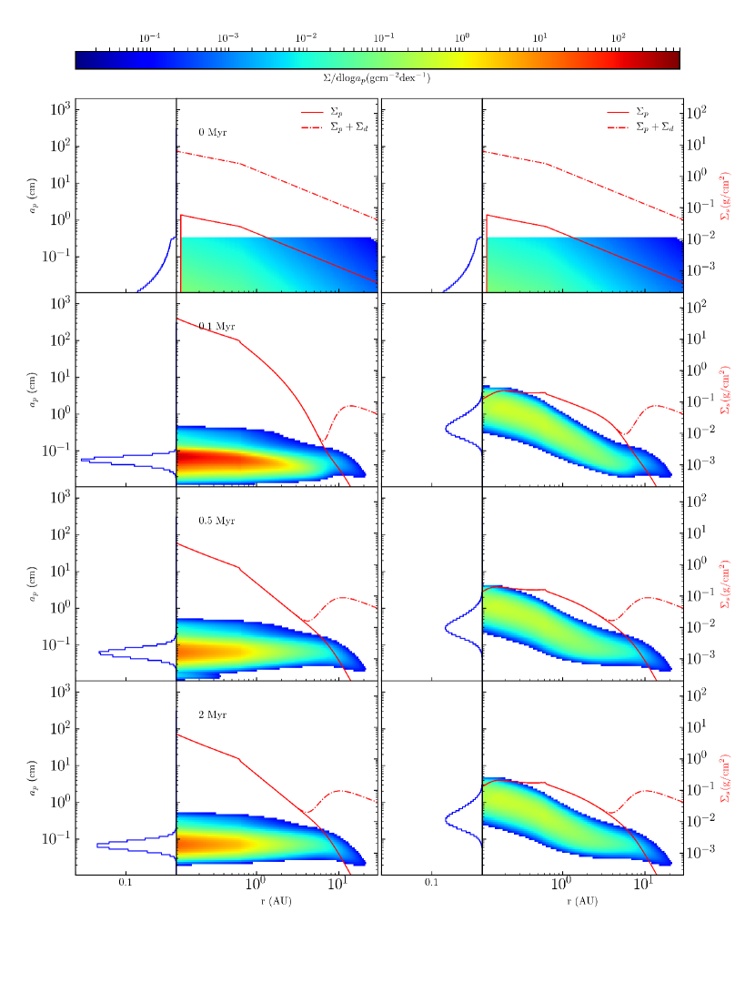
Figure 10.— Same as Figure 8, but showing disk with viscosity parameter $\alpha=10^{-3}$. The major difference is in the outer disk: significantly more solids remain in the form of dust than in the disk with $\alpha=10^{-4}$, thus resulting in a lower pebble flux after the dust in the inner disk has been swept-up.

6. Assembling a STIP

6.1. Steady Accretion Rate Disks

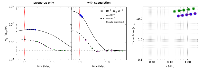
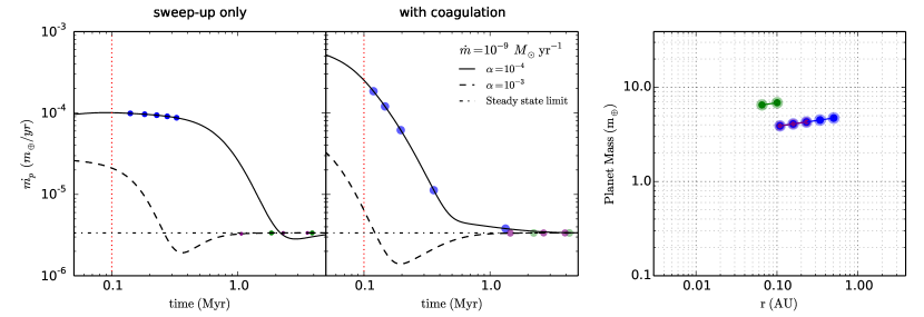
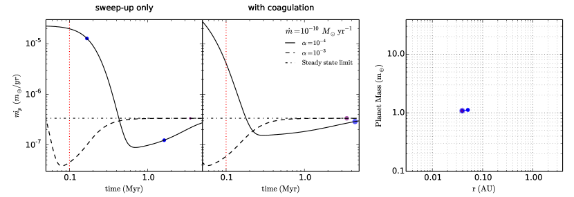
Figure 11.— (a) Top row: Example of STIP formation history (left and middle panels) and orbital architecture, i.e., planet mass versus orbital radius (right panel), given a pebble supply rate history for a model with $a_{p,{\rm min}}=0.01\>$cm and a steady gas accretion rate of $\dot{m}=10^{-8}\>M_{\odot}\>{\rm yr}^{-1}$. The results of models with only sweep-up growth of pebbles are shown in the left panel. The black solid line shows the pebble supply rate to the inner disk with $\alpha=10^{-4}$, and black dashed line shows pebble supply rate with $\alpha=10^{-3}$. The dot-dashed line marks the steady state pebble flux limit. The colored dots on the pebble delivery lines indicate the formation time of each planet, with blue dots for $\alpha=10^{-4}$, green dots for $\alpha=10^{-3}$, and purple dots for global disk $\alpha=10^{-3}$ but with calculation of $M_{G,D}$ done for $\alpha=10^{-4}$, i.e., a lower value of $\alpha$ near the DZIB. Note that in these models planet formation is assumed to start at 0.1 Myr (marked by the vertical dashed line). The middle panel shows the equivalent results, but now including pebble-pebble coagulation. (b) Middle row: As (a) but for disk accretion rates of $\dot{m}=10^{-9}M_{\odot}\>{\rm yr}^{-1}$. (c) Bottom row: As (a) but for disk accretion rates of $\dot{m}=10^{-10}M_{\odot}\>{\rm yr}^{-1}$. The disks with lower accretion rates can fail to form all five planets within the 5 Myr period considered.

We now consider the implications of these models for the timescale of assembling an entire STIP. As a specific example, we will consider the ability of disk models to form a five-planet system and the time it takes them to do so. We compare the accumulated mass from the delivered inner disk pebble flux to the required mass of the planets, i.e., set by the gap opening condition for $M_{\rm G,D}$ from eq. 3.2.

A noticeable feature of our modeled pebble flux is the “spike” phase at the beginning of the simulations, which can transport a large amount of solids ($\sim 50M_{\oplus}$) in less than 0.5 Myr. However, this spike feature mostly reflects the adopted initial condition of pebbles and dust in the inner ($\lesssim 10\>$AU) disk. Since these solids in reality could have already drifted in at an earlier phase of the disk’s evolution, here we ignore the pebbles delivered in the early spike phase up to 0.1 Myr. Still, we will see that our results do depend on how the initial conditions of the disks are set-up.

In the context of IOPF, building a STIP starts with the innermost “Vulcan” planet at $r_{\rm 1200K}$. After that, here, for simplicity, we assume that the orbit of each subsequent planet is 20 Hill radii away from the previously formed planet, which is close to the median value from observations (Paper I) and within the range of DZIB retreat distances modeled in Paper III as being due to increased ionization via penetration of protostellar X-rays. The planet mass is calculated as $M_{\rm G,D,1.44}$ using eq. 3.2. We simply assume all accumulated mass of pebbles will be transferred into planets, i.e., the radially drifting pebbles will be caught by the DZIB pressure trap and later accreted with 100% efficiency by the protoplanet.

The results of this modeling for our fiducial disk ($\dot{m}=10^{-9}\>M_{\odot}\>{\rm yr^{-1}},\alpha=1\times 10^{-4}$) are shown with solid lines in the left pair of panels in the middle row of Figure 11. Here, the first planet starts forming 0.1 Myr after the spike phase, and the fifth has completed formation within the following 0.4 Myr in the case of sweep-up only pebble evolution and within 1.5 Myr in the case including pebble-pebble coagulation (blue dots mark the time of formation of each planet). The difference is due the different pebble supply rates, with the first model more heavily influenced by the initial spike phase from the initial dust reservoir. The orbital distribution and masses of the planets are shown in the rightmost panel of the middle row (again shown as blue dots).

Equivalent models with $\alpha=1\times 10^{-3}$ tend to have lower pebble supply rates (dashed lines). If this value of $\alpha$ also holds in the DZIB region, then the gap opening mass is increased, implying more massive planets. In this case only two such planets (green dots) have time to form within 5 Myr.

The top and bottom rows of Figure 11 show equivalent results for $\dot{m}=10^{-8}\>M_{\odot}\>{\rm yr^{-1}}$ and $\dot{m}=10^{-10}\>M_{\odot}\>{\rm yr^{-1}}$, respectively. Higher/lower accretion rates imply higher/lower gap-opening masses, but with a sub-linear scaling. The total mass of pebbles delivered to the inner region in a given time scales more steeply with accretion rate. Thus, it becomes more difficult for lower accretion rate disk models to be able to form the entire five planet system. Overall, when comparing models with different $\dot{m}$ and $\alpha$, we find that to form a realistic STIP, the disk should have $\dot{m}\sim 10^{-9}M_{\odot}\>{\rm yr}^{-1}$ and viscous $\alpha$ no more than $\sim 2\times 10^{-4}$.

6.2. Evolving Disks

Lifetimes of protoplanetary disks are estimated to range from $\sim$1 to 10 Myrs (e.g., Alexander et al., 2014; Espaillat et al., 2014). The effects of an evolving disk have been previously considered in dust evolution models. For example, Birnstiel et al. (2010) set up a disk model subject to viscous evolution and gravitational instability, starting from the very early infall phase. It gives a relatively constant accretion rate starting from 0.15 Myr to 1 Myr. Other methods involve adopting simple functional forms for the evolution of the accretion rate, such a power law or exponential decay (e.g., Hueso & Guillot, 2005; Bitsch et al., 2015). The disk modeled by Bitsch et al. (2015) has an accretion rate that evolves as:

$$\dot{m}=\dot{m}_{0}e^{-t/t_{0}},$$ (31)

with $\dot{m}_{0}=7.24\times 10^{-9}\>M_{\odot}\>{\rm yr^{-1}}$ and $t_{0}=3.1\times 10^{5}\>$yr. We adopt the same functional form, but with $\dot{m}_{0}=1.0\times 10^{-9}\>M_{\odot}\>{\rm yr^{-1}}$ and $t_{0}=4.34\times 10^{5}\>$yr, so that the accretion rate declines by a factor of 10 in 1 Myr.

In our numerical modeling, we update the disk properties, i.e., the accretion rate, every 1000 years. Note, in such models of exponentially declining accretion rate, the disk evolution is not fully self consistent for its accretion history, i.e., the declining $\Sigma_{g}$ does not match the viscous radial drift of gas. Thus these models should be viewed as being simple “toy” models of disk evolution. Note also, when we force the gas disk properties to evolve with an exponentially declining rate, we have a choice about how we treat the associated dust that may be mixed together with the gas. We consider two extreme cases: Case A: the dust content of the disk, i.e., $\Sigma_{d}$, does not evolve with the declining gas, i.e., it would remain at a steady mass surface density, except for the effects of radial drift (due to the assumed $\alpha$ viscosity) and sweep-up by pebbles; Case B, the dust content of the disk, i.e., $\Sigma_{d}$, is decreased with the same exponential decay rate of the gas, with this decay factor applied multiplicatively on top of any other changes due to radial drift and sweep-up by pebbles.

In principle, there are now several parameters that may be varied in these models: $\dot{m}_{0}$, $t_{0}$, $t_{\rm IOPF}$ (i.e., the time when the first planet starts to form), in addition to other model parameters already introduced, such as $\alpha$ and $a_{p,{\rm min}}$. Furthermore, there are the choices of: Case A or B, introduced above; whether or not pebble-pebble coagulation is included in the modeling; and whether or not the disk model is initially “empty” of pebbles. It is not our intention here to carry out a full exploration of the parameter space of all these models. Rather, here we present several example models of representative cases, in particularly focussing on the examples of parameter combinations that produce realistic STIPs within reasonable timescales.

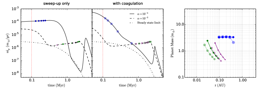
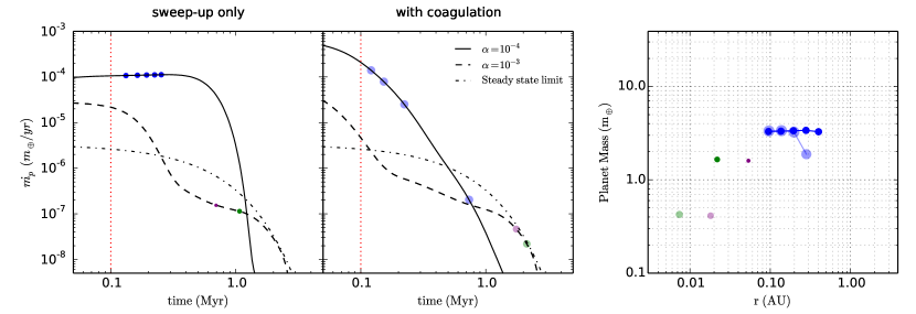
Figure 12.— (a) Top row: Example of STIP formation history (left and middle panel) and orbital architecture (right panel) in an evolving disk (treated as Case A, see text), using same color coding and styles as Figure 11. Here, planet formation also starts at $t_{\rm IOPF}=0.1\>$Myr. The only addition is the lighter shaded points in the right panel represent planets formed in the “with coagulation” model. (b) Bottom row: As (a), but now for Case B, i.e., dust content of disk is also scaled with the exponential decay function.

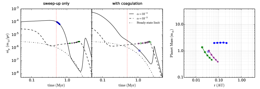
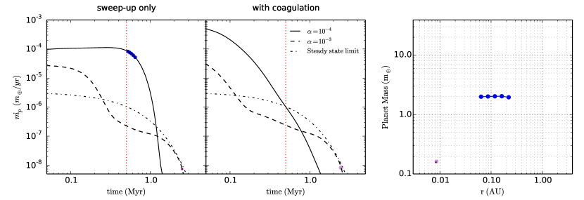
Figure 13.— (a) Top row: Same as Figure 12a, i.e., Case A models, but now with planet formation starting at $t_{\rm IOPF}=0.5\>$Myr. (b) Bottom row: As (a), but now for Case B, i.e., dust content of disk is also scaled with the exponential decay function.

Following the format of Figure 11, Figure 12 now shows example models with $\dot{m}_{0}=10^{-9}\>M_{\odot}\>{\rm yr}^{-1}$, $t_{0}=4.34\times 10^{5}\>$yr, $t_{\rm IOPF}=0.1\>$Myr and $a_{p,{\rm min}}=0.01\>$cm. Case A is shown in the top row; Case B in the bottom row. In each row, models with low $\alpha$ ($10^{-4}$), high $\alpha$ ($10^{-3}$) and “mixed” $\alpha$ (i.e., $10^{-4}$ in the DZIB region; $10^{-3}$ in the main disk region beyond the DZIB region that is relevant for pebble growth and supply) for the cases without and with pebble-pebble coagulation. In these models, the value of $\alpha$ in the DZIB region has a direct effect on the mass of the planets needed to open up a gap, i.e., lower mass planets in lower viscosity disks. The value of $\alpha$ in the main disk region beyond the DZIB affects global disk structure in the zone responsible for pebble growth and supply: in particular, lower viscosity implies a higher disk mass, for a given accretion rate, and so a more massive reservoir of dust for planet formation. The “mixed” $\alpha$ model that is presented is a simple means of allowing for there being different values of viscosity in DZIB that affect planet masses and in the main disk region that affect pebble growth and supply.

Compared to the steady disk models with $\dot{m}=10^{-9}\>M_{\odot}\>{\rm yr}^{-1}$, these evolving disk models have lower late-time pebble delivery rates. Planets forming at these later times have lower masses, since the gap opening mass is lower for lower accretion rates. We see that certain combinations of models lead to planet formation being spread out in time over a few Myr, which leads to a significant decline in planet mass with orbital radius. This is not a particular feature of observed STIPs, modulo uncertainties in inferring their masses from observed sizes (see, e.g., Paper I, II). To obtain relatively flat distributions of planet masses versus orbital radii requires IOPF to be mostly complete within $\sim t_{0}$ (and thus for $t_{\rm IOPF}\ll t_{0}$). Only the low $\alpha$ models achieve these conditions.

The influence of the spike phase of enhanced pebble supply rate at early times can extend the time period when reasonable STIPs can be formed by IOPF, especially in the sweep-up only pebble evolution models. This is also illustrated in Figure 13, which shows the same results as in Figure 12, but now for $t_{\rm IOPF}=0.5\>$Myr. Only in the low $\alpha$, sweep-up only models does a STIP with flat mass versus orbital radius distribution form.

We note that the flux increase after about 2.5 Myr in Case A is a result of both leftover dust from early phase and the relatively large Stokes numbers of the injected pebbles at late stages. The injected pebbles, i.e., with radii of 0.01 cm to 0.3 cm, have relatively small Stokes numbers in the early phases, when gas densities are higher. However, the Stokes number increases significantly as $\dot{m}$ drops. Still, in the models considered here, this late-time pulse of delivered pebbles is not significant compared to the early pebble delivery that formed the STIP.

Note these are systems with modest initial accretion rates: $\dot{m}=10^{-9}M_{\odot}\>{\rm yr^{-1}}$. If IOPF starts at even higher $\dot{m}$, then the planets formed would be significantly more massive than typical observed STIPs (unless the DZIB $\alpha$ is much smaller than values we have considered).

7. Discussion and Conclusions

In this paper we have presented improved models of Inside-Out Planet Formation (IOPF), with a particular focus on understanding if most solids will be delivered to the inner disk in the form of pebbles (i.e., the raw materials for planet formation) and then the implied formation times and constraints on disk properties during the time of IOPF. The models presented here are an attempt at calculating “IOPF population synthesis”, and can be compared to other such models based on other theoretical frameworks (e.g., Ida & Lin, 2004; Bitsch et al., 2015).

We first constructed improved disk models, extending to 30 AU, especially using realistic opacities and including the effect of the active disk to passive disk transition. Next, we expanded on the work of Paper III to examine the gap opening condition (i.e., pressure maximum displacement from the planet) over a wider range of viscosities (especially extending to the low $\alpha$ regime that seems to be needed for IOPF) and accretion rates. We find that the Duffell (2015) analytic description of the gap opening criterion is a better description of the results than the simple viscous criterion we used previously in Papers I to III. This implies that planets are more massive in the low $\alpha$ regime, i.e., still $\sim 4\>M_{\oplus}$ for $\alpha=10^{-4}$ for $\dot{m}=10^{-9}\>M_{\odot}\>{\rm yr}^{-1}$.

Next we examined pebble evolution in these disks, presenting models for how a single pebble is expected to evolve via Stokes-limited sweep-up of dust and pebble-pebble coagulation. This formed the basis of a global pebble evolution model, i.e., of a population of pebbles, for given choices of initial conditions and boundary conditions (i.e., the injected pebbles at 30 AU).

Simple constraints on timescales of first, “Vulcan” planet formation were derived with the single pebble evolution model, under the assumption of a given efficiency of solids being incorporated into pebbles (Table 1). Fiducial estimates based on drift times from the reservoir radius are $\sim 10^{5}\>$yr to form the first planet. The global pebble evolution models showed that large, near unity fractions of solids are expected to be incorporated into pebbles (with the caveat that our disk models apply to the midplane layer conditions; but this is where most solids are expected to have settled). By the time they reach the inner AU, pebble sizes are typically $\sim 0.1\>$cm in the sweep-up only models and about a few cm in the models including pebble-pebble coagulation. Such predictions are potentially testable by observations of protoplanetary disks (e.g., Pérez et al., 2012; Trotta et al., 2013; Testi et al., 2014; Tazzari et al., 2016).

We utilized the global pebble evolution models in disks with steady accretion rates to predict pebble delivery rates to the inner disk. We showed the effects of model assumptions, including whether the disk is initially populated with pebbles. The models show an initial “spike” phase of an elevated pebble flux compared to the steady state rate due to sweeping up of the initial dust reservoir, which decays away in about a Myr.

Finally we used these models to predict the formation history of STIPs forming via IOPF. Formation locations of the Vulcan planets were set self-consistently at $r_{\rm 1200K}$ and with masses that depend on accretion rate, location, and disk viscosity. The timescale to form a five-planet system was assessed, with an overall cap of 5 Myr imposed. In steady accretion rate disks, these models showed a preference for $\dot{m}\sim 10^{-9}\>M_{\odot}\>{\rm yr}^{-1}$. Higher accretion rate models form planets that are too massive and too far away from the star. Lower accretion rate models do not have high enough pebble delivery rates to form several planets. Extending to evolving disk models introduces additional parameters and model choices. For simple evolving disk models treated with an exponentially declining accretion rate, we require IOPF to be completed within this decay time $\sim 1\>$Myr in order to preserve the observed relatively flat scaling of planet mass with orbital radius.

We note that IOPF’s apparent preference for accretion rates of $\dot{m}\sim 10^{-9}\>M_{\odot}\>{\rm yr}^{-1}$ is quite consistent with observed accretion rates of young stellar objects, including transition disk systems (e.g., Williams & Cieza, 2011; Manara et al., 2014, 2016). At even lower accretion rates, the rate of photoevaporation of the disk may become comparable, potentially terminating or greatly reducing the supply of gas to the inner disk (e.g., Ercolano et al., 2009; Owen et al., 2012; Ercolano et al., 2014). However, if the solids are mostly settled to the disk midplane in the form of pebbles, as indicated by the results of our global pebble evolution models, then their supply is less likely to be affected by photoevaporation. Nevertheless a more complete global evolution model of IOPF, planned for a future study, should also account for additional processes such as photoevaporation to examine its effects on gas supply to the inner disk region. Self-consistent constraints of disk lifetimes that are predicted by either residual core infall and/or photoevaporation will also need to be considered in this modeling.

References

- Alexander et al. (2014) Alexander, R., Pascucci, I., Andrews, S., Armitage, P., & Cieza, L. 2014, Protostars and Planets VI, 475
- Armitage (2007) Armitage, P. J. 2007, arXiv:astro-ph/0701485
- Baruteau et al. (2014) Baruteau, C., Crida, A., Paardekooper, S. J. et al. 2014, Protostars and Planets VI, Univ. Arizona Press, Tucson, p.667
- Birnstiel et al. (2010) Birnstiel, T., Dullemond, C. P., & Brauer, F. 2010, A&A, 513, A79
- Birnstiel et al. (2012) Birnstiel, T., Klahr, H., & Ercolano, B. 2012, A&A, 539, A148
- Birnstiel et al. (2015) Birnstiel, T., Andrews, S. M., Pinilla, P., & Kama, M. 2015, ApJ, 813, L14
- Bitsch et al. (2015) Bitsch, B., Lambrechts, M., & Johansen, A. 2015, A&A, 582A.112B
- Bitsch et al. (2018) Bitsch, B., Morbidelli, A., Johansen, A., et al. 2018, arXiv:1801.02341
- Brauer et al. (2008) Brauer, F., Dullemond, C. P., & Henning, T. 2008, A&A, 480, 859
- Chatterjee & Ford (2015) Chatterjee, S., & Ford, E. B. 2015, ApJ, 803, 33C
- Chatterjee & Tan (2014) Chatterjee, S., & Tan, J. C. 2014, ApJ, 780, 53
- Chatterjee & Tan (2015) Chatterjee, S., & Tan, J. C. 2015, ApJ, 798, L32
- Chiang & Laughlin (2013) Chiang, E., & Laughlin, G. 2013, MNRAS, 431, 3444
- Chiang & Goldreich (1997) Chiang, E. I., & Goldreich, P. 1997, ApJ, 490, 368
- Cossou et al. (2013) Cossou, C., Raymond, S. N. & Pierens, A. 2013, A&A, 553L, 2C
- Cossou et al. (2014) Cossou, C., Raymond, S. N. & Pierens, A. 2014, IAUS, 299, 360C
- Dullemond & Dominik (2005) Dullemond, C. P., & Dominik, C. 2005, A&A, 434, 971
- Duffell & MacFadyen (2013) Duffell, P. C., & MacFadyen, A. I. 2013, ApJ, 769, 41
- Duffell (2015) Duffell, P. C. 2015, ApJ, 807, L11
- Dumusque et al. (2014) Dumusque, X., Bonomo, A. S., Haywood, R. D., et al. 2014, ApJ, 789, 154
- Dzyurkevich et al. (2010) Dzyurkevich, N., Flock, M., Turner, N. J., Klahr, H., & Henning, T. 2010, A&A, 515, A70
- Ercolano et al. (2009) Ercolano B., Clarke C. J., Drake J. J., 2009, ApJ, 699, 1639
- Ercolano et al. (2014) Ercolano, B., Mayr, D., Owen, J. E., Rosotti, G., & Manara, C. F. 2014, MNRAS, 439, 256
- Espaillat et al. (2014) Espaillat, C., Muzerolle, J., Najita, J., et al. 2014, Protostars and Planets VI, 497
- Fabrycky et al. (2014) Fabrycky, D. C., Lissauer, J. J., Ragozzine, D. et al. 2014, ApJ, 790, 146
- Fang & Margot (2012) Fang, J. & Margot, J. L. 2012, ApJ, 761, 92
- Fung et al. (2014) Fung, J., Shi, J.-M., & Chiang, E. 2014, ApJ, 782, 88
- Goldreich & Schlichting (2014) Goldreich, P. & Schlichting, H. E. 2014, AJ, 147, 32G
- Hansen & Murray (2013) Hansen, B. & Murray, N. 2013, ApJ, 775, 53
- Hansen & Murray (2012) Hansen, B. & Murray, N. 2012, ApJ, 751, 158
- Hu et al. (2014) Hu, X., Tan, J. C., & Chatterjee, S. 2014, IAU Symp., 310, 66
- Hu et al. (2016) Hu, X., Zhu, Z., Tan, J. C., & Chatterjee, S. 2016, ApJ, 816, 19
- Hueso & Guillot (2005) Hueso, R., & Guillot, T. 2005, A&A, 442, 703
- Ida & Lin (2004) Ida, S., & Lin, D. N. C. 2004, ApJ, 604, 388
- Izidoro et al. (2017) Izidoro, A., Ogihara, M., Raymond, S. N., et al. 2017, MNRAS, 470, 1750
- Kley & Nelson (2012) Kley, W. & Nelson, R. P. 2012, ARA&A, 50, 211
- Krijt et al. (2016) Krijt, S., Ormel, C. W., Dominik, C., & Tielens, A. G. G. M. 2016, A&A, 586, A20
- Lambrechts et al. (2014) Lambrechts, M. & Johansen, A. and Morbidelli, A. 2014, A&A, 572A, 35L
- Lin & Papaloizou (1993) Lin, D. N. C., & Papaloizou, J. C. B. 1993, Protostars and Planets III, Univ. Arizona Press, Tucson, p. 749
- Liu et al. (2017) Liu, B., Ormel, C. W., & Lin, D. N. C. 2017, A&A, 601, A15
- Manara et al. (2014) Manara, C. F., Testi, L., Natta, A. et al. 2014, A&A, 568, A18
- Manara et al. (2016) Manara, C. F., Rosotti, G., Testi, L., Natta, A. et al. 2016, A&A, 591, L3
- van der Marel et al. (2016) van der Marel, N., Verhaar, B. W., van Terwisga, S., et al. 2016, A&A, 592, A126
- Masset (2000) Masset, F. S. 2000, A&A, 141,165
- McNeil & Nelson (2010) McNeil, D. S. & Nelson, R. P. 2010, MNRAS, 401, 1691
- Mohanty et al. (2013) Mohanty, S., Ercolano, B., & Turner, N. J. 2013, ApJ, 764, 65
- Mullally et al. (2015) Mullally, F., Coughlin, J. L., Thompson, S. E. et al. 2015, ApJS, 217, 31M
- Ogihara et al. (2015) Ogihara, M., Morbidelli, A. & Guillot, T. 2015, A&A, 578A, 36O
- Owen et al. (2012) Owen J. E., Clarke C. J., & Ercolano B., 2012, MNRAS, 422, 1880
- Pérez et al. (2012) Pérez, L. M., Carpenter, J. M., Chandler, C. J., et al. 2012, ApJ, 760, L17
- Raymond & Cossou (2014) Raymond, S. N. & Cossou, C. 2014, MNRAS, 440L, 11R
- Ribas et al. (2015) Ribas, Á., Bouy, H., & Merín, B. 2015, A&A, 576, A52
- Safronov (1972) Safronov, V. S. 1972, Evolution of the protoplanetary cloud and formation of the earth and planets (Jerusalem: Keter Publishing House)
- Sato et al. (2015) Sato, T., Okuzumi, S., & Ida, S. 2015, arXiv:1512.02414
- Schlichting (2014) Schlichting, H. E. 2014, ApJ, 795L, 15S
- Shakura & Sunyaev (1973) Shakura, N. I., & Sunyaev, R. A. 1973, A&A, 24, 337
- Tazzari et al. (2016) Tazzari, M., Testi, L., Ercolano, B., et al. 2016, A&A, 588, A53
- Testi et al. (2014) Testi, L., Birnstiel, T., Ricci, L., et al. 2014, Protostars and Planets VI, 339
- Toomre (1964) Toomre, A. 1964, ApJ, 139, 1217T
- Trotta et al. (2013) Trotta, F., Testi, L., Natta, A., Isella, A., & Ricci, L. 2013, A&A, 558, A64
- Varnière & Tagger (2006) Varnière, P. and Tagger, M. 2006, A&A, 446L, 13V
- Williams & Cieza (2011) Williams, J. P., & Cieza, L. A. 2011, ARA&A, 49, 67
- Windmark et al. (2012) Windmark, F., Birnstiel, T., Güttler, C., et al. 2012, A&A, 540, A73
- Youdin & Goodman (2005) Youdin, A. N. & Goodman, J. 2005, ApJ, 620, 459Y
- Zhu et al. (2009) Zhu, Z., Hartmann, L., & Gammie, C. 2009, ApJ, 694, 1045
- Zhu et al. (2012) Zhu, Z., Nelson, R. P., Dong, R., Espaillat, C., & Hartmann, L. 2012, ApJ, 755, 6
- Zhu et al. (2013) Zhu, Z., Stone, J. M., & Rafikov, R. R. 2013, ApJ, 768, 143