Bright X-ray flares from Sgr A*

Abstract

We address a question whether the observed light curves of X-ray flares originating deep in galactic cores can give us independent constraints on the mass of the central supermassive black hole. To this end we study four brightest flares that have been recorded from Sagittarius A*. They all exhibit an asymmetric shape consistent with a combination of two intrinsically separate peaks that occur at a certain time-delay with respect to each other, and are characterized by their mutual flux ratio and the profile of raising/declining parts. Such asymmetric shapes arise naturally in the scenario of a temporary flash from a source orbiting near a supermassive black hole, at radius of only $\sim 10$–$20$ gravitational radii. An interplay of relativistic effects is responsible for the modulation of the observed light curves: Doppler boosting, gravitational redshift, light focusing, and light-travel time delays. We find the flare properties to be in agreement with the simulations (our ray-tracing code sim5lib). The inferred mass for each of the flares comes out in agreement with previous estimates based on orbits of stars; the latter have been observed at radii and over time-scales two orders of magnitude larger than those typical for the X-ray flares, so the two methods are genuinely different. We test the reliability of the method by applying it to another object, namely, the Seyfert I galaxy RE J1034+396.

1 Introduction

The radio source Sagittarius A* (Sgr A*) at the dynamical center of our galaxy (Balick & Brown, 1974) shows variability in all wavelengths visible to us (e.g. Brown & Lo, 1982; Macquart et al., 2006; Eckart et al., 2004; Eckart et al., 2006; Eckart et al., 2008; Hornstein et al., 2007; Yusef-Zadeh et al., 2006, 2009; Dodds-Eden et al., 2009). Sgr A* is usually visible at sub-mm and radio frequencies, while detectable flares at near infrared (NIR) wavelengths can be observed about 2-6 times per day (Genzel et al., 2003; Ghez et al., 2004; Yusef-Zadeh et al., 2006; Nishiyama et al., 2009). The biggest excursions have been observed at X-ray frequencies, although flares at near-infrared frequencies occur more often: X-ray flares about 10 time brighter than the quiescent background flux occur about once per day (Baganoff et al., 2001). The first observation of an X-ray flare of Sgr A* was reported by Baganoff et al. (2001) and shows a peculiar asymmetry, it consists of two distinct peaks and a drop in between. The authors attribute the emission to accretion processes near the super-massive black hole (SMBH) (for a recent review on the validity of that assumption see Eckart et al., 2017). Porquet et al. (2003) published an observation of an even brighter flare, also with an asymmetric shape consisting of two peaks. Another bright flare was observed by Porquet et al. (2008), together with some less luminous ones, which will not be discussed further in this treatise. The bright flare however, shows again an asymmetrical shape. One of the latest very bright X-ray flare was published by Nowak et al. (2012) and it also exhibits an asymmetric shape, which is modeled by the authors as two Gaussians. Here, only these four brightest X-ray flares will be analyzed, since it is not feasible to make accurate statements about less bright flares, due to their limited signal to noise ratio.

Hotspot models (Stella & Vietri, 1998, 1999) have been tested as a mechanism to explain the flares of Sgr A* by numerous authors, mainly applied to near infrared observations (Genzel et al., 2003; Broderick & Loeb, 2005, 2006; Meyer et al., 2006b; Meyer et al., 2006a, 2007; Trippe et al., 2007; Dexter & Agol, 2009; Zamaninasab et al., 2010, 2011) to look for quasi periodic oscillations (QPO) appearing as substructures of some NIR-flares that were observed from Sgr A*. Eckart et al. (2004) reported the first simultaneous observations of a particular Sgr A* flare at near infrared as well as X-ray wavelengths. This suggests that NIR and X-ray flares of Sgr A* have the same origin and result from the same physical process. Mossoux et al. (2015) have applied a hotspot model to an X-ray flare of Sgr A*, but find that this scenario is not sufficient to model this particular flare.

In the following we will use the term ’hotspot’ or blob if we refer to relativistic orbital motion of a luminous matter component around the supermassive black hole as the prime reason for the observed phenomena. Here, we argue that the this scenario is a good model for Sgr A*’s X-ray variability. Furthermore, this scenario makes it possible to constrain the mass of the central black hole. There have already been a number of different attempts to constrain the mass which must be located at the position of Sgr A*. Wollman et al. (1977) applied a virial analysis to the radial velocities of ionized gas and determined a mass of $(2-4)\times 10^{6}M_{\odot}$. However, gas is not just influenced by gravity, and so measurements of the velocity dispersion of stars is a better estimate for the mass which is, however, in agreement with those resulting from gas motions (Rieke & Rieke, 1988; McGinn et al., 1989; Sellgren et al., 1990; Haller et al., 1996). Due to the large radius of this method, within which the mass must be enclosed, it is not possible to infer the existence of a black hole from these measurements alone. Employing the use of virial estimators and estimators of Bahcall & Tremaine (1981), Genzel et al. (1996) arrived at a central mass of $3\times 10^{6}M_{\odot}$, surrounded by a star cluster with a mass of $10^{6}M_{\odot}$. Eckart et al. (2002) showed for the first time that S-cluster star S2 is on a bound orbit around SgrA*. Improved orbital elements of S2 were given shortly after by Schödel et al. (2002) and Ghez et al. (2003). Using Kepler’s third law, the enclosed mass can be estimated, if the distance to the Galactic center can be accurately determined. Gillessen et al. (2009) analyzed the orbits of several stars of the S-cluster and found an enclosed mass of $4.3\times 10^{6}M_{\odot}$. The latest measurements of Sgr A*’s mass and its distance to us employed multiple stellar orbits and were published by Boehle et al. (2016). The authors find a mass estimate of $4.02\pm 0.16\pm 0.04\times 10^{6}M_{\odot}$ and their estimate on the distance is $7.86\pm 0.14\pm 0.04$ kpc. The two uncertainties correspond to the statistical and the systematic part of the uncertainties. Furthermore, their analysis results in a limit of $0.13\times 10^{6}M_{\odot}$ for the extended dark mass within $0.1$ pc at $99.7\%$ confidence. A first robust estimate of this limit of the extended mass contribution was derived by Mouawad et al. (2005).

In conclusion there is enough circumstantial evidence for the existence of a supermassive black hole at the position of Sgr A*. However, there have been no attempts to estimate the mass at scales of the order of a couple of gravitational radii. In the following we will outline a method using a relativistic model, which makes it possible to constrain the enclosed mass to within $25r_{g}$. If the method proves to be reliable, it is an appropriate way to test general relativity in the presence of the strong gravitational field of a supermassive black hole.

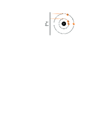
Figure 1: Illustration of the origin of the double-peak structure in the total flux. The blobs marked with an ’L’ are magnified by gravitational lensing, while they are behind the black hole from the observer’s point of view. That is, they are positioned on the focal line, along the orbital section $Q$ outlined by the dashed line. The blobs marked with a ’D’ are Doppler-boosted, because they are moving ’directly towards’ (in terms of geodesics) the observer, as indicated by the orange lines representing the geodesics from the source to the observer. The ’field of view’ is equivalent to the ’detector plane’ in which the object is imaged.

2 Description of the simulations

In this section we first give a brief summary of the simulations and then justify and describe the methodology we use to model the brightest observed X-ray flares. After summarizing essential facts on the radiation mechanism and characteristic features of the emission in different wave-bands, we describe the details of the ray-tracing code that is used and then discuss the setup of the model, which differs from the usual hotspot model.

2.1 Summary of the method

We fit the shapes of the brightest flares leaving the time-scale in periods measured in gravitational units of $t_{g}=GM/c^{3}$, hence, leaving the mass as a free parameter. Then the flare time-scale in periods is matched with the actual time length of the observed flare. This allows us to derive black hole mass distributions from the simulations. The median values and median errors of these non-Gaussian distributions then correspond to the expected black hole mass and its uncertainty. We apply the method to SgrA* and to the Seyfert I galaxy RE J1034+396.

2.2 Flares

The discussion of the radiation mechanism shows that the intrinsic flux density of the source component can be assumed to be rather constant during the rapid and strong modulations by relativistic effects like Doppler-boosting (beaming) or lensing. Based on discussions in Neilsen et al. (2015); Eckart et al. (2012); Yuan et al. (2004); Baganoff et al. (2001); Markoff et al. (2001) we conclude that the intrinsic flux density evolution of X-ray luminous components is dominated by the time-scales of the relevant sub-mm peaking synchrotron components. This then implies that rapid flux density variations in the X-ray domain are more likely a result of relativistic effects like boosting and lensing rather than synchrotron cooling due to high energetic electrons. This is supported by the fact that the times scales for the boosting and lensing events are very short (in the few minutes to 10 minute range - depending on the geometry) compared to those on which the underlying emission is varying. Also (again depending on the geometry) the amplification factors of these relativistic effects can easily be several 10. In addition, the flare lengths indicate that the flares themselves originate close to the black hole (Baganoff et al., 2001, 2003) making these relativistic modulations also frequent and relevant. This scenario justifies that we model the flare profiles with an orbiting spot model. This model is a generalized surrogate-model to characterize the behavior of (in this case) X-ray emitting matter in the gravitational field of a super massive black hole. Of course, we only consider the variable non-thermal part of the SgrA* emission. This source is embedded in an extended non-variable Bremsstrahlung component (Baganoff et al., 2001, 2003) and during times the source is not flaring, the non-thermal flux drops well below the Bremsstrahlung flux level. This constant component is therefore removed before we fit the flares. Restricting the modelling to the brightest flares, therefore essentially completely avoids the risk of overlapping flare events, such that we truly model only one flare at a time.

2.3 Ray-tracing code

We introduce a numerical code based on the Kerr-metric library sim5lib written in the programming language $C$. The code is also capable to describe polarization transport. However, unfortunately there is no polarization data available for the flares we investigate here. A future X-ray polarimeter might record an abundance of information that could help constrain the black hole’s parameters. In an upcoming paper these polarization simulations will be discussed further and applied to the near-infrared. However, here we restrict ourselves to the total flux of Sgr A* at X-ray wavelengths. The library sim5lib uses the mechanism outlined by Dexter & Agol (2009), so instead of using a set of pre-calculated transfer-functions on a grid of parameters and then interpolating, as is the case, i.e., for the Karas-Yaqoob (KY) code (Dovc̆iak, 2004; Meyer et al., 2006b; Meyer et al., 2006a; Zamaninasab et al., 2010, 2011), we use sim5lib to explicitly compute the null geodesics and then track the emission along them using a parallel transport. The null geodesics are obtained by numerically solving the equation governing photon motion in Kerr space-time. Starting at a maximum domain radius $R_{max}$, which is far enough away from the black hole so that any general relativistic effects from there to the observer are negligible, and going in the direction of the BH, we look for those geodesics which reach an emitting source and discard the rest. Once these relevant geodesics are found, the emission can be traced from the source back to the observer in Boyer-Lindquist coordinates. Although this method demands much more computing power than using pre-calculated transfer functions, it allows us to control all parameters of the geodesics while the general relativistic effects on the rays in the presence of a strong gravitational field are included intrinsically. This comprises changes of the emission angle, rotation of the polarization angle and gravitational lensing. During the passage of the hotspot behind the black hole, as viewed by the observer, the high gravity of the black hole leads to bending of the geodesics. This gravitational lensing effect is at its strongest on the focal line. This is demonstrated in Fig. 1. The fraction of the orbit between the boosting and lensing points varies with the radius of the orbit, owing to the stronger bending of the geodesics close to the black hole. In Fig. 1 this fraction is highlighted by a dashed line parallel to the corresponding orbit. The comparable figure (Fig.12) in Eckart et al. (2017) also shows the corresponding light curve with the boosting and lensing flux peaks labeled. For comparison see also the light curves, particularly in Fig. 2(b)

Table 1: Basic parameters of the simulations.

Parameter	Values	Description
$a$	0.5	BH spin
$M$	1	BH mass
$i$	5∘, 10∘, … , 90∘	inclination
$D_{0}$	0.5 $r_{g}$, 1 $r_{g}$, … , 5.0 $r_{g}$	size of the blob
$R_{0}$	6 $r_{g}$, 8 $r_{g}$, … , 24 $r_{g}$	blob’s radial position
$\phi_{0}$	90	starting azimuth angle
$n_{e}$	1	electron number density
$R_{max}$	40 $r_{g}$	max. domain radius
Nx	150	resolution in pixels
frames	100	time frames per orbit
step	0.1 $r_{g}$	step along geodesics

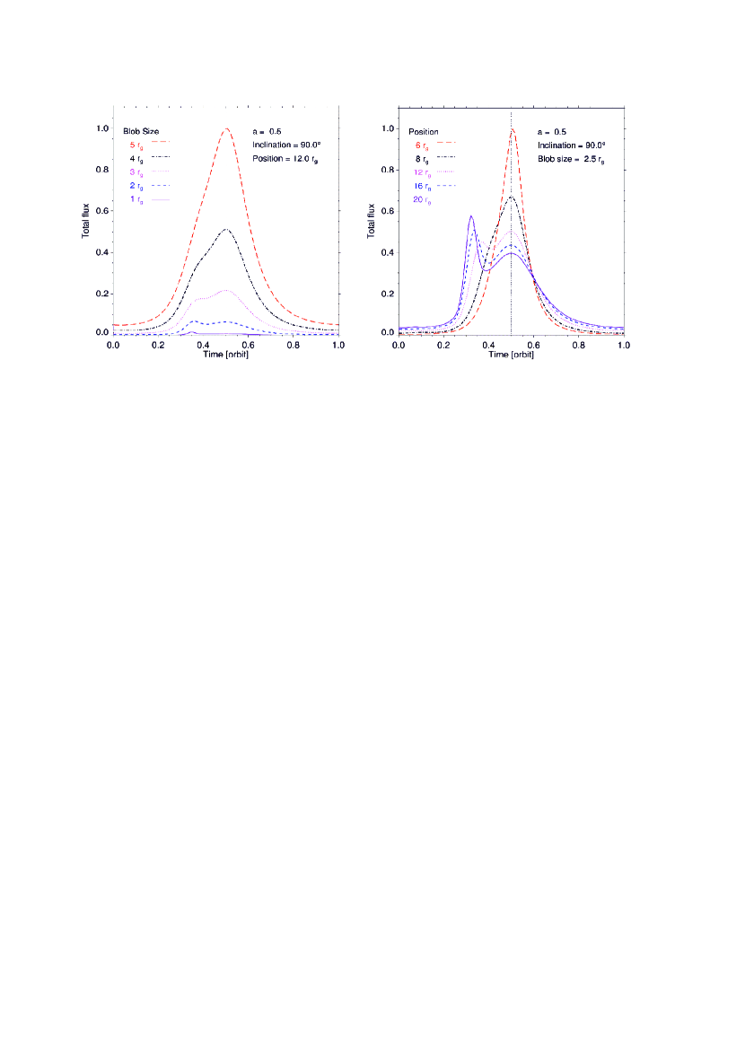
Figure 2: a) Left: Illustrates the influence of the blob’s size on the shape of the light curve. The blobs of different sizes (5 $r_{g}$ red long dashed, 4 $r_{g}$ black dash-dotted, 3 $r_{g}$ magenta dotted, 2 $r_{g}$ blue short dashed and 1 $r_{g}$ solid purple line) are orbiting at a radial position of 12 $r_{g}$ around a black hole with spin 0.5, the viewing angle is 90 ^∘ (edge on). The light curves are normalized to the maximum of the peak value of the light curve for the blob with the size 5 $r_{g}$ and shifted such that the Doppler-peak is at the center. b) Right: Illustrates the influence of the blob’s position on the shape of the light curve. The blobs are orbiting at different positions (6 $r_{g}$ red long dashed, 8 $r_{g}$ black dash-dotted, 12 $r_{g}$ magenta dotted, 16 $r_{g}$ blue short dashed and 20 $r_{g}$ solid purple line) and have a size of 2.5 $r_{g}$ around a black hole with spin 0.5, the viewing angle is 90 ^∘ (edge on). The light curves are normalized to the maximum of the peak value of the light curve for the blob with the size 5 $r_{g}$ and shifted such that the Doppler-peak is at the center.

Additionally, the special relativistic Doppler-boosting on the intensity of the radiation which is caused by aberration (Einstein, 1905) is taken into account as well. While the source moves away from the observer, the emission is reduced, whereas it is magnified for an approaching source. Finally, the strong gravitational field of the black hole presents a potential well, which exerts another redshift on the radiation. We take these two effects into account by introducing another factor, the g-factor (Dovc̆iak, 2004):

$$g=\frac{\nu_{0}}{\nu_{e}}=\frac{p_{0t}}{p_{i}U^{i}}=\frac{E_{\infty}}{p_{i}U^{i}},$$ (1)

where $\nu_{0}$ is the frequency of the observed photons, $\nu_{e}$ the frequency of the emitted photons, $p_{0t}$ the time component of the four-momentum of the photon as measured by an observer at infinity, and $U^{i}$ the four-velocity of the hotspot.

2.4 Setup of the models

Usually the hotspot scenario is employed to model a localized brightness excess within an accretion flow. A hotspot could arise through magnetic turbulence in a magneto-hydrodynamic accretion flow (Balbus & Hawley, 1991; Armitage & Reynolds, 2003), vortices and flux tubes (Abramowicz et al., 1992), magnetic flares (Poutanen & Fabian, 1999; Życki, 2002), interactions of stars with an accretion disk (Dai et al., 2010), or magnetic reconnection (Yuan et al., 2009). According to Eckart et al. (2012) it is most likely that the X-ray flares of Sgr A* (see also Eckart et al., 2002; Baganoff et al., 2001). are caused by a synchrotron self-Compton process. However, in this paper we only model the light curves resulting from the hotspot (or ’blob’) motion and not the physical mechanism that leads to the emission. The idea is that instead of an accretion disk, there are several clumps of matter of different sizes on different orbits with changing radii and viewing angles. These blobs of matter could have a similar origin as in the scenario of Jalali et al. (2014), only on a much smaller scale. A cloud could be compressed by the black hole’s strong gravity and then quickly disrupted. However, in the following only enhanced blob luminosity over half an orbit is needed. This is sufficient to distinguish between different relativistic effects. A cloud that is below the detection limit, could be magnified by the relativistic effects strongly enough such that it results in a flare, when viewed by the observer. The variability of Sgr A* would in this sense result from a physical one-state statistical process, as was argued by Witzel et al. (2014).

2.4.1 The modelling parameters

The important parameters that are varied in the simulations are the blob’s size $D_{0}$, the radial position of its orbit $R_{0}$ and the blob’s orbital inclination $i$ with respect to the observer. An overview of all the parameters of the model can be found in Table 1. Most of the other parameters are of lesser importance and - for the purpose of the fit done in periods and gravitational units $t_{g}$ - can be set to constant values as described below. This is the minimum set of parameters required to describe the motion of an emitting source in the gravitational field of a super massive black hole.

To model the hotspot we use a three dimensional Gaussian which emits uniformly in all directions, and is assumed to be in Keplerian motion in a stable orbit around a black hole.

$$K=n_{e}\,\mathrm{exp}\left[-\frac{1}{2}\frac{x^{i}x_{i}+\left(x^{i}U_{i}\right)^{2}}{D_{0}^{2}}\right],$$ (2)

where $n_{e}$ is the number density of electrons, $x_{i}$ the vector difference between the position of the photon and the center of the blob, $U_{i}$ the Keplerian four-velocity of the plasma and $D_{0}$ is a measure of the size of the blob, given in gravitational units. In our simulations we can safely assume $n_{e}$ to be 1, because in our model the number density is only a scaling factor for the luminosity.

Nothing is assumed about the mass of this black hole: all computations are undertaken in gravitational units. This will allow us to infer constraints on the black holes’ mass after the fitting process. Apart from determining the innermost stable circular orbit (ISCO) of the model, the spin of the black hole $a$ does not exert any noticeable influence on the shape of the light curves. Here, we only consider a black hole with prograde spin, that is $a\in[0,1)$, and in the orbiting hotspot model the spin is a variable of the period of the orbit ($G=c=1$):

$$P_{g}=2\pi[R^{3/2}+a]~{}~{}~{},$$ (3)

where $P_{g}$ is in geometrical units, and $R$ is the radius of the orbit, measured in units of the gravitational radius. Alternatively, we can write (Dovc̆iak, 2004):

$$P_{T}=310(R^{3/2}+a)M_{7}=49.3P_{g}\times M_{7}~{}~{}~{},$$ (4)

with $P_{T}$ in seconds and the mass $M$ in units of $10^{7}M_{\odot}$. Thus we choose $a=0.5$ and in doing so accept an uncertainty of $\pm\pi$ of the period. The lowest radius which is taken into account using $R=6r_{g}$, with $M=0.4\times M_{7}$, $a=0.5$ and $R=6r_{g}$, leads to a period $P_{T}\sim 31min$. From equation 4 we can see that the $\Delta a=0.5$ uncertainty of the spin results in a relative uncertainty of $\pm 3\%$ of the period.

In our simulations we consider various inclinations of the hotspot orbit (see Tab. 1 for the range) with respect to the spin axis of the black hole. The viewing angle is measured from the rotational axis of the black hole, so when we assume that the spin axis remains the same while we vary the viewing angle (i.e. the inclination of the orbit), another uncertainty is introduced owing to the precession due to the Lense-Thirring effect (Lense & Thirring, 1918). According to Merritt et al. (2010), the precession time-scale is given as

$$T=\frac{P}{4a}\bigg{[}\frac{c^{2}a_{sma}(1-e^{2})}{GM}\bigg{]}^{3/2},$$ (5)

where $P$ is the period in physical units, $a_{sma}$ the semi-major axis and $e$ the eccentricity of the orbit. Here, we are assuming a circular orbit, thus we have

$$T=\frac{P}{4a}\bigg{[}\frac{c^{2}R}{GM}\bigg{]}^{3/2},$$ (6)

or, with $G=c=1$ and $a=0.5$,

$$T=\frac{P}{2}R^{3/2}.$$ (7)

For the case of the smallest radius taken into account $R=6\times r_{g}$ this timescale is more than seven times that of the period of the orbit. For all radii which are bigger, it is even more than that. Thus, precession effects on the inclination can be neglected in our considerations, especially considering that the step width between inclinations is $5^{\circ}$.

3 The Simulations

The relativistic effects which are predominantly responsible for the magnification, gravitational lensing and the Doppler-boost, occur within within less than a fraction ($Q$) of an orbit. This matches well with the life time estimates of the orbiting spots (see Fig. 1). Theoretically, an accretion disk spot is assumed to rarely last for much longer than about one orbit (Schnittman, 2005; Schnittman et al., 2006; Meyer et al., 2006b; Adams & Watkins, 1995). In fact, a third of an orbital time-scale is sometimes indicated (e.g. see discussion in section 5.1.1. by Eckart et al., 2008; Schnittman et al., 2006). This time-scale is also well matched by our full width half maximum flare lengths of about 0.3 obits in Fig. 1. Depending on the distance of the hotspot from the black hole this then covers the observed overall flare time-scales very well and is also compatible with the time-scale for the intrinsic variation of the emission as discussed previously. Both constant (e.g. Fig.1 in Abramowicz et al., 1991) and exponentially decaying (Schnittman et al., 2006) light curves are assumes in the literature. Assuming an exponential decay of the spot flux density over the characteristic time-scale $t_{lifetime}\sim 0.3t_{orbit}$ then the drop will only be less than 50% over the section $Q$ and only 25% over the actual boosting and lensing phases. This result can be applied to SgrA* since all theoretical magneto-hydrodynamic accretion models show a so called ’central mid-plane’ which is comparable to a disk (Mościbrodzka et al., 2009; Mościbrodzka & Falcke, 2013; Mościbrodzka et al., 2014). We consider the hotspot as the dominant part of a much fainter disk component that we do not model. This also supports the choice of spots on circular orbits as a surrogate model for radiating matter close to the SMBH as highly elliptical orbits due to infalling matter are probably strongly suppressed. In a viscous environment with multiple gaseous clouds (as expected for ’central mid-planes’ resulting from magneto-hydrodynamic accretion models), clouds on crossing orbits can be excluded as their collisions are highly dissipative. As (semi-)stable trajectories in such an environment circular orbits are preferred.

Also, at least for SgrA* we do not claim repeated orbital periods mainly for the reasons above and due to the lack of observational evidences. However, the situation could be more complex as can be seen from the example J1034-396 that we refer to towards the end of the article. If the light curve of this source is interpreted using an orbiting spot model then multiple orbital periods and longer spot life times could be involved.

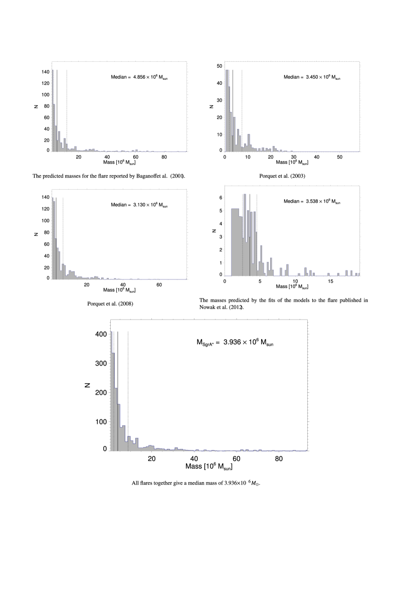
Figure 3: Weighted histograms of the predicted masses for all the models for the four flares taken into account.

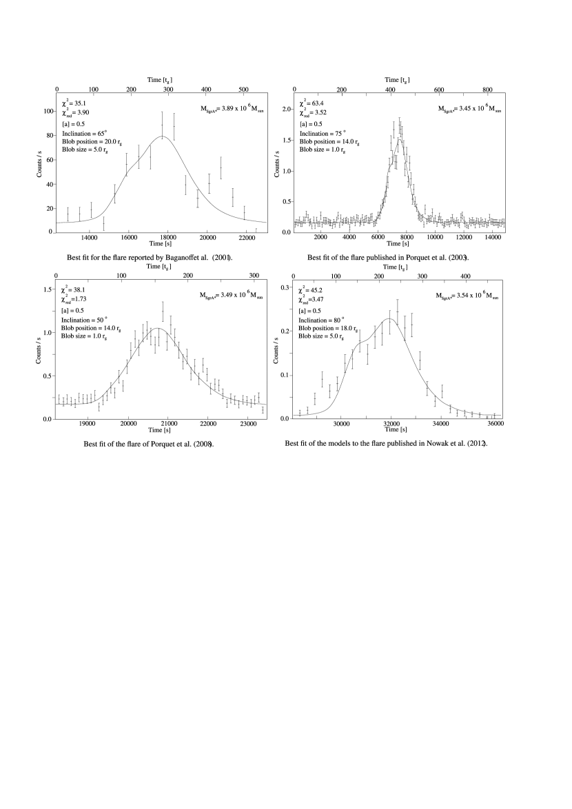
Figure 4: Best fits for the four analyzed flares in their respective median bin.

Broderick & Loeb (2006) find that the size of the hotspot indeed does not have a dominant influence on the light curves. However, as can be seen in Fig. 2ab, the simulations with sim5lib show a clear dependency of the shape of the flare on the size of the plasma blob, as well as on the distance of the blob to the black hole. In several previous ray-tracing simulations with a two-dimensional hotspot (e.g. Meyer et al., 2006b; Meyer et al., 2006a; Zamaninasab et al., 2010, 2011) this relation was not apparent. This is because high inclinations are needed in order to see this effect, which is problematic with a two-dimensional source. Mossoux et al. (2015) noted that the ratio between those two peaks is influenced by the blob’s size, which is confirmed by our simulations. We interpret this to arise because of the specifically different natures of the two relevant effects, which favor different conditions for the highest possible relative magnification. For a small emitting region (i.e. a blob size of $\sim 0.5~{}r_{g}$), the magnification due to lensing is much more effective than the magnification due to the Doppler-effect. A sufficiently large hotspot (i.e. a blob size of $\sim 5~{}r_{g}$) however, will magnify only slightly by virtue of the black hole’s gravitational lensing effect, in comparison to its much more efficient magnification via the Doppler-effect.

Furthermore, the radius of the orbit has a major influence on the profile of the light curves, as can be seen from Fig 2. In particular, the size of the hotspot itself is not the only factor which influences the ratio of the two peaks: the further a blob is away from the black hole, the bigger the blob needs to be in order to result in a dominant magnification of the Doppler-effect. While on the other hand, a blob close to the black hole requires a particularly small blob in order to yield a dominant gravitational lensing magnification.

An additional effect that influences the light curves’ shapes is dependent on the radial position as well. For blobs on a close orbit around a black hole, the geodesics are bent so much that the Doppler-peak immediately follows the lensing-peak, whereas for larger orbits the peaks can be as much as a quarter of an orbit apart. This effect and the mechanism by which the two peaks originate are illustrated in Fig. 1. This means that it is generally possible to get a sharp drop to almost the quiescent state level, i.e. below the detection limit, between the two peaks by using a very small hotspot orbiting at a sufficient distance from the black hole.

Structures of the flares that are not due to flaring and boosting will have the tendency to be interpreted as smaller source sizes and larger distances (see Fig. 2ab). For small (10-20%) variations this will have little effect on the mass estimate as larger distances correspond to lower velocities. However, the overall quality of the fit may be affected.

Flare	$M[10^{6}M_{\odot}]$	$i[^{\circ}]$	$R_{0}[r_{g}]$	$D_{0}[r_{g}]$	Ampmax
Baganoff et al. (2001)	$4.86^{+6.80}_{-2.41}$	$46.47$	$15.69$	$2.85$	25
Porquet et al. (2003)	$3.45^{+4.07}_{-1.43}$	$55.40$	$12.43$	$2.59$	39
Porquet et al. (2008)	$3.13^{+3.81}_{-1.24}$	$49.16$	$14.24$	$2.84$	32
Nowak et al. (2012)	$3.54^{+1.02}_{-1.01}$	$69.52$	$17.90$	$3.60$	51
Median	$3.49\pm 0.20$
All flare fit	$3.94^{+4.85}_{-1.86}$
Mossoux et al. (2015) (Epic)	$3.18^{+5.56}_{-2.57}$	$60.68$	$14.14$	$3.06$	49

Table 2: The median values of the mass model parameters $M$, $i$, $R_{0}$, and $D_{0}$ as well as the corresponding maximum amplification factor Amp_max.

4 The fitting routine

In this section the fitting process we use to infer an estimate on the mass of Sgr A* is described in detail. Here, we concentrate on the sections of the light curves that contain the boosting and lensing model information. We also insure the comparability of the fitting results obtained for flares with different sampling and signal to noise ratio. First the simulated light curves are normalized such that the maximum flux of the light curve $f_{sim,max}$ is the same as the one of the observed light curve $f_{obs,max}$. Then for each light curve the ratio between $n_{f}$ (the number of data points of the light curve which belong to the flaring period - here defined as data points with a flux above 30% of the maximum) and $n_{q}$ (the number of data points of the quiescent state) is considered. As shown in Fig. 2 all major features of the flares that depend on the relevant model parameters are contained in the upper two thirds of the flares. Every simulated light curves’ ratio is then compared to an observed one and quiescent state data points are removed from or added to the simulated data until the ratio is comparable. This is possible and necessary since the simulated light curves always have a better time resolution. Since the density of data points per time-equivalent interval remains the same this method is fully equivalent to ’re-binning’. It has, however, the advantage of being insensitive against binning phase shifts between the simulated and observed data. By controlling the ratio $n_{f}$/$n_{q}$ between on-flare and off-flare (i.e. on baseline) data points we insure that the $\chi^{2}$-values of the mass estimates from different flares and fits remain comparable.

To conduct a time efficient fit of the models to the data we introduce a time shift, a flux density scaling factor, and a flux density offset. The best time shift, $t_{shift}$, needs to be found as the light curves do not necessarily have the peak at the same position. This fit is done in a sufficiently large window (plus minus one quarter of the flare length) as the expected separation of the two peaks in the double-peak flare structure structure of the light curves can be at most a quarter of an orbit apart - as can be seen in Fig. 1. The simulated data is multiplied by a factor, $f_{scale}$, because in general a best fit of the shapes of the light curves does not depend on the initial normalization we inferred earlier. A constant, $c_{bg}$, is added to or subtracted from the flux of the simulated data to account for residual offsets of the baseline with respect to which we investigate the flare. The $\chi^{2}$ between a simulated light curve and an observed light curve is calculated on all data points of the flaring part as defined above:

$$\chi^{2}=\sum_{t}\frac{\bigg{(}f_{obs}(t)-f_{scale}\times f_{sim}(a,i,R_{0},D_{0},t+t_{shift})+c_{bg}\bigg{)}^{2}}{\Delta f_{obs}},$$ (8)

With the reduced $\chi^{2}$

$$\chi^{2}_{red}=\frac{\chi^{2}}{n_{q}+n_{f}-3},$$ (9)

where the number of parameters is three, because the only parameters varied for this fit are $t_{shift}$, $f_{scale}$ and $c_{bg}$. This defines the best fit of a particular model to a particular observed flare. Otherwise, we conduct a full grid search covering In the model parameters $i$, $R_{0}$, and $D_{0}$ with step sizes giver in Tab. 1.

However, to compare the fits of the simulated flares to a particular observed flare, only the data points of the flaring period are taken into account, in order to avoid artificially improving the fit by fitting quiescent state data points. Thus we define a second $\chi^{2}$:

$$\chi^{2}_{flare}=\sum_{t\in T_{flare}}\frac{\bigg{(}f_{obs}(t)-f_{scale}\times f_{sim}(a,i,R_{0},D_{0},t+t_{shift})+c_{bg}\bigg{)}^{2}}{\Delta f_{obs}},$$ (10)

and the accordingly reduced $\chi^{2}$:

$$\chi^{2}_{flare,red}=\frac{\chi^{2}}{n_{f}-3}~{}~{}~{}.$$ (11)

In this case the number of parameters is three as well, because we vary the inclination $i$ or the orbit to the observer, the radius $R_{0}$ of the orbit and the size $D_{0}$ of the hotspot. In summary: $\chi^{2}$ is the raw non-reduced value, $\chi^{2}_{red}$ describes the quality of the fit to the data. Hence, these values are also shown in the corresponding panels in which we show the fitted data. The value $\chi^{2}_{flare,red}$ describes the weight one can attribute to the physical model parameters that lead to the fit. This value is also used to weight the resulting mass estimate.

Note that our main objective here is not to find a model that is an exact fit for any of the observed flares, but rather to investigate whether or not constraints can be put on the mass of the black hole. Each fit gives an estimate for the black holes’ mass, which is calculated from the lengths of the simulated and observed light curves. This is possible because the duration of an observed light curve is naturally known in seconds, whereas the duration of simulated flares is known in gravitational units. Both are linked to each other via the black hole mass. Due to the fitting process the theoretical light curves are lined up with the observed ones and the conversion factor between gravitational time units of a particular model and the timescales of a particular observation in seconds can be calculated. This factor is only dependent on the mass of the black hole, which is then given by:

$$M_{SgrA*}=\frac{c^{3}}{GM_{\odot}}\times\frac{T_{obs}}{T_{sim}},$$ (12)

in units of $M_{\odot}$, where $T_{obs}$ and $T_{sim}$ are the durations of the observed and simulated light curves in seconds and gravitational units $t_{g}$, respectively. By gauging the intrinsic clock of the black hole in its gravitational units to the clocks of the observations in seconds, the mass of the black hole can be estimated.

Usually, for the light curve calculations the black hole mass is inferred. Combined with the duration of an observed flare is sufficient to estimate how close the clump of matter, which is responsible for the flare, is to the black hole in terms of gravitational units. However, the mass of Sgr A* is left as a free parameter, and radii between $6r_{g}$ and $24r_{g}$ are tested. The choice of this range does not pre-prompt the probed masses as the flare lengths measured in periods or gravitational units $t_{g}$ need to be calibrated first with the flare length measured in the observer’s frame before getting a mass. In the case of SgrA* this range is consistent with the radio size measurements. According to Reid & Brunthaler (2004), Sgr A* has an intrinsic size of 1 AU. This corresponds to $\sim 25r_{g}$ in case of a black hole with a $4\times 10^{6}M_{\sun}$ mass. If Sgr A* has a bigger mass, our range of parameters is already outside of its known size. However, if its mass is considerably smaller, Sgr A* could in principle be bigger than $25r_{g}$. Also, there is no tendency for a degeneracy in terms of orbital time-scales, say between a blob with a full orbit of a blob at a radius of 13$r_{g}$ and half an orbit of a blob at radius of $2^{2/3}$$\times$13$r_{g}$=20$r_{g}$, since the relativistic flare modulation is mainly done along the orbital section in which the boosting and lensing is taking place (see Fig. 1).

5 Results

In this section we present the results of the fitting process for the four analyzed flares and analyze the resulting masses. Then we use our method on another flare of Sgr A* published by Mossoux et al. (2015) and on a different source to test whether or not it is a reliable method.

5.1 Mass estimates

Each fit of a particular simulated light curve to a particular observed flare results in an estimate for the black hole mass as outlined above. Note that we are not trying to fit the light curve perfectly but that we are only interested in the predicted masses: we employ the use of a toy model of an orbiting blob or hotspot without taking into account the radiation mechanism. Only masses resulting from a fit that has a $\chi_{flare,red}^{2}<5$ are taken into account.

First we consider each flare individually as a single event and do not assume that they are connected to each other in any way. In Fig. 3 the resulting masses predicted for the four flares by all the models are displayed on the $x$-axis, while the $y$-axis represents the number of model results which predict the particular mass. Each result has been weighted by $1/\chi_{flare,red}^{2}$, i.e. the $y$-axis label number $N$ represents the weighted number of mass estimate per mass bin. These figures give an indication which mass is predicted for most models that are a good fit. A peak in this diagram occurs when most models, which predict a mass in the particular mass bin, have a small $\chi_{flare,red}^{2}$. Since the resulting distributions are not normal distributions, we use the medians (indicated by the vertical solid lines) as a measure for the mass. The asymmetric (i.e. calculated separately for each side) median deviations from the medians are calculated as the median of the deviations to left or right of the medians. (indicated by the vertical dotted lines). The estimates for the masses, and the median values for the models which contribute to the biggest peak in these diagrams are displayed in Table 2. These models contain the best fits shown in Fig. 4. In this table the median variations of the inclination $i$ are $20^{\circ}$, of the orbit radius $R_{0}$ they are $2~{}r_{g}$, and for the source diameter $D_{0}$ we find a variation of $1.5~{}r_{g}$. The maximum amplification factor Amp_max may vary between 40% and 60%. In the modelling, small offsets due to the none boosted emission of the blob will be compensated for via the constant offset $c_{bg}$. In reality, these small offsets will be irrelevant as the live time of the blob is only about one third of the orbital time-scale. As a median mass value of the medians of the 4 individual flares we obtain $M_{SgrA*,median}=(3.49\pm 0.20)\times 10^{6}M_{\odot}$. The resulting masses differ from flare to flare. However, the flares should arise from the vicinity of the same black hole and its mass should not change in such a drastic way. Hence, at the bottom of Fig. 3 we plot another weighted histogram in which we take into account the masses which result from the fits of all flares. As a median mass we find here $M_{SgrA*,all}=3.94^{+4.85}_{-1.86}\times 10^{6}M_{\odot}$. For each histogram we find the best fit that lies in the bin of the median of the distribution. They best fits are plotted in Fig. 4. and the corresponding mass histograms are plotted in Fig. 3. This must be compared to the current stellar orbit based mass estimate of $M_{SgrA*,stars}=4.02\pm 0.17\times 10^{6}M_{\odot}$ by, e.g., Boehle et al. (2016). The median mass estimate $M_{SgrA*,median}$ agree to within three times the uncertainties, and the $M_{SgrA*,stars}$ value is well included in the range provided by the $M_{SgrA*,all}$ estimate.

5.2 Application to a faint SgrA* flare

Faint flares are statistically more frequent than bright flares. Hence, there may be overlaps between different flare events and the method cannot be applied straightforwardly. However, the flare shape may be indicative for an event dominated by the effects of relativistic motion of the luminous matter orbiting the black hole. Therefore, we also investigated the flare published by Mossoux et al. (2015), which is not as bright as the 4 flares we used above, however, it shows two distinguishable peaks as well. We only take the data from the measurements that were taken with the XMM/Newton/Epic instrument, as it shows the highest count-rate. Our mass analysis is shown in Fig. 5 and results in a median of $3.182\times 10^{6}M_{\odot}$. The best fit of the median bin gives a mass estimate of $3.61\times 10^{6}M_{\odot}$, as can be seen in Fig. 6.

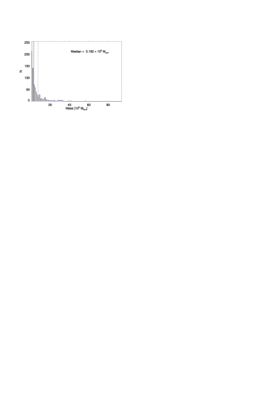
Figure 5: Predicted masses for the flare published by Mossoux et al. (2015), detected with XMM/Newton/Epic instrument.

Figure 6: Best fit for the flare published in Mossoux et al. (2015)

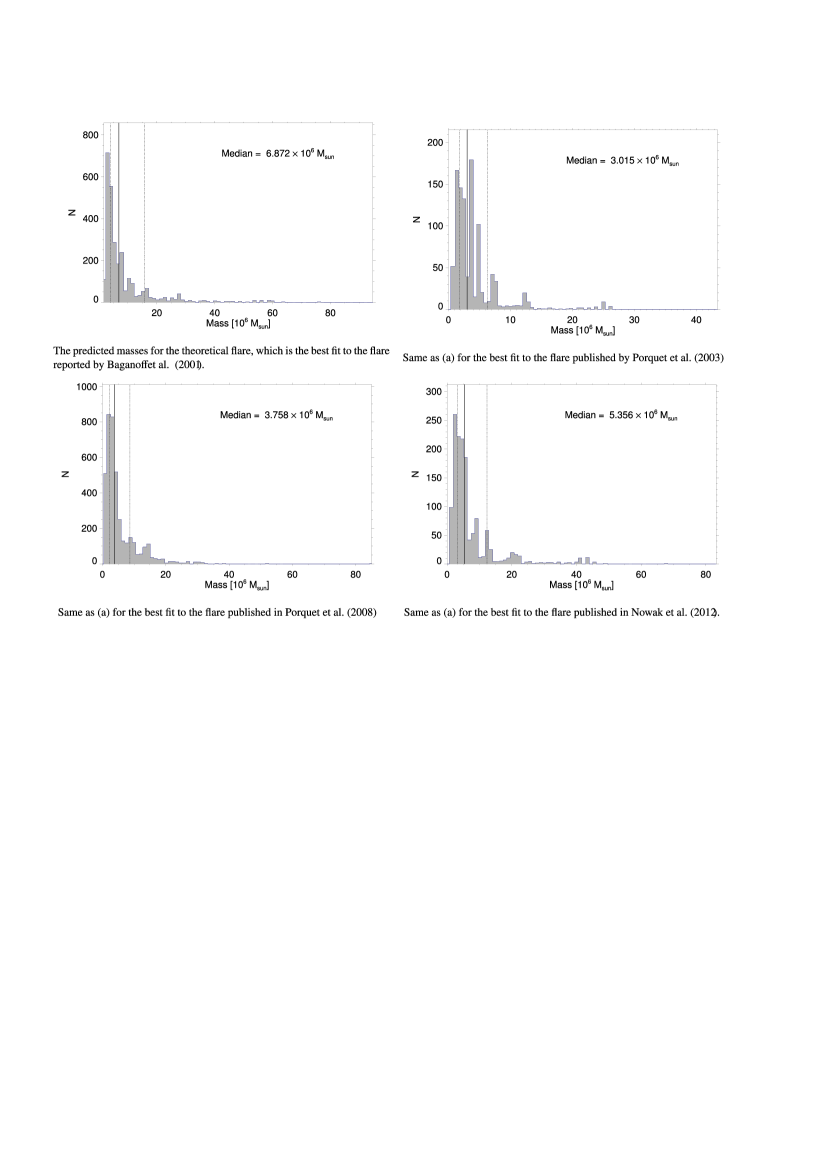
Figure 7:

5.3 Robustness of the method

The question remains, whether the median of the distribution of obtained is actually a good measure for the mass of the black hole or not. Therefore, we tested the method against artificial light curves and applied it to data of a different, extragalactic supermassive black hole.

5.3.1 Artificial flares

To investigate how accurate the proposed method of constraining the black hole mass is, we test the method against light curves that are produced by a black hole with a known mass. As we are probing models with the same routine we generate the test models with - this can only be a test of whether the median of the mass distribution is appropriated to derive the model input mass again. In this sense the test is only a consistency test of the input versus the output of the model. We used the best fits to the four flares, set the associated mass to a known value of $4\times 10^{6}M_{\odot}$. Here, it is only important is that a value was set. The results will scale with any mass value set differently. This leaves us with four theoretical light curves corresponding to a black hole of a known mass. Furthermore, each one of these light curves are the best fit of one of the observed flares. From these theoretical flares we extracted data on the same time support as the observed flares and applied our method to these artificial flares. The resulting mass diagrams are shown in Fig. 7. As a median mass value of the medians of the 4 artificial flares we obtain $M_{artif.,median}=(4.56\pm 0.80)\times 10^{6}M_{\odot}$. This agrees to within the uncertainties with the preset value of $4\times 10^{6}M_{\odot}$. Within 2 times the uncertainties it agrees with the $M_{SgrA*,median}=(3.49\pm 0.20)\times 10^{6}M_{\odot}$ result obtained for SgrA* with a measured mass of $(4.02\pm 0.17)\times 10^{6}M_{\odot}$ by Boehle et al. (2016), i.e., a value close to the preset mass. We conclude that mass can be determined with our new method with an accuracy between 5% and 20% (with a median value around 12%), and that in addition to detector noise the step width of the basic simulation parameters listed in Tab. 1 as well as the limited time support of the light curves is a main source of the uncertainties.

5.3.2 Applying the method to a different source

We also test the method on another X-ray source which displays a periodicity, RE J1034+396, a Seyfert I galaxy. Gierliński et al. (2008) and Middleton et al. (2009) have published observations of this source, that show a QPO with a duration of about 1 hour at X-ray frequencies. This QPO has further been confirmed by Vaughan (2010), who states that the detection was not as significant. Middleton et al. (2011) however, found no evidence of a periodic feature in the power spectral density, but cannot exclude a QPO in two low-flux observations. This prompts the conclusion, that the QPO might be a temporary feature. Alston et al. (2014) analyzed several observations of this source and found that this quasi period oscillation can be observed in five XMM-Newton observations. The authors further state, that the QPO can only be found when the source is in a low-flux state. Several authors have given estimates for the mass of this source (Gierliński et al., 2008; Bian & Huang, 2010; Jin et al., 2012), which are listed in Table 3. The fact that this source appears to exhibit QPOs particularly during low-flux phases, while it does not necessarily appear in all observations, suggests that this feature might arise from a similar mechanism as the flares of Sgr A*.

Czerny et al. (2010) find that the period of the QPO of this source appears to increase with increasing flux. Following their timing analysis, the authors exclude a hotspot model on the basis, that only a face on hotspot could explain the observations, which the authors do not find very probable.

We apply our hotspot model the same way as outlined for the X-ray flares of Sgr A*. The histogram of all resulting mass estimates is shown in Fig. 8 and the median mass is around $M_{RE~{}J1034+396}=1.421\times 10^{6}M_{\odot}$. The best fit to the light curve is shown in Fig. 9. This mass is consistent with the estimates of other authors, who have used different methods (cf. Table 3). The fact that only models with a very low inclination result in an acceptable fit, compares well with the observation that this particular source appears to only exhibit a QPO during low flux phases. As stated above, in our model the biggest magnification is achieved at high inclinations, because then the special as well as the general relativistic effects are most effective. The QPO of RE J1034+396 is actually only a modulation of $\sim 15\%$, whereas X-ray flares of Sgr A* can reach fluxes that are magnified by a factor of $>100$, when compared to the quiescent level. That is the reason why all flares of Sgr A* that were analyzed, compare better to models of high viewing angles, while the QPO of RE J1034+396 most likely results from a hotspot orbiting at a face on viewing angle with respect to the observer. Indeed, there are only three fits with a $\chi^{2}_{flare,red}<3$ in our analysis of this source, all of which are at a viewing angle of $5^{\circ}$. This is consistent with the conclusions of Czerny et al. (2010), even though we have employed a completely different method.

We conclude that this new way of estimating the mass of black holes gives results that are in agreement with those of independent methods. Not only is the estimated mass of the SMBH located at Sgr A* which results from this method consistent with those of previous publications, but it also yields a good mass estimate for the extragalactic source RE J1034+396.

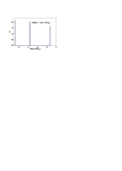
Figure 8: Weighted histogram for the QPO of J1034-396 as published by Gierliński et al. (2008)

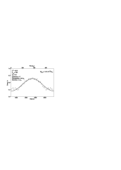
Figure 9: Best fit for the QPO of J1034-396 show for data of the folded light curve as published by Gierliński et al. (2008)

Table 3: Mass estimates of the Seyfert I galaxy RE J1034+396 with different methods in chronological order.

Publication	Mass	Method
Gierliński et al. (2008)	$6.3\times 10^{5}M_{\odot}$	$H\beta$
Gierliński et al. (2008)	$3.6\times 10^{7}M_{\odot}$	$[O{III}]$
Gierliński et al. (2008)	$(8\times 10^{6}-9\times 10^{7})M_{\odot}$	ISCO
Bian & Huang (2010)	$(1-4)\times 10^{6}M_{\odot}$	$M-\sigma_{*}$
Bian & Huang (2010)	$(1-4)\times 10^{6}M_{\odot}$	$H\beta$
Jin et al. (2012)	$1.7\times 10^{6}M_{\odot}$	$H\beta$
This paper	$1.421\times 10^{6}M_{\odot}$	hotspot

6 Summary

We have argued, that the double-peak structure of the X-ray flares observed from Sgr A* could arise from a simple orbiting hotspot model. In fact, only a fraction of a full orbit is needed to result in a light curve with double-peak profile. It is thus very probable that a hotspot can be stable long enough to create a flare.

We have outlined a method which makes use of a comparison of the simulations with the four brightest X-ray flares and gives an estimate on the mass of the black hole. The mass estimate is independent of the uncertainties about the object distance. The resulting masses are in close proximity to the other estimates of the supermassive black hole mass which must be located at the position of the radio source Sgr A*, which make use of stellar orbits. Clearly the method should be tested by applying it to other bright X-ray flares, observed in the future. By applying this model to more and more flares, the estimate for the mass should improve. A future X-ray polarimeter mission would make this method even more reliable, because the polarization parameters can be simulated with this model as well.

The method described here works only is the light curves of the flare events are dominated by the effects of relativistic motion of the luminous matter orbiting the black hole. Hence, this method also has possible applications to other sources which exhibit flares with a double-peak structure and could be used to get an estimate on the mass of the black holes of sources, when stellar orbits cannot be resolved. We also expect that the method works best on bright flares as these are statistically less frequent. For more frequent, faint flares an overlap between flare events is more likely and will therefore lead to less meaningful results.

7 Acknowledgements

We thank the referee for constructive comments and suggestions. We received funding from the European Union Seventh Framework Program (FP7/2007-2013) under grant agreement No. 312789 - Strong gravity: Probing Strong Gravity by Black Holes Across the Range of Masses. This work was supported in part by the Deutsche Forschungsgemeinschaft (DFG) via the Cologne Bonn Graduate School (BCGS), the Max Planck Society through the International Max Planck Research School (IMPRS) for Astronomy and Astrophysics, as well as special funds through the University of Cologne and SFB 956 - Conditions and Impact of Star Formation. M. Zajacek and B. Shahzamanian are members of the IMPRS. Part of this work was supported by fruitful discussions with members of the European Union funded COST Action MP0905: Black Holes in a Violent Universe and the Czech Science Foundation - DFG collaboration (No. 13-00070J). We thank the German Ministry of Education and Research (BMBF) for support under COPRAG2015 (No.57147386).

References

- Abramowicz et al. (1991) Abramowicz M. A., Bao G., Lanza A., Zhang X.-H., 1991, A&A, 245, 454
- Abramowicz et al. (1992) Abramowicz M. A., Lanza A., Spiegel E. A., Szuszkiewicz E., 1992, Nature, 356, 41
- Adams & Watkins (1995) Adams F. C., Watkins R., 1995, ApJ, 451, 314
- Alston et al. (2014) Alston W. N., Markevičiūtė J., Kara E., Fabian A. C., Middleton M., 2014, MNRAS, 445, L16
- Armitage & Reynolds (2003) Armitage P. J., Reynolds C. S., 2003, MNRAS, 341, 1041
- Baganoff et al. (2001) Baganoff F. K., et al., 2001, Nature, 413, 45
- Baganoff et al. (2003) Baganoff F. K., et al., 2003, ApJ, 591, 891
- Bahcall & Tremaine (1981) Bahcall J. N., Tremaine S., 1981, ApJ, 244, 805
- Balbus & Hawley (1991) Balbus S. A., Hawley J. F., 1991, ApJ, 376, 214
- Balick & Brown (1974) Balick B., Brown R. L., 1974, ApJ, 194, 265
- Bian & Huang (2010) Bian W.-H., Huang K., 2010, MNRAS, 401, 507
- Boehle et al. (2016) Boehle A., et al., 2016, ApJ, 830, 17
- Broderick & Loeb (2005) Broderick A. E., Loeb A., 2005, MNRAS, 363, 353
- Broderick & Loeb (2006) Broderick A. E., Loeb A., 2006, MNRAS, 367, 905
- Brown & Lo (1982) Brown R. L., Lo K. Y., 1982, ApJ, 253, 108
- Czerny et al. (2010) Czerny B., Lachowicz P., Dovčiak M., Karas V., Pecháček T., Das T. K., 2010, A&A, 524, A26
- Dai et al. (2010) Dai L. J., Fuerst S. V., Blandford R., 2010, MNRAS, 402, 1614
- Dexter & Agol (2009) Dexter J., Agol E., 2009, ApJ, 696, 1616
- Dodds-Eden et al. (2009) Dodds-Eden K., et al., 2009, ApJ, 698, 676
- Dovc̆iak (2004) Dovc̆iak M., 2004, PhD thesis, 2004, PhD Thesis, Charles University, Prague
- Eckart et al. (2002) Eckart A., Genzel R., Ott T., Schödel R., 2002, MNRAS, 331, 917
- Eckart et al. (2004) Eckart A., et al., 2004, A&A, 427, 1
- Eckart et al. (2006) Eckart A., Schödel R., Meyer L., Trippe S., Ott T., Genzel R., 2006, A&A, 455, 1
- Eckart et al. (2008) Eckart A., et al., 2008, A&A, 479, 625
- Eckart et al. (2012) Eckart A., et al., 2012, A&A, 537, A52
- Eckart et al. (2017) Eckart A., et al., 2017, Foundations of Physics, 47, 553
- Einstein (1905) Einstein A., 1905, Annalen der Physik, 322, 891
- Genzel et al. (1996) Genzel R., Thatte N., Krabbe A., Kroker H., Tacconi-Garman L. E., 1996, ApJ, 472, 153
- Genzel et al. (2003) Genzel R., Schödel R., Ott T., Eckart A., Alexander T., Lacombe F., Rouan D., Aschenbach B., 2003, Nature, 425, 934
- Ghez et al. (2003) Ghez A. M., et al., 2003, ApJ, 586, L127
- Ghez et al. (2004) Ghez A. M., et al., 2004, ApJ, 601, L159
- Gierliński et al. (2008) Gierliński M., Middleton M., Ward M., Done C., 2008, Nature, 455, 369
- Gillessen et al. (2009) Gillessen S., Eisenhauer F., Trippe S., Alexander T., Genzel R., Martins F., Ott T., 2009, ApJ, 692, 1075
- Haller et al. (1996) Haller J. W., Rieke M. J., Rieke G. H., Tamblyn P., Close L., Melia F., 1996, ApJ, 456, 194
- Hornstein et al. (2007) Hornstein S. D., Matthews K., Ghez A. M., Lu J. R., Morris M., Becklin E. E., Rafelski M., Baganoff F. K., 2007, ApJ, 667, 900
- Jalali et al. (2014) Jalali B., et al., 2014, MNRAS, 444, 1205
- Jin et al. (2012) Jin C., Ward M., Done C., Gelbord J., 2012, MNRAS, 420, 1825
- Lense & Thirring (1918) Lense J., Thirring H., 1918, Physikalische Zeitschrift, 19, 156
- Macquart et al. (2006) Macquart J.-P., Bower G. C., Wright M. C. H., Backer D. C., Falcke H., 2006, ApJ, 646, L111
- Markoff et al. (2001) Markoff S., Falcke H., Yuan F., Biermann P. L., 2001, A&A, 379, L13
- McGinn et al. (1989) McGinn M. T., Sellgren K., Becklin E. E., Hall D. N. B., 1989, ApJ, 338, 824
- Merritt et al. (2010) Merritt D., Alexander T., Mikkola S., Will C. M., 2010, Phys. Rev. D, 81, 062002
- Meyer et al. (2006a) Meyer L., Schödel R., Eckart A., Karas V., Dovčiak M., Duschl W. J., 2006a, A&A, 458, L25
- Meyer et al. (2006b) Meyer L., Eckart A., Schödel R., Duschl W. J., Mužić K., Dovčiak M., Karas V., 2006b, A&A, 460, 15
- Meyer et al. (2007) Meyer L., Schödel R., Eckart A., Duschl W. J., Karas V., Dovčiak M., 2007, A&A, 473, 707
- Middleton et al. (2009) Middleton M., Done C., Ward M., Gierliński M., Schurch N., 2009, MNRAS, 394, 250
- Middleton et al. (2011) Middleton M., Uttley P., Done C., 2011, MNRAS, 417, 250
- Mościbrodzka & Falcke (2013) Mościbrodzka M., Falcke H., 2013, A&A, 559, L3
- Mościbrodzka et al. (2009) Mościbrodzka M., Gammie C. F., Dolence J. C., Shiokawa H., Leung P. K., 2009, ApJ, 706, 497
- Mościbrodzka et al. (2014) Mościbrodzka M., Falcke H., Shiokawa H., Gammie C. F., 2014, A&A, 570, A7
- Mossoux et al. (2015) Mossoux E., Grosso N., Vincent F. H., Porquet D., 2015, A&A, 573, A46
- Mouawad et al. (2005) Mouawad N., Eckart A., Pfalzner S., Schödel R., Moultaka J., Spurzem R., 2005, Astronomische Nachrichten, 326, 83
- Neilsen et al. (2015) Neilsen J., et al., 2015, ApJ, 799, 199
- Nishiyama et al. (2009) Nishiyama S., Tamura M., Hatano H., Nagata T., Kudo T., Ishii M., Schödel R., Eckart A., 2009, ApJ, 702, L56
- Nowak et al. (2012) Nowak M. A., et al., 2012, ApJ, 759, 95
- Porquet et al. (2003) Porquet D., Predehl P., Aschenbach B., Grosso N., Goldwurm A., Goldoni P., Warwick R. S., Decourchelle A., 2003, A&A, 407, L17
- Porquet et al. (2008) Porquet D., et al., 2008, A&A, 488, 549
- Poutanen & Fabian (1999) Poutanen J., Fabian A. C., 1999, MNRAS, 306, L31
- Reid & Brunthaler (2004) Reid M. J., Brunthaler A., 2004, ApJ, 616, 872
- Rieke & Rieke (1988) Rieke G. H., Rieke M. J., 1988, ApJ, 330, L33
- Schnittman (2005) Schnittman J. D., 2005, ApJ, 621, 940
- Schnittman et al. (2006) Schnittman J. D., Krolik J. H., Hawley J. F., 2006, ApJ, 651, 1031
- Schödel et al. (2002) Schödel R., et al., 2002, Nature, 419, 694
- Sellgren et al. (1990) Sellgren K., McGinn M. T., Becklin E. E., Hall D. N., 1990, ApJ, 359, 112
- Stella & Vietri (1998) Stella L., Vietri M., 1998, ApJ, 492, L59
- Stella & Vietri (1999) Stella L., Vietri M., 1999, Physical Review Letters, 82, 17
- Trippe et al. (2007) Trippe S., Paumard T., Ott T., Gillessen S., Eisenhauer F., Martins F., Genzel R., 2007, MNRAS, 375, 764
- Vaughan (2010) Vaughan S., 2010, MNRAS, 402, 307
- Witzel et al. (2014) Witzel G., et al., 2014, in Sjouwerman L. O., Lang C. C., Ott J., eds, IAU Symposium Vol. 303, IAU Symposium. pp 274–282, doi:10.1017/S1743921314000738
- Wollman et al. (1977) Wollman E. R., Geballe T. R., Lacy J. H., Townes C. H., Rank D. M., 1977, ApJ, 218, L103
- Yuan et al. (2004) Yuan F., Quataert E., Narayan R., 2004, ApJ, 606, 894
- Yuan et al. (2009) Yuan F., Lin J., Wu K., Ho L. C., 2009, MNRAS, 395, 2183
- Yusef-Zadeh et al. (2006) Yusef-Zadeh F., et al., 2006, ApJ, 644, 198
- Yusef-Zadeh et al. (2009) Yusef-Zadeh F., et al., 2009, ApJ, 706, 348
- Zamaninasab et al. (2010) Zamaninasab M., et al., 2010, A&A, 510, A3
- Zamaninasab et al. (2011) Zamaninasab M., et al., 2011, MNRAS, 413, 322
- Życki (2002) Życki P. T., 2002, MNRAS, 333, 800