Solar Radiation Pressure Resonances in Low Earth Orbits

Abstract

The aim of this work is to highlight the crucial role that orbital resonances associated with solar radiation pressure can have in Low Earth Orbit. We review the corresponding literature, and provide an analytical tool to estimate the maximum eccentricity which can be achieved for well-defined initial conditions. We then compare the results obtained with the simplified model with the results obtained with a more comprehensive dynamical model. The analysis has important implications both from a theoretical point of view, because it shows that the role of some resonances was underestimated in the past, but also from a practical point of view in the perspective of passive deorbiting solutions for satellites at the end-of-life.

1 Introduction

It is known that the effect of the solar radiation pressure (SRP) on the orbital motion is a long-period variation in eccentricity $e$ and inclination $i$, along with one in longitude of ascending node $\Omega$ and argument of pericenter $\omega$, and that the magnitude of this variation depends on the area-to-mass ratio of the body (e.g., Beutler, 2005). If we assume a perturbing potential which is averaged over the orbital period of the body, the SRP effect can be subject to resonances, associated with a commensurability among the rate of precession of the ascending node, the one of the argument of pericenter and the mean apparent motion of the Sun, say $n_{S}$. As well-known, when a resonance occurs, the period of the variation can become so large to give rise to quasi-secular effects in the corresponding orbital element.

Motivated by the numerical results (Alessi et al., 2017a, b) obtained recently within the ReDSHIFT H2020 project (Rossi et al., 2017), the aim of this work is to describe the role of SRP resonances in the Low Earth Orbit (LEO) region, showing that their contribution can provide relatively significant eccentricity variations.

In the past, the effect of the solar radiation pressure for orbits around the Earth was considered mainly in the perspective of bodies characterised by a very high area-to-mass ratio. We can mention works focused on the behaviour of Geostationary Earth Orbits (GEO) (e.g., Valk et al., 2007; Rosengren & Scheeres, 2013; Casanova et al., 2015), or on mission concepts aiming to exploit a solar sail to deorbiting non-operational objects from Medium Earth Orbits (MEO) (e.g., Lücking et al., 2012), or on the design of frozen orbits for small-size objects (e.g., Colombo et al., 2012; Lantukh et al., 2015). Colombo et al. (2012), in particular, analysed SRP effects on high area-to-mass objects in order to design frozen orbits for a swarm of small spacecraft dedicated to Earth observation and telecommunication purposes. Starting from the work by Krivov et al. (1996), they studied the behaviour in eccentricity corresponding to $\dot{\Omega}+\dot{\omega}-n_{S}=0$, by computing the equilibrium points, and their stability, in a dynamical system including the oblateness of the Earth and SRP.

From a theoretical point of view, the first works on the resonances induced by SRP started from the analysis of the resonances induced by the solar gravitational attraction. As a matter of fact, the two disturbing potentials differ in the first order of the expansion and in the amplitude of the perturbation (Hughes, 1977). If we focus on the resonances affecting the eccentricity evolution, Musen (1960) and Cook (1962) were the first to highlight the existence of six SRP resonances, and to show their location in the $(i,a)$ plane. Cook (1962), in particular, noted that, contrary to lunisolar gravitational resonances, the SRP resonances are able to give a variation in eccentricity also in the case of circular orbits. Musen (1960) labelled $\dot{\Omega}+\dot{\omega}-n_{S}$ as the ‘most interesting resonance’, as done by all the following authors. In the case of the gravitational perturbation, this resonance is also known as evection resonance (e.g., Brouwer & Clemence, 1961; Touma & Widsom, 1998; Frouard et al., 2010). Breiter (1999), basing his analysis on the work done by Cook (1962), noted that ‘resonant solar perturbations can be much stronger than the lunar ones’. He also considered $\dot{\Omega}+\dot{\omega}-n_{S}$ as the dominant resonance for prograde orbits and $\dot{\Omega}-\dot{\omega}+n_{S}$ for retrograde orbits. In his work, the strength of a given resonance is determined by the magnitude of the libration region. As already mentioned, a fundamental contribution to the topic was given by Hughes (Hughes, 1977, 1980, 1981), who tried to provide a more general treatment to the problem, by analysing also the effect due to high-order terms. He stressed that SRP resonances give rise to variations not only in eccentricity, but also in inclination, longitude of the ascending node and argument of pericenter. He considered a resonance as dominant according to the magnitude of the corresponding amplitude, function of semi-major axis $a$ and eccentricity. More recently, Celletti et al. (2017) recognised the occurrence of semi-secular resonances, as the SRP ones, in the LEO region, but they stated that ‘Since the semi-secular resonances occur at specific altitudes, the width of such resonances is small, and since the air drag provokes a decay of the orbits on relatively short time scales, one expects that these resonances play a minor role in the long-term evolution of space debris’. We will show that this is partially true. Though the regions where SRP resonances are effective are indeed narrow, for high values of area-to-mass ratio, they represent the main mechanism to drive a satellite back to the Earth also when the LEO is sufficiently high to have a negligible interaction with the residual atmosphere, e.g., above an altitude $h\simeq 1000$ km. On the other hand, if we consider low values of area-to-mass ratio, the combined effect of the atmospheric drag and the SRP resonances can reduce significantly the lifetime of the object.

One of the fundamental issue to mitigate the space debris problem and control the growth of the debris population is to see if there exist natural perturbations which facilitate the reentry to the Earth or, when this is not possible, ensure a stable graveyard orbit in the long-term. At altitudes when the atmospheric drag is not effective, the only way to lower the pericenter altitude is to obtain an eccentricity increase. For MEO, like those of the GNSS constellations, the gravitational lunisolar perturbations can help to this end too (Rosengren et al., 2015; Alessi et al., 2016). In LEO, apart from the atmospheric drag, the main natural effects that can be exploited are the lunisolar gravitational resonance, in particular the one corresponding to $\dot{\Omega}+2\dot{\omega}$ (Alessi et al., 2017a, b) and the SRP. In particular, as just mentioned, area-to-mass values representing small spacecraft equipped with a solar sail can experience a change as dramatic as to reenter to the Earth, even without the support of the atmospheric drag. These situations occur in correspondence of the $\dot{\Omega}+\dot{\omega}-n_{S}$ resonance, considered as dominant in the past, but not only. On the other hand, understanding how the eccentricity might change due to the SRP is crucial also to control the stability of a graveyard orbit.

As a final note, we acknowledge that looking for the values of area-to-mass ratio ensuring a reentry, given initial semi-major axis and inclination, Colombo & de Bras de Fer (2016) found numerically the same reentry corridors represented by at least two of the six SRP resonances, that will be described here.

2 The Model

Let us assume that the radiation coming from the Sun is directed normally to the surface of the spacecraft, that is, the so-called cannonball model. Moreover, let us assume the orbit of the spacecraft entirely in the sunlight, and the effect of Earth’s albedo as negligible.

Neglecting the light aberration, the solar radiation pressure is a conservative force. The corresponding disturbing potential, averaged over the orbital motion of the spacecraft, can be written as (e.g., Krivov et al., 1996)

$${\mathcal{R}}_{SRP} = \frac{3}{2}PC_{R}\frac{A}{m}ae[\cos\omega\left(\cos\Omega\cos\lambda_{S}+\sin\Omega\sin\lambda_{S}\cos\epsilon\right)$$

$$+\sin\omega\left(\cos\Omega\cos i\sin\lambda_{S}\cos\epsilon-\sin\Omega\cos i\cos\lambda_{S}\right)$$

$$+\sin i\sin\omega\sin\lambda_{S}\sin\epsilon],$$

$$= \frac{3}{2}PC_{R}\frac{A}{m}ae[\mathcal{T}_{1}\cos\psi_{1}+\mathcal{T}_{2}\cos\psi_{2}+\mathcal{T}_{3}\cos\psi_{3}+$$

$$\mathcal{T}_{4}\cos\psi_{4}+\mathcal{T}_{5}\cos\psi_{5}+\mathcal{T}_{6}\cos\psi_{6}],$$

where $\lambda_{S}$ is the longitude of the Sun measured on the ecliptic plane, $\epsilon=23.439^{\circ}$ is the obliquity of the ecliptic, $P$ the solar radiation pressure , $C_{R}$ the reflectivity coefficient, $A/m$ the area-to-mass ratio,

$$\psi_{j}=n_{1}\Omega+n_{2}\omega+n_{3}\lambda_{S},$$ (2)

with $n_{1}=\{0,1\}$, $n_{2}=\pm 1$, $n_{3}=\pm 1$, according to $j$, following Table 1, and

$$\mathcal{T}_{1} = \cos^{2}\left(\frac{\epsilon}{2}\right)\cos^{2}\left(\frac{i}{2}\right)$$

$$\mathcal{T}_{2} = \cos^{2}\left(\frac{\epsilon}{2}\right)\sin^{2}\left(\frac{i}{2}\right)$$

$$\mathcal{T}_{3} = \frac{1}{2}\sin(\epsilon)\sin(i)$$ (3)

$$\mathcal{T}_{4} = -\frac{1}{2}\sin(\epsilon)\sin(i)$$

$$\mathcal{T}_{5} = \sin^{2}\left(\frac{\epsilon}{2}\right)\cos^{2}\left(\frac{i}{2}\right)$$

$$\mathcal{T}_{6} = \sin^{2}\left(\frac{\epsilon}{2}\right)\sin^{2}\left(\frac{i}{2}\right).$$

Table 1: Resonance $\psi_{j}=n_{1}\Omega+n_{2}\omega+n_{3}\lambda_{S}$ in terms of $n_{1},n_{2},n_{3}$.

$j$	$n_{1}$	$n_{2}$	$n_{3}$
1	1	1	-1
2	1	-1	-1
3	0	1	-1
4	0	1	1
5	1	1	1
6	1	-1	1

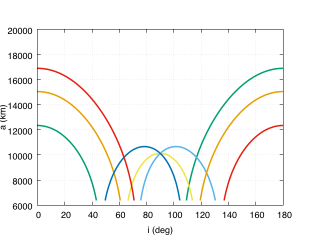
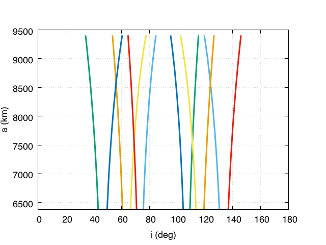
Figure 1: On the top, we show the location of the six main SRP resonances as a function of $i,a$ for $e=0.01$. On the bottom, a close-up in the LEO region, defined here up to $h=3000$ km, in order to account also for possible graveyard orbits. The curves were computed assuming $\dot{\Omega}=\dot{\Omega}_{J_{2}}$ and $\dot{\omega}=\dot{\omega}_{J_{2}}$. Green: $\dot{\Omega}+\dot{\omega}-n_{S}=0$. Cyan: $\dot{\Omega}-\dot{\omega}-n_{S}=0$. Orange: $\dot{\omega}-n_{S}=0$. Yellow: $\dot{\omega}+n_{S}=0$. Blue: $\dot{\Omega}+\dot{\omega}+n_{S}=0$. Red: $\dot{\Omega}-\dot{\omega}+n_{S}=0$.

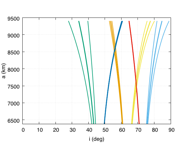
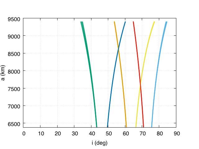
Figure 2: Location of the six main SRP resonances as a function of $i,a$ for $e=0.01$ (top) and $e=0.1$ (bottom) in the LEO region for prograde orbits for $A/m=1$ m${}^{2}/$kg. The curves were computed assuming $\dot{\Omega}=\dot{\Omega}_{J_{2}}+\dot{\Omega}_{SRP}$ and $\dot{\omega}=\dot{\omega}_{J_{2}}+\dot{\omega}_{SRP}$. Green: $\dot{\Omega}+\dot{\omega}-n_{S}=0$. Cyan: $\dot{\Omega}-\dot{\omega}-n_{S}=0$. Orange: $\dot{\omega}-n_{S}=0$. Yellow: $\dot{\omega}+n_{S}=0$. Blue: $\dot{\Omega}+\dot{\omega}+n_{S}=0$. Red: $\dot{\Omega}-\dot{\omega}+n_{S}=0$. For a given resonance, the middle curve corresponds to $\psi=90^{\circ}$. If $n_{3}=1$ the right curve corresponds to $\psi=0^{\circ}$, the left one to $\psi=180^{\circ}$; if $n_{3}=-1$ viceversa.

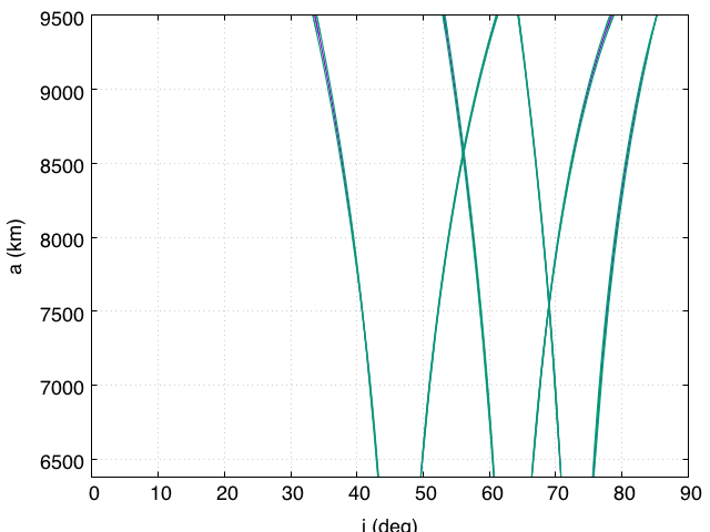
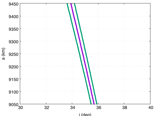
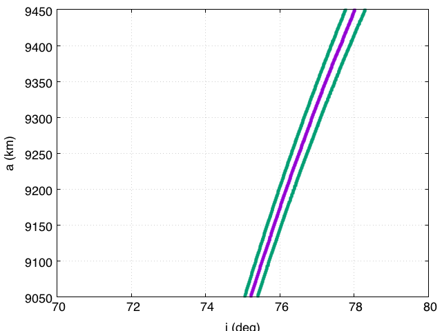
Figure 3: Resonance width, computed for $e=0.01$ and $A/m=1$ m${}^{2}/$kg. The middle and right panels show the regions where the width computed is the largest: they correspond to resonance #1 and resonance #3, respectively.

If we assume that the dynamics is driven by a single resonance, then we can write the variation in the orbital elements as due to only one, say $j$, of the terms in (2) at a time. By applying the Lagrange planetary equations, we get

$$\frac{de}{dt} = -\frac{3}{2}PC_{R}\frac{A}{m}\frac{\sqrt{1-e^{2}}}{na}\mathcal{T}_{j}{\partial{\cos{\psi}_{j}}\over\partial\omega}$$ (4)

$$\frac{di}{dt} = -\frac{3}{2}PC_{R}\frac{A}{m}\frac{e}{na\sqrt{1-e^{2}}\sin i}\mathcal{T}_{j}\left({\partial{\cos{\psi}_{j}}\over\partial\Omega}-\cos i{\partial{\cos{\psi}_{j}}\over\partial\omega}\right)$$

$$\frac{d\Omega}{dt} = \dot{\Omega}_{J_{2}}+\dot{\Omega}_{SRP}$$

$$\frac{d\omega}{dt} = \dot{\omega}_{J_{2}}+\dot{\omega}_{SRP},$$

where $n$ is the mean motion of the satellite and we have assumed that the only other effect exerting a perturbation on the spacecraft is the oblateness of the Earth. We have

$$\dot{\Omega}_{J_{2}} = -\frac{3}{2}\frac{J_{2}r^{2}_{\bigoplus}n}{a^{2}(1-e^{2})^{2}}\cos i$$ (5)

$$\dot{\Omega}_{SRP} = \frac{3}{2}PC_{R}\frac{A}{m}\frac{e}{na\sqrt{1-e^{2}}\sin i}{\partial{\mathcal{T}}_{j}\over\partial i}\cos{\psi}_{j}$$

$$\dot{\omega}_{J_{2}} = \frac{3}{4}\frac{J_{2}r^{2}_{\bigoplus}n}{a^{2}(1-e^{2})^{2}}\left(5\cos^{2}i-1\right)$$

$$\dot{\omega}_{SRP} = \frac{3}{2}PC_{R}\frac{A}{m}\left(\frac{\sqrt{1-e^{2}}}{nae}\mathcal{T}_{j}\cos{\psi}_{j}-\frac{e\cos i}{na\sqrt{1-e^{2}}\sin i}{\partial{\mathcal{T}}_{j}\over\partial i}\cos{\psi}_{j}\right),$$

where $J_{2}$ is the second zonal term of the geopotential and $r_{\bigoplus}$ the equatorial radius of the Earth. The effect of lunisolar perturbations on $\dot{\Omega},\dot{\omega}$ can be neglected, following, e.g., Milani et al. (1987).

Notice that long-period and secular effects associated with the oblateness of the Earth affect only the behaviour of the longitude of the ascending node, of the argument of pericenter and of the mean anomaly. That is, the eccentricity does not change in the long-term due to $J_{2}$ (see, e.g., Roy (1982)).

3 The Eccentricity Resonances

From Eq. (4), we can recognise the following 6 resonances affecting the behaviour in eccentricity

$$\dot{\psi}_{j}=n_{1}\dot{\Omega}+n_{2}\dot{\omega}+n_{3}n_{S}=0.$$ (6)

In Fig. 1 we show their location as a function of the inclination and semi-major axis, for given values of $e$ and $A/m$, assuming that only the oblateness of the Earth is responsible of a variation in $\Omega$ and $\omega$. This approximation can be considered valid for $A/m=0.012$ m${}^{2}/$kg, which represents the average value of the intact objects orbiting in LEO. On the bottom panel, we show a close-up in the LEO region, defined here up to $h=3000$ km, in order to account also for possible graveyard orbits. Note that we prefer to represent the resonances as a function of $i,a$ instead of $a,e$, as done, e.g., in Colombo & McInnes (2012), because we focus on values of eccentricity which represent orbits of operational spacecraft in LEO. Realistic values cannot exceed the value $e=0.15$, the majority of the population in LEO having actually $e<0.02$. In general, except in the cases where the spacecraft is orbiting in a region where the atmospheric drag is dominant, or at a given resonance affecting the eccentricity evolution, the eccentricity can be assumed to vary in a negligible way with respect to the initial value. Also, in case of resonance, the timescale variation of the eccentricity is much slower than the typical period of the orbits considered.

In Fig.  2, we show the location of the same resonances for two different values of eccentricity, accounting also for the variation of $\Omega$ and $\omega$ due to SRP. In this case, the location of the resonances depends also on $\Omega,\omega,\lambda_{S}$. In the Figure we compute the curves corresponding to $\psi=0^{\circ},90^{\circ},180^{\circ}$ for $A/m=1$ m${}^{2}/$kg which represents a feasible value, given the current level of technology, for a small spacecraft equipped with a SRP enhancing device (see Colombo et al. (2017)). For a given resonance, the middle curve corresponds to the case $\psi=90^{\circ}$, which is equivalent to the case of Fig. 1. The displacement among the curves of a same resonance can be appreciated at higher LEO, for quasi-circular orbits for the first and the second resonance, following the convention in Table 1. Notice, however, that the first equation in (4) states that $\psi=0^{\circ}$ and $\psi=180^{\circ}$ are stationary points for the eccentricity, and thus we expect to have a quasi-secular behaviour in eccentricity only at approaching the condition $\psi=90^{\circ}$.

In the same Figures, we note that resonances of different nature can cross each other. Focusing on prograde LEO, there exist two main overlapping between SRP resonances. For quasi circular orbits, i.e., $e=0.01$, we have

• an overlapping between $\dot{\psi}=\dot{\omega}-n_{S}=0$ and $\dot{\psi}=\dot{\Omega}+\dot{\omega}+n_{S}=0$ at $a\approx r_{\bigoplus}+2193$ km and $i\approx 56.06^{\circ}$;

• an overlapping between $\dot{\psi}=\dot{\omega}+n_{S}=0$ and $\dot{\psi}=\dot{\Omega}-\dot{\omega}+n_{S}=0$ at $a\approx r_{\bigoplus}+1180$ km and $i\approx 69^{\circ}$.

Increasing the eccentricity, the value of the semi-major axis at which the crossing appears also increases, e.g., for $e=0.1$ the first crossing occurs at $a\approx r_{\bigoplus}+2245$ km, the second at $a\approx r_{\bigoplus}+1220$ km. From preliminary simulations, the dynamics at the overlapping does not manifest a chaotic behaviour, rather the two resonances concur to a possible increase in eccentricity. In general, we can observe isolated points where the Lyapunov time is significantly lower than that in the neighbourhood. They do not affect the overall dynamics, but they can be, however, object of further dedicated studies.

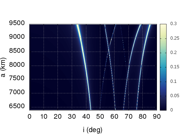
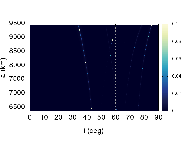
Figure 4: Maximum variation in eccentricity (color bar) that can be obtained along a given SRP resonance as a function of $i,a$ for $e=0.01$, $\Omega=0^{\circ}$, $\omega=0^{\circ}$, $\lambda_{S}=90.086^{\circ}$. Left: $A/m=1$ m${}^{2}/$kg. Right: $A/m=0.012$ m${}^{2}/$kg. See further details in the text.

To compute the width of the resonances considered, it can be applied the same argument developed by Daquin et al. (2016) for lunisolar doubly-averaged gravitational perturbations. Let us assume that the Hamiltonian function of the system is

$$\mathcal{H}=\mathcal{H}_{K}+\mathcal{H}_{J_{2}}+\mathcal{H}_{SRP},$$ (7)

where $\mathcal{H}_{K}$ is the Keplerian part, $\mathcal{H}_{J_{2}}$ the one associated with the oblateness of the Earth, and $\mathcal{H}_{SRP}=-{\mathcal{R}}_{SRP}$. The curves defining the boundaries of a given resonance $j$ at $X^{*}\equiv(e^{*},i^{*})$ are defined by the condition

$$n_{1}\dot{\Omega}+n_{2}\dot{\omega}+n_{3}n_{S}=\pm 2\sqrt{\nu}\left({\partial^{2}\mathcal{H}^{sec}\over\partial X^{2}}\right)_{|X=X^{*}},$$ (8)

where

$$\nu=\left|\frac{\frac{3}{2}PC_{R}\frac{A}{m}ae\mathcal{T}_{j}}{\left({\partial^{2}\mathcal{H}^{sec}\over\partial X^{2}}\right)_{|X=X^{*}}}\right|,$$ (9)

and ${\partial^{2}\mathcal{H}^{sec}\over\partial X^{2}}$ as in Daquin et al. (2016). For the sake of clarity,

$${\partial^{2}\mathcal{H}^{sec}\over\partial X^{2}}=\frac{3}{2}\frac{J_{2}r^{2}_{\bigoplus}}{a^{2}(1-e^{2})^{5/2}}\left[n_{2}^{2}\left(2-15\cos^{2}{i}\right)+10n_{1}n_{2}\cos i-n_{1}^{2}\right].$$

The width computed in this way turns out to be very narrow. In Figure 3, we provide an example for $A/m=1$ m${}^{2}/$kg, with a close-up in the regions where the width is the largest. Notice that they correspond to resonances #1 and #3.

With respect to a possible ranking of the six resonances in terms of the effect they might produce, the maximum eccentricity variation that can be achieved at a resonance $j$ can be estimated by integrating the first equation in (4). This is,

$$\Delta e=\left|\frac{3}{2}PC_{R}\frac{A}{m}\frac{\sqrt{1-e^{2}}}{na}\frac{\mathcal{T}_{j}}{\dot{\psi}_{j}}\right|.$$ (10)

In Fig. 4 we show the corresponding values as a function of $i,a$ for $e=0.01$, $\Omega=0^{\circ}$, $\omega=0^{\circ}$, $\lambda_{S}=90.086^{\circ}$ and $A/m=1$ m${}^{2}/$kg and $A/m=0.012$ m${}^{2}/$kg, sampling the $(i,a)$ plane at a step of $\Delta i=0.2^{\circ}$ and $\Delta a=20$ km. In the former case, the color bar representing the maximum eccentricity variation achievable is bounded to $0.3$, which is the value required to reenter from the highest LEO considered. In the latter case, the limit is set to $0.1$ just for the sake of clarity, that is, to be able to appreciate different behaviours, given the extreme narrowness of the resonances. For $A/m=0.012$ m${}^{2}/$kg, it should be noted that the variation that can be obtained is weak, and that, by definition of resonance, the time to get to the peak value is significantly long. Also, given that the range giving the required combination of inclination and semi-major axis is tapered, a possible exploitation of these corridors for an operational satellite would require an accurate manoeuvring capacity. A similar argument applies for resonance $\#6$ for $A/m=1$ m${}^{2}/$kg.

Note also that the same expression, Eq. (10), can be used to quantify the maximum possible change in eccentricity in the neighborhood of a given resonance, eventually avoiding an unrealistic operational time. This application is faced in detail in Schettino et al. (2017). We remark here that, for the strongest resonances (#1, #2 and #3), the range of initial inclinations that can be targeted to achieve a considerable change in eccentricity for the high area-to-mass case is generally at most $\pm 1^{\circ}$ with respect to the resonant value $i^{*}$, for given initial semi-major axis and eccentricity.

4 Numerical Evidence

The analysis described in the previous Section was compared to the results of the numerical simulations performed under the ReDSHIFT H2020 project (Rossi et al., 2017; Alessi et al., 2017a, b). The aim of the simulations was to map the whole LEO region in terms of initial orbital elements, considering two initial epochs and the same two values of area-to-mass ratio considered here, in order to look for natural deorbiting solutions that may facilitate the compliance with the international mitigation guidelines. A well-defined grid of initial conditions was propagated for 120 years by means of the semi-analytical orbital propagator FOP (Anselmo et al., 1996; Rossi et al., 2009), including in the dynamical model the geopotential up to degree and order 5, SRP, lunisolar perturbations and atmospheric drag below an altitude of 1500 km. The grid in initial inclination, in particular, was set at steps of $2^{\circ}$ in the range $[2^{\circ}:120^{\circ}]$.

In Fig. 5, we show the maximum eccentricity achieved in 120 years, as a function of initial inclination and eccentricity, starting from three different values of semi-major axis ($a=r_{\bigoplus}+1200$ km, $a=r_{\bigoplus}+1360$ km, $a=r_{\bigoplus}+1580$ km), for quasi-circular orbits, with a same initial configuration, and assuming $A/m=1$ m${}^{2}/$kg. It is possible to appreciate that the eccentricity can experience a non-negligible variation, only in correspondence of well-defined inclination bands (the brighter ones). These inclinations are located in the neighbourhood of the resonant values, described in the previous Section. In other words, within the limit of the grid adopted, only at resonant inclination values, the eccentricity can naturally increase.

It is also interesting to note that in the three examples the role of the dominant resonance, that is the one providing the greatest variation, changes. This is what we have called a resonance switching. In the top panel, this role is taken by resonance #2; in the middle by resonance #1; in the bottom by resonances #1 and #3.

In Fig. 6, we compare the maximum eccentricity computed with the numerical simulation with the maximum variation obtained using estimate (10), for the same three initial conditions as in Fig. 5, considering $e=0.01$ as initial eccentricity. The analytical value depicted is the sum of the six variations forecast by Eq. (10) for each resonance. This choice turned out to approximate better the actual behaviour of the maximum eccentricity, especially in the inclination regions between two resonant values. Given that in the simulations carried out with FOP other perturbations played a role and that the atmospheric drag was included, we consider that there exists a reasonable consistency between the numerical model and the simplified estimation. The resonance switching can also find an explanation, looking to the relative height corresponding to the cyan points, in particular for the first two examples.

In general, for all the cases explored, it turned out that also resonance #4 can yield a significant eccentricity variation, for the high area-to-mass value. See Fig. 7 for two examples.

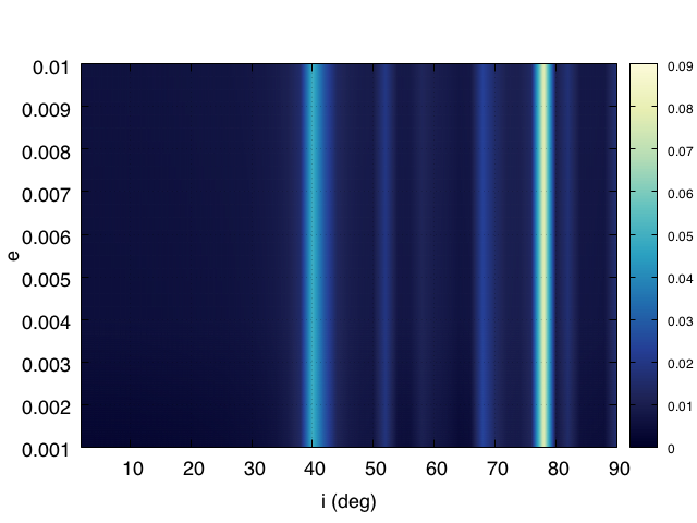
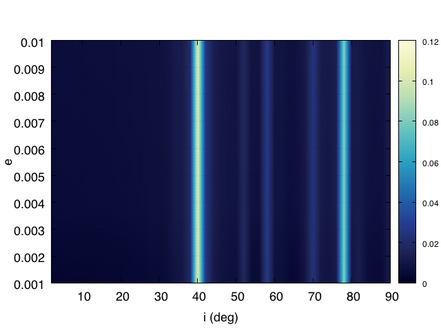
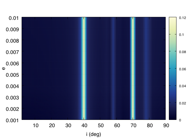
Figure 5: Maximum eccentricity (color bar) computed over 120 years with FOP, as a function of the initial inclination and eccentricity for $A/m=1$ m${}^{2}/$kg, starting from $\Omega=0^{\circ}$, $\omega=0^{\circ}$ on June 21, 2020 at 06:43:12 (i.e., $\lambda_{S}\approx 90.086^{\circ}$). Top: $a=r_{\bigoplus}+1200$ km; middle: $a=r_{\bigoplus}+1360$ km; bottom: $a=r_{\bigoplus}+1580$ km.

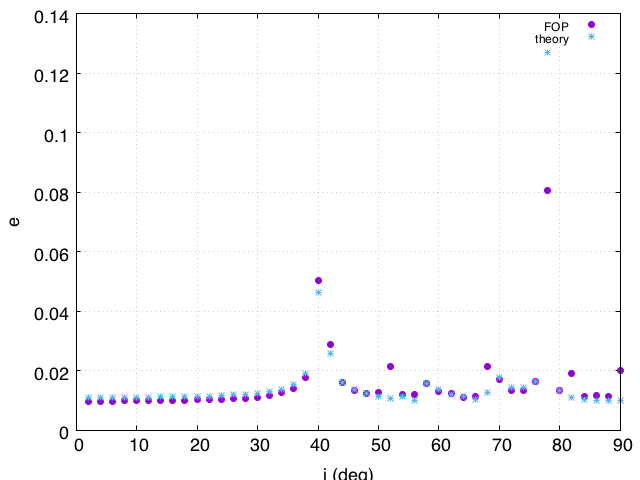
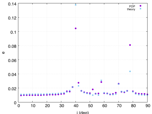
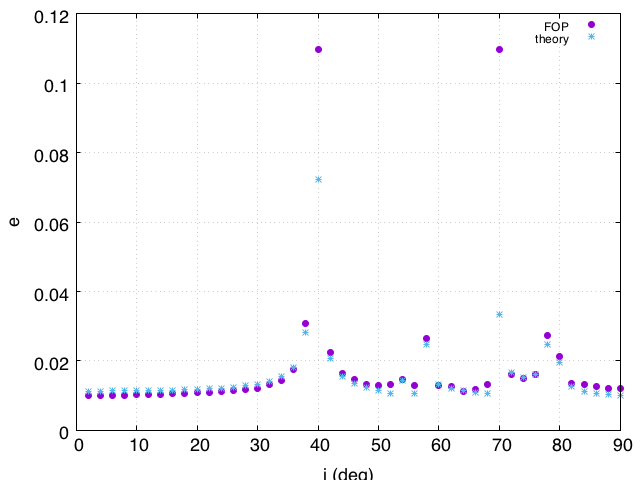
Figure 6: Maximum eccentricity computed over 120 years with FOP in purple, and following Eq. (10) in cyan, as a function of the initial inclination, for $A/m=1$ m${}^{2}/$kg, starting from $e=0.01$, $\Omega=0^{\circ}$, $\omega=0^{\circ}$ on June 21, 2020 at 06:43:12 (i.e., $\lambda_{S}\approx 90.086^{\circ}$). Top: $a=r_{\bigoplus}+1200$ km; middle: $a=r_{\bigoplus}+1360$ km; bottom: $a=r_{\bigoplus}+1580$ km.

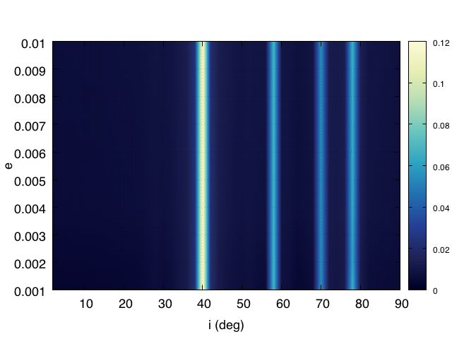
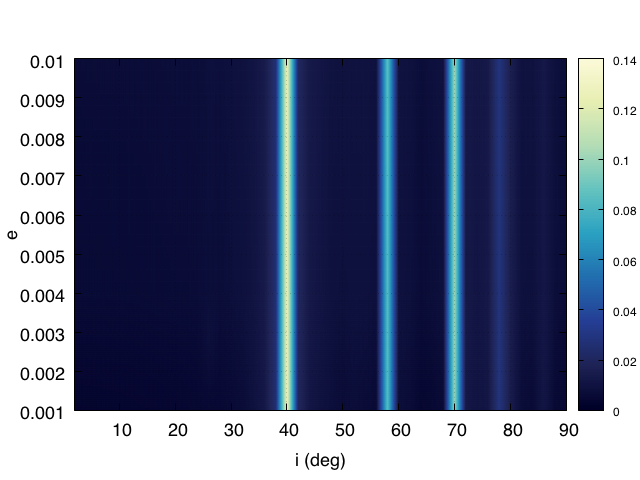
Figure 7: Maximum eccentricity (color bar) computed over 120 years with FOP, as a function of the initial inclination and eccentricity for $A/m=1$ m${}^{2}/$kg, starting from $a=r_{\bigoplus}+1460$ km (left) and $a=r_{\bigoplus}+1520$ km (right). In both cases, $\Omega=0^{\circ}$, $\omega=180^{\circ}$ on June 21, 2020 at 06:43:12 (i.e., $\lambda_{S}\approx 90.086^{\circ}$).

For $A/m=0.012$ m${}^{2}/$kg, in Figs. 8–9 we provide two examples of the eccentricity evolution and the consequent variation in the pericenter altitude by propagation with FOP, for altitudes where the atmospheric drag is not effective. They correspond to quasi-circular orbits, which are located at the resonance $\#2$ and $\#1$, respectively, at the initial epoch. We note the variation of hundreds of km obtained, but also the long time required. In Fig. 10, we show an example when the SRP resonance aids the action of the atmospheric drag. Starting from $i=41.95^{\circ}$, the reentry is achieved in about 55 years; starting from $i=42^{\circ}$, the lifetime is reduced by about 8 years. This shows that if the satellite is located in the neighbourhood of a SRP resonance, it could be worth to increase a little the eccentricity to clearing the region more rapidly. In this way, we can take advantage of both putting the spacecraft in a denser layer of the atmosphere and the push in eccentricity given by SRP, which can lower the pericenter altitude in the long-term. An accurate modelling of the interaction between SRP and atmospheric drag will be faced in the future.

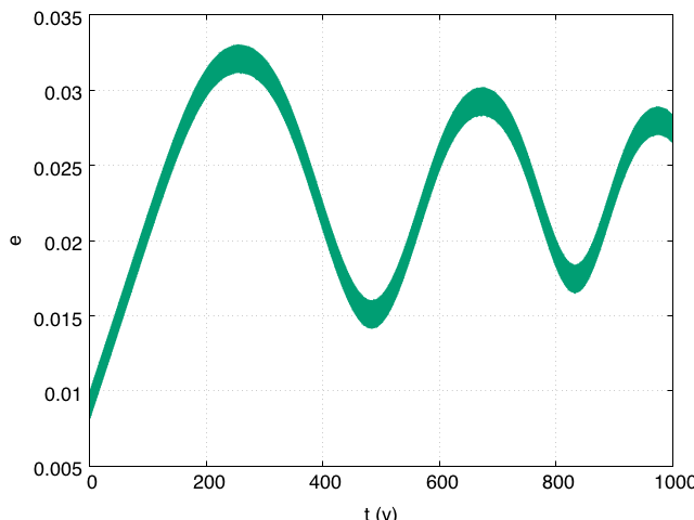
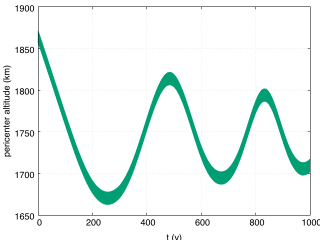
Figure 8: On the left, eccentricity evolution computed with FOP for $A/m=0.012$ m${}^{2}/$kg, starting from $a=r_{\bigoplus}+1940$ km, $e=0.01$, $i=80^{\circ}$, $\Omega=90^{\circ}$, $\omega=90^{\circ}$ on June 21, 2020 at 06:43:12 (i.e., $\lambda_{S}\approx 90.086^{\circ}$). On the right, the consequent variation in pericenter altitude.

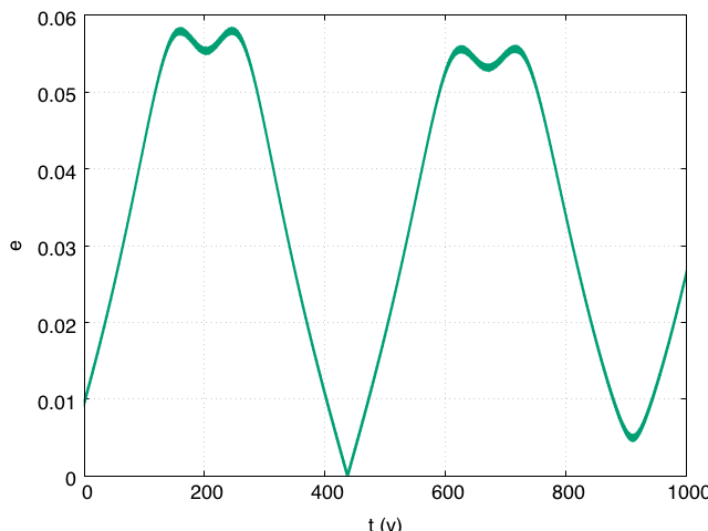
Figure 9: On the left, eccentricity evolution computed with FOP for $A/m=0.012$ m${}^{2}/$kg, starting from $a=r_{\bigoplus}+2600$ km, $e=0.01$, $i=36^{\circ}$, $\Omega=90^{\circ}$, $\omega=90^{\circ}$ on June 21, 2020 at 06:43:12 (i.e., $\lambda_{S}\approx 90.086^{\circ}$). On the right, the consequent variation in pericenter altitude.

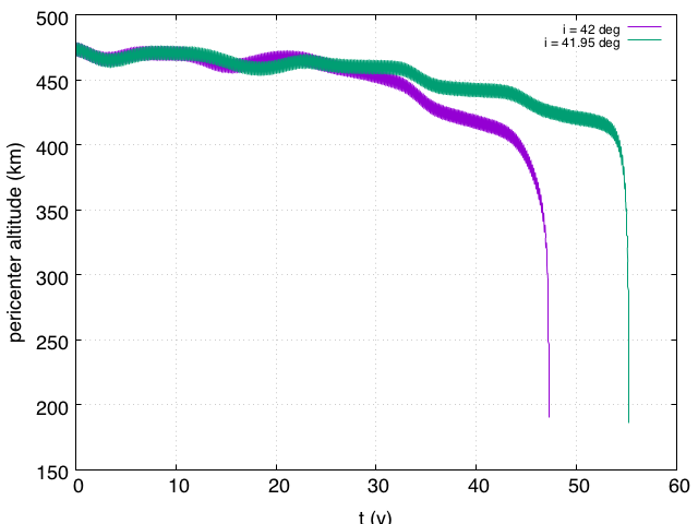
Figure 10: Pericenter altitude evolution computed with FOP for $A/m=0.012$ m${}^{2}/$kg, starting from $a=r_{\bigoplus}+840$ km, $e=0.05$, $i=42^{\circ}$ (purple) and $i=41.95^{\circ}$ (green), $\Omega=270^{\circ}$, $\omega=270^{\circ}$ on June 21, 2020 at 06:43:12 (i.e., $\lambda_{S}\approx 90.086^{\circ}$).

5 Conclusions

In this work, we have reviewed the main orbital resonances associated with solar radiation pressure which affects the evolution in eccentricity, in order to see if they might be exploited to design advantageous deorbiting solutions for Low Earth Orbits. Starting from a well-known theory, we have showed that at least four out of six resonances can be considered to increase the eccentricity of a small spacecraft equipped with a solar sail. The variation that can be achieved along a given resonance, that is, at well-defined values of semi-major axis, inclination and eccentricity, is such that a reentry to the Earth can be obtained, even from high altitudes. For typical values of operational satellites, SRP resonances can be considered, instead, in combination with the atmospheric drag, provided an accurate manoeuvring capability. The simplified model including only solar radiation pressure and Earth oblateness has been validated against a more realistic dynamical model. The corresponding results turn out to be consistent. The novelty of the work regards the possible applications, but it is also theoretical, because we have shown the importance of resonances which were neglected in the past.

Future work will look into the role of the initial phasing provided by initial epoch, longitude of ascending node and argument of pericenter, which could ensure either an increase or an eccentricity decrease. A detailed analysis on the characteristic frequencies for the eccentricity evolution in the resonant regions due to SRP is ongoing. That study will include also a comparison between the theoretical derivation explained here and the numerical results, without the contribution of the drag. Part of the results can be found in Schettino et al. (2017). Also, the inclination evolution was neglected in the analysis presented, and it will be evaluated in detail. From the point of view of a space operator, the model is still simplified in the sense that the orientation of a sail cannot be assumed as always directed normal to the solar radiation. This is another issue, which will deserve further research.

References

- Alessi et al. (2016) Alessi E. M., Deleflie F., Rosengren A. J., Rossi A., Valsecchi G. B., Daquin, J., Merz, K., 2016, Celestial Mechanics and Dynamical Astronomy, 125, 71
- Alessi et al. (2017a) Alessi E. M., Schettino G., Rossi A., Valsecchi G. B., 2017a, LEO Mapping for Passive Dynamical Disposal, Proceedings of the 7th European Conferences on Space Debris, Darmstadt, Germany
- Alessi et al. (2017b) Alessi E. M., Schettino G., Rossi A., Valsecchi G. B., 2017b, Dynamical Mapping of the LEO Region for Passive Disposal Design, 2017, International Astronautical Congress IAC-2017, paper IAC-17.A6.2.7
- Anselmo et al. (1996) Anselmo L., Cordelli A., Farinella P., Pardini C., Rossi A., 1996, Study on long term evolution of Earth orbiting debris, ESA/ESOC contract No. 10034/92/D/IM(SC)
- Beutler (2005) Beutler G., 2005, Methods of Celestial Mechanics II: Application to Planetary System, Geodynamics and Satellite Geodesy, Springer-Verlag, Berlin Heidelberg
- Breiter (1999) Breiter S., 1999, Celestial Mechanics and Dynamical Astronomy, 74, 253
- Brouwer & Clemence (1961) Brouwer D., Clemence G M., 1961, Methods of Celestial Mechanics, Academic Press, New York
- Casanova et al. (2015) Casanova D., Petit A., Lemaître A., 2015, Celestial Mechanics and Dynamical Astronomy, 123, 223
- Celletti et al. (2017) Celletti A., Efthymiopoulos C., Gachet F., Galeş C., 2017, International Journal of Non-Linear Mechanics, 90, 147
- Colombo et al. (2012) Colombo C., Lücking C., McInnes C. R., 2012, Acta Astronautica, 81, 137
- Colombo & McInnes (2012) Colombo C., McInnes C. R., 2012, International Astronautical Congress IAC-2012, paper IAC-12-C1.4.12
- Colombo & de Bras de Fer (2016) Colombo C., de Bras de Fer T., 2016, International Astronautical Congress IAC-2016, paper IAC-16-A6.4.4
- Colombo et al. (2017) Colombo C., Rossi A., Dalla Vedova F., 2017, International Astronautical Congress IAC-2017, paper IAC-17.A6.2.8
- Cook (1962) Cook G. E., 1962, The Geophysical Journal of the Royal Astronomical Society, 6, 271
- Daquin et al. (2016) Daquin J., Rosengren A. J., Alessi E. M., F. Deleflie, G. B. Valsecchi, Rossi A., 2016, Celestial Mechanics and Dynamical Astronomy, 124, 335
- Frouard et al. (2010) Frouard J., Fouchard M., Vienne A., 2010, A&A, 515, A54
- Hughes (1977) Hughes S., 1977, Planetary and Space Science, 25, 809
- Hughes (1980) Hughes S., 1980, Proceedings of the Royal Society of London. Series A, Mathematical and Physical Sciences, 372, 243
- Hughes (1981) Hughes S., 1981, Proceedings of the Royal Society of London. Series A, Mathematical and Physical Sciences, 375, 379
- Krivov et al. (1996) Krivov A. V., Sokolov L. L., Dikarev V. V., 1996, Celestial Mechanics and Dynamical Astronomy, 63, 313
- Lantukh et al. (2015) Lantukh D., Russell R. P., Broschart S., 2015, Celestial Mechanics and Dynamical Astronomy, 121, 171
- Lücking et al. (2012) Lücking C., Colombo C., McInnes C. R., 2012, Acta Astronautica, 77, 197
- Milani et al. (1987) Milani A., Nobili A., Farinella P., 1987, Non gravitational perturbations and satellite geodesy, Adam Hilger Ltd., Bristol and Boston
- Musen (1960) Musen P., 1960, Journal of Geophysical Research, 65, 1391
- Rosengren & Scheeres (2013) Rosengren A. J., Scheeres D. J., 2013, Advances in Space Research, 52, 1545
- Rosengren et al. (2015) Rosengren A., Alessi E. M., Rossi A., Valsecchi G. B., 2015, Monthly Notices of the Royal Astronomical Society, 449, 3522
- Rossi et al. (2009) Rossi A., Anselmo L., Pardini, C. Jehn, R., Valsecchi, G. B., 2009, The new space debris mitigation (SDM 4.0) long term evolution code, Proceedings of the Fifth European Conference on Space Debris, Darmstadt, Germany, Paper ESA SP-672
- Rossi et al. (2017) Rossi A., and the ReDSHIFT team, 2017, The H2020 Project ReDSHIFT: Overview, First Results and Perspectives, Proceedings of the 7th European Conference on Space Debris, Darmstadt, Germany
- Roy (1982) Roy A. E., 1982, Orbital Motion, Adam Hilger Ltd., Bristol
- Schettino et al. (2017) Schettino G., Alessi E. M., Rossi A., Valsecchi G. B., 2017, International Astronautical Congress, paper IAC-17.C1.9.2.
- Touma & Widsom (1998) Touma J., Wisdom J., 1998, The Astronomical Journal, 115, 1653
- Valk et al. (2007) Valk S., Lemaître A., Anselmo L., 2007, Advances in Space Research, 41, 1077