Kinetic models for goods exchange in a multi-agent market

Abstract

In this paper we introduce a system of kinetic equations describing an exchange market consisting of two populations of agents (dealers and speculators) expressing the same preferences for two goods, but applying different strategies in their exchanges. Similarly to the model proposed in TBD , we describe the trading of the goods by means of some fundamental rules in price theory, in particular by using Cobb-Douglas utility functions for the exchange. The strategy of the speculators is to recover maximal utility from the trade by suitably acting on the percentage of goods which are exchanged. This microscopic description leads to a system of linear Boltzmann-type equations for the probability distributions of the goods on the two populations, in which the post-interaction variables depend from the pre-interaction ones in terms of the mean quantities of the goods present in the market. In this case, it is shown analytically that the strategy of the speculators can drive the price of the two goods towards a zone in which there is a marked utility for their group. Also, according to TBD , the general system of nonlinear kinetic equations of Boltzmann type for the probability distributions of the goods on the two populations is described in details. Numerical experiments then show how the policy of speculators can modify the final price of goods in this nonlinear setting.

I Introduction

In recent years, there has been an increasing interest in developing kinetic models able to describe price formation in a multi-agent society, by resorting to methods typical of statistical mechanics NPT ; PT13 . In CPP Cordier, Pareschi and Piatecki introduce a kinetic description of the behavior of a simple financial market consisting of a population of agents where each agent can choose to invest between a stock and a bond. In this case, the variation of density is derived starting from the microscopic model for price formation introduced in LLS ; LLSb , usually known as Levy–Levy–Solomon model. The kinetic model proposed in CPP attempts to join to simple financial rules a kinetic equation of Boltzmann type, able to describe a complex behavior that could then mimic the market and explain the price formation mechanism.

A further example of coupling wealth with behavioral aspects has been proposed in MD . This research studies a relatively simple kinetic model for a financial market characterized by a single stock or good and an interplay between two different trader populations, chartists and fundamentalists, which determine the price dynamics of the stock. The model has been inspired by the microscopic Lux–Marchesi model LMa ; LMb . The financial rules depends here from the opinion of traders through a kinetic model of opinion formation recently introduced in To1 . A related model has been developed in BT , by allowing the opinion variable, which is mainly responsible of the trading, to be strictly connected to price acceleration.

Also, the importance of the personal knowledge of agents has been recently investigated in PT15 , in order to outline how wealth inequality could depend on knowledge distribution in a population.

In a recent paper, driven by the assumption that people trades to improve its utility, we coupled the methods of statistical mechanics and kinetic theory with some principle of price theory in microeconomics TBD , considering binary interactions following the rule furnished by the Edgeworth box Edg , which is frequently used in general equilibrium theory. Edgeworth box can fruitfully be applied in presence of an agent-based system in which agents possess a finite number of goods of $n\geq 2$ different types. Inspired by this mechanism of increasing utility and competitive equilibrium, in TBD was introduced and studied a kinetic equation of Boltzmann type for the evolution of the distribution density of the quantities of two goods in a system of agents. The exchange rule based on the Edgeworth box idea leads to a highly nonlinear binary interaction, which is difficult to handle, if not numerically.

For this reason, in TBD was considered a suitable linear Boltzmann equation, obtained by allowing the agent to interact (according to Edgeworth box), simultaneously with a sufficiently high number of agents in the market. For this model, it was shown that this linear equation has a unique solution, and the steady states are concentrated along a well-defined line (the price line).

Motivated by the interesting outcomes of the kinetic model based on binary trades driven by the Edgeworth box exchange, and taking into account the intrinsic interest of studying different types of populations which behave differently with the aim of getting maximum utility MD ; LMa ; LMb ; PT15 , in what follows we will introduce and discuss a kinetic description of a multi-agent system composed by two populations which interact according to the principle to get maximum utility, but allowing one of the two populations to exchange goods, by using only a part of them in the cross exchange, with the aim of getting a better profit from this strategy. In analogy with Lux-Marchesi description LMa ; LMb we will define this population as the population of speculators, by leaving the name of dealers to the other one.

Applying simple principles of micro–economy SST , we first derive in Section III a linear system of kinetic equations of Boltzmann type, which describes the evolution of the quantities of goods in the two populations. It is shown that the evolution in time of the mean price obeys a non linear law, which in some cases can be explicitly given, to show that the speculators can effectively obtain a net wealth gain from their strategy. Then, in Section IV we will introduce a system of nonlinear kinetic equations, similar to the one considered in TBD , which is able do describe the action of a group of speculators in a market of dealers. Numerical experiments, performed in Section V, enlighten the possible outcomes of the various strategies.

II The basic model

As discussed in the introduction, most of the existing kinetic models for wealth distribution are based on rigid assumptions which, if on one hand can be shared, from the other hand are not deeply related to economic principles, like price theory Fri . The aim of this Section is to introduce a framework for trades, which is derived directly from the basic principles of economy SST (cf. also LLS ).

Individuals exchange goods. The benefits they receive depend on how much they exchange and on what terms. Price theory tries to give an answer to this fundamental question.

For simplicity, let us start by considering a market with a number $N$ of agents which possess goods of two different types, we denote by $X$ and $Y$. At the starting time, agents (indexed by $k$) possess certain amounts $x_{k}=x_{k}(0)$ of good $X$ and $y_{k}=y_{k}(0)$ of good $Y$. While it is clear that $x_{k}$ and $y_{k}$ belong to $\mathbb{N}_{+}$, to avoid inessential difficulties, and without loss of generality, we will always consider these numbers as positive real numbers. The total number of each good in the disposal of agents is given by

$$\sum_{k=1}^{N}x_{k}=M_{x},\quad\sum_{k=1}^{N}y_{k}=M_{y}.$$ (2.1)

We assume moreover that the marked is closed, so that the total quantity of goods to be exchanged remains fixed in time. At fixed intervals of time of length $\Delta t$, agents exchange parts of their goods following a certain strategy. In view of these exchanges, agents hold at times $t$ amounts of good $X$ and $Y$, respectively denoted by $x_{k}(t)$ and $y_{k}(t)$. By virtue of (2.1), for each time $t\geq\Delta t$

$$\sum_{k=1}^{N}x_{k}(t)=M_{x},\quad\sum_{k=1}^{N}y_{k}(t)=M_{y}.$$ (2.2)

By fixing the price in time of one of the two goods, say $X$, equal to unity, and denoting by $P(t)>0$ the price of the second good $Y$, at each time $t\geq\Delta t$ any agent has a wealth $w_{k}(t)$ given by

$$w_{k}(t)=x_{k}(t_{-})+P(t)y_{k}(t_{-}).$$ (2.3)

In (2.3) $t_{-}=t-\Delta t$ denotes the last exchange time. The same notation will be used in the rest of the paper. At any subsequent time, agents determine fractions of their wealths, say $x$, to allocate the good $X$, with the reminder allocated to the good $Y$. In order to give a meaning to the reasons of this trading, it is classical to assume that agent’s behavior is driven by a utility function. One of the most popular of these functions is the Cobb-Douglas utility function

$$U(x)=x^{\alpha}(w_{k}(t)-x)^{\beta},\quad\alpha+\beta=1.$$ (2.4)

Each agent will tend to maximize its utility by trading. The values $\alpha$ and $\beta$ are linked to the preferences that the agent assigns to the two goods. If $\alpha>\beta$, the agent prefers to possess goods of the first type (numbered by $x$). The choice $\alpha=\beta=1/2$ clearly means that the two goods are equally important for $A$. The maximization of (2.4) updates the quantities of goods to

$$x_{k}(t)=\alpha w_{k}(t);\quad P(t)y_{k}(t)=\beta w_{k}(t).$$ (2.5)

The value of the unknown price $P(t)$ can be easily determined from the values of the variables at time $t-\Delta t$ by resorting to the constraint (2.2). Indeed it holds

$$\sum_{k=1}^{N}\alpha w_{k}(t)=M_{x};\quad\sum_{k=1}^{N}\beta w_{k}(t)=P_{k}(t)M_{y}.$$ (2.6)

Hence, solving for $P(t)$ we obtain the (fixed in time) price

$$P(t)=P=\frac{\beta M_{x}}{\alpha M_{y}}.$$ (2.7)

As expected, the (relative) price (2.7) of the good $Y$ is directly proportional to its preference value $\beta$, and inversely proportional to the quantity $M_{y}$ of goods of type $Y$ present in the closed marked. Substituting the expression for $P(t)$ back into (2.5) leads to the new quantities of goods

$$x_{k}(t)=x_{k}(t_{-})+\beta\left(\frac{M_{x}}{M_{y}}y_{k}(t_{-})-x_{k}(t_{-})\right)$$ (2.8)

$$y_{k}(t)=y_{k}(t_{-})+\alpha\left(\frac{M_{y}}{M_{x}}x_{k}(t_{-})-y_{k}(t_{-})\right).$$

This very simple mechanism of exchange can be easily generalized to different groups of traders, which can adopt different strategies. The simplest of these generalizations is to consider a market composed by two groups of agents, say $A$ and $B$, with fixed numbers $N_{A}$ and $N_{B}$ of agents belonging to the groups $A$ and $B$. As in the previous case, agents of both groups possess goods of two different types $X$ and $Y$. At the starting time, agents of the group $A$ possess certain amounts $x_{k}=x_{k}(0)$ of good $X$ and $y_{k}=y_{k}(0)$ of good $Y$, and the total number of each good in the disposal of agents of group $A$ is given by

$$\sum_{k=1}^{N_{A}}x_{k}=M_{x},\quad\sum_{k=1}^{N_{A}}y_{k}=M_{y}.$$ (2.9)

Likewise, agents of the group $B$ possess certain amounts $\tilde{x}_{k}=\tilde{x}_{k}(0)$ of good $X$ and $\tilde{y}_{k}=\tilde{y}_{k}(0)$ of good $Y$, and the total number of each good in the disposal of agents of group $B$ is given by

$$\sum_{k=1}^{N_{B}}\tilde{x}_{k}=m_{x},\quad\sum_{k=1}^{N_{B}}\tilde{y}_{k}=m_{y}.$$ (2.10)

By assuming that the marked is closed, the total quantity of goods at disposal of the two groups is conserved in time. However, since agents of the two groups interact on the same market, the total number of goods in each population can change with time. Therefore at time $t\geq\Delta t$

$$\sum_{k=1}^{N_{A}}x_{k}(t)=M_{x}(t),\quad\sum_{k=1}^{N_{A}}y_{k}(t)=M_{y}(t),$$ (2.11)

and

$$\sum_{k=1}^{N_{B}}\tilde{x}_{k}(t)=m_{x}(t),\quad\sum_{k=1}^{N_{B}}\tilde{y}_{k}=m_{y}(t).$$ (2.12)

The conservation of goods of type $X$ and $Y$ then implies

$$M_{x}(t)+m_{x}(t)=M_{x}+m_{x},\quad M_{y}(t)+m_{y}(t)=M_{y}+m_{y}$$ (2.13)

at any subsequent time $t\geq\Delta t$. At integer times $t\geq\Delta t$, agents of exchange parts of their goods. Agents of group $A$, the dealers, follows the previous strategy. Agents of group $B$, the speculators, follows a different strategy, essentially based on saving. While possessing amounts $(\tilde{x}_{k}(t_{-}),\tilde{y}_{k}(t_{-}))$ of goods, they exchange on the market only a part $(\lambda_{x}\tilde{x}_{k}(t_{-}),\lambda_{y}\tilde{y}_{k}(t_{-}))$ of their goods, where $0<\lambda_{x},\lambda_{y}<1$ are fixed constants. Consequently, the wealth of the $k$-th speculator, say $\tilde{w}_{k}(t)$ involved in the exchange is

$$\tilde{w}_{k}(t)=\lambda_{x}x_{k}(t_{-})+P(t)\lambda_{y}y_{k}(t_{-}).$$ (2.14)

Hence, in presence of this saving policy, the total quantity of goods to be exchanged does not coincide with the total (fixed) number of goods available in the market, given by the sum of the quantities (2.9) and (2.10). The saving policy of speculators introduces the (time dependent) constraints

$$\sum_{k=1}^{N_{A}}\alpha w_{k}(t)+\sum_{k=1}^{N_{B}}\alpha\tilde{w}_{k}(t)=M_{x}(t_{-})+\lambda_{x}m_{x}(t_{-}),$$ (2.15)

$$\sum_{k=1}^{N_{A}}\beta w_{k}(t)+\sum_{k=1}^{N_{B}}\beta\tilde{w}_{k}(t)=P(t)(M_{y}(t_{-})+\lambda_{y}m_{y}(t_{-})),$$

that express the effective quantities of goods present in the market at time $t-1$. Proceeding as before, agents of group $A$ update their goods as in (2.5). However, using the new constraints (LABEL:n-con) gives the time-dependent price

$$P(t)=\frac{\beta(M_{x}(t_{-})+\lambda_{x}m_{x}(t_{-}))}{\alpha(M_{y}(t_{-})+\lambda_{y}m_{y}(t_{-}))}.$$ (2.16)

Substituting the expression for $P(t)$ back into (2.3) leads for dealers to the new quantities of goods

$$x_{k}(t)= x_{k}(t_{-})+$$ (2.17)

$$+ \beta\left(\frac{M_{x}(t_{-})+\lambda_{x}m_{x}(t_{-})}{M_{y}(t_{-})+\lambda_{y}m_{y}(t_{-})}y_{k}(t_{-})-x_{k}(t_{-})\right)$$

$$y_{k}(t)= y_{k}(t_{-})+$$

$$+ \alpha\left(\frac{M_{y}(t_{-})+\lambda_{y}m_{y}(t_{-})}{M_{x}(t_{-})+\lambda_{x}m_{x}(t_{-})}x_{k}(t_{-})-y_{k}(t_{-})\right).$$

Likewise, speculators update their quantities of goods by

$$\tilde{x}_{k}(t)= \tilde{x}_{k}(t_{-})+$$ (2.18)

$$+ \beta\left(\frac{M_{x}(t_{-})+\lambda_{x}m_{x}(t_{-})}{M_{y}(t_{-})+\lambda_{y}m_{y}(t_{-})}\lambda_{y}\tilde{y}_{k}(t_{-})-\lambda_{x}\tilde{x}_{k}(t_{-})\right)$$

$$\tilde{y}_{k}(t)= \tilde{y}_{k}(t_{-})+$$

$$+ \alpha\left(\frac{M_{y}(t_{-})+\lambda_{y}m_{y}(t_{-})}{M_{x}(t_{-})+\lambda_{x}m_{x}(t_{-})}\lambda_{x}\tilde{x}_{k}(t_{-})-\lambda_{y}\tilde{y}_{k}(t_{-})\right).$$

Similar expressions for the updated quantities of goods have been obtained in TBD by resorting to the binary exchange rule provided by the Hedgeworth box, and subsequently linearizing the outcome. We will be back to this analogy later on.

III A Boltzmann system for trading of goods

III.1 The kinetic model

The previous model will be now modelled within the principles of statistical mechanics. Let the multi-agent system under study be composed by the two classes of agents of section II. Let $f(x,y,t)$ denote the density of agents of the class A (the dealers) with quantities $x$ and $y$ of the two goods at time $t\geq 0$, and let $g(x,y,t)$ denote the density of agents of the class $B$ (the speculators) with quantities $x$ and $y$ of the two goods at time $t\geq 0$. As before, and without loss of generality, we will assume that $x$ and $y$ are nonnegative real numbers. A system of Boltzmann-like equations of Maxwell type for the time evolution of the two densities $f(x,y,t)$ and $g(x,y,t)$ can be written in terms of the updated quantities (2.17) and (2.18) according to the following assumptions. The total number of each good in the disposal of agents at time $t\geq 0$, previously given by (2.11) and (2.12) is here substituted by the mean values of the density functions at time $t\geq 0$

$$M_{x}(t)=\int_{\mathbb{R}_{+}}x\,f(x,y,t)\,dx\,dy,$$ (3.19)

$$M_{y}(t)=\int_{\mathbb{R}_{+}}y\,f(x,y,t)\,dx\,dy,$$

and

$$m_{x}(t)=\int_{\mathbb{R}_{+}}x\,g(x,y,t)\,dx\,dy,$$ (3.20)

$$m_{y}(t)=\int_{\mathbb{R}_{+}}y\,g(x,y,t)\,dx\,dy.$$

We remark that this weaker assumption on the amount of goods effectively present in the market appears realistic, and it is consistent with the fact that agents in the market have an exact perception of the quantities of goods only in terms of their mean values. Moreover, to take into account that it is very difficult to exchange goods by performing an optimal exchange, we allow the updating of goods to be dependent of some randomness expressing deviation from the optimal choice, in any case by maintaining optimality in mean sense. In agreement with TBD this can be done by taking the values $0\leq\alpha(\omega)\leq 1$ and $0\leq\beta(\omega)\leq 1$ in the updated quantities (2.17) and (2.18) as positive independent random variables such that

$$\langle\alpha(\omega)\rangle=\alpha,\quad\langle\beta(\omega)\rangle=\beta,\quad\alpha+\beta=1,$$ (3.21)

where $\langle\cdot\rangle$ denotes mathematical expectation.

In reason of these choices, given a quantity $(x,y)$ of goods at time $t\geq 0$, the dealers will update their quantities according to

$$x^{*}=x+\beta(\omega)\left(\frac{M_{x}(t)+\lambda_{x}m_{x}(t)}{M_{y}(t)+\lambda_{y}m_{y}(t)}y-x\right)$$ (3.22)

$$y^{*}=y+\alpha(\omega)\left(\frac{M_{y}(t)+\lambda_{y}m_{y}(t)}{M_{x}(t)+\lambda_{x}m_{x}(t)}x-y\right).$$

Likewise, the speculators will update at time $t\geq 0$ the quantities $(x,y)$ according to

$$\tilde{x}^{*}=x+\beta(\omega)\left(\frac{M_{x}(t)+\lambda_{x}m_{x}(t)}{M_{y}(t)+\lambda_{y}m_{y}(t)}\lambda_{y}\,y-\lambda_{x}\,x\right)$$ (3.23)

$$\tilde{y}^{*}=y+\alpha(\omega)\left(\frac{M_{y}(t)+\lambda_{y}m_{y}(t)}{M_{x}(t)+\lambda_{x}m_{x}(t)}\lambda_{x}\,x-\lambda_{y}\,y\right).$$

Note that the law of variation of the goods in disposal at time $t>0$ depends on the mean values of the densities of the two groups at the same time.

In agreement with definition (2.16), the mean price $P(t)$ at time $t\geq 0$ of the second good relative to the first one is defined by

$$P(t)=\frac{\beta}{\alpha}\frac{M_{x}(t)+\lambda_{x}m_{x}(t)}{M_{y}(t)+\lambda_{y}m_{y}(t)}.$$ (3.24)

It is immediate to recognize that both interactions of type (LABEL:trA) and (LABEL:trB) imply the conservation in the mean, at each time $t\geq 0$, of the agent’s wealths. Indeed

$$w_{A}^{*}(t)= x^{*}+P(t)y^{*}=$$ (3.25)

$$x+P(t)y+\left(\beta(\omega)-\frac{\beta}{\alpha}\alpha(\omega)\right)\left(\frac{\alpha}{\beta}P(t)y-x\right),$$

$$\tilde{w}_{B}^{*}(t)= \tilde{x}^{*}+P(t)\tilde{y}^{*}=\tilde{x}+P(t)\tilde{y}\,+$$

$$+ \left(\beta(\omega)-\frac{\beta}{\alpha}\alpha(\omega)\right)\left(\frac{\alpha}{\beta}P(t)\lambda_{y}y-\lambda_{x}x\right),$$

which implies

$$\langle w_{A}^{*}(t)\rangle=x+P(t)y=w_{A}(t),$$ (3.26)

$$\langle\tilde{w}_{B}^{*}(t)\rangle=x+P(t)y=w_{B}(t).$$

Once the mechanism of variation of the quantities of goods has been defined, the evolution in time of the densities can be easily written down by expressing the law of variation in time of the observable quantities. It corresponds to write, for any given smooth function $\varphi$, a system of linear spatially homogeneous Boltzmann equations

$$\frac{d}{dt}\int_{\mathbb{R}_{+}^{2}}\varphi(x,y)f(x,y,t)\,dx\,dy=$$ (3.27)

$$\sigma\left\langle\int_{\mathbb{R}_{+}^{2}}(\varphi(x^{*},y^{*})-\varphi(x,y))f(x,y,t)\,dx\,dy\,\right\rangle,$$

$$\frac{d}{dt}\int_{\mathbb{R}_{+}^{2}}\varphi(x,y)g(x,y,t)\,dx\,dy=$$

$$\sigma\left\langle\int_{\mathbb{R}_{+}^{2}}(\varphi(\tilde{x}^{*},\tilde{y}^{*})-\varphi(x,y))g(x,y,t)\,dx\,dy\,\right\rangle.$$

In (LABEL:we) the positive constant $\sigma$ is a measure of the frequency of interactions. The right-hand sides of equations (LABEL:we) describe the change of density $f$ due the variation of type (LABEL:trA) (respectively the change of $g$ due the variation of type (LABEL:trB)). The two kinetic equations in (LABEL:we) are linked each other in view of the nature of the microscopic interactions, which involve the mean values of both densities. By choosing $\varphi(x,y)=x$ (respectively $\varphi(x,y)=y$) one reckons the laws of variation in time of the mean values (LABEL:ftotA) and (LABEL:ftotB) relative to the populations of dealers and speculators. The mean values of the population of dealers change according to

$$\frac{dM_{x}(t)}{dt}=\beta\left(\frac{M_{x}(t)+\lambda_{x}m_{x}(t)}{M_{y}(t)+\lambda_{y}m_{y}(t)}M_{y}(t)-M_{x}(t)\right),$$ (3.28)

$$\frac{dM_{y}(t)}{dt}=\alpha\left(\frac{M_{y}(t)+\lambda_{y}m_{y}(t)}{M_{x}(t)+\lambda_{x}m_{x}(t)}M_{x}(t)-M_{y}(t)\right).$$

Likewise, the mean values of the population of speculators change according to

$$\frac{dm_{x}(t)}{dt}=\beta\left(\frac{M_{x}(t)+\lambda_{x}m_{x}(t)}{M_{y}(t)+\lambda_{y}m_{y}(t)}\lambda_{y}m_{y}(t)-\lambda_{x}m_{x}(t)\right),$$ (3.29)

$$\frac{dm_{y}(t)}{dt}=\alpha\left(\frac{M_{y}(t)+\lambda_{y}m_{y}(t)}{M_{x}(t)+\lambda_{x}m_{x}(t)}\lambda_{x}m_{x}(t)-\lambda_{y}m_{y}(t)\right).$$

It is immediate to recognize that

$$M_{x}(t)+m_{x}(t)=I_{x}=M_{x}(0)+m_{x}(0),$$ (3.30)

$$M_{y}(t)+m_{y}(t)=I_{y}=M_{y}(0)+m_{y}(0).$$

These constraints reflect the conservation of the mean quantities of goods present in the closed market. Also, in view of (LABEL:con-ww) it holds

$$\frac{d}{dt}W_{A}(t)=M_{y}(t)\frac{d}{dt}P(t),$$ (3.31)

$$\frac{d}{dt}W_{B}(t)=m_{y}(t)\frac{d}{dt}P(t).$$

Equations (LABEL:evoW) express the time variation of the mean wealths of the agents of classes $A$ and $B$, in terms of the evolution of the price.

Remark III.1

It is interesting to remark that, provided that both the saving constants $\lambda_{x},\lambda_{y}$ are strictly positive, we have a further conservation law. Thanks to (LABEL:conXY)

$$M_{x}(t)+\lambda_{x}m_{x}(t)=I_{x}-(1-\lambda_{x})m_{x}(t),$$ (3.32)

$$M_{y}(t)+\lambda_{y}m_{y}(t)=I_{y}-(1-\lambda_{y})m_{y}(t).$$

A further conservation follows considering that, if for any given $r>0$

$$\Phi_{x}(r)=\frac{1}{\beta(1-\lambda_{x})}\log{\left[I_{x}-(1-\lambda_{x})r\right]},$$ (3.33)

it holds

$$-\frac{d\Phi_{x}(m_{x}(t))}{dt}=-\Phi_{x}^{\prime}(m_{x}(t))\frac{dm_{x}(t)}{dt}=$$ (3.34)

$$+\frac{1}{\beta\left[I_{x}-(1-\lambda_{x})m_{x}(t)\right]}\frac{dm_{x}(t)}{dt}=$$

$$\frac{\lambda_{y}m_{y}(t)}{I_{y}-(1-\lambda_{y})m_{y}(t)}-\frac{\lambda_{x}m_{x}(t)}{I_{x}-(1-\lambda_{x})m_{x}(t)}.$$

In analogous way, if

$$\Phi_{y}(r)=\frac{1}{\alpha(1-\lambda_{y})}\log{\left[I_{y}-(1-\lambda_{y})r\right]},$$ (3.35)

it holds

$$-\frac{d\Phi_{y}(m_{y}(t))}{dt}=\frac{\lambda_{x}m_{x}(t)}{I_{x}-(1-\lambda_{x})m_{x}(t)}-\frac{\lambda_{y}m_{y}(t)}{I_{y}-(1-\lambda_{y})m_{y}(t)}$$ (3.36)

Consequently

$$\frac{d\left[\Phi_{x}(m_{x}(t))+\Phi_{y}(m_{y}(t))\right]}{dt}=0,$$

which implies the conservation law

$$\left(I_{x}-(1-\lambda_{x})m_{x}(t)\right)^{1/[\beta(1-\lambda_{x})]}\cdot$$ (3.37)

$$\cdot\left(I_{y}-(1-\lambda_{y})m_{y}(t)\right)^{1/[\alpha(1-\lambda_{y})]}=C_{0},$$

Since the laws of evolution (LABEL:meA) and (LABEL:meB) are nonlinear, even in presence of conservation laws, a precise analytical study of systems (LABEL:meA) and (LABEL:meB) appears very difficult. Likewise, it is cumbersome to find the evolution of the higher moments of the solutions to (LABEL:we) in a closed form. Hence, the Boltmann equation (LABEL:we) is the starting point for a numerical study of the evolution of the densities by means of Monte Carlo methods BT ; Pa .

III.2 An explicitly solvable case

In what follows, we will discuss the situation in which the agents of the class $B$ will trade on the closed market only goods of one type, say $Y$, with the intent to increase their quantity of goods of type $X$. This corresponds to choose $\lambda_{x}=0$, and $\lambda_{y}=\delta$. The simplest case is obtained when $\lambda_{y}=1$, namely the case in which agents of the second class will exchange into the marked the total amount of their goods of type $Y$.

If this is the case, the second equation in (LABEL:meB) reduces to

$$\frac{dm_{y}(t)}{dt}=-\alpha m_{y}(t),$$ (3.38)

which can be easily solved to give

$$m_{y}(t)=m_{y}(0)\exp\{-\alpha t\}.$$ (3.39)

This shows that the goods of type $Y$ in the hands of the class $B$ of agents is exponentially decreasing in time at a rate proportional to $\alpha$, and the class $B$ will remain only with goods of type $Y$.

Then, owing to the conservations (LABEL:conXY) the first equation in (LABEL:meA) takes the form

$$\frac{dM_{x}(t)}{dt}= \beta\left(\frac{M_{x}(t)}{M_{y}(t)+m_{y}(t)}M_{y}(t)-M_{x}(t)\right)=$$ (3.40)

$$- \beta M_{x}(t)\frac{m_{y}(t)}{I_{y}}.$$

Hence we have

$$\frac{d\log M_{x}(t)}{dt}=-\beta\frac{m_{y}(0)}{I_{y}}\exp\{-\alpha t\},$$ (3.41)

that can be integrated to give

$$M_{x}(t)=M_{x}(0)\exp\left\{-\frac{\beta}{\alpha}\frac{m_{y}(0)}{I_{y}}\left(1-\exp\{-\alpha t\}\right)\right\}.$$ (3.42)

As expected, the quantity of goods of type $X$ in the class $A$ of agents is decreasing in time, and will exponentially reach the limit value

$$\bar{M}_{x}=M_{x}(0)\exp\left\{-\frac{\beta}{\alpha}\frac{m_{y}(0)}{I_{y}}\right\}.$$

Owing to the conservation laws (LABEL:conXY), from (3.39) and (3.42) we then obtain the values of $m_{x}(t)$ and $M_{y}(t)$. Also, the mean price $P(t)$ defined in (3.24) is

$$P(t)=\frac{\beta}{\alpha}\frac{M_{x}(0)}{I_{y}}\exp\left\{-\frac{\beta}{\alpha}\frac{m_{y}(0)}{I_{y}}\left(1-\exp\{-\alpha t\}\right)\right\}.$$ (3.43)

The price of the good $Y$ relative to $X$ is decreasing in time, and it will reach the limit value

$$\bar{P}=\frac{\beta}{\alpha}\frac{M_{x}(0)}{I_{y}}\exp\left\{-\frac{\beta}{\alpha}\frac{m_{y}(0)}{I_{y}}\right\}.$$

Note that in this case the time variation of the wealths of the two classes, given by (LABEL:evoW) is negative, and both classes will show their wealths decrease in time.

Consider the case in which initially the two classes possess the same mean quantity of the good $Y$, but the class $A$ possesses a bigger mean quantity of the good $X$. Then, at time $t=0$ one has $W_{A}(0)>W_{B}(0)$. Since the class $B$ is transferring goods of type $Y$ to the class $A$, at any subsequent time $t>0$ the difference $M_{y}(t)-m_{y}(t)$ is positive, and the relative wealth $W_{A}(t)-W_{B}(t)$, in reason of (LABEL:evoW) is decreasing in time. In this case, the strategy of the agents of the class $B$ is such that its final wealth is closer to the wealth of the class $A$.

The previous example shows that the eventual strategy of the agents of the class $B$ is able to determine an effective improvement of their wealth conditions.

III.3 The general case

Let us set

$$\rho_{x}(t)=\frac{M_{x}(t)}{M_{x}(t)+\lambda_{x}m_{x}(t)},$$ (3.44)

$$\rho_{y}(t)=\frac{M_{y}(t)}{M_{y}(t)+\lambda_{y}m_{y}(t)}.$$

Then, equations (LABEL:meA) can be rewritten as

$$\frac{1}{M_{x}(t)+\lambda_{x}m_{x}(t)}\frac{dM_{x}(t)}{dt}=\beta\left(\rho_{y}(t)-\rho_{x}(t)\right),$$ (3.45)

$$\frac{1}{M_{y}(t)+\lambda_{y}m_{y}(t)}\frac{dM_{y}(t)}{dt}=\alpha\left(\rho_{x}(t)-\rho_{y}(t)\right).$$

Using the constraints (LABEL:conXY) it follows that

$$\frac{d\rho_{x}(t)}{dt}=\frac{\lambda_{x}I_{x}}{\left(\lambda_{x}I_{x}+(1-\lambda_{x})M_{x}(t)\right)^{2}}\frac{dM_{x}(t)}{dt},$$ (3.46)

and analogous result (changing $x$ with $y$) for $\rho_{y}(t)$. Hence, since (LABEL:def-rho) imply

$$\frac{\lambda_{x}I_{x}}{\lambda_{x}I_{x}+(1-\lambda_{x})M_{x}(t)}=1-(1-\lambda_{x})\rho_{x},$$ (3.47)

equations (LABEL:meAA) take the form

$$\frac{d\rho_{x}(t)}{dt}=\beta(1-(1-\lambda_{x})\rho_{x}(t))\left(\rho_{y}(t)-\rho_{x}(t)\right),$$ (3.48)

$$\frac{d\rho_{y}(t)}{dt}=\alpha(1-(1-\lambda_{y})\rho_{y}(t))\left(\rho_{x}(t)-\rho_{y}(t)\right).$$

It is clear that the equilibrium points of system (LABEL:meA-A) are obtained when $\rho_{x}=\rho_{y}$. on the other hand, the conservation law (LABEL:con6) implies that, in equilibrium the function

$$H(\rho_{x}(t),\rho_{y}(t))= \left((1-(1-\lambda_{x})\rho_{x}(t))\right)^{1/\beta(1-\lambda_{x})}\cdot$$ (3.49)

$$\left((1-(1-\lambda_{y})\rho_{x}(t))\right)^{1/\alpha(1-\lambda_{x})}$$

satisfies the identity

$$H(\rho_{x},\rho_{y})=H(\rho_{x},\rho_{x})=H(\bar{\rho}_{x},\bar{\rho}_{y}),$$ (3.50)

where $\bar{\rho}_{x},\bar{\rho}_{y}$ denote the initial values. Since the function $H=H(u,v)$ is decreasing with respect to both $u$ and $v$ when $0<u,v<1$, whenever $\bar{\rho}=\min\{\bar{\rho}_{x},\bar{\rho}_{y}\}$

$$H(\bar{\rho}_{x},\bar{\rho}_{y})\geq H(\bar{\rho},\bar{\rho}).$$

Hence, there is a unique equilibrium point $\rho$ with $\min\{\bar{\rho}_{x},\bar{\rho}_{y}\}\leq\rho\leq\max\{\bar{\rho}_{x},\bar{\rho}_{y}\}$ in which

$$H(\rho,\rho)=H(\bar{\rho}_{x},\bar{\rho}_{y}).$$

In correspondence to this equilibrium point, we obtain the limit value of the price

$$\bar{P}=\frac{\beta\lambda_{x}I_{x}}{\alpha\lambda_{y}I_{y}}\frac{1-(1-\lambda_{y})\rho}{1-(1-\lambda_{x})\rho}.$$ (3.51)

IV A system of nonlinear Boltzmann equations

The basic model discussed in Section III can be easily adapted to recover a microscopic binary interaction between agents of the same class, or between agents of different classes.

For simplicity, let us start as in Section II by considering a market with a number $N$ of agents which possess goods of two different types $X$ and $Y$. Consider now at time $t$ a trading between two agents with wealths $w_{j}(t)$ and $w_{k}(t)$ given respectively by

$$w_{j}(t)=x_{j}(t_{-})+P(t)y_{j}(t_{-}),$$ (4.52)

$$w_{k}(t)=x_{k}(t_{-})+P(t)y_{k}(t_{-}).$$

Then, both agents determine a fractions of their wealths to allocate the good $X$, with the reminder allocated to the good $Y$. Using again the Cobb-Douglas utility function (2.4) agents will update the quantities of goods to

$$x_{j}(t)=\alpha w_{j}(t),\quad P(t)y_{j}(t)=\beta w_{j}(t),$$ (4.53)

$$x_{k}(t)=\alpha w_{k}(t),\quad P(t)y_{k}(t)=\beta w_{k}(t).$$

At difference with the previous (global) analysis of the closed market, the value of the price $P(t)$ is now determined from the values of the variables at time $t-\Delta t$ by resorting to the constraints of conservation of the sums of goods of type $X$ and $Y$ of the two agents $j$ and $k$. In this case

$$\alpha(w_{j}(t)+w_{k}(t))=x_{j}(t_{-})+x_{k}(t_{-}),$$ (4.54)

$$\beta(w_{j}(t)+w_{k}(t))=P_{k}(t)(y_{j}(t_{-})+y_{k}(t_{-})).$$

Hence, solving for $P(t)$ we obtain the relation

$$P(t)=\frac{\beta}{\alpha}\frac{x_{j}(t_{-})+x_{k}(t_{-})}{y_{j}(t_{-})+y_{k}(t_{-})}.$$ (4.55)

Substituting the expression for $P(t)$ back into (2.5) leads for the agent $j$ to the new quantities of goods

$$x_{j}(t)=x_{j}(t_{-})+\beta\left(\frac{x_{j}(t_{-})+x_{k}(t_{-})}{y_{j}(t_{-})+y_{k}(t_{-})}y_{j}(t_{-})-x_{j}(t_{-})\right)$$ (4.56)

$$y_{j}(t)=y_{j}(t_{-})+\alpha\left(\frac{y_{j}(t_{-})+y_{k}(t_{-})}{x_{j}(t_{-})+x_{k}(t_{-})}x_{j}(t_{-})-y_{j}(t_{-})\right).$$

Analogous result holds for the updating of the quantities of goods of the agent $k$.

This binary exchange can be easily generalized to the two groups of dealers and speculators considered before. In a binary exchange between the dealer $j$ of the class $A$ and the speculator $k$ of the class $B$, the dealer $j$ updates its goods according to

$$x_{j}(t)=x_{j}(t_{-})+\beta\left(\frac{x_{j}(t_{-})+\lambda_{x}x_{k}(t_{-})}{y_{j}(t_{-})+\lambda_{y}y_{k}(t_{-})}y_{j}(t_{-})-x_{j}(t_{-})\right),$$ (4.57)

$$y_{j}(t)=y_{j}(t_{-})+\alpha\left(\frac{y_{j}(t_{-})+\lambda_{y}y_{k}(t_{-})}{x_{j}(t_{-})+\lambda_{x}x_{k}(t_{-})}x_{j}(t_{-})-y_{j}(t_{-})\right).$$

Likewise, a speculator $k$ updates its quantities of goods according to

$$x_{k}(t)= x_{k}(t_{-})+$$ (4.58)

$$+ \beta\left(\frac{x_{j}(t_{-})+\lambda_{x}x_{k}(t_{-})}{y_{j}(t_{-})+\lambda_{y}y_{k}(t_{-})}\lambda_{y}y_{k}(t_{-})-\lambda_{x}x_{k}(t_{-})\right),$$

$$y_{k}(t)= y_{k}(t_{-})+$$

$$+ \alpha\left(\frac{y_{j}(t_{-})+\lambda_{y}y_{k}(t_{-})}{x_{j}(t_{-})+\lambda_{x}x_{k}(t_{-})}\lambda_{k}x_{k}(t_{-})-\lambda_{y}y_{k}(t_{-})\right).$$

We remark that similar expressions for the updated quantities of goods have been obtained in TBD by resorting to the binary exchange rule provided by the Hedgeworth box. Similarly to the model considered of TBD we can use the binary exchanges (LABEL:n55) , (LABEL:n65) and (4.58) to construct a system of bilinear Boltzmann type equations.

We assume that the dealers can interact with other dealers, and with speculators, according to their respective rules (LABEL:n55) and (LABEL:n65), while speculators interact only with dealers, according to (4.58). As before, let $f(x,y,t)$ denote the density of dealers of the class $A$ with quantities $x$ and $y$ of the two goods at time $t\geq 0$, and let $g(x,y,t)$ denote the density of speculators of the class $B$ with quantities $x$ and $y$ of the two goods at time $t\geq 0$. Then $f(x,y,t)$ satisfies

$$\frac{d}{dt}\int_{\mathbb{R}_{+}^{2}}\varphi(x,y) f(x,y,t)\,dx\,dy=$$ (4.59)

$$\sigma\int_{\mathbb{R}_{+}^{2}}\varphi(x,y)Q(f,f)(x,y)\,dxdy+$$

$$+ \mu\int_{\mathbb{R}_{+}^{2}}\varphi(x,y)P(f,g)(x,y)\,dxdy.$$

The constants $\sigma$ and $\nu$ measure the frequency of collisions. The right-hand side of equation (LABEL:we) describes the change of density due to exchanges between dealers (the operator $Q$) and exchanges dealer–speculator (the operator $P$). The definitions of $Q$ and $P$ are fruitfully given by their action on observable quantities

$$\int_{\mathbb{R}_{+}^{2}}\varphi(x,y)Q(f,f)(x,y)\,dxdy=$$ (4.60)

$$\left\langle\int_{\mathbb{R}_{+}^{4}}(\varphi(x^{*},y^{*})-\varphi(x,y))f(x,y,t)f(x_{1},y_{1},t)\,d\pi\right\rangle,$$

where, now and later on, $d\pi=dx\,dy\,dx_{1}\,dy_{1}$, and

$$x^{*}=x+{\beta(\omega)}\left(\frac{x+x_{1}}{y+y_{1}}y-x\right),$$ (4.61)

$$y^{*}=y+{\alpha(\omega)}\left(\frac{y+y_{1}}{x+x_{1}}x-y\right).$$

Likewise

$$\int_{\mathbb{R}_{+}^{2}}\varphi(x,y)P(f,g)(x,y)\,dxdy=$$ (4.62)

$$\left\langle\int_{\mathbb{R}_{+}^{4}}\,(\varphi(\tilde{x},\tilde{y})-\varphi(x,y))f(x,y,t)g(x_{1},y_{1},t)\,d\pi\right\rangle,$$

where

$$\tilde{x}=x+{\beta(\omega)}\left(\frac{x+\lambda_{x}x_{1}}{y+\lambda_{y}y_{1}}y-x\right),$$ (4.63)

$$\tilde{y}=y+{\alpha(\omega)}\left(\frac{y+\lambda_{y}y_{1}}{x+\lambda_{x}x_{1}}x-y\right).$$

In agreement with Section III the values $0\leq\alpha(\omega)\leq 1$ and $0\leq\beta(\omega)\leq 1$ in (LABEL:AA) and (LABEL:AB) are positive independent random variables satisfying (3.21). Equation (4.59) is coupled with the evolution equation for $g(x,y,t)$, given by

$$\frac{d}{dt}\int_{\mathbb{R}_{+}^{2}}\varphi(x,y) f(x,y,t)\,dx\,dy=$$ (4.64)

$$\mu\int_{\mathbb{R}_{+}^{2}}\varphi(x,y)\bar{P}(g,f)(x,y)\,dxdy.$$

Clearly

$$\int_{\mathbb{R}_{+}^{2}}\varphi(x,y)\bar{P}(g,f)(x,y)\,dxdy=\left\langle\int_{\mathbb{R}_{+}^{4}}\,dx\,dy\,dx_{1}\,dy_{1}\right.$$ (4.65)

$$\left.(\varphi(\bar{x},\bar{y})-\varphi(x,y))g(x,y,t)f(x_{1},y_{1},t)\,\right\rangle,$$

where

$$\bar{x}=x+{\beta(\omega)}\left(\frac{x_{1}+\lambda_{x}x}{y_{1}+\lambda_{y}y}\lambda_{y}y-\lambda_{x}x\right),$$ (4.66)

$$\tilde{y}=y+{\alpha(\omega)}\left(\frac{y_{1}+\lambda_{y}y}{x_{1}+\lambda_{x}x}\lambda_{x}x-\lambda_{y}y\right).$$

Note that, denoting

$$x_{1}^{*}=x_{1}+{\beta(\omega)}\left(\frac{x+x_{1}}{y+y_{1}}y_{1}-x_{1}\right),$$ (4.67)

$$y_{1}^{*}=y_{1}+{\alpha(\omega)}\left(\frac{y+y_{1}}{x+x_{1}}x_{1}-y_{1}\right).$$

exchanging variables into the integral one has the identity

$$\left\langle\int_{\mathbb{R}_{+}^{4}}(x^{*}-x)f(x,y,t)f(x_{1},y_{1},t)\,d\pi\,\right\rangle=$$

$$\frac{1}{2}\left\langle\int_{\mathbb{R}_{+}^{4}}(x^{*}+x_{1}^{*}-x-x_{1})f(x,y,t)f(x_{1},y_{1},t)\,d\pi\,\right\rangle=0.$$

This property is not satisfied by the mixed operators $P(f.g)$ and $\bar{P}(g,f)$. However it can be easily verified that

$$\int_{\mathbb{R}_{+}^{2}}xP(f,g)(x,y)\,dxdy+\int_{\mathbb{R}_{+}^{2}}x\bar{P}(g,f)(x,y)\,dxdy=0.$$

The same properties hold if we substitute the good $x$ with the good $y$. This implies that the conservation of the mean values, as given by (LABEL:conXY) still hold for the nonlinear system . Since the exchanges of goods of type (LABEL:trB) are nonlinear, the study of the properties of the solution to the Boltzmann system appears difficult. The Boltmann system (4.59), (4.64) can however be studied from a numerical point of view.

V Numerical experiments

This section contains a numerical description of the solutions to the nonlinear Boltzmann system (4.59) and (4.64). For the numerical approximation of the Boltzmann equations we apply a Monte Carlo method, as described in Chapter 4 of PT13 . If not otherwise stated the kinetic simulation has been performed with $N=10^{4}$ agents.

The numerical experiments will help to clarify the effect of the strategy of speculators in the final distribution of the wealth density among the two classes of agents. It is evident from the experiments that, thanks to the conservations of the mean quantities of the goods, the densities $f(x,y,t)$ of dealers and $g(x,y,t)$ of speculators will converge to stationary distributions PT13 . As usual in kinetic theory, these stationary solutions will be reached in an exponentially fast time. We will evaluate the stationary solutions for different values of the parameters $\lambda_{x},\lambda_{y}$ and different values of the parameters $\alpha$ and $\beta$. In this way we will recognize first the effect of the strategy of speculators and, second, the role of the preferences parameters $\alpha$ and $\beta$ to reach the final distribution of wealth.

The main test represents a two-phases experiment. In the first phase, the convergence of the price to its equilibrium value is shown by considering only the population of dealers. Then, when the price is close to its equilibrium value, the speculators enter into the game to modify the price value. At difference with the linear model described in Section III, where in absence of the population of speculators the price of the goods in possess of the population of dealers takes a constant value, the nonlinear model exhibits oscillations in the price evolution, which reduce exponentially in time.

The test is intended to simulate the situation in which a small number of speculators are entering into the market to obtain a marked advantage in their wealth by a saving politics. Since the price of the goods is adapting exponentially fast in time, the experiment also justifies the fact that dealers have no time to adapt to the new situation by changing their preferences.

Figure 5.1: $\alpha=0.5;\beta=0.5;M_{x}=3;m_{x}=10;M_{y}=3;m_{y}=2;\lambda_{x}=0.8;\lambda_{y}=0.2$ (left); $\alpha=0.5;\beta=0.5;M_{x}=3;m_{x}=10;M_{y}=3;m_{y}=2;\lambda_{x}=0.5;\lambda_{y}=0.5$ (right).

The test is performed for different values of the relevant parameters $\alpha$, $\beta$, $\lambda_{x}$ and $\lambda_{y}$, to clarify their effect on the price evolution.

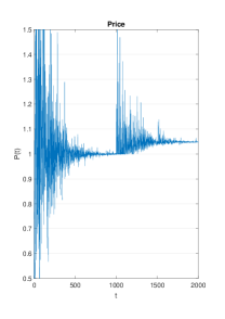
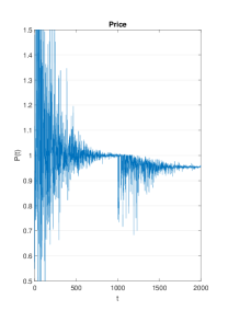
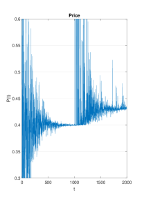
Figure 5.1 shows the variation of the (relative) price of the second good induced by the strategy of speculators. When the saving parameters $\lambda_{x}$ and $\lambda_{y}$ are such that $\lambda_{x}>\lambda_{y}$, the price of the good $Y$ is shown to increase (left). On the contrary, by taking the saving parameters equal, and by leaving the other quantities unchanged, the price of the good $Y$ is shown to increase (left). Note that in both cases the value of the price consequent to the action of the speculators decays exponentially fast towards the limit value.

Figure 5.2: $\alpha=0.25;\beta=0.75;M_{x}=3;m_{x}=10;M_{y}=3;m_{y}=2;\lambda_{x}=0.8;\lambda_{y}=0.2$ (left); $\alpha=0.75;\beta=0.25;M_{x}=3;m_{x}=10;M_{y}=3;m_{y}=2;\lambda_{x}=0.5;\lambda_{y}=0.5$ (right).

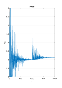
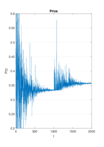
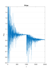
Figure 5.2 shows the variation of the (relative) price of the second good induced by the strategy of speculators in presence of a radical change of the preference parameters $\alpha$ and $\beta$. All the remaining parameters are left equal. While both experiments lead to a positive variation of the (relative) price of the second good, the final price in the two experiments is completely different. While in the case to the left, denoted by a marked preference for the good $Y$, the price of this good stabilizes around a value between $3$ and $3.5$, in the case to the right, characterized by a marked preference for the good $X$, the price of the good $y$ stabilizes around a value $0.35$, namely a factor ten below the prive of the experiment on the left.

Last, Figure 5.3 shows the evolution of price in the case of different choices of the saving parameters, coupled with different mean quantities of goods. As in the case of Figure 5.1 the relevant parameters which allow to increase (or decrease the final relative price of good $Y$ seem to be the saving parameters $\lambda_{x}$ and $\lambda_{y}$.

Figure 5.3: $\alpha=0.5;\beta=0.5;M_{x}=3;m_{x}=20;M_{y}=7,5;m_{y}=5;\lambda_{x}=0.8;\lambda_{y}=0.2$ (left); $\alpha=0.5;\beta=0.5;M_{x}=3;m_{x}=7.5;M_{y}=20;m_{y}=5;\lambda_{x}=0.2;\lambda_{y}=0.8$ (right).

VI Final remarks

In this paper we introduced two systems of kinetic equations of Boltzmann type suitable to describe the evolution of the probability distribution of two goods among two populations of agents, dealers and speculators, that apply different strategies in the exchanges. The leading idea was to describe the trading of these goods by means of some fundamental rules in prize theory, in particular by using Cobb-Douglas utility functions for the binary exchange. Also, to take into account the intrinsic risks of the market, we introduced randomness in the exchange, without affecting the microscopic conservations, that is the conservation of the total number of each good in the market.

Both the analytic study of the linear system (LABEL:we), and the numerical simulation of the nonlinear system (4.59) and (4.64) allow to conclude that the saving politics of the speculators is able to modify the final price of the goods, to achieve eventually a net gain.

References

• (1) G.Naldi, L.Pareschi, and G.Toscani Eds. Mathematical Modeling of Collective Behavior in Socio-Economic and Life Sciences, Birkhauser, Boston (2010).
• (2) L. Pareschi, and G. Toscani, Interacting Multiagent Systems: Kinetic Equations and Monte Carlo Methods, Oxford University Press, Oxford 2014.
• (3) S. Cordier, L. Pareschi, and C. Piatecki, J Stat Phys 134 161 (2009).
• (4) M. Levy, H. Levy, and S. Solomon, Econ. Lett. 45, 103 111 (1994).
• (5) M. Levy, H. Levy and S. Solomon, Microscopic Simulation of Financial Markets: From Investor Behaviour to Market Phenomena. Academic Press, San Diego (2000).
• (6) D. Maldarella, and L. Pareschi, Physica A, 391 715 (2012).
• (7) T. Lux, and M. Marchesi, International Journal of Theoretical and Applied Finance 3 675 (2000).
• (8) T. Lux, and M. Marchesi, Nature 397 (11) 498 (1999).
• (9) G. Toscani, Comm. in Math. Scie. 4 481 (2006).
• (10) C. Brugna, and G. Toscani, Netw. Heterog. Media 10 (3) 543 (2015).
• (11) L. Pareschi, and G. Toscani, Phil. Trans. R. Soc. A 372, 20130396, 6 October (2014).
• (12) G. Toscani, C. Brugna, and S. Demichelis, J. Statist. Phys, 151, 549 (2013).
• (13) F.Y. Edgeworth, Mathematical Psychics: An Essay on the Application of Mathematics to the Moral Sciences, Kegan Paul, London 1881.
• (14) J. Silver, E. Slud and K. Takamoto, J. Econ. The. 106 417 (2002).
• (15) D.D. Friedman, Price Theory: An Intermediate Text, South-Western Publishing Co. (1990).
• (16) L.Pareschi, and G.Russo, ESAIM: Proceedings, 10, 35 (2001).
• (17) J.A. Carrillo, S. Cordier, and G. Toscani, Discrete and Continuous Dynamical Systems A. 24 (1) 59 (2009).
• (18) B. Düring, D. Matthes, and G. Toscani, Phys. Rev. E 78, (2008) 056103.
• (19) D. Matthes, and G. Toscani, J. Stat. Phys. 130 1087 (2008).