An astrosphere around the blue supergiant $\kappa$ Cas: possible explanation of its filamentary structure

Abstract

High-resolution mid-infrared observations carried out by the Spitzer Space Telescope allowed one to resolve the fine structure of many astrospheres. In particular, they showed that the astrosphere around the B0.7 Ia star $\kappa$ Cas (HD 2905) has a clear-cut arc structure with numerous cirrus-like filaments beyond it. Previously, we suggested a physical mechanism for the formation of such filamentary structures. Namely, we showed theoretically that they might represent the non-monotonic spatial distribution of the interstellar dust in astrospheres (viewed as filaments) caused by interaction of the dust grains with the interstellar magnetic field disturbed in the astrosphere due to colliding of the stellar and interstellar winds. In this paper, we invoke this mechanism to explain the structure of the astrosphere around $\kappa$ Cas. We performed 3D magnetohydrodynamic modelling of the astrosphere for realistic parameters of the stellar wind and space velocity. The dust dynamics and the density distribution in the astrosphere were calculated in the framework of a kinetic model. It is found that the model results with the classical MRN size distribution of dust in the interstellar medium do not match the observations, and that the observed filamentary structure of the astrosphere can be reproduced only if the dust is composed mainly of big ($\mu$m-sized) grains. Comparison of the model results with observations allowed us to estimate parameters (number density and magnetic field strength) of the surrounding interstellar medium.

1 Introduction

Interaction of the stellar wind with the circum- and interstellar medium (ISM) results in the formation of structures called astrospheres. Severe interstellar extinction at low Galactic latitudes, where the majority of (massive) wind-blowing stars is concentrated, makes the infrared (IR) observations the most effective way for detection and study of astrospheres (e.g. van Buren, Noriega-Crespo & Dgani 1995). Nowadays, with the advent of the Spitzer Space Telescope, Wide-field Infrared Survey Explorer (WISE) and Herschel Space Observatory, many hundreds of new astrospheres were revealed (Peri et al. 2012; Cox et al. 2012; Kobulnicky et al. 2016). Some of them have a distinct filamentary (cirrus-like) structure (e.g. Gvaramadze et al. 2011a, b). Although the origin of this structure is not well understood, it seems likely that the regular interstellar magnetic field might play an important role in its formation (Gvaramadze et al. 2011b).

Recently, Katushkina et al. (2017; hereafter Paper I) presented a physical mechanism possibly responsible for the origin of the cirrus-like structure of astrospheres around runaway stars. It was shown that, under proper conditions, alternating minima and maxima of the dust density (seen like filaments) might appear between the astrospheric bow shock (BS) and the astropause (AP) because of periodical gyromotion of the dust grains around the interstellar magnetic field lines.

In the present work, we apply this mechanism to explain the morphology of the astrosphere around the runaway blue supergiant $\kappa$ Cas (HD 2905). We choose this particular astrosphere because of its distinct cirrus-like structure, as well as because the basic parameters of its associated star are known fairly well (see Section 2). In Section 3.1, we perform numerical modelling of interaction between the stellar wind and the magnetized ISM in the framework of a 3D magnetohydrodynamic (MHD) model. In Section 3.2, we present the kinetic modelling of the interstellar dust distribution in the wind-ISM interaction region. In Section 3.3, we post-process the simulations to make synthetic maps of infrared dust emission. In Section 4, we compare the model results with observations, estimate the interstellar plasma number density and magnetic field strength, and derive constraints on the dust parameters, required to better reproduce the observations. Summary and discussion are presented in Section 5.

2 Observational data

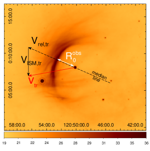
Figure 1: Spitzer MIPS 24 $\mu$m image of the astrosphere around the runaway blue supergiant $\kappa$ Cas. The dashed line shows the median line (or symmetry line) of the astrosphere. The red arrow shows the direction of transverse velocity of the star, $v_{\rm tr}$, as suggested by the Hipparcos proper motion measurement. Transverse components of the ISM velocity vector ($v_{\rm ISM,tr}$) and the vector of the star’s motion relative to the local ISM ($v_{\rm rel,tr}$) are shown as well (see text for details). The minimum (projected) separation between $\kappa$ Cas and the brightest arc in the astrosphere is marked as $R_{0}^{\rm obs}$. The colour bar shows the surface brightness on the linear scale in units of MJy sr^-1. The coordinates are the Galactic longitude and latitude on the horizontal and vertical scales, respectively. At a distance of 1 kpc, 1 arcmin corresponds to $\approx 0.29$ pc.

The astrosphere around the blue supergiant (B0.7 Ia; Walborn 1972) $\kappa$ Cas was discovered by van Buren & McCray (1988) using the Infrared Astronomical Satellite (IRAS) all-sky survey and presented for the first time in van Buren, Noriega-Crespo & Dgani (1995; see their fig. 2c). In the IRAS 60 $\mu$m image, the astrosphere has an arc-like shape, typical of bow shocks. The low resolution of the IRAS data, however, did not allow to see fine details of the astrosphere, which were revealed only with the advent of the Spitzer Space Telescope and the WISE mission with their much better angular resolution.

$\kappa$ Cas was observed by Spitzer on 2007 September 18 (Program Id.: 30088, PI: A.Noriega-Crespo) using the Multiband Imaging Photometer for Spitzer (MIPS; Rieke et al. 2004). We retrieved the post-basic data calibrated MIPS 24 $\mu$m image of $\kappa$ Cas (with units of MJy ${\rm sr}^{-1}$) from the NASA/IPAC infrared science archive. In this image (presented for the first time in Gvaramadze et al. 2011b) the astrosphere of $\kappa$ Cas appears (see Fig. 1) as a clear arcuate structure with numerous cirrus-like filaments beyond it, some of which are apparently attached to the main (brightest) arc. The surface brightness of this arc is $\approx$35 MJy ${\rm sr}^{-1}$, while that of the background is $\approx$20 MJy ${\rm sr}^{-1}$. Fig. 1 also shows several filaments intersecting the arc at almost right angle to its surface in the south part of the astrosphere. A possible origin of these filaments is discussed in Section 5.

We define the linear characteristic scale of the astrosphere as the minimum projected distance between $\kappa$ Cas and the brightest arc, $R_{0}^{\rm obs}$ (see Fig. 1), which is related to the observed angular separation between the star and the apex of the arc, $\Omega$, through the relationship $R_{0}^{\rm obs}=\Omega d$, where $d$ is the heliocentric distance to $\kappa$ Cas. For $\Omega=2.6$ arcmin and $d=1$ kpc (see below), one has $R_{0}^{\rm obs}\approx 0.75$ pc or $2.3\times 10^{18}$ cm.

It is believed that $\kappa$ Cas belongs to the Cas OB14 association, which is located at a distance of $d\approx 1.0\pm 0.1$ kpc (Humphreys 1978; Mel’nik & Dambis 2009). This distance is generally accepted in studies of $\kappa$ Cas (e.g. Crowther, Lennon & Walborn 2006; Searle et al. 2008). The presence of the astrosphere around $\kappa$ Cas, however, suggests that this star is a runaway and that it might be formed far away from its present position on the sky (cf. Gvaramadze, Pflamm-Altenburg & Kroupa 2011). Correspondingly, $\kappa$ Cas is not necessary a member of Cas OB14, unless this star has obtained its peculiar space velocity because of dissolution of a binary system in a recent supernova explosion in the association. In this connection, we note that among four members of the association listed in Humphreys (1978) one more star, HD 2619 (B0.5 III), produces a bow shock as well. The orientation of this bow shock (visible in WISE 22 and 12 $\mu$m images) suggests that HD 2619 was injected in Cas OB14 from the open star cluster Berkeley 59, located at a distance of $\approx 1$ kpc (Pandey et al. 2008) and at $\approx 3\aas@@fstack{\circ}5$ (or $\approx 60$  pc in projection) to the northwest from the star. It is possible therefore that Cas OB14 is actually a spurious association.

Table 1: Basic parameters of $\kappa$ Cas (Crowther et al. 2006; Searle et al. 2008).

$v_{\infty}$	$\dot{M}$	$T_{*}$	$R_{*}$	$\log(L_{*}/\rm\,L_{\odot})$
(${\rm\,km\,s^{-1}}$)	($\rm\,M_{\odot}\,{\rm yr}^{-1}$)	(kK)	($R_{\odot}$)
850$-$1000	$(2.0-2.5)\times 10^{-6}$	23.5	33	5.48

Table 2: Summary of astrometric and kinematic data on $\kappa$ Cas (see text for details).

$d$	$\mu_{\alpha}\cos\delta$	$\mu_{\delta}$	$v_{\rm r,hel}$	$v_{\rm l}$	$v_{\rm b}$	$v_{\rm r}$	$V_{\rm tr}$	$V_{*}$
(kpc)	(mas ${\rm yr}^{-1}$)	(mas ${\rm yr}^{-1}$)	(${\rm\,km\,s^{-1}}$)	(${\rm\,km\,s^{-1}}$)	(${\rm\,km\,s^{-1}}$)	(${\rm\,km\,s^{-1}}$)	(${\rm\,km\,s^{-1}}$)	(${\rm\,km\,s^{-1}}$)
1.0	3.65$\pm$0.17	$-$2.07$\pm$0.16	0.3$\pm$0.8	20.8$\pm$0.8	$-$3.8$\pm$0.8	18.5$\pm$0.8	21.1$\pm$1.1	28.1$\pm$1.4

A somewhat larger distance to $\kappa$ Cas follows from the Hipparcos parallax (van Leeuwen 2007) and the empirical relationship between the strength of the interstellar Ca ii lines and the distances to early-type stars (Megier et al. 2009), yielding respectively $d=1.37^{+0.42}_{-0.25}$ and $d=1.46\pm 0.30$ kpc. Taken at face value, these two distance estimates imply a too high bolometric luminosity of $\log(L_{*}/\rm\,L_{\odot})\approx 5.8$, which along with the effective temperature of $\kappa$ Cas of $T_{*}=23.5\pm 1.5$ kK (Searle et al. 2008) would place this star on the S Doradus instability strip (Wolf 1989) in the Hertzsprung-Russell diagram. Since $\kappa$ Cas does not show variability typical of stars in this region of the Hertzsprung-Russell diagram, it is likely that it is located at a shorter distance. In what follows, we adopt the distance to $\kappa$ Cas of d=1 kpc. The basic parameters of $\kappa$ Cas ($T_{*}$, $L_{*}$, stellar wind velocity $v_{\infty}$, mass loss rate $\dot{M}$ and radius $R_{*}$) are compiled in Table 1.

In Table 2 we provide astrometric and kinematic data on $\kappa$ Cas. The proper motion measurements, $\mu_{\alpha}\cos\delta$ and $\mu_{\delta}$, are based on the new reduction of the Hipparcos data by van Leeuwen (2007). The heliocentric radial velocity of the star, $v_{\rm r,hel}$, is taken from Gontcharov (2006). Using these data, the Solar galactocentric distance $R_{0}=8.0$ kpc and the circular Galactic rotation velocity $\Theta_{0}=240\,{\rm\,km\,s^{-1}}$ (Reid et al. 2009), and the solar peculiar motion $(U_{\odot},V_{\odot},W_{\odot})=(11.1,12.2,7.3)\,{\rm\,km\,s^{-1}}$ (Schönrich, Binney & Dehnen 2010), we calculated the peculiar transverse velocity $V_{\rm tr}=(v_{\rm l}^{2}+v_{\rm b}^{2})^{1/2}$, where $v_{\rm l}$ and $v_{\rm b}$ are, respectively, the velocity components along the Galactic longitude and latitude, the peculiar radial velocity $v_{\rm r}$, and the total space velocity $V_{*}$ of the star. For the error calculation, only the errors of the proper motion and the radial velocity measurements were considered. The obtained space velocity of $\approx 30\,{\rm\,km\,s^{-1}}$ implies that $\kappa$ Cas is a classical runaway star (e.g. Blaauw 1961).

The orientation of the symmetry axis of astrospheres around moving stars is determined by the orientation of the stellar velocity relative to the local ISM. In a static, homogeneous ISM and for a spherically-symmetric stellar wind, the symmetry axis of an astrosphere is aligned with the vector of stellar space motion. In this case, the geometry of detected astrospheres (bow shocks) can be used to infer the direction of stellar motion and thereby to determine possible parent clusters for the bow-shock-producing stars (e.g. Gvaramadze & Bomans 2008). In reality, however, the ISM might not necessary be at rest owing to the effects of nearby supernova explosions, expanding H ii  regions, or outflows from massive star clusters. Also, the shape of astrospheres of hot (runaway) stars might be affected by photoevaporation flows from nearby regions of enhanced density (cloudlets) caused by ultraviolet emission of these stars (e.g. Mackey et al. 2015; Gvaramadze et al. 2017).

Fig. 1 shows that the vector of the peculiar (transverse) velocity of $\kappa$ Cas is misaligned with the symmetry axis (median line) of the astrosphere by an angle $\alpha\approx 35\degr$. This misalignment might be caused by inaccuracy of the space velocity calculation or by the presence of a regular flow in the local ISM. We consider the latter possibility to be more likely because the Hipparcos proper motion measurement for $\kappa$ Cas is very reliable (see Table 2). We suggest, therefore, that the orientation of the astrosphere around $\kappa$ Cas is affected by a flow of the local ISM.

To reconcile the orientation of the astrosphere around $\kappa$ Cas with the orientation of the stellar transverse motion, one needs to assume that the ISM is moving in the north-south direction (i.e. almost along the Galactic longitude) with a transverse velocity of $V_{\rm ISM,tr}\approx 15\,{\rm\,km\,s^{-1}}$. In this case, the transverse component of the relative velocity between the star and the ISM is $V_{\rm rel,tr}\approx 26\,{\rm\,km\,s^{-1}}$. Allowing the possibility that the ISM could have a velocity component in the radial direction as large as in the transverse one, i.e. $\pm 15\,{\rm\,km\,s^{-1}}$, one finds that the total relative velocity, $V_{\rm rel}$, could range from 26 to $42\,{\rm\,km\,s^{-1}}$. For the sake of certainty, in our calculations we adopt an intermediate value of $V_{\rm rel}$ of $35\,{\rm\,km\,s^{-1}}$, which corresponds to the angle between the vector of the total relative velocity and the line of sight of $\theta=48\degr$. Note that the orientation of the astrosphere would not change if the transverse velocity of the ISM has a component in the east-west direction as well (i.e. parallel to the Galactic plane). The actual value of $V_{\rm rel}$ (or the sonic Mach number), however, is not critically important for our calculations because in the considered case (see below) the overall structure of the astrosphere is mostly determined by the interstellar magnetic field.

3 Numerical model

To compare the model astrospheres with observations one needs to produce synthetic maps of the thermal emission from the dust accumulated at the region of interaction between the stellar wind and the surrounding ISM. For this, the following steps should be performed: 1) MHD modelling of the plasma and magnetic field distributions in the astrosphere, 2) kinetic modelling of the interstellar dust distribution in the wind-ISM interaction region, and 3) determination of the dust temperature and calculation of the thermal emission intensity. These steps are presented in the next subsections.

3.1 3D MHD modelling of the astrosphere

To determine the distribution of plasma and magnetic field in and around the astrosphere we use the steady-state 3D MHD model described in Paper I. Here we also take into account the radiative cooling of plasma with the cooling function from Cowie et al. (1981). Note that the interstellar magnetic field is essential for this study due to two reasons. Firstly, the proposed physical mechanism for formation of filaments is based on gyrorotation of dust grains around magnetic field lines frozen into the interstellar plasma. Secondarily, in the absence of the magnetic field the radiative cooling strongly reduces the thickness of the layer between the AP and the BS because of loss of energy (see Fig. 2). Therefore, the filaments formed in this region would be unresolvable. In the presence of significant interstellar magnetic field the outer shock layer does not collapse (see Fig. 3) and the filaments might be observable.

Note that hereafter all distances in plots are dimensionless, they are normalized to the stand-off distance, which is the distance from the star to the AP in the upwind direction in the unmagnetized medium:

$$D^{*}=\sqrt{\frac{\dot{M}v_{\infty}}{4\pi\rho_{\rm p,ISM}V_{\rm rel}^{2}}},$$ (1)

where $\rho_{\rm p,ISM}=1.4n_{\rm p,ISM}\,m_{\rm p}$, $n_{\rm p,ISM}$ is the ISM number density of protons and $m_{\rm p}$ is the proton mass.

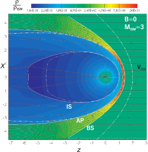
Figure 2: An axisymmetric model astrosphere in the ISM without magnetic field. The sonic Mach number is equal to 3. Solid and dot-dashed white curves show the positions of discontinuities (IS – inner shock, AP – astropause, BS – bow shock) for models with and without radiative cooling, respectively. The distribution of the plasma density in the model with cooling is colour-coded. Streamlines are shown by black lines.

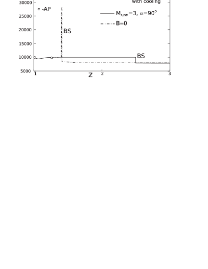
Figure 3: Plasma temperature distribution along the $Z$-axis (directed in the opposite direction to the ISM flow) outside of the astropause (AP) for model astrospheres with (solid lines) and without (dot-dashed lines) perpendicular magnetic field. In both models the radiative cooling is included and $M_{\rm ISM}$=3. BS stands for bow shock.

In the dimensionless form the solution of the problem depends on the sonic ($M_{\rm ISM}$) and Alfvenic ($M_{\rm A,ISM}$) Mach numbers of the ISM. In general, there is one more dimensionless parameter characterizing the efficiency of the radiative cooling. However, in the case of relatively high ISM number density ($n_{\rm p,ISM}\geq 2$ cm^-3, see Section 4) and for the adopted cooling function the plasma temperature in the outer shock region (i.e. between the AP and the BS) remains almost constant (see the solid curve in Fig. 3) and, correspondingly, the results do not depend on the dimensionless parameter related to the radiative cooling.

We perform calculations with the “perpendicular” interstellar magnetic field, i.e. with the magnetic field vector in the undisturbed ISM (${\bm{B}}_{\rm ISM}$) perpendicular to the relative ISM velocity vector (${\bm{V}}_{\rm ISM}=-{\bm{V}}_{\rm rel}$). We choose this orientation of the magnetic field because the nose part of the astrosphere around $\kappa$ Cas seems to be axisymmetric and because we know from Paper I that in the case of parallel magnetic field the dust is accumulated in filaments at flanks of the astrosphere and is absent in its nose part (see fig. 10 in Paper I). The effect of the stellar magnetic field is neglected in our calculations.

We assume that the ISM temperature is $\approx 7000-8000$ K, which along with $V_{\rm rel}=35\,{\rm\,km\,s^{-1}}$ (see Section 2) corresponds to the sonic Mach number of $M_{\rm ISM}\approx 3$. We performed calculations for several values of $M_{\rm A,ISM}$. The magnitude of the interstellar magnetic field (and Alfvenic Mach number) determines the thickness of the outer shock layer. It is found that the best qualitative agreement between the model results and the observations could be achieved for $M_{\rm A,ISM}\approx 1.5-3$ (see discussion in Section 5). The main part of the calculations presented in this work is performed for $M_{\rm A,ISM}=1.77$.

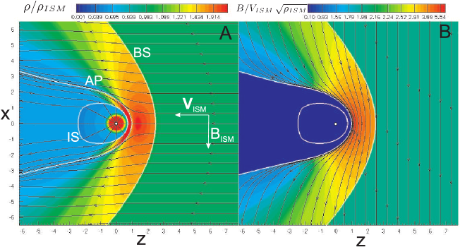
Figure 4: 2D distributions of the plasma density (panel A) and the magnetic field (panel B) in the $({\bm{V}}_{\rm ISM},{\bm{B}}_{\rm ISM})$-plane. The inner shock (IS), the astropause (AP) and the bow shock (BS) are plotted with white lines. The streamlines (panel A) and the magnetic field lines (panel B) are plotted with black lines.

Fig. 4 plots 2D distributions of the plasma density and the magnetic field in the $({\bm{V}}_{\rm ISM},{\bm{B}}_{\rm ISM})$-plane. Note that the thickness of the outer shock layer between the AP and the BS is determined by the chosen Alfvenic Mach number, i.e. the weaker the magnetic field (or the larger $M_{\rm A,ISM}$) the thinner the layer.

3.2 Kinetic modelling of the dust distribution in the astrosphere

To calculate the dust distribution in the astrosphere we use the kinetic model described in Alexashov et al. (2016) and Paper I. In general, the dynamics of charged interstellar dust grains in the astrosphere is determined by the following forces: the electromagnetic Lorentz force ${\bm{F}}_{\rm L}$, the stellar gravitational force ${\bm{F}}_{\rm G}$, the stellar radiation pressure ${\bm{F}}_{\rm rad}$, and the drag force ${\bm{F}}_{\rm drag}$ due to interaction of the dust grains with protons and electrons through the direct and Coulomb collisions. Therefore, the motion equation of a charged dust grain is the following:

$${{\rm d}{\bm{v}}_{\rm d}\over{\rm d}t}={q\over m_{d}c}({\bm{v}}_{\rm rel}\times{\bm{B}})+\left(-GM_{*}+{\sigma_{\rm d}\bar{Q}_{\rm rp}L_{*}\over 4\pi m_{d}c}\right){{\bm{e}}_{\rm r}\over r^{2}}$$

$$+\sigma_{\rm d}n_{\rm p}kT_{p}\hat{G}(v_{\rm rel},T_{p}){{\bm{v}}_{\rm rel}\over|{\bm{v}}_{\rm rel}|},$$ (2)

where $q$ and $m_{d}$ are the charge and mass of the grain, $c$ is the speed of light, ${\bm{v}}_{d}=\dot{{\bm{x}}}_{\rm d}$, ${\bm{x}}_{\rm d}$ is the position of a dust grain, $r=|{\bm{x}}_{\rm d}|$ is the distance from the star, ${\bm{e}}_{\rm r}$ is the unit vector in the radial direction, ${\bm{v}}_{\rm p}$ is the local plasma velocity, ${\bm{v}}_{\rm rel}={\bm{v}}_{\rm d}-{\bm{v}}_{\rm p}$ is the relative velocity between the plasma and the dust grain, ${\bm{B}}$ is the magnetic field, $G$ is the gravitational constant, $M_{*}$ and $L_{*}$ are the stellar mass and luminosity, $\sigma_{\rm d}=\pi r_{\rm d}^{2}$ is the geometrical cross section of the dust grain, $r_{\rm d}$ is the radius of the grain, $\bar{Q}_{\rm rp}\approx 1$ is the flux-weighted mean radiation pressure efficiency of the grain, $n_{\rm p}$ and $T_{p}$ are the plasma number density and temperature, $k$ is the Boltzmann constant, and $\hat{G}(v_{\rm rel},T)$ is the dimensionless function determining the drag force (see, e.g., Draine & Salpeter 1979; Ochsendorf et al. 2014). The plasma parameters ($n_{\rm p}$, ${\bm{v}}_{\rm p}$ and ${\bm{B}}$) are taken from the MHD model described above.

It is assumed that the dust grain charge $q$ is constant along the trajectory and $q=U_{\rm d,ISM}\,r_{\rm d}$, where $U_{\rm d,ISM}=+0.75$ V is the dust surface potential commonly assumed for the local ISM around the Sun (Grün & Svestka 1996). The potential is positive due to an influence of accretion of protons, photoelectric emission of stellar and interstellar radiation, and secondary electron emission (see, e.g. Kimura & Mann 1998; Akimkin et al. 2015).

We estimated the relative contribution of the listed forces to the dust dynamics in an astrosphere of $\kappa$ Cas and found that the stellar gravitation attractive force and the drag force are negligible compared with others. Stellar radiation force is especially important for small dust grains with radii $r_{\rm d}\leq 0.1\,\mu$m. These dust grains are swept out far away by the stellar radiation and do not cross the BS. Therefore, in our calculations we consider the dust grains with $r_{\rm d}>0.2\,\mu$m.

Classical power-law MRN size distribution (Mathis, Rumpl & Nordsieck, 1977) is assumed for the dust grains in the undisturbed ISM, $n_{\rm d,ISM}(r_{\rm d})\sim r_{\rm d}^{-3.5}$, with the minimum and maximum dust grain radii of 0.2 and $3\,\mu$m, respectively. Corresponding mass of the dust grains ranges from $8.37\times 10^{-14}$ to $2.83\times 10^{-10}$ g (it is assumed that the dust grains are spherical and have a uniform density $\rho_{\rm d}=2.5\,{\rm g}\,{\rm cm}^{-3}$). It is also assumed that in the undisturbed ISM all dust grains have the same velocity of ${\bm{V}}_{\rm ISM}$. The kinetic equation (2) is solved by the imitative Monte-Carlo method.

Fig. 5 plots the distribution of the dust number density in the (${\bm{B}}_{\rm ISM},{\bm{V}}_{\rm ISM})$-plane for dust grains with $r_{\rm d}=1\,\mu$m and $2\,\mu$m. In both cases, the filaments are clearly seen. Their formation is caused by periodical gyrorotation of charged dust grains around the magnetic field lines. This physical mechanism is extensively discussed in Paper I. The filaments produced by larger dust grains are sparser because of the larger gyroradius. It is shown in Paper I that the characteristic separation between filaments is:

$$D_{\rm gyr}=v_{{\rm p},z}\frac{2\pi m_{d}}{Bq}=v_{{\rm p},z}\frac{8\pi^{2}\rho_{\rm d}}{3}\frac{r_{\rm d}^{2}}{B\,U_{\rm{d,ISM}}},$$ (3)

where $v_{{\rm p},z}$ is the component of the plasma velocity along the $Z$-axis. For small $D_{\rm gyr}$ the filaments merge with each other and cannot be resolved. For the chosen model parameters ($M_{\rm A,ISM}$, $M_{\rm ISM}$, $\rho_{\rm d}$ and $U_{\rm ISM}$) the distinct filamentary structure is formed for $r_{\rm d}\approx 1.5-3\,\mu$m. From equation (3) it follows that for smaller values of $B$ and/or $U_{\rm ISM}$ the filamentary structure of the astrosphere would be discernible if the size of the dust grains would be reduced accordingly.

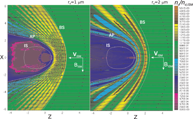
Figure 5: 2D distribution of the dust number density in the $({\bm{B}}_{\rm ISM},{\bm{V}}_{\rm ISM})$-plane for dust grains with $r_{\rm d}=1$ and $2\,\mu$m. The inner shock (IS), the astropause (AP) and the bow shock (BS) are shown by white lines. The streamlines (panel A) and the magnetic field lines (panel B) are plotted with black lines.

3.3 Synthetic maps of thermal dust emission

The astrosphere around $\kappa$ Cas, like the majority of other known astrospheres, is visible only via its infrared emission, whose origin can be attributed mostly to the thermal dust emission (e.g. van Buren & McCray 1988). To compare the model astrosphere with the Spitzer MIPS image we produce a synthetic map of thermal dust emission at $24\,\mu$m. For this, we integrate the local emissivity over the line of sight: $I_{\nu}(r_{\rm d})=\int j_{\rm\nu}(r_{{\rm d}},s)ds$, where $s$ is the coordinate along this line.

The local emissivity can be expressed as follows:

$$j_{\nu}(r_{\rm d},s)=\pi r_{\rm d}^{2}\,n_{\rm d}(s,r_{\rm d})Q_{\nu}(r_{\rm d})B_{\nu}(T_{\rm d}(s,r_{\rm d})),$$

where $n_{\rm d}$ is the dust number density, $Q_{\nu}$ is the dimensionless efficiency absorption factor of dust, $B_{\nu}$ is the Planck function, $T_{\rm d}$ is the dust temperature. $Q_{\nu}(r_{\rm d})$ is calculated using the Mie theory (Bohren & Huffman, 1983) for the chosen dust material. In this work, we consider astronomical silicates (Draine 2003), graphite (Draine 2003) and pure carbon (Jäger, Mutschke & Henning 1998). Plots of $Q_{\nu}(r_{d})$ for different materials and grain radii are presented in Fig. 6. The dust temperature can be calculated from local energy balance between dust heating by the stellar radiation and cooling due to thermal emission. Details of the temperature calculations are given in Appendix A. The obtained temperature depends on the grain material and radius, and the distance from the star (see Fig. 7).

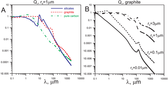
Figure 6: Dimensionless efficiency absorption factor of dust as a function of wavelength. A. $Q_{\nu}$ is presented for a fixed grain radius of 1 $\mu$m and different materials. B. $Q_{\nu}$ is presented for graphite grains with different radii.

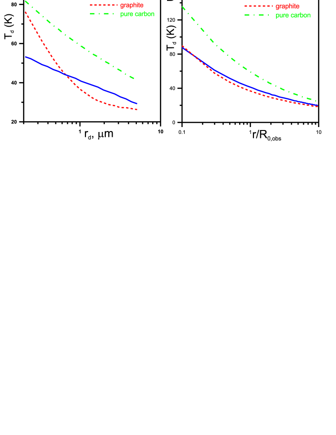
Figure 7: A. Dust temperature at a distance $r=1$ pc from the star as a function of the dust grain radius $r_{\rm d}$. B. Temperature of the dust grains with $r_{\rm d}=1\,\mu$m as a function of distance.

Dust number density can be represented as $n_{\rm d}(s,r_{\rm d})=\hat{n}_{d}(s,r_{\rm d})n_{\rm d,ISM}(r_{\rm d})$, where $\hat{n}_{\rm d}$ is the dimensionless dust number density taken from the model results. In the case of the MRN size distribution, the ISM number density of dust grains with radii in the range $[r_{\rm d}-{\rm d}r_{\rm d}/2;r_{\rm d}+{\rm d}r_{\rm d}/2]$ is ${\rm d}n_{\rm d,ISM}(r_{\rm d})=N_{\rm ISM}r_{\rm d}^{-3.5}dr_{\rm d}$. The dimensional coefficient $N_{\rm ISM}$ can be found from the assumption that the typical gas to dust mass ratio is equal to 100 (see Appendix B). Thus, the local emissivity of the dust grains with radii in the above range is

$${\rm d}j_{\nu}(s,r_{\rm d})=\pi r_{\rm d}^{2}\,Q_{\nu}(r_{\rm d})\,B_{\nu}(T_{\rm d}(s,r_{\rm d}))\,\hat{n}_{\rm d}(s,r_{\rm d})N_{\rm ISM}r_{\rm d}^{-3.5}\,{\rm d}r_{\rm d}$$

and the total intensity is:

$$I_{\nu}=\pi\,N_{\rm ISM}\,\int_{r_{\rm d,min}}^{r_{\rm d,max}}{\rm d}r_{\rm d}\int r_{\rm d}^{-1.5}\,Q_{\nu}(r_{\rm d})\,B_{\nu}(T_{\rm d}(s,r_{\rm d}))$$

$$\times\hat{n}_{\rm d}(s,r_{\rm d})\,ds.$$

We also performed calculations for certain dust grain radii with a uniform dust distribution in a narrow range $[r_{{\rm d},0}-dr_{\rm d}/2,r_{{\rm d},0}+dr_{\rm d}/2]$. In this case, in the formula for the total intensity $r_{\rm d}^{-1.5}$ should be replaced with $r_{{\rm d},0}^{2}$.

4 Comparison of the model results with observations and evaluation of the ISM parameters

To compare the model results with the observational data the intensity of the thermal dust emission should be calculated in the plane perpendicular to the line of sight. The orientation of the stellar velocity with respect to the line of sight is determined by two spherical angles $\theta$ and $\phi$ (see Fig. 8 for illustration). In our calculations the angle $\theta$ is fixed at 48$\degr$ (see Section 2), while the angle $\phi$ is a free parameter of the model because it is determined by the unknown orientation of the $({\bm{B}}_{\rm ISM},{\bm{V}}_{\rm ISM})$-plane. Therefore, we performed calculations at different planes and found that $\phi\approx 110-150\degr$ provides the best agreement with the observations. The results are presented for intermediate $\phi\approx 135\degr$.

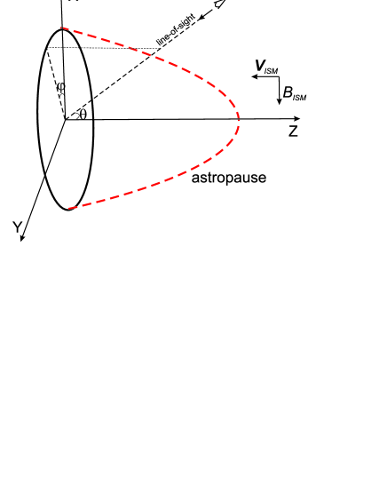
Figure 8: Schematic representation of observation of an astrosphere from an arbitrary line of sight. The astropause is shown by a red dashed line. The line of sight is characterized by two spherical angles: $\theta$ and $\phi$.

Fig. 9 plots the dust number density obtained for the MRN size distribution in the ISM with the range of grain sizes of $r_{\rm d}=0.2-3\,\mu$m. It is seen that no filaments are visible. The reason for this is that the filaments formed by dust grain with continuous size distribution merge with each other in a wide arcuate structure between the BS and the AP.

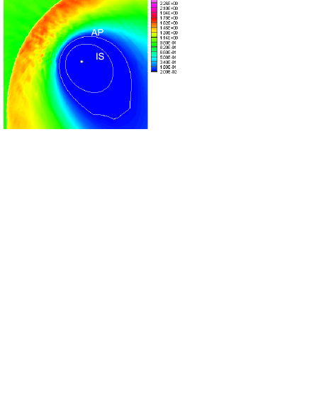
Figure 9: Dust number density in the observational plane for grains with the MRN size distribution in the range of $0.2-3\,\mu$m.

Before considering the intensity maps, we note that all our model calculations were performed in dimensionless form. In order to transform the dimensionless solution in the dimensional form and find absolute values of intensities one needs to specify the required dimensional parameters of the model (e.g. the characteristic distances and the dust number density in the ISM). This can be done in the following way. We assume that the brightest arc in the astrosphere around $\kappa$ Cas coincides with the astropause (our numerical calculations below support this assumption). By comparison of the obtained dimensionless solution with the known distance to the brightest arc, $R_{0}^{\rm obs}$, it is possible to determine the characteristic distance $D^{*}$, the corresponding ISM number density and the magnetic field strength, which are consistent with the observations and the model results. Namely, from the numerical modelling we know the dimensionless distance from the star to the astropause in the nose part of the astrosphere, $\hat{R_{0}}$, and:

$$R_{0}^{\rm obs}=\hat{R_{0}}D^{*}.$$

Combining this equation with equation (1) one has:

$$n_{\rm p,ISM}=\frac{\dot{M}v_{\infty}}{5.6\pi m_{\rm p}V_{\rm rel}^{2}}\left(\frac{\hat{R_{0}}}{R_{0}^{\rm obs}}\right)^{2}.$$

Then we obtain $B_{\rm ISM}$ from the Alfvenic Mach number:

$$B_{\rm ISM}=\frac{(5.6\pi m_{\rm p}n_{p,\rm ISM})^{1/2}V_{\rm rel}}{M_{\rm A,ISM}}.$$

The following estimates are obtained: $n_{\rm p,ISM}=3-11$ cm^-3, $B_{\rm ISM}=18-35\,\mu$ G. The ranges of $n_{\rm p,ISM}$ and $B_{\rm ISM}$ are due to uncertainties in $\dot{M}$ and $v_{\infty}$ of $\kappa$ Cas (see Table 1). From the gas to dust mass ratio of 100, one obtains the dust number density and the constant $N_{\rm ISM}$ (see Appendix B). Note that the intensity of the thermal dust emission is proportional to $N_{ISM}$, which in turn is proportional to $n_{\rm p,ISM}$. All intensity maps presented below are computed for the intermediate value of $n_{\rm p,ISM}=5$ cm^-3 and the corresponding uncertainties in intensity are a factor of few.

Fig. 10 shows the MIPS 24 $\mu$m image of the astrosphere around $\kappa$ Cas along with synthetic maps of emission from silicate, graphite and pure carbon dust grains at the same wavelength. All intensities are given in units of MJy sr^-1. Note that we added a constant intensity of 20 MJy sr^-1 to all synthetic maps to mimic the background emission that is seen in the data. It is seen that for all types of dust grains there is a maximum of intensity at the nose part of the astrosphere close to the astropause. However, no separate filaments are visible. This is explained by two effects. The first one is the same as was discussed above for the distribution of the dust number density – no filaments can be distinguished for the mixture of dust grains with the MNR size distribution. For the intensity maps this effect is even more pronounced than for the number density. The reason is that small dust grains are more heated than the larger ones and therefore their contribution to the total emission intensity is larger. In our model the filaments are clearly seen for grains with radii $r_{\rm d}=1-2\,\mu$m. But these large grains are too cool to contribute to the total intensity maps. Note that the temperature of carbon grains is much higher than the temperature of silicon and graphite ones (Fig. 7), but this is still not enough to make filaments visible because the efficiency absorption factor $Q_{\nu}$ at 24 $\mu$m for carbon is much smaller than that for graphite and silicon (see Fig. 6).

The second effect is connected with the distribution of the dust temperature, which decreases with distance from the star because the dust grains are heated mostly by the stellar radiation. Correspondingly, the intensity of the thermal dust emission, which is proportional to the Planck function, is a strong function of temperature and hence of the distance from the star. As a result, the thermal dust emission near the AP is much stronger than near the BS.

Fig. 10 also shows that the emission intensity ratio of the brightest arc of the astrosphere to the background is about an order of magnitude smaller compared with the observations.

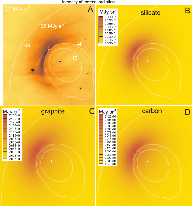
Figure 10: A. MIPS 24 $\mu$m image of the astrosphere around $\kappa$ Cas with white lines indication the position of discontinuities (IS, AP and BS) in the model astrosphere. B–D. Synthetic intensity maps of the thermal dust emission at $24\,\mu$m for silicates, graphite and pure carbon. The model results are obtained for dust with the MRN size distribution with the range of grain sizes of $0.2-3\,\mu$m and the dust temperature calculated from the local energy balance equation.

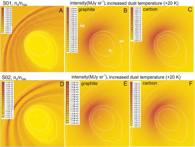
Figure 11: Model results obtained for two narrow ranges of grain radii (SO1: $r_{d}\in[1.3,1.7]\,\mu$m and SO2: $r_{d}\in[1.8,2.2]\,\mu$m). Plots A and D present dust number density in dimensionless units. Plots B, C, E and F present intensity maps for graphite and carbon. The results are obtained with the dust temperature increased by 20 K everywhere. Discontinuities are shown by white lines.

Thus, we found that the observed filamentary structure cannot be explained in the framework of the model with the classical MRN size distribution. The actual dust size distribution however could differ from the MRN one. For example, Wang, Li & Jiang (2015) reported that the existence of the very large ($0.5-6\,\mu$m) dust grains in the ISM is confirmed by several independent observational evidences (see also Lehtinen & Mattila 1996; Pagani et al. 2010; Steinacker et al. 2015). Moreover, Wang et al. (2015) noted that “if a substantial fraction of interstellar dust is from supernova condensates, then $\mu$m-sized grains may be prevalent in the ISM”.

Assuming that the large dust grains are indeed prevail in the local ISM, we examine the range of dust parameters for which one can reproduce the observed filamentary structure of the astrosphere around $\kappa$ Cas. In particular, we assumed that the dust in the local ISM is composed only of big grains (with the gas to dust mass ratio of 100) and performed calculations for two narrow ranges of grain sizes with uniform distribution inside each range: $r_{\rm d}\in[1.3,1.7]\,\mu$m and $r_{\rm d}\in[1.8,2.2]\,\mu$m; hereafter ranges SO1 and SO2, respectively. Figs 11 A and 11 D plot the distributions of the dust number density in the observational plane for graphite and carbon grains with radii in the above two ranges. One can discern five and three filaments, respectively, for SO1 and SO2. The filaments are wider than in Fig. 5 because now we consider a range of grain radii, while Fig. 5 was obtained for grains of a particular radius. We also calculated corresponding intensity maps, but the filaments do not appear on them because of the low dust temperature, which rapidly decreases with distance from the star (we do not show these maps since they are very similar to those shown in Fig. 10). The temperature obtained as a solution of the local energy balance (see Appendix A) is high enough to produce filaments in the intensity maps at 24 $\mu$m only in a narrow region close to the astropause, while at larger distances the dust emission at this wavelength is rapidly deceases.

We speculate that the dust grains might be hotter due to some additional heating processes. To check how this will affect the intensity maps, we artificially increased the dust temperature for both graphite and carbon grains by 20 K everywhere in the astrosphere. The resulting emission maps are presented in Figs 11 B–C and 11 E–F for both ranges of grain sizes SO1 and SO2. One can see that with the increase of the dust temperature the filaments become more pronounced. Qualitatively, these intensity maps are quite similar to the MIPS image of the astrosphere around $\kappa$ Cas. The absolute values of the emission intensity are also similar to the observed ones (recall that the calculated intensity is accurate within a factor of few due to the uncertainty in the ISM plasma density estimate). We note also that the dust density maximum visible near the BS in the panels A and D of Fig. 11 is absent in the intensity maps. This is again because of small dust temperature in this remote part of the astrosphere.

Finally, we note that the smaller the dust grains the higher their temperature (see the panel A in Fig. 7), which implies that one can avoid the artificial increase of the dust temperature if one adopts smaller dust grain radii. On the other hand, to make the filaments observable, one needs to keep the same separation between them, which for the given dust grain radius is inversely proportional to the magnetic field strength and the dust surface potential (see equation (3)). From this it follows that the decrease of the grain size should be compensated by decrease of $B$ or $U_{\rm d,ISM}$ (or both). A strong decrease of the magnetic field strength, however, is less appropriate because, as discussed above, this would lead to the collapse of the outer shock region. The surface potential of the dust grains is, in principle, a free parameter of the model and many different processes can affect its value. If one adopts a factor of 10 smaller potential, then to produce the same number of filaments the radii of the dust grains could be a factor of $\approx 3$ smaller than those adopted in our modelling. Such grains are hot enough to produce observable filaments in the intensity maps.

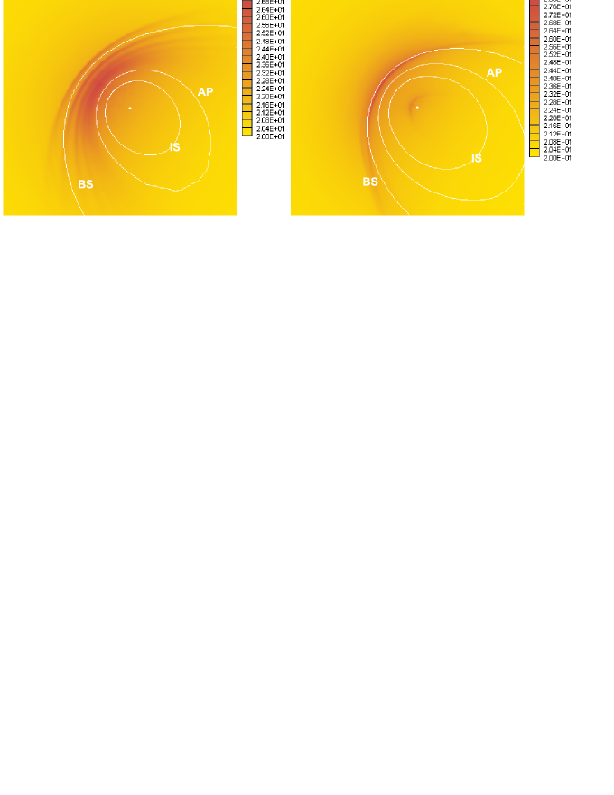
Figure 12: Maps of the thermal dust emission calculated for graphite dust grains with radii in the range $r_{\rm d}=1.45-1.55\,\mu$m and temperatures artificially increased by 20 K. Plots in panels A and B correspond to models with $M_{\rm A,ISM}$=3 and 12, respectively. $M_{\rm ISM}=3$ in both models.

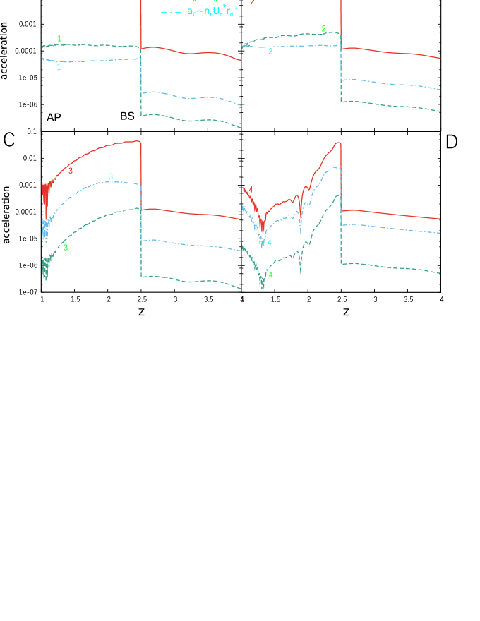
Figure 13: Dimensionless acceleration ($F/m_{\rm d}$ normalized to $180V_{\rm ISM}^{2}/R_{\rm obs}$) of a dust grain (with radius of 1 $\mu$m) along its trajectory caused by the Lorentz force (red curves), the direct drag force (green curves) and the Coulomb drag force (blue curves). The results presented in panels A–D were obtained, respectively, for the following four pairs of values of the proton number density and initial dust surface potential: 1) $n_{\rm p,ISM}=3\,{\rm cm}^{-3},U_{\rm d,ISM}$=0.75 V; 2) $n_{\rm p,ISM}=10\,{\rm cm}^{-3},U_{\rm d,ISM}$=0.75 V; 3) $n_{\rm p,ISM}=3\,{\rm cm}^{-3},U_{\rm d,ISM}=-1.3$ V, and 4) $n_{\rm p,ISM}=10\,{\rm cm}^{-3},U_{\rm d,ISM}=-$1.6 V.

5 Summary and discussion

In this paper, we performed 3D MHD numerical modelling of the astrosphere around $\kappa$ Cas in order to produce a synthetic map of its thermal dust emission at 24 $\mu$m and to explain its filamentary structure. We found that distinct filaments would appear in the emission map only if quite large ($\mu$m-sized) dust grains are prevalent in the local ISM. The filamentary structure is not seen for continuous power-law size distribution of dust because individual filaments merge with each other due to the influence of small grains. Our model with large (1.3-2.2 $\mu$m) graphite and pure carbon dust grains reproduces the observational data quite well, if the temperature of these grains in the region where the filaments are formed is about 40 and 75 K, respectively. Comparison of the observed distance from the star to the brightest arc in the astrosphere with the model results allows us to estimate the ISM number density to be $3-11\,{\rm cm}^{-3}$. We also constrain the local interstellar magnetic field strength to be $18-35\,\mu$G, which exceeds the typical field strength in the warm phase of the ISM (Troland & Heiles 1986; Harvey-Smith et al. 2011).

We performed test calculations with larger Alfvenic Mach numbers $M_{\rm A,ISM}$=3 and 12 that corresponds to weaker interstellar magnetic field (10 and 2.7 $\mu$G, respectively, for $n_{\rm p,ISM}$=3 cm^-3). The synthetic maps of thermal dust emission for graphite dust grains with radii of $1.45-1.55\,\mu$m are presented in Fig. 12. In this figure the filaments are more distinct compared to, e.g., Fig. 11 because the more narrow range of grain radii is considered. For smaller $B_{\rm ISM}$ the outer shock layer (confined between the BS and the AP) becomes thinner. The model with $M_{\rm A,ISM}$=3 is still appropriate: the filaments are seen and the emission intensity is close to the observed one. Note that the outermost filament in the panel A of Fig. 12 is in fact located between the AP and the BS, and appears beyond the BS because of the projection effect. The model with $M_{\rm A,ISM}$=12 provides a too small separation between the AP and the BS, so that the filaments merge with each other and the model cannot reproduce the observations for any grain size distribution. It is also interesting to note that there is a small arc close to the star in the case of weak magnetic field ($M_{\rm A,ISM}$=12). This arc is formed by large dust grains penetrating inside the IS. Near the star these grains are swept out by the stellar radiation and appear as an arc.

Our numerical calculations are performed under assumption of constant dust charge. In general, the grain charge is determined by the balance between three main processes: impinging of protons and electrons, secondary electron emission due to electron impacts (this is especially important for hot plasma with $T\ga 10^{5}$ K) and photoelectron emission caused by the external interstellar and stellar radiation. We performed estimations of the changes of the dust charge and found that they are not more than 30 per cent in the considered region between the BS and the AP. Therefore we can neglect them and assume that the dust grain charge does not vary along the trajectory.

In our calculations, we neglected the drag forces caused by direct collisions of the dust grains with ions and electrons (direct drag force), and by the electromagnetic Coulomb interaction (Coulomb drag force), although our numerical model allows us to take them into account. Ochsendorf et al. (2014) found that the Coulomb drag force can affect the formation of so-called “dust waves” – arclike enhancements of dust density around weak-wind stars – created because of decoupling of the dust grains from the gas by stellar radiation force. Namely, they showed that inclusion of the Coulomb drag in the model leads to a strong dust-gas coupling, which prevents the formation of the dust waves. To clarify whether or not the drag forces could be important in our calculations, below we discuss the model parameters which determine their relative contributions to the dust motion in the astrosphere. Fig. 13 shows accelerations ($a=F/m_{\rm d}$) of a dust grain (with radius $r_{\rm d}=1\,\mu$m) along its trajectory due to three forces: the Lorentz force ($a_{\rm L}$), the direct drag force ($a_{\rm R}$) and the Coulomb drag force ($a_{\rm C}$). Note that $a_{\rm L}\sim q/m_{\rm d}\sim U_{\rm d}/r_{\rm d}^{2}$, $a_{\rm R}\sim n_{\rm p}/r_{\rm d}$, and $a_{\rm C}\sim n_{\rm p}U_{\rm d}^{2}/r_{\rm d}$. These relations determine the balance between different forces for the chosen model parameters. Accelerations are calculated for the following four pairs of values of the proton number density and the initial dust surface potential: $n_{\rm p,ISM}=3\,{\rm cm}^{-3},U_{\rm d,ISM}=0.75$ V (hereafter, case 1; see panel A in Fig. 13), $n_{\rm p,ISM}=10\,{\rm cm}^{-3},U_{\rm d,ISM}$=0.75 V (case 2; panel B), $n_{\rm p,ISM}=3\,{\rm cm}^{-3},U_{\rm d,ISM}=-1.3$ V (case 3; panel C), and $n_{\rm p,ISM}=10\,{\rm cm}^{-3},U_{\rm d,ISM}=-1.6$ V (case 4; panel D). It is seen from Fig. 13 that in cases 3 and 4 the Coulomb drag force is larger than the direct drag force because of the large potential of the dust grains. One can see also that the Lorentz force is by one-two orders of magnitude larger than the drag forces in cases 1–3 and becomes comparable to the Coulomb drag force in case 4. Thus, it is seen that for the parameters considered in our paper ($n_{\rm p,ISM}=3-11\,{\rm cm}^{-3}$ and $U_{\rm d,ISM}$=0.75 V) the influence of the drag forces can be safely neglected. However, for higher gas densities and/or dust potentials their effect could be significant.

Our explanation of the cirrus-like structure of the astrosphere around $\kappa$ Cas implies that the thermal mid-IR emission of the dust originates in regions spatially separated from the region of the bulk optical line emission. Also, we expect that in the optical wavelengths the astrosphere should have a smooth appearance, unless it is deformed by (magneto)hydrodynamic instabilities. But even in this case, the optical filaments should not correlate with the mid-IR cirrus-like ones. In principle, the difference between the mid-IR and optical appearances of an astrosphere could be detected, provided that it is nearby enough to allow us to resolve the layer between the astropause and the bow shock. Unfortunately, with the existing optical surveys we were not able to detect the optical counterpart of the astrosphere of $\kappa$ Cas, particularly because this bright ($V\approx 4$ mag) star outshines all around it. Optical imaging with narrow-band filters could potentially be of value in detection of the astrosphere and in verifying our model.

We realize that the mechanism for origin of the filamentary structure of astrospheres is not unique and that the observed filaments might be produced by various different processes. For example, they could arise because of the rippling effect in radiative shocks, i.e. due to variations in the projection of the shock velocity along the line of sight (Hester 1987). Also, the filaments could originate because of time-dependent variations of the wind velocity (Decin et al. 2006) or might be caused by instabilities in the bow shock and contact discontinuity (Dgani, Van Buren & Noriega-Crespo 1996). Numerical simulations by many authors (e.g., van Marle et al. 2011, 2014; Mackey et al. 2012; Meyer et al. 2014a,b; Acreman et al. 2016) indeed show that astrospheres may be subject to various types of instabilities. However, it is a challenge to separate the real instabilities from the numerical ones, and we refrain in this paper from discussing this problem in depth.

To conclude, we note that our model does not explain the origin of the almost straight filaments in the south part of the astrosphere, which intersect the brightest arc at almost right angle (see Fig. 1). These filaments might be due to much more complex structure of the interstellar magnetic field than assumed in our modelling (cf. Gvaramadze et al. 2011b). Also, inspection of the WISE 22 $\mu$m image of the region around $\kappa$ Cas shows that these filaments have the same orientation as an elongated pillar to the west of the star (see Fig. 14), which points to the possibility that their origin might be due to interaction of the astrosphere with the inhomogeneous local ISM. Modelling of this interaction is, however, beyond the scope of the present paper.

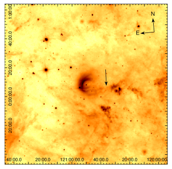
Figure 14: $1\degr\times 1\degr$ WISE 22 $\mu$m image of the field containing $\kappa$ Cas and its astrosphere. The pillar to the west of $\kappa$ Cas is indicated by an arrow (see text for details). The coordinates are the Galactic longitude and latitude on the horizontal and vertical scales, respectively. At a distance of 1 kpc, $1\degr$ corresponds to $\approx 17$ pc.

Appendix A Calculation of dust temperature

The dust temperature in the astrosphere can be found by solving the dust thermal balance for equilibrium. This approach is justified because the heating and cooling time-scales are shorter than the characteristic time-scale of dust grain motion in the astrosphere. We do not consider the radiative transfer and multiple scattering of photons because of small dust number density that allows us to use an optically thin approximation. The dust grains are heated due to absorption of stellar and interstellar radiation, while their cooling is caused mostly by thermal black body emission. The energy balance for a single dust grain can be stated as follows (see, e.g., Hocuk et al. 2017):

$$4\pi\,r_{\rm d}^{2}\,\int_{0}^{\infty}Q_{\nu}B_{\nu}(T_{\rm d})\,d\nu=r_{\rm d}^{2}\,\int_{0}^{\infty}Q_{\nu}F^{*}_{\nu}(r,T_{*})\,d\nu+$$ (4)

$$+2\pi\,r_{\rm d}^{2}\,\int_{0}^{\infty}Q_{\nu}J_{\nu}\,d\nu,$$

where $F^{*}_{\nu}=\pi\,(R_{*}/r)^{2}B_{\nu}(T_{*})$ is the stellar radiation at point $r$, $J_{\nu}$ is the intensity of the isotropic stellar radiation field (see fig. 2 in Hocuk et al. 2017). $R_{*}$ and $T_{*}$ for $\kappa$ Cas are given in Table 1. Equation (A) is solved numerically and $T_{\rm d}$ is found for any grain radii $r_{\rm d}$ and distances $r$.

Appendix B Dust number density in the ISM

In the case of power-law size distribution, the ISM number density of dust grains with radius of $[r_{d}-dr_{d}/2;r_{d}+dr_{d}/2]$ is $dn_{\rm ISM}(r_{\rm d})=N_{\rm ISM}r_{\rm d}^{-3.5}dr_{\rm d}$ and their mass density is $d\rho_{\rm d,ISM}=m_{\rm d}\,dn_{\rm d,ISM}(r_{\rm d})$. $m_{\rm d}=4/3\pi\,r_{\rm d}^{3}\,\rho_{\rm d}$ is the mass of a dust grain, $\rho_{\rm d}=2.5\,{\rm g}\,{\rm cm}^{-3}$ is a typical mass density for the interstellar grain material. We assume that the gas to dust mass ratio in the ISM is about 100. The mass density of the dust in the ISM is:

$$\rho_{\rm d,ISM}=\frac{4}{3}\pi\rho_{\rm d}N_{\rm ISM}\int_{r_{\rm d,min}}^{r_{\rm d,max}}r_{\rm d}^{-0.5}dr_{\rm d}.$$

For the gas to dust mass ratio of $\rho_{\rm p,ISM}/\rho_{\rm d,ISM}=100$, one has

$$N_{\rm ISM}=\frac{3}{800\pi}\frac{\rho_{\rm p,ISM}}{\rho_{\rm d}}\frac{1}{r_{\rm d,max}^{0.5}-r_{\rm d,min}^{0.5}}.$$

Note that $[N_{\rm ISM}]={\rm cm}^{-0.5}$.

References

- [1] Acreman D. M., Stevens I. R., Harries T. J., 2016, MNRAS, 456, 136
- [2] Akimkin V. V., Kirsanova M. S., Pavlyuchenkov Ya. N., Wiebe D. S., 2015, MNRAS, 449, 440
- [3] Alexashov D. B., Katushkina O. A., Izmodenov V. V., Akaev P. S., 2016, MNRAS, 458, 2553
- [4] Blaauw A., 1961, Bull. Astron. Inst. Netherlands, 15, 265
- [5] Bohren C. F., Huffman D. R., 1983, Absorption and scattering of light by small particles, ISBN: 978-0-471-29340-8
- [6] Cowie L. L., McKee C. F., Ostriker J. P., 1981, Astrophys. J., 247, 908
- [7] Cox N. L. G. et al., 2012, A&A, 537, A35
- [8] Crowther P. A., Lennon D. J., Walborn N. R., 2006, A&A, 446, 279
- [9] Decin L., Hony S., de Koter A., Tielens A. G. G. M., Waters L. B. F. M., 2006, A&A, 456, 549
- [10] Dgani R., Van Buren D., Noriega-Crespo A., 1996, ApJ, 461, 372
- [11] Draine B. T., 2003, ApJ, 598, 1026
- [12] Draine B. T., Salpeter E. E., 1979, ApJ, 231, 77
- [13] Gontcharov G. A., 2006, Astron. Lett., 32, 759
- [14] Grün E., Svestka J., 1996, SSRev, 78, 347
- [15] Gvaramadze V. V., Bomans D. J., 2008, A&A, 490, 1071
- [16] Gvaramadze V. V., Pflamm-Altenburg J., Kroupa P., 2011, A&A, 525, A17
- [17] Gvaramadze V. V., Röser S.; Scholz R.-D., Schilbach E., 2011a, A&A, 529, A14
- [18] Gvaramadze V. V., Kniazev A. Y., Kroupa P., Oh S., 2011b, A&A, 535, A29
- [19] Gvaramadze V. V., Mackey J., Kniazev A. Y., Langer N., Chené A.-N., Castro N., Haworth T. J., Grebel E. K., 2017, MNRAS, 466, 1857
- [20] Harvey-Smith L., Madsen G. J., Gaensler B. M., 2011, ApJ, 736, 83
- [21] Hester J. J., 1987, ApJ, 314, 187
- [22] Hocuk S., Szucs L., Caselli P., Cazaux S., Spaans M., Esplugues G. B., 2017, preprint (arXiv:1704.02763)
- [23] Humphreys R. M., 1978, ApJS, 38, 309
- [24] Jäger C., Mutschke H., Henning Th., 1998, A&A, 332, 291
- [25] Katushkina O. A., Alexashov D. B., Izmodemov V. V., Gvaramadze V. V., 2017, MNRAS, 465, 1573 (Paper I)
- [26] Kimura H., Mann I., 1998, ApJ, 499, 454
- [27] Kobulnicky H. A. et al., 2016, ApJS, 227, 18
- [28] Lehtinen K., Mattila K., 1996, A&A, 309, 570
- [29] Mackey J., Gvaramadze V. V., Mohamed S., Langer N., 2015, A&A, 573, A10
- [30] Mackey J., Mohamed S., Neilson H. R., Langer N., Meyer D. M.-A., 2012, ApJ, 751, L10
- [31] Mackey J., Haworth T. J., Gvaramadze V. V., Mohamed S., Langer N., Harries T. J., 2016, A&A, 586, A114
- [32] Mathis J. S., Rumpl W., Nordsieck K. H., 1977, ApJ, 217, 425
- [33] Megier A., Strobel A., Galazutdinov G. A., Krelowski J., 2009, A&A, 507, 833
- [34] Meyer D. M.-A., Gvaramadze V. V., Langer N., Mackey J., Boumis P., Mohamed S., 2014a, MNRAS, 439, L41
- [35] Meyer D. M.-A., Mackey J., Langer N., Gvaramadze V. V., Mignone A., Izzard R. G., Kaper L., 2014b, MNRAS, 444, 2754
- [36] Mel’nik A. M., Dambis A. K., 2009, MNRAS, 400, 518
- [37] Ochsendorf B. B., Cox N. L. J., Krijt S., Salgado F., Berné O., Bernard J. P., Kaper L., Tielens A. G. G. M., 2014, A&A, 563, A65
- [38] Pagani L., Steinacker J., Bacmann A., Stutz A., Henning T., 2010, Science, 329, 1622
- [39] Pandey A. K., Sharma S., Ogura K., Ojha D. K., Chen W. P., Bhatt B. C., Ghosh S. K., 2008, MNRAS, 383, 1241
- [40] Pavlyuchenkov Y. N., Kirsanova M. S., Wiebe D. S., 2013, Astron. Rep., 57, 573
- [41] Peri C. S., Benaglia P., Brookes D. P., Stevens I. R., Isequilla N. L., 2012, A&A, 538, 108
- [42] Reid M. J., Menten K. M., Zheng X. W., Brunthaler A., Xu Y., 2009, ApJ, 705, 1548
- [43] Rieke G. H. et al., 2004, ApJS, 154, 25
- [44] Searle S. C., Prinja R. K., Massa D., Ryans R., 2008, A&A, 481, 777
- [45] Schönrich R., Binney J., Dehnen W., 2010, MNRAS, 403, 1829
- [46] Steinacker J. et al., 2015, A&A, 582, A70
- [47] Troland T. H., Heiles C., 1986, ApJ, 301, 339
- [48] van Buren D., McCray R., 1988, ApJ, 329, L93
- [49] van Buren D., Noriega-Crespo A., Dgani R., 1995, AJ, 110, 2914
- [50] van Leeuwen F., 2007, A&A, 474, 653
- [51] van Marle A. J., Meliani Z., Keppens R., Decin L., 2011, ApJ, 734, L26
- [52] van Marle A. J., Decin L., Meliani Z., 2014, A&A, 561, A152
- [53] Walborn N. R., 1972, AJ, 77, 312
- [54] Wang S., Li A., Jiang B. W., 2015, ApJ, 811, 38
- [55] Wolf B., 1989, A&A, 217, 87