Measurement of the tau Michel parameters and
in the radiative leptonic decay
Belle preprint 2017-20, KEK preprint 2017-29
\nameN. Shimizu75
\nameH. Aihara75
\nameD. Epifanov3,59
\nameI. Adachi15,11
\nameS. Al Said69,34
\nameD. M. Asner61
\nameV. Aulchenko3,59
\nameT. Aushev49
\nameR. Ayad69
\nameV. Babu70
\nameI. Badhrees69,33
\nameA. M. Bakich68
\nameV. Bansal61
\nameE. Barberio47
\nameV. Bhardwaj17
\nameB. Bhuyan19
\nameJ. Biswal29
\nameA. Bobrov3,59
\nameA. Bozek56
\nameM. Bračko45,29
\nameT. E. Browder14
\nameD. Červenkov4
\nameM.-C. Chang9
\nameP. Chang55
\nameV. Chekelian46
\nameA. Chen53
\nameB. G. Cheon13
\nameK. Chilikin40,48
\nameK. Cho35
\nameS.-K. Choi12
\nameY. Choi67
\nameD. Cinabro80
\nameT. Czank73
\nameN. Dash18
\nameS. Di Carlo80
\nameZ. Doležal4
\nameD. Dutta70
\nameS. Eidelman3,59
\nameJ. E. Fast61
\nameT. Ferber7
\nameB. G. Fulsom61
\nameR. Garg62
\nameV. Gaur79
\nameN. Gabyshev3,59
\nameA. Garmash3,59
\nameM. Gelb31
\nameP. Goldenzweig31
\nameD. Greenwald71
\nameE. Guido27
\nameJ. Haba15,11
\nameK. Hayasaka58
\nameH. Hayashii52
\nameM. T. Hedges14
\nameS. Hirose50
\nameW.-S. Hou55
\nameT. Iijima51,50
\nameK. Inami50
\nameG. Inguglia7
\nameA. Ishikawa73
\nameR. Itoh15,11
\nameM. Iwasaki60
\nameI. Jaegle8
\nameH. B. Jeon38
\nameS. Jia2
\nameY. Jin75
\nameK. K. Joo5
\nameT. Julius47
\nameK. H. Kang38
\nameG. Karyan7
\nameT. Kawasaki58
\nameC. Kiesling46
\nameD. Y. Kim65
\nameJ. B. Kim36
\nameS. H. Kim13
\nameY. J. Kim35
\nameK. Kinoshita6
\nameP. Kodyš4
\nameS. Korpar45,29
\nameD. Kotchetkov14
\nameP. Križan41,29
\nameR. Kroeger25
\nameP. Krokovny3,59
\nameR. Kulasiri32
\nameA. Kuzmin3,59
\nameY.-J. Kwon82
\nameJ. S. Lange10
\nameI. S. Lee13
\nameL. K. Li22
\nameY. Li79
\nameL. Li Gioi46
\nameJ. Libby20
\nameD. Liventsev79,15
\nameM. Masuda74
\nameM. Merola26
\nameK. Miyabayashi52
\nameH. Miyata58
\nameG. B. Mohanty70
\nameH. K. Moon36
\nameT. Mori50
\nameR. Mussa27
\nameE. Nakano60
\nameM. Nakao15,11
\nameT. Nanut29
\nameK. J. Nath19
\nameZ. Natkaniec56
\nameM. Nayak80,15
\nameM. Niiyama37
\nameN. K. Nisar63
\nameS. Nishida15,11
\nameS. Ogawa72
\nameS. Okuno30
\nameH. Ono57,58
\nameG. Pakhlova40,49
\nameB. Pal6
\nameC. W. Park67
\nameH. Park38
\nameS. Paul71
\nameT. K. Pedlar43
\nameR. Pestotnik29
\nameL. E. Piilonen79
\nameV. Popov49
\nameM. Ritter42
\nameA. Rostomyan7
\nameY. Sakai15,11
\nameM. Salehi44,42
\nameS. Sandilya6
\nameY. Sato50
\nameV. Savinov63
\nameO. Schneider39
\nameG. Schnell1,16
\nameC. Schwanda23
\nameY. Seino58
\nameK. Senyo81
\nameM. E. Sevior47
\nameV. Shebalin3,59
\nameT.-A. Shibata76
\nameJ.-G. Shiu55
\nameB. Shwartz3,59
\nameA. Sokolov24
\nameE. Solovieva40,49
\nameM. Starič29
\nameJ. F. Strube61
\nameK. Sumisawa15,11
\nameT. Sumiyoshi77
\nameU. Tamponi27,78
\nameK. Tanida28
\nameF. Tenchini47
\nameK. Trabelsi15,11
\nameM. Uchida76
\nameT. Uglov40,49
\nameY. Unno13
\nameS. Uno15,11
\nameY. Usov3,59
\nameC. Van Hulse1
\nameG. Varner14
\nameV. Vorobyev3,59
\nameA. Vossen21
\nameC. H. Wang54
\nameM.-Z. Wang55
\nameP. Wang22
\nameM. Watanabe58
\nameE. Widmann66
\nameE. Won36
\nameY. Yamashita57
\nameH. Ye7
\nameC. Z. Yuan22
\nameZ. P. Zhang64
\nameV. Zhilich3,59
\nameV. Zhukova40,48
\nameV. Zhulanov3,59
\nameA. Zupanc41,29
1
2
3
4
5
6
7
8
9
10
11
12
13
14
15
16
17
18
19
20
21
22
23
24
25
26
27
28
29
30
31
32
33
34
35
36
37
38
39
40
41
42
43
44
45
46
47
48
49
50
51
52
53
54
55
56
57
58
59
60
61
62
63
64
65
66
67
68
69
70
71
72
73
74
75
76
77
78
79
80
81
82
University of the Basque Country UPV/EHU, 48080 Bilbao
Beihang University, Beijing 100191
Budker Institute of Nuclear Physics SB RAS, Novosibirsk 630090
Faculty of Mathematics and Physics, Charles University, 121 16 Prague
Chonnam National University, Kwangju 660-701
University of Cincinnati, Cincinnati, Ohio 45221
Deutsches Elektronen–Synchrotron, 22607 Hamburg
University of Florida, Gainesville, Florida 32611
Department of Physics, Fu Jen Catholic University, Taipei 24205
Justus-Liebig-Universität Gießen, 35392 Gießen
SOKENDAI (The Graduate University for Advanced Studies), Hayama 240-0193
Gyeongsang National University, Chinju 660-701
Hanyang University, Seoul 133-791
University of Hawaii, Honolulu, Hawaii 96822
High Energy Accelerator Research Organization (KEK), Tsukuba 305-0801
IKERBASQUE, Basque Foundation for Science, 48013 Bilbao
Indian Institute of Science Education and Research Mohali, SAS Nagar, 140306
Indian Institute of Technology Bhubaneswar, Satya Nagar 751007
Indian Institute of Technology Guwahati, Assam 781039
Indian Institute of Technology Madras, Chennai 600036
Indiana University, Bloomington, Indiana 47408
Institute of High Energy Physics, Chinese Academy of Sciences, Beijing 100049
Institute of High Energy Physics, Vienna 1050
Institute for High Energy Physics, Protvino 142281
University of Mississippi, University, Mississippi 38677
INFN - Sezione di Napoli, 80126 Napoli
INFN - Sezione di Torino, 10125 Torino
Advanced Science Research Center, Japan Atomic Energy Agency, Naka 319-1195
J. Stefan Institute, 1000 Ljubljana
Kanagawa University, Yokohama 221-8686
Institut für Experimentelle Kernphysik, Karlsruher Institut für Technologie, 76131 Karlsruhe
Kennesaw State University, Kennesaw, Georgia 30144
King Abdulaziz City for Science and Technology, Riyadh 11442
Department of Physics, Faculty of Science, King Abdulaziz University, Jeddah 21589
Korea Institute of Science and Technology Information, Daejeon 305-806
Korea University, Seoul 136-713
Kyoto University, Kyoto 606-8502
Kyungpook National University, Daegu 702-701
École Polytechnique Fédérale de Lausanne (EPFL), Lausanne 1015
P.N. Lebedev Physical Institute of the Russian Academy of Sciences, Moscow 119991
Faculty of Mathematics and Physics, University of Ljubljana, 1000 Ljubljana
Ludwig Maximilians University, 80539 Munich
Luther College, Decorah, Iowa 52101
University of Malaya, 50603 Kuala Lumpur
University of Maribor, 2000 Maribor
Max-Planck-Institut für Physik, 80805 München
School of Physics, University of Melbourne, Victoria 3010
Moscow Physical Engineering Institute, Moscow 115409
Moscow Institute of Physics and Technology, Moscow Region 141700
Graduate School of Science, Nagoya University, Nagoya 464-8602
Kobayashi-Maskawa Institute, Nagoya University, Nagoya 464-8602
Nara Women’s University, Nara 630-8506
National Central University, Chung-li 32054
National United University, Miao Li 36003
Department of Physics, National Taiwan University, Taipei 10617
H. Niewodniczanski Institute of Nuclear Physics, Krakow 31-342
Nippon Dental University, Niigata 951-8580
Niigata University, Niigata 950-2181
Novosibirsk State University, Novosibirsk 630090
Osaka City University, Osaka 558-8585
Pacific Northwest National Laboratory, Richland, Washington 99352
Panjab University, Chandigarh 160014
University of Pittsburgh, Pittsburgh, Pennsylvania 15260
University of Science and Technology of China, Hefei 230026
Soongsil University, Seoul 156-743
Stefan Meyer Institute for Subatomic Physics, Vienna 1090
Sungkyunkwan University, Suwon 440-746
School of Physics, University of Sydney, New South Wales 2006
Department of Physics, Faculty of Science, University of Tabuk, Tabuk 71451
Tata Institute of Fundamental Research, Mumbai 400005
Department of Physics, Technische Universität München, 85748 Garching
Toho University, Funabashi 274-8510
Department of Physics, Tohoku University, Sendai 980-8578
Earthquake Research Institute, University of Tokyo, Tokyo 113-0032
Department of Physics, University of Tokyo, Tokyo 113-0033
Tokyo Institute of Technology, Tokyo 152-8550
Tokyo Metropolitan University, Tokyo 192-0397
University of Torino, 10124 Torino
Virginia Polytechnic Institute and State University, Blacksburg, Virginia 24061
Wayne State University, Detroit, Michigan 48202
Yamagata University, Yamagata 990-8560
Yonsei University, Seoul 120-749
Abstract
We present a measurement of the Michel parameters of the lepton,
and , in the radiative leptonic
decay
using 711 f of collision data collected
with the Belle detector at the KEKB collider.
The Michel parameters are measured in an unbinned maximum likelihood fit
to the kinematic distribution
of
or . The measured values of the Michel parameters
are and ,
where the first error is statistical and the second
is systematic. This is the first measurement of these parameters.
These results are consistent
with the Standard Model predictions within their uncertainties and
constrain the coupling constants of the generalized weak interaction.
\subjectindex
C01, C07, C21
1 Introduction
In the Standard Model (SM), there are three flavors of charged leptons:
, and . The SM has proven to be the fundamental theory in
describing the physics of particles;
nevertheless, precision tests may reveal the presence of physics
beyond the Standard Model (BSM).
In particular, a measurement of Michel parameters in leptonic and radiative leptonic
decays is a powerful probe for the BSM contributions [1, 2].
The most general Lorentz-invariant derivative-free matrix element
of leptonic decay
***Unless otherwise stated, use of charge-conjugate modes is implied
throughout the paper. is represented as [3]
where is the Fermi constant, and are the chirality
indices for the charged leptons, and are the chirality indices
of the neutrinos, is or , ,
, and
are, respectively, the scalar, vector and tensor Lorentz structures
in terms of the Dirac matrices , and are the
four-component spinors of a particle and an antiparticle, respectively,
and are the corresponding dimensionless couplings.
In the SM, decays into and a -boson,
the latter decays into and right-handed ;
i.e., the only non-zero coupling is .
Experimentally, only the squared matrix element is observable and
bilinear combinations of the are accessible.
Of all such combinations, four Michel parameters, , ,
, and , can be measured in the leptonic decay of the
when the final-state neutrinos are not observed and the spin of the outgoing lepton is not measured [4]:
Figure 1: Three Feynman diagrams of the tau radiative leptonic decay
The Feynman diagrams describing the radiative leptonic decay of the
are presented in Fig. 1.
The last amplitude is ignored because this contribution
turns out to be suppressed by the very small
factor [5].
As shown in Refs. [6, 7],
through the presence of a radiative photon in the final state,
the polarization of the outgoing lepton is indirectly exposed;
accordingly, three more Michel parameters,
, , and , become experimentally
accessible:
(6)
(7)
(8)
Both and appear in spin-independent terms
in the differential decay width. Since all terms in Eq. (6)
are strictly non-negative, the upper limit on provides a
constraint on each coupling constant.
The effect of the nonzero value of
is suppressed by a factor for an electron
mode and about for a muon mode
and so proves to be difficult to measure with the available statistics collected
at Belle.
In this study, we fix at its SM value ().
To measure , which appears in the spin-dependent part
of the differential decay width, the knowledge of tau spin
direction is required. Although the
average polarization of a single is zero in experiments at colliders
with unpolarized beams, the spin-spin correlation between the and
in the reaction can be exploited to measure [8].
According to Ref. [9],
is related to another Michel-like parameter
.
Because the normalized probability that the decays
into the right-handed charged daughter lepton
is given by [10],
the measurement of provides
a further constraint on the Lorentz structure of the weak current.
The information on these parameters is summarized in Table 1.
In muon decay, through the direct measurement of electron polarization in
, the relevant parameters
and have been
already measured. Those of the have not been measured yet.
Using the statistically abundant data set of ordinary leptonic decays,
previous measurements [12, 13] have determined the Michel
parameters , , , and to an accuracy of a few percent
and shows agreement with the SM prediction.
Taking into account this measured agreement, the smaller data set of the
radiative decay and its limited sensitivity, we focus in this analysis
only on the extraction of and by
fixing , , , , and to the SM values.
This represents the first measurement of the
and parameters of the lepton.
Experimental results
represent average values obtained by PDG [11].
2 Method
2.1 Unbinned maximum likelihood method
The differential decay width for the radiative leptonic
decay of with a definite spin direction is given by
(9)
where and () are known functions of
the kinematics of the decay products†††The detailed formulae
of , in Eq. (9) and , in Eq. (11)
are given in the appendix. with indices
( is the function identifier),
stands for a set of
for a particle
of the type , and the asterisk means that the variable is defined in the
rest frame.
Equation (9) shows that
appears in the spin-dependent part of the decay
width. This parameter can be measured by utilizing
the well-known spin-spin correlation of the leptons in the
production:
(10)
where is the fine structure constant, and
are the velocity and energy of the in the center-of-mass
system (c.m.s.), respectively,
is the spin-independent part of the cross section,
and is a tensor describing the spin-spin
correlation (see Eq. (4.11) in Ref. [8]).
For the partner , its spin information is
extracted using the two-body decay
whose differential decay width is
(11)
and are known functions for the spin-independent and spin-dependent parts,
respectively; the tilde indicates variables defined in the
rest frame and
is the invariant mass of the system, .
As mentioned before, we use the SM value: .
Thus, the total differential cross section of
(or, briefly, ) can be written as:
(12)
To extract the visible differential cross section, we transform the
differential variables into ones defined
in the c.m.s. using the Jacobian :
(13)
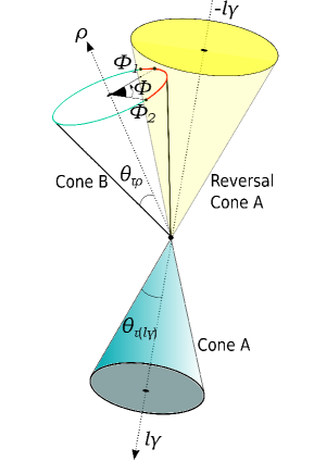
where the parameter denotes the angle along the arc
illustrated in Fig. 2.
Figure 2: Kinematics of decay.
Cones A and B are the surfaces that satisfy the c.m.s. conditions and .
The direction of is constrained to lie on an arc defined by the
intersection of cone B and the interior or exterior
sector constrained by the reversal (i.e., mirror) cone A.
The arc (shown in red) is parametrized by the angle .
The visible differential cross section is, therefore, obtained by
integration over :
(14)
(15)
(16)
where is proportional to the probability density function (PDF)
of the signal and denotes the set of twelve measured variables:
.
There are several corrections that must be incorporated in the
procedure to take into account the real experimental situation.
Physics corrections include electroweak higher-order corrections
to the cross section
[14, 15, 16, 17, 18].
Apparatus corrections include the effect of the finite detection
efficiency and resolution, the effect of the external bremsstrahlung
for events, and the beam energy
spread.
Accounting for the event-selection criteria and the contamination from
identified backgrounds, the total visible (properly normalized) PDF
for the observable in each event is given by
(17)
where
is the distribution of the category of background,
is the fraction of this background, and
is the
selection efficiency of the signal distribution.
The categorization of is explained later (see the caption
of Fig. 3).
In general, is evaluated as an integral of the background
PDF multiplied by the inefficiency that depends on the variables of missing particles.
The PDFs of the dominant background processes are described
analytically one by one, while the remaining background processes
are described by one common PDF, tabulated from Monte Carlo (MC) simulation.
The denominator of the signal term in Eq. (17)
represents normalization.
Since is a linear combination of the Michel parameters
,
the normalization of signal PDF becomes
(18)
(19)
(20)
(21)
where is a normalization coefficient of the SM part defined by
,
represents a set of variables for the
selected event of events,
is an average selection efficiency,
and the brackets indicate an average with respect
to the selected SM distribution.
We refer to and
()
as absolute and relative normalizations, respectively.
From , the negative logarithmic
likelihood function (NLL) is constructed and the best estimators of the
Michel parameters, and , are obtained by
minimizing the NLL. The efficiency is a common
multiplier in Eq. (17) and does not depend on the Michel
parameters. This is one
of the essential features of the unbinned maximum likelihood method.
We validated our fitter and procedures using a MC sample generated
according to the SM distribution.
The optimal values of the Michel parameters are consistent with their SM
expectations within the statistical uncertainties.
2.2 KEKB collider
The KEKB collider (KEK laboratory, Tsukuba, Japan) is an
energy-asymmetric collider with beam energies of 3.5 GeV and 8.0 GeV
for and , respectively.
Most of the data were taken at the c.m.s. energy of 10.58 GeV,
corresponding to the mass of the , where a huge number of
as well as pairs were produced.
The KEKB collider was operated from 1999 to 2010 and accumulated
1 of collision data with the Belle detector.
The achieved instantaneous luminosity of
is the world record.
For this reason, the KEKB collider is often called a -factory
but it is worth considering it also as a -factory,
where pair events have been produced.
The world largest sample of leptons collected at Belle provides
a unique opportunity to study radiative leptonic decay of .
In this analysis, we use 711 f of collision data
collected at the resonance energy [19].
2.3 Belle detector
The Belle detector is a large-solid-angle magnetic
spectrometer that consists of a silicon vertex detector,
a 50-layer central drift chamber (CDC), an array of
aerogel threshold Cherenkov counters (ACC), a barrel-like arrangement of time-of-flight
scintillation counters (TOF), and an electromagnetic calorimeter
comprised of CsI(Tl) crystals (ECL) located inside
a superconducting solenoid coil that provides a 1.5 T
magnetic field. An iron flux return located outside of
the coil is instrumented to detect mesons and to identify
muons (KLM). The detector
is described in detail elsewhere [20].
3 Event selection
The event selection proceeds in two stages. At the preselection,
candidates are selected efficiently while suppressing
the beam background and other physics processes like radiative Bhabha scattering,
two-photon interaction, and radiative pair production.
The preselected events are then required to satisfy final selection
criteria to enhance the purity of the signal events.
3.1 Preselection
•
There must be exactly two oppositely charged tracks in the event.
The impact parameters of these tracks relative to the interaction point
are required to be
within cm along the beam axis and cm in the transverse
plane.
The two-track transverse momentum must exceed GeV/ and that
of one track must exceed GeV/.
•
Total energy deposition in the ECL in the laboratory frame must be lower
than 9 GeV.
•
The opening angle of the two tracks must satisfy in the laboratory frame.
•
The number of photons whose energy exceeds MeV in the c.m.s. must be fewer than five.
•
For the four-vector of missing momentum defined by
,
the missing mass defined by
must lie in the range
GeV GeV,
where and
are the four-momenta of the beam and all detected particles, respectively.
•
The polar angle of missing-momentum must satisfy
in the laboratory frame.
3.2 Final selection
The candidates of the outgoing particles in
,
i.e., the lepton, photon, and charged and neutral pions,
are assigned in each of the preselected events.
•
The electron selection is based on the likelihood ratio cut, ,
where and are the likelihood values of the track for the electron
and non-electron hypotheses, respectively.
These values are determined using specific ionization
() in the CDC, the ratio of ECL energy and CDC momentum
,
the transverse shape of the cluster in the ECL, the matching
of the track with the ECL cluster, and the light yield in the
ACC [21].
The muon selection uses the likelihood ratio
, where the likelihood values are
determined by the measured versus expected range for the hypothesis,
and transverse scattering of the track in the KLM [22].
The reductions of the signal efficiencies with
lepton selections are approximately 10% and 30%
for the electron and muon, respectively.
The pion candidates are distinguished from kaons using ,
where the likelihood values are determined by the ACC response,
the timing information from the TOF, and in the CDC.
The reduction of the signal efficiency with pion selection is approximately 5%.
•
The candidate is formed from two photon candidates,
where each photon satisfies
MeV, with an invariant mass of MeV MeV.
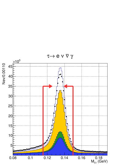
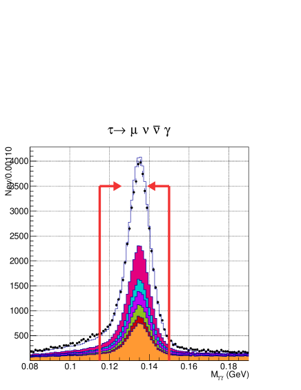
Figure 3 shows the distribution of the invariant mass
of the candidates. The reduction of the signal efficiency by the mass selection is approximately 50%.
In addition, when more than two candidates are found, the event is rejected.
•
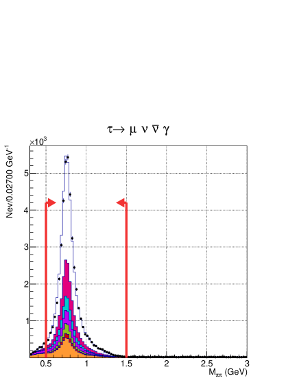
The candidate is formed from a and a candidate,
with an invariant mass of GeV.
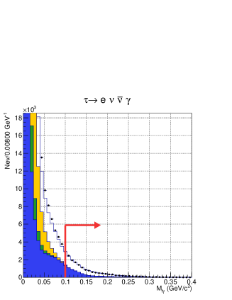
Figure 4 shows the distribution of the invariant mass of the
candidates.
The reduction of the signal efficiency is approximately 3%.
•
The c.m.s. energy of signal photon candidate must exceed MeV if
within the ECL barrel () or
MeV if within the ECL endcaps
( or ).
As shown in Fig. 5, this photon must lie in a cone determined
by the lepton-candidate direction that is defined by
cos and
cos for the electron and muon mode, respectively,
where ( or ) is the angle between the lepton and the photon.
The reductions of the signal efficiencies for the requirement
on this photon direction are approximately 11% and 27% for the
electron and muon mode, respectively.
Furthermore, if the photon candidate and either of the photons
from the , which is a daughter of the candidate,
form an invariant mass of the
( MeV MeV),
the event is rejected. The additional selection reduces the signal
efficiency by .
•
The direction of the combined momentum of the lepton and photon in
the c.m.s. must not belong to the hemisphere determined by the
candidate: an event should satisfy
, where is the spatial
angle between the system and the candidate.
This selection reduces the signal efficiency by .
•
There must be no additional photons in the aforementioned cone
around the lepton candidate; the sum of the energy in the laboratory frame
of all additional photons that are not associated
with the or the signal photon (denoted as
) should not exceed 0.2 GeV and 0.3 GeV for
the electron and muon mode, respectively. The reductions of the signal
efficiencies for the requirement
on the are approximately 14% and 6%
for the electron and muon mode, respectively.
(a)
(b)
Figure 3: Distribution of . Dots with uncertainties
are experimental data and histograms are MC distributions.
The MC histograms are scaled to the experimental one based on
the yields just after the preselection.
The red arrows indicate the selection window MeV
MeV.
(a) candidates:
the open histogram corresponds to the signal, the yellow () and
green () histograms represent ordinary leptonic decay plus extra bremsstrahlung due
to the detector material and
radiative leptonic decay plus bremsstrahlung,
respectively, and the blue () histogram represents other processes such as radiative Bhabha,
two-photon, and productions.
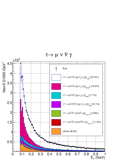
(b) candidates:
the open histogram corresponds to signal, the magenta () histogram represents
ordinary leptonic decay plus beam background,
the aqua () histogram represents ordinary leptonic decay plus ISR/FSR
processes, the purple () histogram represents three-pion events where
is misreconstructed
as a tagging candidate,
the green () histogram represents - background
where is selected due to misidentification
of pion as muon, the red () histogram represents 3- events
where is selected by
misidentification similarly to the - case, and the orange ()
histogram represents other processes (as in the electron mode).
In Eq. (17) and
the categories mentioned in this caption, and
for the electron and muon modes, respectively.
(a)
(b)
Figure 4: Distribution of :
(a) candidates and (b) candidates.
Dots with uncertainties are experimental data and histograms are MC distributions.
The color of each histogram is explained in Fig. 3.
The red arrows indicate the selection window
GeV MeV.
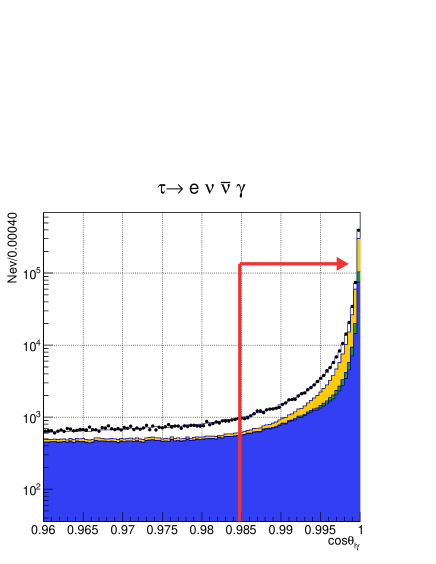
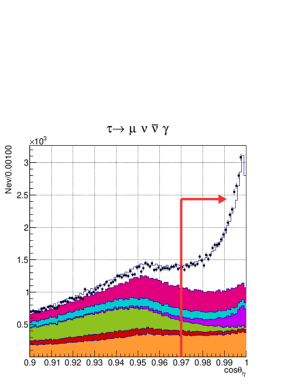
(a)
(b)
Figure 5: Distribution of :
(a) candidates and (b)
candidates.
Dots with uncertainties are experimental data and histograms are MC distributions.
The color of each histogram is explained in Fig. 3.
The red arrows indicate the selection condition cos and
cos for the electron and muon mode, respectively.
These selection criteria are optimized using MC simulation
(five times as large as real data)
where pair production and
the successive decay of the
are simulated by the KKMC [23] and
TAUOLA [24, 25]
generators, respectively. The detector effects are simulated based
on the GEANT3 package [26].
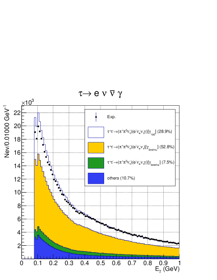
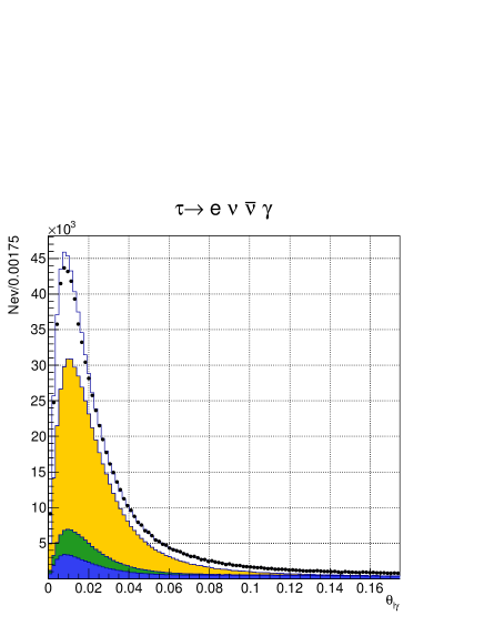
(a)
(b)
Figure 6: Final distribution of (a) photon energy and (b)
for the decay candidates.
Dots with uncertainties are experimental data and histograms
are MC distributions.
The color of each histogram is explained in Fig. 3.
(a)
(b)
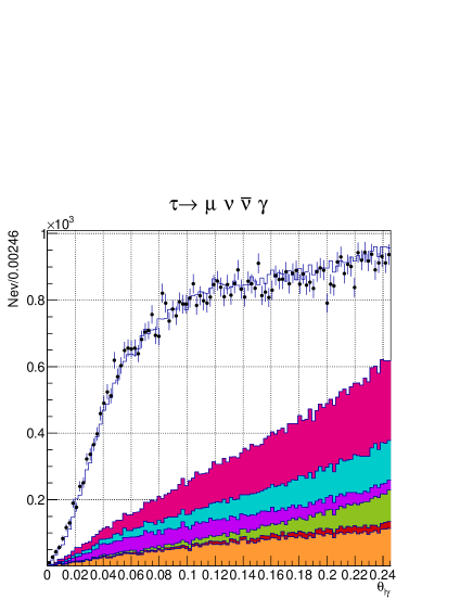
Figure 7: Final distribution of (a) photon energy
and (b) for the decay candidates.
Dots with uncertainties are experimental data and histograms are MC distributions.
The color of each histogram is explained in Fig. 3.
Distributions of the photon energy and the angle between
the lepton and photon, , for the selected events are shown
in Figs. 6 and 7 for
and
candidates, respectively.
In the electron mode, the fraction of the signal decay in the selected
sample is about due to the large external bremsstrahlung rate in
the non-radiative leptonic
decay events. In the muon mode, the
fraction of the signal decay is about ; here,
the main background arises from ordinary leptonic
decay () events
where either an additional photon is reconstructed from beam background
in the ECL or a photon is emitted by the
initial-state . The information
is summarized in Table 2.
As mentioned before, in the integration over
in Eq. (15),
the generated differential variables are varied according to the
resolution function .
Thus, the kinematic variables
can extend outside the allowed phase
space.
For the unphysical values, we assign zero to
the integrand because this implies negative neutrino masses.
If such discarded trials in the integration exceed 20% of the total
number of iterations,
we reject the event.
This happens for events that lie near the kinematical boundary
of the signal phase space.
The corresponding reduction of the efficiency is approximately
2% and 3% for the electron and muon mode, respectively.
This additional decrease of the efficiency
is not reflected in the values of Table 2.
Table 2: Summary of event selection
Item
391954
384880
35198
35973
(%)
Purity (%)
The efficiency is
determined based on the photon
energy threshold of MeV in the
rest frame.
4 Analysis of experimental data
When we fit the Michel parameters for the real experimental data,
the difference in selection efficiency between real data and MC simulation
must be taken into account by the correction factor
that is close to unity; its extraction is described below.
With this correction, Eq. (17) is modified to
(22)
The presence of in the numerator does not affect the NLL
minimization, but its presence in the denominator does.
We evaluate as the product of the measured corrections
for the trigger,
particle identification, track, , and reconstruction efficiencies:
(23)
(24)
(25)
The lepton identification efficiency correction is estimated
using two-photon processes
( or ).
Since the momentum of the lepton from
the two-photon process ranges from the detector threshold
to approximately GeV in the laboratory frame,
the efficiency correction factor
can be evaluated for our signal process
as a function of and .
The pion PID correction factor is obtained
by the measurement of
decay
(where the subscript indicates “slow”).
The small momentum of the pion from allows us to select this process.
As a result, assuming the mass of meson, we can reconstruct even if
this is missed.
The track reconstruction efficiency correction is extracted from
events.
Here, we count the number of events () in which four (three)
charged tracks are reconstructed.
The three-track event is required to have a negative net charge
( is missing).
Since the charged track reconstruction efficiency
is included as, respectively,
and in and ,
the value of can be obtained by .
The momentum and angular dependences of are
extracted by modifying , where
is the number of observed events in a certain cell of
the phase-space of reconstructed track.
The reconstruction efficiency correction is obtained by comparing
the ratio of the number
of selected events of
and between
experiment and MC simulation. The momentum
and angular dependence of the reconstruction efficiency is extracted
by counting the number of events observed in a certain kinematic-variable
cell of the phase space.
By randomly choosing either of the photon daughters from the ,
the reconstruction efficiency correction is
extracted in the same manner.
The trigger efficiency correction has the largest impact among these factors.
In particular, for the electron mode, because of the similar structure
of our signal events and Bhabha events (back-to-back topology of
two-track events),
many signal events are rejected by the Bhabha veto in the trigger.
The veto of the trigger results in a spectral distortion and a large
systematic uncertainty.
The correction factor is extracted using
the charged and neutral subtriggers (denoted as and ), which provide
completely independent signals.
Since the trigger signal appears when at least one of the subtriggers
fires (i.e., OR ), its efficiency is given by
, where
and are
the efficiencies of the charged and neutral subtriggers, respectively;
is the number of events where both subtriggers fire
(i.e. AND ), () is a number of events triggered by ().
Thus is obtained as the ratio of
between the experiment and MC simulation.
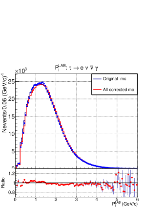
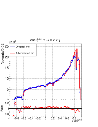
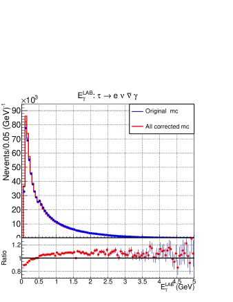
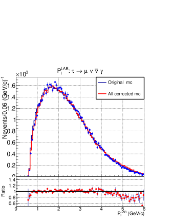
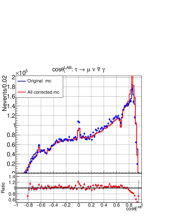
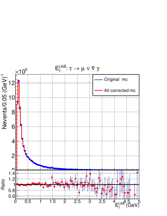
Figure 8 shows the distribution of the momentum and the
cosine of the polar angle of electron and muon events.
In the figure, the effects of all corrections are seen mainly
at cos and cos.
(a)
(b) cos
(c) ( mode)
(d)
(e) cos
(f) ( mode)
Figure 8: Distributions of momenta of leptons, cosine of angles and photon energy:
(a)(b)(c) for the electron modes and (d)(e)(f) for the muon modes.
Blue points with uncertainties represent the experimental data while
the black and red lines represent the distributions of the original
and corrected MC simulation, respectively.
5 Evaluation of systematic uncertainties
Table 3: List of systematic contributions
Item
Relative normalizations
0.13
0.04
Absolute normalizations
Formulation of PDFs
0.67
0.22
Input of branching ratio
Effect of cluster overlap in ECL
Detector resolution
0.74
0.20
0.22
0.02
Exp/MC corrections
cut
0.91
0.22
-
-
Total
6.8
0.93
0.77
0.25
In Table 3, we summarize the contributions of the identified
sources of systematic uncertainties.
The dominant source for the electron mode is the calculation of the relative normalizations.
Due to the peculiarity of the signal PDF when ,
the convergence of the relative normalization coefficients is quite
slow and results in a notable effect. For a given number of MC events ,
the errors of the relative normalizations () are
evaluated by , where represents the variance of a random variable .
The resulting systematic effect on the Michel parameter is estimated by varying the normalizations.
The effect of the absolute normalization is estimated in the same way.
The largest systematic uncertainty for the muon mode is due to the limited precision of the description
of the background PDF that appears in Eq. (22).
As mentioned before, the remaining background sources are described
by a common PDF, which is tabulated utilizing a large generic MC sample.
This effective description can generally discard information about correlations
in the phase space and thereby give significant bias.
The residuals of the fitted Michel parameters from the SM prediction obtained by the fit to the MC distribution
are taken as the corresponding systematic uncertainties.
Other notable uncertainties come from the accuracy of the
measured branching ratios.
In particular, the uncertainties of the branching ratio of the radiative
decay dominate the contribution.
The systematic effects of the cluster merging in the ECL are evaluated as a function of the
angle between the photon and lepton clusters at the front face of ECL ().
The limit represents the merger of the two clusters
and the comparison of the distribution between experiment and MC gives us the corresponding bias.
A systematic effect due to the detector resolution is evaluated by comparing Michel parameters
obtained in the fit with and without account
of the resolution function .
The error of the measured correction factor is estimated by varying the central
values based on the uncertainty in each bin.
Moreover, as can be observed in Fig. 8d in the muon mode,
there is a notable disagreement of efficiency in the forward domain (cos).
This is due to the contamination of backgrounds in the extraction of the correction factor
of .
We excluded this region (reducing the statistics by 1.5%) and
checked the shift of the refitted Michel parameters.
In the electron mode, we observe the disagreement
of the photon reconstruction efficiency
in the low-energy region (Fig. 8c).
It could arise from a discrepancy in the simulation of extra bremsstrahlung.
We excluded the events having a low energy photon MeV and
compared the refitted values. Because this cut reduces the number of events
by approximately 20%, the statistical fluctuation is also
reflected in the shifts.
The effect of the beam-energy spread is estimated by varying the input of this
value for the calculation of the PDF with respect to run-dependent uncertainties, and
turns out to be negligible.
The effects from the next-to-leading-order (NLO) contribution were checked
by adding the NLO formulae [27] to the signal PDF and refitting, and
were found to be negligible.
6 Results
Because of the suppression of sensitivity due to the small mass of the electron,
the parameter is extracted only from the mode.
Using the 71171 selected candidates,
and are simultaneously fitted to the kinematic distribution to be
(26)
(27)
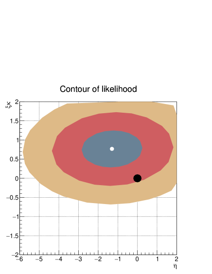
Figure 9 shows the contour of the likelihood
function for events.
Figure 9: Contours of the likelihood function obtained using 71171
events for candidates.
The ovals are 1-, 2- and 3-contours of statistical deviation of the likelihood function from the best estimation.
The black dot is the SM prediction.
In the electron mode, is fitted by fixing the value to the
SM prediction of and the optimal value is extracted using 776834 events to be
(28)
In Equations 26–29, the first error is statistical and second systematic.
The obtained values are consistent with the SM prediction.
Furthermore, the product is
also obtained by fitting simultaneously to both electron and muon events as
(29)
Here, the systematic uncertainty
is estimated from
by assuming they are uncorrelated.
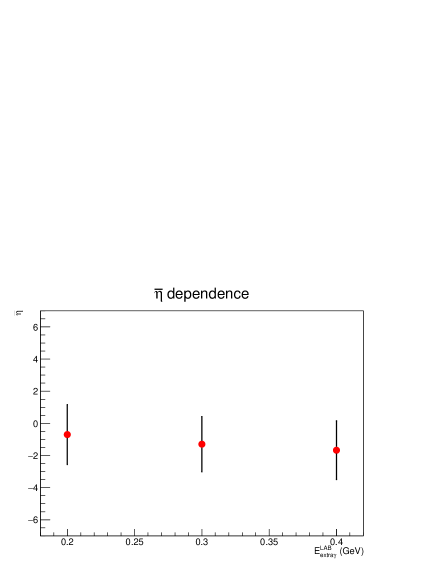
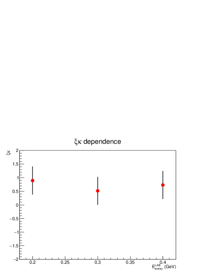
We also obtain the dependence of the
selection on the fitted Michel parameters as shown in Fig. 10.
In the extraction of , we use
while, for , we use the combined
result for
and decays.
We observe stability of the fitted Michel parameters within uncertainties.
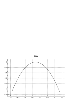
Figure 11 shows the residual of the likelihood function
projected onto one axis.
We observe a smooth and quadratic shape of the NLL around its minimum.
(a)
(b)
Figure 10: Dependence of Michel parameters on
the selection (a) (b) and .
The red markers with bars correspond to the optimal values of Michel parameters
and their uncertainties, where both statistical and systematic uncertainties
are considered.
(a)
(b)
(c)
Figure 11: Plot of as a function of Michel parameters; (a) when
is set to the fitted value;
(b) when ;
(c) when is set to the fitted value.
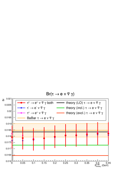
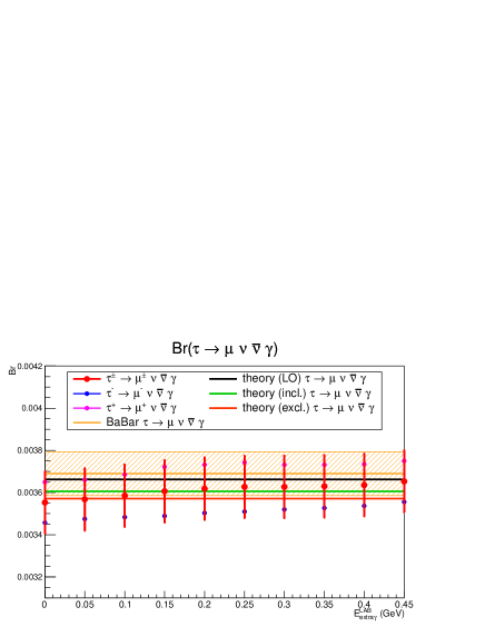
7 Measurement of the branching ratio
In addition to the Michel parameters, we have determined the
branching ratios of the
() decays.
Following the definition of Ref. [27], we distinguish
between two types of radiative decays in the NLO approximation:
the exclusive radiative decay implies that only one hard photon is emitted in
the event; in the inclusive radiative decay, at least one hard photon
is emitted. Here, the hard photon energy threshold is 10 MeV in the
rest frame.
In Ref. [27],
the precision measurement of the branching ratios of the radiative
leptonic decays at BaBar is also discussed.
While the measured branching ratios of both electron and muon modes agree
with their leading-order (LO) theoretical predictions,
the NLO exclusive branching ratio prediction for the
decay differs from
the BaBar result by 3.5 standard deviations.
This is explained by the insufficient accuracy of the current
MC simulation of the radiative and doubly-radiative leptonic
decays.
Neither an NLO correction to the radiative leptonic decay, nor the
doubly-radiative leptonic mode itself,
are incorporated in the current version of the TAUOLA MC generator.
As a result, the detection efficiency is not precisely evaluated for the
radiative decay. As well, the background from the doubly
radiative decay
is not subtracted at all. Finally, the second photon emission might
affect the efficiency of the photon veto and the shape of the neutral clusters
in the calorimeter. Indeed, the ratio of the yield with two-photon
emission to that with single-photon emission is approximately
5% and 1% for the electron and muon modes, respectively. Thus, there is an
experimentally notable impact of the two-photon emission on the electron mode.
In our measurement of the branching ratios, we do not take into account
the up-to-date formalism of Ref. [27] since
the main purpose of this study is a consistency check of our selection
criteria and experimental efficiency corrections.
7.1 Method
The branching ratio is determined using
(30)
where [11]
is the branching ratio of decay,
is the number of observed events, is the
fraction of background events,
is the cross section of the
process at [28],
is the integrated luminosity recorded at , and
is the average detection efficiency of signal events.
The efficiency, , is evaluated with help of the MC simulation.
The correction factor, ,
which is used to extract Michel parameters, is applied to compensate for the difference between experimental
and MC efficiencies as follows:
(31)
where is the PDF of the signal events and is
an average efficiency correction factor for the selected signal MC events.
Here, the average MC efficiency, , is
determined for the photon energy threshold of MeV in the rest frame.
7.2 Event selection
We apply additional selection criteria to enhance the purity of the sample
as well as to reduce systematic uncertainties.
The extra-gamma-energy selection is released for the latter purpose but other
selection criteria are common to those of Michel parameter measurement (see in Sec. 3).
For the electron mode, we apply the following selection criteria:
•
The uncertainty of the lepton identification efficiency in the forward
and backward regions of the detector is large due to the notable background
contamination of the control sample; thus,
the electron polar angle in the laboratory frame must lie in the region defined by
as shown in Figs. 12a and 12b.
•
The electron identification is less precise at small momenta,
so we apply the momentum threshold as shown in Fig. 12c.
•
After the final selections (explained in Sec. 3),
the dominant background arises from the external bremsstrahlung on the material of the
detector. It is effectively suppressed by applying the requirement on the invariant mass
of the electron-photon system, , as shown in Fig. 13.
•
The extra gamma energy in the laboratory frame, ,
must be less than GeV.
For the muon mode, we apply the following selection criteria:
•
The muon polar angle in the laboratory frame must satisfy
.
•
The spatial angle between and in c.m.s. must satisfy .
•
The extra gamma energy in laboratory frame, , must be smaller
than GeV.
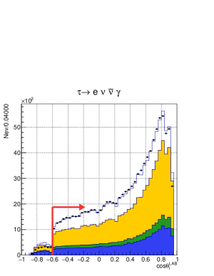
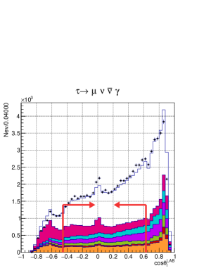
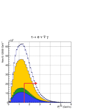
(a) cos
(b) cos
(c)
Figure 12: Cosine of the polar angle for the electron (a) and muon (b) modes, and momentum of electron (c).
The color of each histogram is explained in the caption of Fig. 3 and the red arrows indicate the selection windows:
(a) , (b)
and (c) GeV. The relative drop of the efficiencies are approximately 2%, 50% and 36%
for (a), (b), and (c), respectively. The small peak around seen in (b) comes from the
beam background.
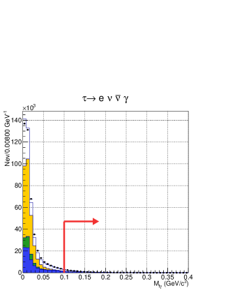
(a)
(b)
Figure 13: Distribution of the invariant mass of system, .
The color of each histogram is explained in Fig. 3 and the red arrows indicate
the selection windows. (a) overall view (b) enlarged view. The relative decrease of the
efficiency is 93%.
7.3 Evaluation of systematic uncertainties
In Table 4, we summarize the sources of the systematic uncertainties of the branching ratios
of the electron and muon modes. To estimate a systematic uncertainty from the efficiency correction, ,
we use the following method. The uncertainties of the are
determined by the finite statistics of sample,
a comparison of from and
from , and its time variation during the experiment.
values are estimated from the finite statistics of a sample,
the fit of the reconstructed mass distribution of , and observation of time variation.
The systematic uncertainties of the
, ,
, and values are estimated
from a comparison between and unity.
The uncertainty of
is taken from the PDG average value [11]
and that of is taken from
Ref. [28].
The statistical uncertainty of MC events is ignored because
its fluctuation is small.
The evaluation of the systematic uncertainty of the purity is
estimated based on sideband information.
The sideband events are selected by the following criteria:
GeV and cos for the
electron (muon) mode,
where other selection criteria are common with those of the signal extraction.
The difference of the background yield in the sideband region between
MC simulation and the real experiment
is (5.5%) for the electron (muon) mode.
Taking each fraction into account, we estimate that the resulting uncertainty is
and .
The effect of detector response is estimated
by varying selection cut parameters.
The effect due to variation of the photon energy threshold is
based on the energy resolution at the threshold, and found to be 5% [20].
The variation of other selection criteria is determined based on the
propagation of the error matrix of the helix parameters.
Of all the selection criteria, the requirement of
GeV has the largest impact.
As mentioned, to estimate the efficiency, we define the radiative events by
the imposition of a photon energy threshold of MeV
in the rest frame.
However, in the real experiment, we
cannot precisely determine this energy because the
momentum
is not directly reconstructed.
Accordingly, there is a chance that an event that has a photon
with an energy less than the threshold is also reconstructed
as signal. This is only possible in a limited phase space, and
such events are included in the selection with fractions of
and
for electron and muon events, respectively.
We take these fractions as sources of systematic effects due to
the uncertainty of the experimental threshold.
Table 4:
Systematic uncertainties (%)
on
for different configurations.
Item
Purity
1.3
1.3
Detector response
1.5
1.5
0.6
0.6
Uncertainty of threshold
1.1
1.1
0.3
0.3
Luminosity
Total
7.4 Result
In Table 5, we show the result of measurements separately
for the four following configurations:
, ,
and .
They are combined to give
(32)
(33)
where the first error is statistical and the second is systematic.
In Table 6, we summarize the current experimental and theoretical
information on these decays.
While the LO theoretical calculations for these decays
were done long time ago, NLO corrections were
considered thoroughly only recently in Ref. [27],
where the importance of taking into account the hard doubly-radiative decays
was emphasized.
We also obtain the dependence of Michel parameters on the
selection, as shown in Fig. 14.
These results are consistent with the LO theoretical prediction.
Table 5: Summary of results for the branching ratio measurement
Item
()
()
()
Table 6: Information on the branching ratios of the radiative leptonic
decays.
Figure 14: Branching ratio of
decay as a function
of cut: (a) and (b) .
Red, blue, and magenta lines represent the measured branching ratio of
, and
, respectively.
The bars represent uncertainties and are drawn only for the combined modes, where both statistical and systematic uncertainties are included.
The orange band shows the BaBar measurement [30].
Black, green, and red lines are LO, NLO inclusive, and NLO exclusive
theoretical predictions, respectively [27].
As summarized in Table 4,
the dominant systematic contribution comes from
the uncertainty of the efficiency correction for .
This uncertainty is canceled when
we measure the ratio of branching fractions
.
Moreover, other common systematic sources, namely , , the integrated luminosity,
the branching ratio of decay, and
the cross section , also cancel.
The obtained ratio is
(34)
where the first error is statistical and the second is systematic.
In Table 7, we summarize the theoretical prediction and past experimental results
for the ratio .
†Systematic uncertainty is calculated from the reference
values, where cancellation is not taken into account.
The statistical and systematic uncertainties are combined for
the CLEO and BaBar measurements.
8 Conclusion
We present the measurement of Michel parameters and of
the using 711 f of data collected with the Belle detector at the KEKB collider.
These parameters are extracted from the radiative leptonic decay
which is tagged by decay of the partner
to exploit the spin-spin correlation in .
Due to the small sensitivity to in the electron mode,
this parameter is extracted only from
to give .
The product is measured using both decays ( and )
to be . The first error is statistical and the second
is systematic. This is the first measurement of both parameters for the lepton.
These values are consistent with the SM expectation within uncertainty.
For a consistency check of the procedure to measure the Michel
parameters, we measure the branching ratio of
decay.
The obtained values are consistent with the LO theoretical
prediction and support the measurement by BaBar, which is known to
deviate from the SM exclusive branching ratio by 3.5.
Accounting for the agreement between our result and the BaBar measurement [30], the implementation
of the NLO formalism in the TAUOLA generator is required to carry out more precise measurements.
References
[1] L. Michel, Proc. Phys. Soc. A 63, 514 (1950).
[2] C. Bouchiat and L. Michel, Phys. Rev. 106, 170 (1957).
[3]W. Fetscher, H. J. Gerber and K. F. Johnson, Phys. Lett. B173, 102 (1986).
[4] W. Fetscher and H. J. Gerber, Adv. Ser. Direct. High Energy Phys. 14, 657 (1995).
[5] M. Fael, L. Mercolli and M. Passera, Phys. Rev. D88, 093011 (2013).
[6] C. Fronsdal and H. Uberall, Phys. Rev. 113, 654 (1939).
[7]A. B. Arbuzov and T.V. Kopylova, JHEP. 1609, 109 (2016).
[8] Y. S. Tsai, Phys. Rev. D4, 2821 (1971).
[9] W. Fetscher and H. J. Gerber, ETH-IMP PR-93-1 (1993).
[10] A. Stahl and H. Voss, Z. Phys. C74, 73 (1997).
[11] K.A. Olive et al. (Particle Data Group), Chin. Phys. C38, 090001 (2014).
[12] A. Heister et al. (ALEPH Collaboration), Eur. Phys. J. C22, 217 (2001).
[13] J. P. Alexander et al. (CLEO Collaboration), Phys. Rev. D56, 5320 (1997).
[14] A. B. Arbuzov et al.,
JHEP 9710, 001 (1997).
[15] E. A. Kuraev and V. S. Fadin,
Sov. J. Nucl. Phys. 41, 466 (1985), [Yad. Fiz. 41 733 (1985)].
[16] F. A. Berends et al.,
Acta Phys. Polon. B 14, 413 (1983).
[17] S. Jadach and Z. Wa̧s,
Acta Phys. Polon. B 15 1151 (1984), [Erratum B 16 483 (1985)].
[18] S. Jadach and Z. Wa̧s,
Comput. Phys. Commun. 36, 191 (1985).
[19] S. Kurokawa and E. Kikutani, Nucl. Instrum. Methods Phys. Res. Sect.
A 499, 1 (2003), and other papers included in this Volume.
T. Abe et al., Prog. Theor. Exp. Phys. 2013, 03A001 (2013)
and references therein.
[20]A. Abashian et al. (Belle Collaboration), Nucl. Instrum. Methods
Phys. Res. Sect. A 479, 117 (2002); also see detector section in
J. Brodzicka et al., Prog. Theor. Exp. Phys. 2012, 04D001 (2012).
[21] K. Hanagaki et al., Nucl. Instrum. Meth. A485, 490 (2002).
[22] A. Abashian et al., Nucl. Instrum. Meth. A491, 69 (2002).
[23] S. Jadach, B.F.L. Ward, and Z. Wa̧s, Comput. Phys. Commun. 130, 260 (2000).
[24] Z. Wa̧s, Nucl. Phys. Proc. Suppl. 98, 96 (2001).
[25] S. Jadach and Z. Wa̧s, Comput. Phys. Commun. 76, 361 (1993).
[26] R. Brun et al., CERN-DD-78-2 (1978).
[27] M. Fael et al., JHEP. 07. 153 J (2015).
[28] S. Banerjee et al., Phys. Rev. D77, 054012 (2008).
[29] T. Bergfeld et al. (CLEO Collaboration), Phys. Rev. Lett. 84, 830 (2000).
[30] J. P. Lees et al. (BaBar Collaboration), Phys. Rev. D 91, 051103 (2015).
Acknowledgments
We would like to express our deepest appreciation to
A.Arbuzov, M.Fael, T.Kopylova, L.Mercolli and M.Passera
for very useful discussions and theoretical support of this work.
We thank the KEKB group for the excellent operation of the
accelerator; the KEK cryogenics group for the efficient
operation of the solenoid; and the KEK computer group,
the National Institute of Informatics, and the
PNNL/EMSL computing group for valuable computing
and SINET5 network support. We acknowledge support from
the Ministry of Education, Culture, Sports, Science, and
Technology (MEXT) of Japan, the Japan Society for the
Promotion of Science (JSPS), and the Tau-Lepton Physics
Research Center of Nagoya University;
the Australian Research Council;
Austrian Science Fund under Grant No. P 26794-N20;
the National Natural Science Foundation of China under Contracts
No. 10575109, No. 10775142, No. 10875115, No. 11175187, No. 11475187,
No. 11521505 and No. 11575017;
the Chinese Academy of Science Center for Excellence in Particle Physics;
the Ministry of Education, Youth and Sports of the Czech
Republic under Contract No. LTT17020;
the Carl Zeiss Foundation, the Deutsche Forschungsgemeinschaft, the
Excellence Cluster Universe, and the VolkswagenStiftung;
the Department of Science and Technology of India;
the Istituto Nazionale di Fisica Nucleare of Italy;
the WCU program of the Ministry of Education, National Research Foundation (NRF)
of Korea Grants No. 2011-0029457, No. 2012-0008143,
No. 2014R1A2A2A01005286,
No. 2014R1A2A2A01002734, No. 2015R1A2A2A01003280,
No. 2015H1A2A1033649, No. 2016R1D1A1B01010135, No. 2016K1A3A7A09005603, No. 2016K1A3A7A09005604, No. 2016R1D1A1B02012900,
No. 2016K1A3A7A09005606, No. NRF-2013K1A3A7A06056592;
the Brain Korea 21-Plus program, Radiation Science Research Institute, Foreign Large-size Research Facility Application Supporting project and the Global Science Experimental Data Hub Center of the Korea Institute of Science and Technology Information;
the Polish Ministry of Science and Higher Education and
the National Science Center;
the Ministry of Education and Science of the Russian Federation and
the Russian Foundation for Basic Research;
the Slovenian Research Agency;
Ikerbasque, Basque Foundation for Science and
MINECO (Juan de la Cierva), Spain;
the Swiss National Science Foundation;
the Ministry of Education and the Ministry of Science and Technology of Taiwan;
and the U.S. Department of Energy and the National Science Foundation.
Appendix A: Differential decay width of
The general differential cross section of decay is expressed
as a sum of the two terms:
(35)
where and represent spin-independent and spin-dependent terms, () is
the energy in the rest frame and () is the
solid
angle defined by ().
These terms are functions of dimensionless kinematic parameters and defined as
(36)
(37)
(38)
(39)
(40)
and are parametrized by the Michel parameters , , , , , , and .
(41)
(42)
where and are normalized directions of lepton and photon in the rest frame,
respectively, and is a velocity of daughter lepton in this frame.
The , and () are functions of , , , and and their explicit formulae are given in the
Appendix of Ref. [7].
Appendix B: Differential decay width of
We use the CLEO model to define the differential decay width of decay.
This is expressed as a sum of the spin-independent and spin-dependent parts [13]:
(43)
(44)
(45)
where is the corresponding element of the Cabibbo-Kobayashi-Maskawa matrix,
and () are energies and three-momenta measured in the rest frame,
is
the solid angle of the meson in the rest frame, is the solid angle of the pion in the rest frame,
is a four-momentum defined by , and is the four-momentum of the
tau neutrino.
The factor BPS stands for the square of a relativistic Breit-Wigner function and a Lorentz-invariant phase space, and is calculated as follows:
(46)
(47)
(48)
(49)
(50)
The factor ( or ) represents the Breit-Wigner function associated with the
resonance mass shape, and the parameter specifies their relative coupling.
The nominal masses of the two resonance states are
and , and their nominal total decay widths are
and .