Two-Dimensional Molecular Gas and ongoing star formation around H II region Sh2-104

Abstract

We performed a multiwavelength study towards H II region Sh2-104. New maps of ¹²CO $J$=1-0 and ¹³CO $J$=1-0 were obtained from the Purple Mountain Observatory (PMO) 13.7 m radio telescope. Sh2-104 displays a double-ring structure. The outer ring with a radius of 4.4 pc is dominated by 12 $\mu$m, 500 $\mu$m, ¹²CO $J$=1-0, and ¹³CO $J$=1-0 emission, while the inner ring with a radius of 2.9 pc is dominated by 22 $\mu$m and 21 cm emission. We did not detect CO emission inside the outer ring. The north-east portion of the outer ring is blueshifted, while the south-west portion is redshifted. The present observations have provided evidence that the collected outer ring around Sh2-104 is a two-dimensional structure. From the column density map constructed by the Hi-GAL survey data, we extract 21 clumps. About 90% of all the clumps will form low-mass stars. A power-law fit to the clumps yields $M=281M_{\odot}(r/\rm pc)^{1.31\pm 0.08}$. The selected YSOs are associated with the collected material on the edge of Sh2-104. The derived dynamical age of Sh2-104 is 1.6$\times 10^{6}$ yr. Compared the Sh2-104 dynamical age with the YSOs timescale and the fragmentation time of the molecular ring, we further confirm that collect-and-collapse process operates in this region, indicating a positive feedback from a massive star for surrounding gas.

1 Introduction

OB stars emit copious ultraviolet (UV) photons. The UV photons with energies above 13.6 eV can ionize hydrogen to create an H II region. Since the gas pressure inside HII regions is higher than that of their surrounding neutral medium, the H II regions expand. Expanding H II regions will also reshape their surrounding molecular gas, and thereby regulate star formation in the molecular gas. Accordingly, it will brings two aspect of roles. One is the destructive role, which can evaporate or disperse the surrounding molecular gas and consequently may terminate star formation, and another is the constructive role, which can trigger star formation.

At present two main processes have been put forward for triggering star formation at the peripheries of H II regions: collect and collapse (CC) and radiation-driven implosion (RDI) (Elmegreen & Lada, 1977; Deharveng et al., 2010). In the CC process, a compressed layer of neutral material is accumulated between the ionization front and shock front, and star formation occurs when this layer becomes gravitationally unstable. Unlike the CC precess, the RDI process that a pre-existing denser gas is compressed by the shocks, and then form stars. Howerver, the CC process is more attractive because it allows the formation of massive stars or clusters (Deharveng et al., 2005). To investigate the triggered star formation by the CC process, several individual H II regions have been well studied, such as Sh-104 (Deharveng et al., 2003), RCW 79 (Zavagno et al., 2006), RCW 120 (Zavagno et al., 2007), Sh2-212 (Deharveng et al., 2008), Sh2-217 (Brand et al., 2011), Sh2-90 (Samal et al., 2014), Sh2-87 (Xu & Ju, 2014), N6 (Yuan et al., 2014) and Gum 31 (Duronea et al., 2015). Moreover, there are also some statistical studies for infrared bubbles (e.g., Deharveng et al., 2010; Kendrew et al., 2012; Thompson et al., 2012; Kendrew et al., 2016), which are created by the expanding H II regions. A common feature of the above studies that several massive fragments are found on the border of each H II region. Some star formation activities have been detected in these fragments, such as outflow, UCHII, and water masers. Generally, if an expanding H II region collect their surrounding gas, the morphology of the molecular gas will show three-dimensional spherical structure. CO observations can provide velocity information to reveal the gas structure surrounded H II regions. Beaumont & Williams (2010) observed 43 infrared bubbles using CO molecular line, but they did not detect the front and back faces of these shells at blueshifted and redshifted velocities. Hence, they concluded that the bubbles enclosing H II regions are two-dimensional rings formed in parental molecular clouds with thicknesses not greater than the bubble sizes. However, the molecular gas with a three-dimensional spherical structure or a two-dimensional ring around H II region is important for understanding the triggered star formation (Deharveng et al., 2015).

Sh2-104 is an optically visible Galactic H II region with a 7^′ diameter. The distance to Sh2-104 is $\sim$4 kpc (Deharveng et al., 2003). This H II region is excited by an O6V center star (Crampton et al., 1978; Lahulla, 1985), whose ionized gas has a LSR velocity of 0 ${\rm km~{}s}^{-1}$ (Georgelin et al., 1973). Sh2-104 displays a shell-like morphology, detected at optical and radio wavelengths. Using the Herschel data, Rodón et al. (2010) found that the dust temperature is $\sim$25 K in the photodissociation region (PDR) of Sh2-104, while it is $\sim$40 K in its interior. Deharveng et al. (2003) detected a molecular shell with four large molecular condensations around Sh2-104. An UCHII region lies at an eastern condensation, which is associated with IRAS 20160+3636. High CN/HCN ratio in the eastern condensation suggests that the condensation is affected by Sh2-104 (Minh et al., 2014). A near-IR cluster lies in the UCHII direction (Deharveng et al., 2003). The massive condensations and cluster around Sh2-104 suggests that this H II region is a typical candidate for triggering star formation by CC process.

In this paper, we performed a multi-wavelength study to further investigate the gas structure and star formation around H II region Sh2-104. The molecular gas associated with Sh 104 was observed in ¹²CO $J$=2-1, ¹³CO $J$=1-0, and C¹⁸O $J$=1-0 with the IRAM 30m telescope (Deharveng et al., 2003). Howerver, they did not give the maps of the ¹³CO $J$=1-0 and C¹⁸O $J$=1-0 molecular gas in their paper. New maps of ¹²CO $J$=1-0 and ¹³CO $J$=1-0 were shown from the Purple Mountain Observatory (PMO) 13.7m radio telescope. Combining our data with those obtained by the NRAO VLA Sky survey, the Hi-GAL survey, and the WISE survey, our aim was to construct a comprehensive large-scale picture of Sh2-104. Our observations and data reduction are described in Sect.2.1, and the results are presented in Sect.3. In Sect.4, we discuss the gas structure around Sh2-104 and star formation scenario, while our conclusions are summarized in Sect.5.

2 Observation and data processing

2.1 Archival data

We used far-infrared data (70 $\mu$m $\sim$ 500 $\mu$m) from the Herschel Infrared Galactic Plane survey (Hi-GAL; Molinari et al., 2010) carried out by the Herschel Space Observatory. The initial survey covered a Galactic longitude region of 300^∘$<$$\ell$$<$60^∘ and $|b|$$<$1.0^∘. The Hi-GAL survey used two instruments: PACS (Poglitsch et al., 2010) and SPIRE (Griffin et al., 2010) in paralel mode to carry out a survey of the inner Galaxy in five bands: 70, 160, 250, 350 and 500 $\mu$m. The scan speeds of PACS is 20^′′ per second, while 30^′′ per second for SPIRE. The angular resolutions of these five bands are 10$\farcs 7$, 11$\farcs 4$, 18$\farcs 2$, 24$\farcs 9$, and 36$\farcs 3$, respectively. These Hi-GAL data have been used to explore the flux density distribution and to construct column density map of the studied region.

The 1.4 GHz radio continuum emission data were obtained from the NRAO VLA Sky Survey (NVSS; Condon et al., 1998) which is a 1.4 GHz continuum survey covering the entire sky north of -40^∘ declination with a noise of about 0.45 mJy/beam and a resolution of 45^′′.

We also utilized infrared data from the survey of the Wide-field Infrared Survey Explorer (WISE; Wright et al., 2010). The WISE survey is mapping the whole sky in four infrared bands 3.4 $\mu$m (W1), 4.6 $\mu$m (W2), 12 $\mu$m (W3), and 22 $\mu$m (W4) at angular resolutions of 6$\farcs 1$, 6$\farcs 4$, 6$\farcs 5$, and 12^′′, respectively.

2.2 Purple Mountain Data

We also made the mapping observations of H II region Sh2-104 and its adjacent region in the transitions of ¹²CO $J$=1-0, ¹³CO $J$=1-0 and C¹⁸O $J$=1-0 lines using the Purple Mountain Observation (PMO) 13.7 m radio telescope at De Ling Ha in the west of China at an altitude of 3200 meters, during December 2016. The 3$\times$3 beam array receiver system in single-sideband (SSB) mode was used as front end. The back end is a fast Fourier transform spectrometer (FFTS) of 16384 channels with a bandwidth of 1 GHz, corresponding to a velocity resolution of 0.16 km s^-1 for ¹²CO $J$=1-0, and 0.17 km s^-1 for ¹³CO $J$=1-0 and C¹⁸O $J$=1-0. ¹²CO $J$=1-0 was observed at upper sideband with a system noise temperature (Tsys) of 272 K, while ¹³CO $J$=1-0 and C¹⁸O $J$=1-0 were observed simultaneously at lower sideband with a system noise temperature of 145 K. The half-power beam width (HPBW) was 53^′′ at 115 GHz and the main beam efficiency was 0.5. The pointing accuracy of the telescope was better than 5^′′, which was derived from continuum observations of planets (Venus, Jupiter, and Saturn). The source W51D (19.2 K) was observed once per hour as flux calibrator. The mean rms noise level of the calibrated brightness temperature was 0.4 K for ¹²CO $J$=1-0, while 0.2 K for ¹³CO $J$=1-0 and C¹⁸O $J$=1-0. Mapping observations were centered at RA(J2000)=$20^{\rm h}17^{\rm m}45^{\rm s}$, DEC(J2000)=$36^{\circ}46^{\prime}00^{\prime\prime}$ using the on-the-fly mode with a constant integration time of 14 second at each point. The total mapping area is $20^{\prime}\times 20^{\prime}$ in ¹²CO $J$=1-0, ¹³CO $J$=1-0, and C¹⁸O $J$=1-0 with a $0.5^{\prime}\times 0.5^{\prime}$ grid. The standard chopper wheel calibration technique is used to measure antenna temperature $T_{\rm A}^{\ast}$ corrected for atmospheric absorption (Kutner & Ulich, 1981). The final data was recorded in brightness temperature scale of $T_{\rm mb}$ (K). The data were reduced using the GILDAS/CLASS package.

3 Results

3.1 Infrared and Radio Continuum Images

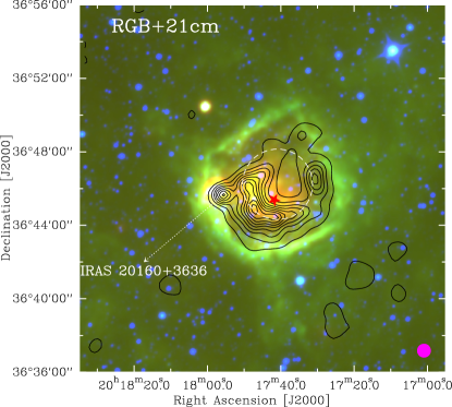
Figure 1: 1.4 GHz radio continuum contours in black colour, overlaid on the three color image of H II Sh2-104 composed from the WISE 3.4 $\mu$m, 12 $\mu$m, and 22 $\mu$m bands in blue, green, and red, respectively. The black contours begin at 5$\sigma$ in steps of 10$\sigma$, with 1$\sigma$ = 0.7 mJy beam^-1. The white dashed circle indicates an ionized gas ring for Sh2-104. The red ”star” marks the position of the exciting star.

Figure 1 shows composite three-color image of Sh2-104. The three infrared bands are the WISE 3.4 $\mu$m (in blue), 12 $\mu$m (in green), and 22 $\mu$m (in red). The WISE 12 $\mu$m band contains polycyclic aromatic hydrocarbon (PAH) emission at 11.2 $\mu$m and 12.7 $\mu$m (Tielens, 2008). The PAH molecules are excited by the UV radiation from H II region, but are easily destroyed inside ionized region. Hence, the WISE 12 $\mu$m similar to the Spitzer IRAC 8.0 $\mu$m can be used to trace PDR, and delineate H II region boundaries (Pomarés et al., 2009). In Fig. 1, the PAH emission shows a ring-like structure with an opening towards the north. For H II region, the WISE 22 $\mu$m emission traces heated small dust grains, which is similar to the MIPS 24 $\mu$m band (Anderson et al., 2014). The hot dust emission in Fig. 1 displays two sources, one related to Sh2-104, and the other associated with IRAS 20160+3636.

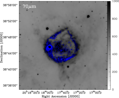
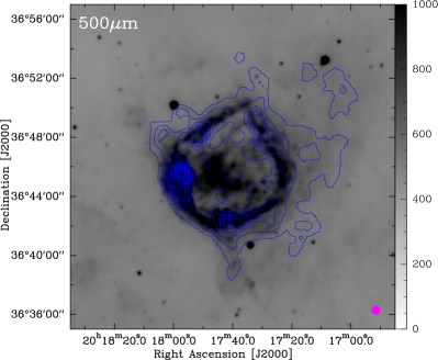
Figure 2: The Herschel 70 $\mu$m and 500 $\mu$m emission maps superimposed on the WISE 12 $\mu$m emission (grey), respectively. The units for each colour bar are Jy pixel^-1.

The NVSS 20 cm radio continuum emission can be used to trace ionized gas, which is also overlaid in Fig. 1 by black contours. The ionized gas emission in Fig. 1 indicates that Sh2-104 is a shell-like H II region, whose radius is about 2.5^′, marked by a white dashed circle. Moreover, the ionized gas emission are spatially coincident with the hot dust emission observed at the WISE 22 $\mu$m (red color). Both the ionized gas and hot dust emission are enclosed by the PAH emission. Extending towards the east, an UCHII region is located at the eastern border of Sh2-104, which is related to source IRAS 20160+3636.

The 70 $\mu$m emission is mostly produced by relatively hot dust (Faimali et al., 2012), and partly corresponds to cool dust emission (Anderson et al., 2012). Figure 2 (left panel) is the 70 $\mu$m emission map, overlaid with the WISE 12 $\mu$m emission. The 70 $\mu$m emission also displays the ring-like shape. The ring may represent the cool dust emission, which is spatially associated with the PAH emission. Inside the ring, there is an arc-like structure. From Figures 1 and 2 (left), it is seen that the arc is spatially coincident with the 20 cm radio continuum emission, indicating that this part of the 70 $\mu$m emission is producted from the hot dust. The 500 $\mu$m emission originates from cool dust with an average temperature of 26 K along the PDR (Anderson et al., 2012). Figure 2 (right panel) shows the 500 $\mu$m emission map superimposed on the WISE 12 $\mu$m emission. The 500 $\mu$m emission also shows the ring-like structure. Comparing with the 12 $\mu$m and 70 $\mu$m emission ring, it becomes more extended from the 500 $\mu$m emission. In Fig.2 (right panel), the cool dust is mainly concentrated in four large dust clumps, which are regularly distributed at the ring-like structure around Sh2-104.

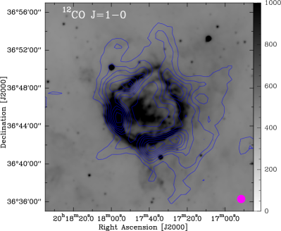
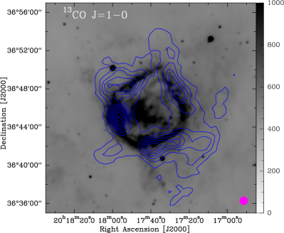
Figure 3: Left panel: Contours of ¹²CO $J$=1-0 emission superimposed on the 12 $\mu$m emission map (grey). The integrated velocity is from -3.4 to 4.2 km s^-1. The blue contour levels are from 14.7 (3$\sigma$) to 66.2 by a step of 7.3 K km s^-1 . Right panel: Contours of ¹³CO $J$=1-0 emission superimposed on the 8 $\mu$m emission map (grey). The blue contour levels are from 1.8 (3$\sigma$) to 16.2 by a step of 1.8 K km s^-1.

3.2 CO Molecular Emission

Compared with dust continuum emission, CO emission with velocity information can be used to separate whether the projected molecular gas is associated with H II region. To analyze the morphology of molecular gas consistent with H II region Sh2-104, here we use ¹²CO $J$=1-0, ¹³CO $J$=1-0, and C¹⁸O $J$=1-0 lines to trace the molecular gas. The C¹⁸O $J$=1-0 emission was detected in some points with strong ¹³CO $J$=1-0 emission, suggesting that these positions are more dense. Since the C¹⁸O $J$=1-0 signal is so week that we do not examine its spatial distribution. Comparing the optically thick ¹²CO line, the ¹³CO line is more suited to trace relatively dense gas. Using channel maps of ¹³CO line, we inspect gas component for our studied region. Georgelin et al. (1973) found that the LSR velocity of the ionized gas for Sh2-104 is about 0 ${\rm km~{}s}^{-1}$. The ¹²CO $J$=1-0 and ¹³CO $J$=1-0 emission from -3.4 to 4.2 ${\rm km~{}s}^{-1}$ is therefore found to be associated with Sh2-104. Figure 3 shows the integrated intensity images of ¹²CO $J$=1-0 and ¹³CO $J$=1-0, integrated over the velocity range from -3.4 to 4.2 ${\rm km~{}s}^{-1}$. Both the ¹²CO $J$=1-0 and ¹³CO $J$=1-0 emission exhibit a ring-like shape, but the ring traced by ¹²CO $J$=1-0 is diffuse than that of ¹³CO $J$=1-0. In addition, in Fig. 3, the ¹²CO $J$=1-0 and ¹³CO $J$=1-0 emission coincides well with the PDR traced by the PAHs emission surrounded Sh2-104. It is apparent that the PDR is thinner compared to the CO isotopologues emission. Inside the ring, we did not detect the stronger CO emission, which is similar to that observed in ¹²CO $J$=2-1 (Deharveng et al., 2003). Figure 4 shows the ¹³CO $J$=1-0 spectra on top of its integrated intensity map. It is obvious that there is not higher than the baseline signal inside the ring, which is different from that for H II region RCW 120. Inside RCW 120, Anderson et al. (2015) detected multiple velocity components in ¹³CO $J$=1-0 .

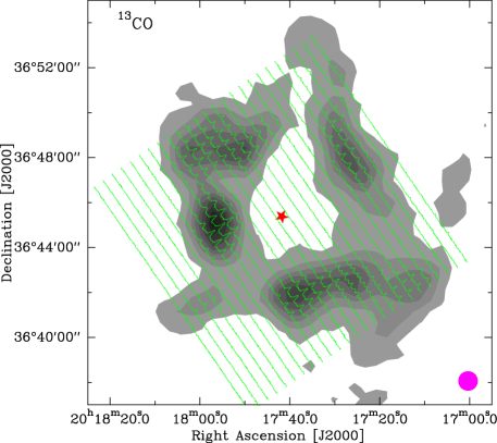
Figure 4: ¹³CO $J$=1-0 spectra overlaid in the integrated intensity image of ¹³CO $J$=1-0 .

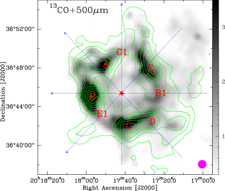
Figure 5: ¹³CO $J$=1-0 integrated intensity map overlaid on the Herschel 500 $\mu$m image (color scale). The green contour levels are from 1.8 (3$\sigma$) to 16.2 by a step of 1.8 K km s^-1. Letters A, B, C, and D indicate the different molecular clumps, while letters A1, B2, C1, and D1 represent the symmetrical position with these clumps in the ring. The red ”star” represent the exciting star. The data used in the position-velocity diagrams (in Figure 6) are selected along the blue arrows. The unit for the colour bar is Jy pixel^-1.

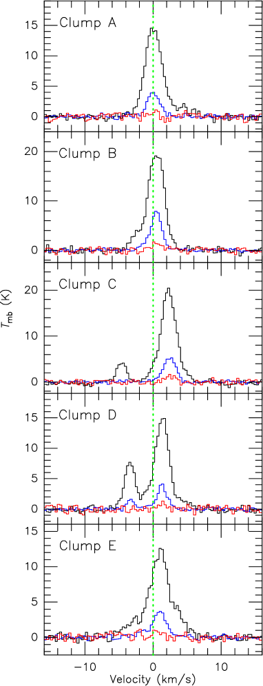
Figure 6: ¹²CO $J$=1-0, ¹³CO $J$=1-0, and C¹⁸O $J$=1-0 spectra at the peak position of the molecular clumps A, B, C, D, and E. The green dashed line indicates the systemic velocity (0 km s^-1) of Sh2-104.

To investigate spatial correlation between gas and dust of the ring around Sh2-104, we made the ¹³CO $J$=1-0 integrated intensity map overlaid on the Herschel 500 $\mu$m emission (Fig. 5). The ¹³CO $J$=1-0 emission in the Fig. 5 is associated with the 500 $\mu$m dust emission in morphology. There are four gas fragments located in the ring. It is different from dust fragments, the southern gas fragment contains two clumps. We designated these clumps at clump A, clump B, clump C, clump D, and clump E. The clump B is more compact relative to other clumps, which is spatially consistent with IRAS 20160+3636. Figure 6 shows the ¹²CO $J$=1-0, ¹³CO $J$=1-0, and C¹⁸O $J$=1-0 spectra toward the peak position of each clump. The line profiles of ¹²CO $J$=1-0 and ¹³CO $J$=1-0 in clump B appear to only show the blue wings, while it displays the blue and red winds in clump E. For clumps C and D, the line profiles of ¹²CO $J$=1-0 and ¹³CO $J$=1-0 show two velocity components. We fitted each spectrum with the Gaussian profile. Table 1 shows the fitted results, including their peak intensities, FWHMs, and central velocities. From Table 1, we can see that the central velocities of these clumps are different. As shown in the Fig. 6, the central velocity of each clump has a shift with respect to the LSR velocity of the ionized gas for Sh2-104, except for the clump A.

3.3 Column Density and Mass of Molecular Ring

To estimate the column density and mass of the molecular ring around Sh2-104, we used the optical thin ¹³CO $J$=1-0 emission. Assuming local thermodynamical equilibrium (LTE), the column density was estimated via Garden et al. (Garden et al., 1991)

$$\mathit{N(\rm^{13}CO)}=4.71\times 10^{13}\frac{T_{\rm ex}+0.88}{\rm exp(-5.29/T_{\rm ex})}\frac{\tau}{\rm 1-exp(-\tau)}W~{}\rm cm^{-2},$$ (1)

where $\tau$ is the optical depth and $T_{\rm ex}$ is the mean excitation temperature of the molecular gas. W is $\int T_{\rm mb}dv$ in units of K km s^-1, $T_{\rm mb}$ is the corrected main-beam temperature of ¹³CO $J$=1-0 and $dv$ is the velocity range.

Table 1: Observed parameters of each line for each clump

Name		12CO J=1-0					13CO J=1-0
	$T_{\rm mb}$	FWHM	$V_{\rm LSR}$			$T_{\rm mb}$	FWHM	$V_{\rm LSR}$
	(K)	(km $\rm s^{-1}$)	(km $\rm s^{-1}$)			(K)	(km $\rm s^{-1}$)	(km $\rm s^{-1}$)
A	14.4	3.1	0.1			4.0	2.0	0.1
B	19.6	2.9	0.5			7.7	2.0	0.6
C	19.5	2.8	2.3			5.3	2.2	2.4
D	14.3	2.7	1.3			3.8	1.8	1.3
E	11.0	4.0	1.0			3.5	2.6	1.0

Generally, the ¹²CO emission is optical thick, so we used ¹²CO to estimate $T_{\rm ex}$ via following the equation (Garden et al., 1991)

$$\mathit{T_{\rm ex}}=\frac{5.53}{{\ln[1+5.53/(T_{\rm mb}+0.82)]}},$$ (2)

where $T_{\rm mb}$ is the corrected main-beam brightness temperature of ¹²CO. From this equation, we derived that the excitation temperature of the five clumps is from 14.4 K to 23.1 K. Since these clumps are regularly located in the ring, then we adopt the mean excitation temperature of about 19.2 K as that of the molecular ring.

Moreover, we assumed that the excitation temperatures of ¹²CO and ¹³CO have the same value in the molecular ring. The optical depth ($\tau$) can be derived using the following equation (Garden et al., 1991)

$$\mathit{\tau(\rm^{13}CO)}=-\ln[1-\frac{T_{\rm mb}}{5.29/[\rm exp(5.29/\it T_{\rm ex})\rm-1]-0.89}],$$ (3)

The obtained optical depth is 0.25-0.67, suggesting that the ¹³CO emission is optically thin in the ring.

In addition, we used the relation $N(\rm H_{2})/\it N(\rm^{13}CO)$ $\approx$ $7\times 10^{5}$ (Castets et al., 1982) to estimate the H₂ column density. The mass of the ring can be determined by

$$\mathit{M_{\rm H_{2}}}=\mu m_{\rm H}\it N(\rm H_{2})\it S,$$ (4)

where $\mu$=2.72 is the mean molecular weight, $m_{\rm H}$ is the mass of a H atom, and $S$ is the projected 2D area of the ring. Hence, we obtained that the mean column density of the ring is 6.8$\times 10^{21}$ cm^-2. Using the mean column density, we derived a mass of $\sim$2.2$\times 10^{4}\rm M_{\odot}$ for the ring.

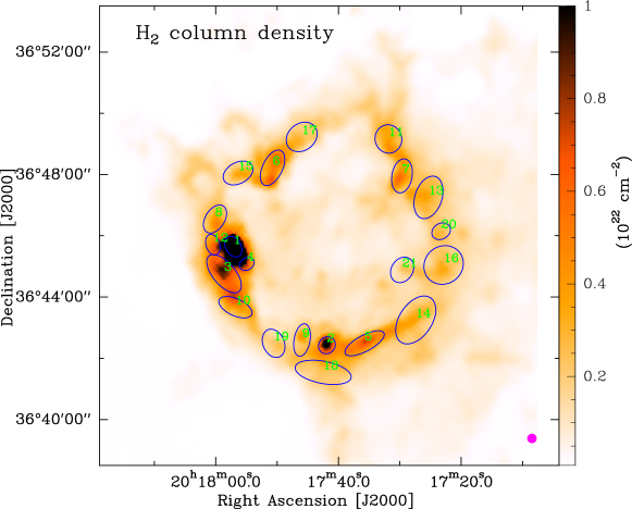
Figure 7: High-resolution (18$\farcs 2$) column density map of the Sh2-104 region derived from Hi-GAL survey data. The blue ellipses indicate the identified clumps.

Table 2: Derived parameters of identified clumps

ID	R.A.	Dec.	$\theta_{\rm min}$	$\theta_{\rm maj}$	$R_{\rm eff}$	$N_{\rm H_{2}}$	Mass	$n_{\rm{}_{H_{2}}}$
	(J2000)	(J2000)	(arcsec)	(arcsec)	(pc)	(1022 cm-2)	(M⊙)	(cm-3)
1	20:17:54.7	36:45:38.5	30.0	43.7	0.30	2.8	251.1	5225
2	20:17:42.5	36:42:25.5	31.8	34.9	0.27	1.1	82.6	1912.2
3	20:17:55.9	36:44:45.7	43.7	91.3	0.58	1.0	330.0	1097.1
4	20:17:53.0	36:45:04.9	24.1	30.5	0.19	0.8	29.8	2317.7
5	20:17:37.6	36:42:29.3	31.6	85.9	0.45	0.7	151.4	1270.6
6	20:17:49.6	36:48:13.2	39.1	75.0	0.49	0.7	156.8	843.6
7	20:17:32.7	36:47:57.3	39.8	67.5	0.46	0.6	127.4	737.6
8	20:17:57.1	36:46:32.8	37.9	60.6	0.42	0.5	89.9	664.2
9	20:17:45.7	36:42:35.7	31.6	64.6	0.39	0.4	67.3	766.9
10	20:17:54.4	36:43:40.1	52.2	55.9	0.49	0.5	111.2	413.4
11	20:17:34.5	36:49:09.7	27.0	42.1	0.27	0.6	42.8	1328.1
12	20:17:57.4	36:45:42.4	52.9	86.2	0.63	0.4	155.9	353.1
13	20:17:29.2	36:47:15.2	64.2	104.6	0.77	0.4	218.1	263.1
14	20:17:30.9	36:43:15.0	73.5	79.8	0.72	0.3	169.3	202
15	20:17:54.1	36:48:03.0	52.5	65.4	0.54	0.3	88.7	273.9
16	20:17:27.3	36:45:02.7	41.6	57.8	0.44	0.3	51.1	312.3
17	20:17:45.8	36:49:13.5	42.0	53.1	0.42	0.2	41.5	273.4
18	20:17:43.0	36:41:32.4	33.4	70.1	0.42	0.5	83.5	738.3
19	20:17:49.5	36:42:29.3	41.5	62.2	0.46	0.4	78.5	446.3
20	20:17:27.6	36:46: 8.9	43.7	111.7	0.64	0.3	121.3	328.5
21	20:17:32.7	36:44:53.1	30.6	38.7	0.28	0.2	19.2	439.3

Table 3: Properties of identified clumps around the H II region Sh2-104

ID	$T_{\rm mb}$(12)	FWHM(12)	$V_{\rm LSR}$(12)	$T_{\rm mb}$(13)	FWHM(13)	$V_{\rm LSR}$(13)	$T_{\rm ex}$	$\sigma_{\rm{}_{Therm}}$	$\sigma_{\rm{}_{NT}}$	$\sigma_{\rm{}_{v}}$	$\alpha$
	(K)	(km s-1)	(km s-1)	(K)	(km s-1)	(km s-1)	(K)	(cm-3)
1	13.5(0.5)	3.9(0.1)	0.1(0.1)	5.4(0.2)	2.6(0.1)	-0.2(0.1)	17.0(0.5)	0.22(0.01)	1.10(0.02)	1.12(0.01)	1.8
2	12.0(1.2)	3.5(0.2)	2.5(0.1)	4.2(0.3)	2.2(0.1)	2.5(0.1)	15.4(0.5)	0.21(0.01)	0.92(0.03)	0.94(0.02)	3.5
3	16.1(0.5)	3.0(0.1)	0.6(0.1)	6.1(0.2)	1.9(0.1)	0.6(0.1)	19.6(0.5)	0.24(0.01)	0.79(0.02)	0.83(0.01)	1.5
4	17.2(0.5)	3.3(0.1)	0.4(0.1)	6.3(0.2)	2.2(0.1)	0.2(0.1)	20.7(0.5)	0.25(0.01)	0.94(0.02)	0.97(0.01)	7.2
5	15.2(1.7)	2.4(0.1)	1.7(0.1)	4.6(0.3)	1.8(0.1)	1.7(0.1)	18.7(0.5)	0.23(0.11)	0.77(0.02)	0.80(0.01)	2.3
6	15.2(1.2)	3.3(0.1)	0.6(0.1)	4.2(0.3)	2.6(0.1)	0.5(0.1)	18.7(0.5)	0.23(0.01)	1.09(0.03)	1.12(0.02)	4.7
7	5.3(0.5)	6.2(0.2)	0.3(0.1)	2.1(0.3)	2.4(0.2)	0.6(0.1)	8.6(0.5)	0.16(0.01)	1.02(0.08)	1.03(0.04)	4.6
8	9.7(0.5)	4.0(0.1)	0.1(0.1)	2.0(0.3)	3.5(0.2)	-0.1(0.1)	13.1(0.5)	0.20(0.01)	1.47(0.07)	1.48(0.04)	12.3
9	–	–	–	–	–	–	–	–	–	–	–
10	9.1(0.8)	2.8(0.2)	1.0(0.1)	3.8(0.3)	1.4(0.1)	1.1(0.1)	12.5(0.8)	0.19(0.01)	0.59(0.03)	0.62(0.01)	2.0
11	9.9(0.5)	3.1(0.1)	1.0(0.1)	2.4(0.3)	2.1(0.1)	0.8(0.1)	13.3(0.5)	0.20(0.01)	0.90(0.05)	0.92(0.02)	6.4
12	8.5(0.5)	4.4(0.1)	-0.4(0.1)	2.8(0.3)	3.2(0.1)	-0.4(0.1)	11.8(0.5)	0.19(0.01)	1.38(0.05)	1.40(0.02)	9.5
13	8.9(0.6)	5.2(0.1)	1.2(0.1)	2.3(0.3)	2.4(0.2)	1.7(0.1)	12.3(0.6)	0.19(0.01)	1.02(0.09)	1.04(0.04)	4.6
14	8.2(0.5)	6.5(0.1)	0.3(0.1)	2.3(0.6)	1.7(0.2)	1.3(0.1)	11.6(0.5)	0.18(0.01)	0.74(0.08)	0.76(0.04)	2.9
15	15.6(0.5)	3.0(0.1)	0.4(0.1)	4.3(0.3)	2.2(0.1)	0.3(0.1)	19.1(0.5)	0.24(0.01)	0.92(0.02)	0.95(0.01)	6.6
16	3.6(0.5)	9.7(0.1)	0.7(0.1)	0.9(0.3)	3.0(0.5)	3.7(0.2)	6.8(0.5)	0.14(0.01)	1.27(0.20)	1.28(0.10)	16.9
17	8.9(0.6)	3.3(0.2)	0.1(0.1)	2.6(0.3)	2.2(0.1)	-0.2(0.1)	12.3(0.6)	0.19(0.01)	0.91(0.05)	0.93(0.02)	10.5
18	16.8(1.2)	2.7(0.1)	2.4(0.1)	4.1(0.3)	2.0(0.1)	2.6(0.1)	20.3(0.5)	0.24(0.01)	0.82(0.03)	0.86(0.01)	4.5
19	6.0(0.5)	2.8(0.1)	0.7(0.1)	0.7(0.3)	3.4(0.4)	0.5(0.2)	9.3(0.5)	0.17(0.01)	1.43(0.18)	1.44(0.09)	14.6
20	4.1(0.5)	7.3(0.2)	-0.7(0.1)	1.2(0.3)	2.2(0.3)	-2.2(0.1)	7.4(0.5)	0.15(0.01)	0.92(0.13)	0.93(0.07)	5.5
21	–	–	–	–	–	–	–	–	–	–	–

3.4 Clumps Extraction

Clumps with star formation activities are always found on the border of H II region. The Hi-GAL survey data can be used to construct column density (N${}_{H_{2}}$) map of the studied region. From the column density map, we can extract clumps. Previous method that the obtained column density maps is at the 36$\farcs 3$ resolution of SPIRE 500 $\mu$m. To reveal more small structures, Palmeirim et al. (2013) construct a column density map at the 18$\farcs 2$ resolution of the SPIRE 250 $\mu$m data for the B211+L1495 region. Within the region covered by both PACS and SPIRE, the reliability of the smoothed 250 $\mu$m version agrees with that at the smoothed 500 $\mu$m. Based on the smoothed 250 $\mu$m method of Palmeirim et al. (2013), the column density map of Sh2-104 were created using a modified blackbody model to fit the SEDs pixel by pixel. In Hi-GAL five bands, we only use 160, 250, 350 and 500 $\mu$m. Emission at 70 μm was excluded in the SED fitting because it can be contaminated by emission from small grains in hot PDRs. The dust opacity law is assumed as $\kappa_{\upsilon}$ = 0.1$\times$(300 $\mu m/\lambda$)^β cm²/g, with $\beta$=2. The corresponding column density map of Sh2-104 is given in Fig. 7, which shows a ring-like structure. The column density of the ring ranges from $\sim 10^{21}$ cm^-2 to $\sim 10^{22}$ cm^-2. Using ¹³CO $J$=1-0 molecular line, the obtained mean column density of the ring is 6.8$\times 10^{21}$ cm^-2, which is in agreement with that from Hi-GAL data.

We use the algorithms Gaussclumps (Stutzki & Guesten, 1990; Kramer et al., 1998; Zhang et al., 2017) to extract clumps and derive their physical properties from the column density map. Gaussclumps is a task included in the GILDAS package. Although Gaussclumps was originally written to decompose a three-dimensional data cube into Gaussian-shaped sources, it can also be applied to dust continuum or column density maps without modification of the code. Kramer et al. (1998) suggested that “Stiffness” parameters that control the fitting were set to 1. A peak flux density threshold was set to 5$\sigma$. According to Belloche et al. (2011), the initial guesses for the aperture cutoff, the aperture FWHM and the source FWHM were adopted as 8, 3, and 1.5 times the angular resolution, respectively. In Table 2, we display all the clumps identified with Gaussclumps. Columns are (1) identification number of the clumps, (2)–(3) J2000 positions, (4)–(5) the major and minor deconvolved FWHM of the clumps, (7) H₂ column density.

3.5 Size, Mass and Volume Density

Using the major and minor deconvolved FWHM ($\theta_{\rm maj}$ and $\theta_{\rm min}$) of the clumps, the effective deconvolved radius of these clumps was determined by

$$\mathit{R_{\rm eff}}=\sqrt{\theta_{\rm min}\times\theta_{\rm maj}}/2,$$ (5)

The obtained $R_{\rm eff}$ are listed in column 6 of Table 2. Clump radius are found to lie between 0.19 pc and 0.77 pc.

In addition, the total mass of the clumps was calculated from their H₂ column density (Kauffmann et al., 2008),

$$\mathit{M}=\mu m_{\rm H}\int N_{\rm H_{2}}\rm d\it A,$$ (6)

Where $\mu$=2.72 is the mean molecular weight, $m_{\rm H}$ is the mass of an H atom, and the surface element $\rm d\it A$ is ralated to the solid angle d$\Omega$ by $\rm d\it A$=$D^{2}$d$\Omega$, where $D$ is the distance of the clumps.

Assuming a 3D geometry for the clumps, the average volume density of each clump was calculated as

$$\mathit{n_{\rm H_{2}}}=\frac{M}{4/3\pi R_{\rm min}^{2}R_{\rm maj}\mu m_{\rm H}},$$ (7)

Where $R_{\rm min}$ and $R_{\rm maj}$ are the respective minor and major axes of the clumps. The obtained volume densities are listed in Table 2.

3.6 Velocity Dispersion and Virial Parameter($\alpha$)

From H₂ column density map, 21 clumps are identified. Based on their coordinates and size, we search for ¹²CO $J$=1-0 and ¹³CO $J$=1-0 spectra that are located at or near the peak position of the clumps. Morever, we fitted the spectrum of each clump with the Gaussian profile. The fitted parameters are listed in Table 3, including brightness temperature ($T_{\rm mb}$), FWHM, and centroid velocity ($V_{\rm LSR}$). For clumps 9 and 21, we did not obtain the effective spectral value because of the weak signal ($\leq 3\sigma$). Since the ¹³CO $J$=1-0 emission is optically thin in the ring (see Sec. 3.3), we use the FWHM of ¹³CO $J$=1-0 to calculate the one-dimensional velocity dispersion ($\sigma_{\upsilon}$). Because these clumps are distributed mainly over the molecular ring associated with Sh2-104, we also need consider the thermal velocity dispersion. $\sigma_{\upsilon}$ in each clump is calculated as follows:

$$\mathit{\sigma_{\upsilon}}=\sqrt{\sigma_{\rm Therm}^{2}+\sigma_{\rm NT}^{2}}$$ (8)

Where $\sigma_{\rm Therm}$ and $\sigma_{\rm NT}$ are the thernal and non-thermal one-dimensional velocity dispersions. For all the clumps, $\sigma_{\rm Therm}$ and $\sigma_{\rm NT}$ can be derived as, respectively:

$$\mathit{\sigma_{\rm Therm}}=\sqrt{\frac{kT_{\rm ex}}{m_{\rm H}\mu}}$$ (9)

$$\mathit{\sigma_{\rm NT}}=[\sigma_{\rm{}^{13}CO}^{2}-\frac{kT_{\rm ex}}{m_{\rm{}^{13}CO}\mu}]^{1/2}$$ (10)

Where $T_{\rm ex}$ is the excitation temperature of the clumps. We used ¹²CO $J$=1-0 to calculate $T_{\rm ex}$ following equation 2. $\sigma_{\rm{}^{13}CO}$ = ($\Delta V_{13}/\sqrt{\rm 8ln2}$) is the one-dimensional velocity dispersion of ¹³CO $J$=1-0 while $m_{\rm{}^{13}CO}$ is the mass of ¹³CO $J$=1-0. The derived parameters are summaried in Table 3.

Stability of the clumps against gravitational collapse can be evaluated using the virial parameter (Kauffmann et al., 2013)

$$\mathit{\alpha}=1.2(\frac{\sigma_{\upsilon}}{\rm km\ s^{-1}})^{2}(\frac{R_{\rm eff}}{\rm pc})(\frac{M}{10^{3}M_{\odot}})^{-1}$$ (11)

Where $\sigma_{\upsilon}$ is the one-dimensional velocity dispersion, $R_{\rm eff}$ is the effective deconvolved radius, and $M$ is the mass of the clumps. If $\alpha\leq 2$, the clumps collapse (Bertoldi & McKee, 1992; Kauffmann et al., 2013). Hence, from Table 3, we obtain that clumps 1, 3, and 10 collapse.

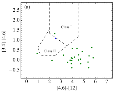
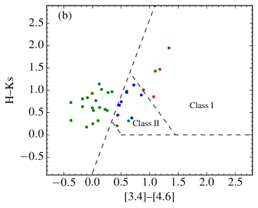
Figure 8: Left panel: WISE bands 1, 2, 3 color-color diagram. Right panel: WISE bands 1 and 2 and 2MASS H and Ks color–color diagram. Dashed lines indicate the boundaries by which we classify Class I and Class II. Class I YSOs are labelled as red dots, and class II YSOs as blue dots. The green dots indicate Class I/II YSOs from (Marton et al., 2016).

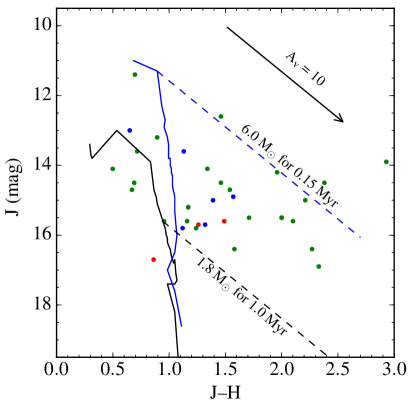
Figure 9: J/J-H colour-magnitude diagram for the YSOs. Class II YSOs are labelled as red dots, and Class I YSOs as blue dots. The green dots indicate Class I/II YSOs from (Marton et al., 2016). The black solid curve denotes the location of 10⁶ yr old pre–main-sequence (PMS) stars, and the blue solid curve is for those that is 1.5$\times$10⁶ yr old, both were obtained from the model of Siess et al. (2000). All the isochrones are corrected for the distance and reddening of the Sh2-104 region. Dashed lines represent reddening vectors for various masses. The black dashed line denotes the position of a PMS star of 1.8 M_⊙ for 1.0 Myr, and the blue dashed lines indicate the position of star of 6.0 M_⊙ for 0.15 Myr.

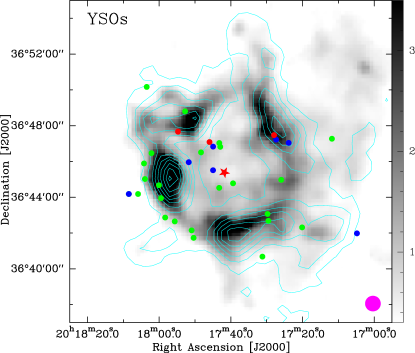
Figure 10: ¹³CO $J$=1-0 integrated intensity map overlaid on the Hersel 500 $\mu$m image (grey scale). Class II YSOs are labelled as red dots, and Class I YSOs as blue dots. The green dots indicate Class I/II YSOs from (Marton et al., 2016). The unit for the colour bar is Jy pixel^-1.

3.7 Distribution of Young Stellar Objects

To detect young stellar objects (YSOs) adjacent to Sh2-104, we use the WISE and 2MASS all-sky source catalogs (Skrutskie et al., 2006; Wright et al., 2010). From these two catalogs, we select the sources with the 3.4, 4.6, 12, and 22 $\mu$m, and $J$, $H$, and $Ks$ bands within a circle of 9^′ in radius centered on the ionized star of Sh2-104. We select YSOs using the criteria described in Koenig & Leisawitz (2014), as shown in Fig. 8. This criteria is based on the $[4.6]-[12.0]$ versus $[3.4]-[4.6]$ color-color, and $[Ks]-[3.4]$ versus $[3.4]-[4.6]$ color-color diagrams. For many objects visible in WISE bands 1 and 2 will lack a reliable band 3 or 4 detection, the $[3.4]-[4.6]$ versus $[H]-[Ks]$ color-color diagram is a supplement to $[4.6]-[12.0]$ versus $[3.4]-[4.6]$ color-color diagram. Based on above color selection criteria of YSOs, we only find 3 Class I YSOs and 8 Class II YSOs. Furthermore, a much cleaner selection technique has been used by Marton et al. (2016) to create an all-sky catalogue of YSOs (Class I/II). According to the catalogue of Marton et al. (2016), we find 23 Class I/II YSOs. Comparing the YSO positions, only an YSO overlap between the two methods. Class I YSOs are protostars with circumstellar envelopes, while Class II YSOs are disk-dominated objects (Evans et al., 2009). The $J$ luminosity is used to estimate stellar masses, as $J$ is less affected by the emission from circumstellar material (Bertout et al., 1988; Yadav et al., 2016). Figure 9 shows the $J/J-H$ colour-magnitude diagram for the selected YSOs. The black solid curve denotes the location of 10⁶ yr old pre-main-sequence (PMS) stars, and the blue solid curve is for those that is 1.5$\times$10⁶ yr old, both were obtained from the model of Siess et al. (2000). All the isochrones are corrected for the distance and reddening of the Sh2-104 region. Dashed lines represent reddening vectors for various masses. The black dashed line denotes the position of a PMS star of 1.8 M_⊙ for 1.0 Myr, and the blue dashed lines indicate the position of star of 6.0 M_⊙ for 0.15 Myr. From Fig. 9, we see that the majority of the YSOs have masses in the range 1.8-6.0 M_⊙, and an age range of 0.15-1.0 Myr. Figure 10 shows the spatial distribution of both Class I and Class II YSOs. From Fig. 10, we also note that Class I/II YSOs are mostly concentrated along the molecular and dust ring.

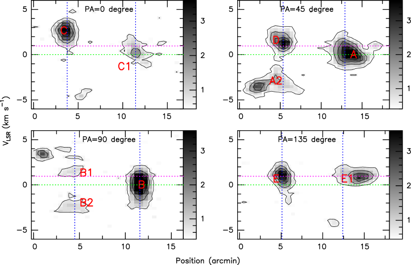
Figure 11: P-V diagrams constructed from ¹³CO $J=1-0$ transition for different directions. The contour levels are 10, 20,…, $90\%$ of the peak value. The blue dashed lines show the projected position of each edge in the different position angle, while the green dashed lines indicate the systemic velocity (0 km s^-1) of Sh2-104; The pink dashed lines indicate the systemic velocity of 1 km s^-1.

4 Discussion

4.1 Gas Structure Around Sh2-104

The ionized gas of Sh2-104 shows a ring-like structure with a radius of about 2.9 pc (2.5^′at 4 kpc), which is consistent with the optical image (Deharveng et al., 2003). Deharveng et al. (2010) studied 102 bubbles. Only bubbles N49 and N61 show a shell-like structure in both the radio continuum emission and the 24 $\mu$m emission (Watson et al., 2008; Xu et al., 2016). They suggested that such shell-like structure could be due to a stellar wind emitted by the central massive star. Both CO molecular gas and cool dust emission shows a ring-like shape, which just encloses the ionized gas of Sh2-104. If an H II region spherically expands, both the collected gas and dust emission will also show three-dimensional spherical shell structure. However, Beaumont & Williams (2010) suggested that the collected gas and dust emission around H II region is two-dimensional rings with thicknesses not greater than the ring sizes. For the three-dimensional shells, expanding along the line of sight will result in blue-shifted emission from the near-side of the shell, and red-shifted emission from the far side (Anderson et al., 2015). Here for the CO molecular ring surrounded H II region Sh2-104, we also did not detect the CO emission of higher than 3 signal (0.6 K) inside the ring.

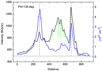
Figure 12: Slice profiles of WISE 12 $\mu$m emission (black lines) and H₂ column density map (blue lines) through Sh2-104 in PA = 45degree and PA = 135 degree directions. The cutting paths are shown as the green arrows in Fig. 11. The red dashed lines mark the two edges of Sh2-104, while the green lines may indicate some gas emission.

To further reveal the structure of the ring, we made four position-velocity (PV) diagrams in ¹³CO $J$=1-0 line, as shown in Fig. 11. These PV diagrams are obtained from the four cuts through the position of the exciting star with the position angles (PA) of 0^∘, 45^∘, 90^∘, and 135^∘ (see Fig. 5). From Fig. 11, we see that the symmetrical borders of the ring are detected along all the four cuts. Each border is marked by a blue dashed line. Between two symmetrical borders, we still did not detect the CO emission. Since our selected cuts just go through these identified clumps, then the position of each clump can indicate a border of the ring. For the symmetrical borders, we design name at clumps A1, B1, C1, D1, and E1. If one border has two CO components, the other component will be named such as clumps A2 and B2. Through inspected the clumps A2 and B2 with association of the Sh2-104 morphology, we suggest that there two clumps should belong to the foreground emission of the corresponding border, and only overlap with the other component in the line of sight. Through the PV diagrams (Fig. 11), we found that both the borders of the ring with clumps E and E1 have a systemic velocity of about 1 ${\rm km~{}s}^{-1}$. The cut line through clumps E and E1 divide the ring into the north-east and south-west two portions. The north-east portion containing the clumps A, B, and C1 is blueshifted, while the south-west portion with the clumps B1, C, and D is redshifted. Hence, we concluded that the ring is expanding with an inclination relative to the plane of sky. The existence of the inclination indicates that the ring is not spherically symmetrical. Additionally, from Fig. 11, we also see that the projected distances are the same and 7.5^′ between two symmetrical edges along the different PAs. The distance between clumps E and E1 is roughly equal to their projected distance. While the distances between clumps C and C1, clumps A and D, clumps B and B1 are greater than 7.5^′, because the cut lines through two symmetrical clumps have an inclination angle with the projected axis. It further suggests that the ring is not spherically symmetrical. The ionized gas of Sh2-104 has a LSR velocity of about 0 ${\rm km~{}s}^{-1}$ (Georgelin et al., 1973). While the expansion of the molecular ring begin at the LSR velocity of 1 ${\rm km~{}s}^{-1}$. If there is a three-dimensional spherical shell that just encloses Sh2-104, the ionized gas and the ring should have the same LSR velocity. From above analysis, we concluded that the collected gas emission around H II region Sh2-104 may be a two-dimensional ring-like structure.

In addition, we also make the slice profiles of WISE 12 $\mu$m emission (black lines) and H₂ column density map (blue lines) through Sh2-104 in PA = 45 degree and PA = 135 degree directions, as shown in Fig. 12, which shows the 12 $\mu$m flux and H₂ column density change as a function of the position. The two symmetrical borders (red dashed lines) of the ring related to Sh2-104 display the strang 12 $\mu$m and H₂ emission, indicating that the strang PAHs molecules traced by the 12 $\mu$m emission are excited only if there should be some molecular gas adjacent to H II region. Howerver, the 12 $\mu$m emission is very strang inside the ring, while the H₂ column density is lower in the corresponding positions. Compared with the 70 $\mu$m emission in the left panel of Fig. 2, we that found the 12 $\mu$m emission is associated with that at 70 $\mu$m inside the ring, suggesting that this part of the 12 $\mu$m emission is also producted from the hot dust. Thus, it further confirms that the collected gas emission is likely to a two-dimensional ring-like structure around H II region Sh2-104.

4.2 Star Formation Scenario

Five large clumps are regularly spaced along the ring. One of these clumps is associated with an UCHII region and IRAS 20160+3636. Deharveng et al. (2003) suggested that the CC process is at work in this region. From the high-resolution (18$\farcs 2$) column density map constructed by the Hi-GAL survey data, we extract 21 clumps. To determine whether the identified clumps have sufficient mass to form massive stars, we must consider their sizes and mass. According to Kauffmann & Pillai (2010), if the clump mass is $M(r)\geq 580M_{\odot}(r/\rm pc)^{1.33}$, thus they can potentially form massive stars. Figure 13 presents a mass versus radius plot of the clumps. We find that only two clumps (#1 and #3) above the threshold, indicating that these two clumps are dense and massive enough to potentially form massive stars. About 90% of all the identified clumps will form low-mass stars. Moreover, we evaluate the stability of these clumps against gravitational collapse using the virial parameter, finding only three clumps collapse, including clumps #1 and #3. The surface density of 0.024 g cm^-2 gives the average surface density thresholds for efficient star formation. The thresholds, shown in green lines in Fig. 13, are derived by (Lada et al., 2010; Heiderman et al., 2010), respectively. As can be seen from Fig. 13, 15 clumps (72%) lie at or above the lower surface density limit of 0.024 g cm^-2. A power-law fit to the identified clumps yields $M(r)=281M_{\odot}(r/\rm pc)^{1.31\pm 0.08}$. The slope we obtained is equal to what was found in Kauffmann & Pillai (2010).

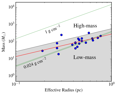
Figure 13: Mass versus radius relationship. The grey region represents the parameter space to be devoid of massive star formation. The black line delineates the threshold (Kauffmann & Pillai 2010). The blue solid circles indicate the clumps. Upper and lower solid green lines present surface densities of 1 g cm^-2 and 0.024 g cm^-2, respectively. The red line shows the result of a power-law fit to all the clumps, where we find $M(r)=281M_{\odot}(r/\rm pc)^{1.31\pm 0.08}$.

The selected YSOs (Class I and Class II ) are mostly concentrated in the whole ring around H II region Sh2-104. The high density of YSOs located in the ring that these YSOs are physically associated with Sh2-104. The dynamical age of Sh2-104 can be used to decide whether these YSOs are triggered by the H II region. Using a simple model described by (Dyson & Williams, 1980) and assuming an H II region expanding in a homogeneous medium, we estimate the dynamical age of the H II region as

$$\mathit{t_{\rm dyn}}=\frac{4R_{\rm s}}{7c_{\rm s}}[(\frac{R}{R_{\rm s}})^{7/4}-1],$$ (12)

where $R_{\rm s}$ is the radius of the Strömgren sphere given by $R_{\rm s}$ = $3Q_{\rm Ly}/4\pi n_{0}^{2}\alpha_{\rm B}$, where $Q_{\rm Ly}$ is the ionizing luminosity, $n_{\rm 0}$ is the initial number density of the ambient medium around the H II region, $\alpha_{\rm B}$ = 2.6$\times$10^-13 cm³ s^-1 is the hydrogen recombination coefficient to all levels above the ground level. For the ionized medium we adopt a sound velocity of $c_{\rm s}$ $\simeq$ 10 km s^-1. Moreover, we adopt the radius (3.7^′) of the ring as that of H II region Sh2-104, which is obtained from Fig. 11. Taking the distance of $\sim$4 kpc to Sh2-104 (Deharveng et al., 2003), the H II region radius is 4.4 pc. As a rough estimate, $n_{\rm 0}$ can be determined by distributing the total molecular mass over a sphere (e.g., Zavagno et al., 2007; Paron et al., 2009; Cichowolski et al., 2009; Anderson et al., 2015; Duronea et al., 2015). The mass of the ring is $\sim$2.2$\times 10^{4}\rm M_{\odot}$. Using this mass, we only consider the number of atoms that can be ionized, so this would imply that $n_{\rm 0}$ = 2.6$\times 10^{3}$ cm^-3. H II region Sh2-104 is excited by an O6V center star (Crampton et al., 1978; Lahulla, 1985). For an O6V star, the ionizing luminosity ($Q_{\rm Ly}$) is 10^48.99 $\rm s^{-1}$ (Martins et al., 2005). Inoue (2001) suggested that only half of Lyman continuum photons from the central source in a Galactic H II region ionizes neutral hydrogen, the remainder being absorbed by dust grains within the ionized region. Finally, we obtain the ionizing luminosity of 10^48.69 $\rm s^{-1}$. Hence, we derived a dynamical age of 1.6$\times 10^{6}$ yr for H II region Sh2-104. Additionaly, from the $J/J-H$ colour-magnitude diagram for the selected YSOs, we derive that the majority of the YSOs have masses in the range 1.8-6.0 M_⊙, and an age range of 0.15-1.0 Myr. Comparing the dynamical age of H II region Sh2-104 with that of YSOs shown on the ring, we conclude that these YSOs are likely to be triggered by H II region Sh2-104. It also means that the CC or RDI processes induce the formation of these YSOs. Deharveng et al. (2003) suggested H II region Sh2-104 is a typical candidate for triggering star formation by CC process.

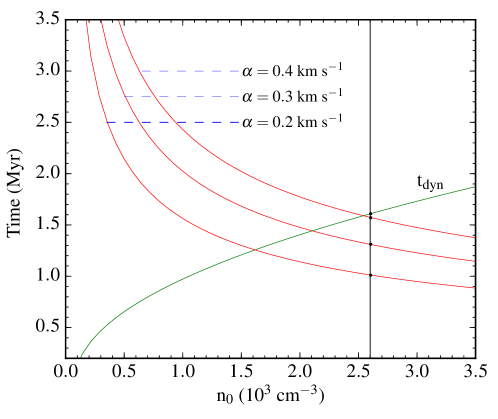
Figure 14: plot of dynamical time (green curve) and fragmentation timescale (red curves) as a function of initial density of the ambient medium. The fragmentation timescale is calculated for different sound speeds of neutral gas ($\alpha_{s}$ = 0.2, 0.3, and 0.4 km s^-1). The black vertical line marks the position of n₀ = 2.6$\times 10^{3}$ cm^-3.

The expansion of Sh2-104 have collected the gas into the ring. To determine whether the fragmentation occurs around Sh2-104 via the CC process, we compute the fragmentation time of the collected gas based on the theoretical model of Whitworth et al. (1994) :

$$\mathit{t_{\rm frag}}=1.56(\frac{\alpha_{\rm s}}{0.2})^{7/11}(\frac{Q_{\rm Ly}}{10^{49}})^{-1/11}(\frac{n_{0}}{10^{3}})^{-5/11}\rm\ Myr,$$ (13)

The diagram of $t_{\rm frag}$ and $t_{\rm dyn}$ as a function of the initial ambient density $n_{0}$ is shown in Fig. 14. In comparison, we find that the dynamical age of H II region Sh2-104 ($t_{\rm dyn}$ $\approx$ 1.6 Myr) is greater than the fragmentation time. This indicates that the ring of the collected gas has had enough time to fragment into the identified clumps during the lifetime of H II region Sh2-104. Thus, it further confirm that the CC process is presumably at work H II region Sh2-104.

5 CONCLUSIONS

We present the molecular ¹²CO $J$=1-0, ¹³CO $J$=1-0 and C¹⁸O $J$=1-0, infrared, and radio continuum observations toward H II region Sh2-104. The main results are summarized as follows:

1. H II region Sh2-104 shows a double-ring structure, the outer ring traced by 12 $\mu$m, 500 $\mu$m, ¹²CO $J$=1-0, and ¹³CO $J$=1-0 emission, and the inner ring traced by by 22 $\mu$m and 21 cm emission. We suggest that the outer ring with a radius of 4.4 pc is created by the expansion of H II region Sh2-104, while the inner ring with a radius of 2.9 pc may be produced by the energetic stellar wind from its central ionized star. We derived a dynamical age of 1.6$\times 10^{6}$ yr for H II region Sh2-104.

2. Five large clumps are found to be regularly distributed along the molecular ring. One of these clumps is associated with an UCHII region and IRAS 20160+3636. The column density and mass of the molecular ring is 6.8$\times 10^{21}$ cm^-2 and $\sim$2.2$\times 10^{4}\rm M_{\odot}$. For the CO molecular ring surrounded H II region Sh2-104, we also did not detect the CO emission of higher than 3 signal inside the ring. The north-east portion of the ring is blueshifted relative to the LSR velocity of 1 ${\rm km~{}s}^{-1}$, while the south-west portion is redshifted. Hence, the ring is expanding. We concluded that the collected gas emission around H II region Sh2-104 may be a two-dimensional ring-like structure.

3. From the high-resolution (18$\farcs 2$) column density map constructed by the Hi-GAL survey data, we extract 21 clumps. The mass-radius relationship for the clumps shows that about 90% of all the identified clumps will form low-mass stars. Moreover, we evaluate the stability of these clumps against gravitational collapse using the virial parameter, finding only three clumps collapse. A power-law fit to the identified clumps yields $M=281M_{\odot}(r/\rm pc)^{1.31\pm 0.08}$. The slope is similar to what was found in Kauffmann & Pillai (2010).

4. The selected YSOs are distributed along the ring around H II region Sh2-104. Comparing the dynamical age of H II region Sh2-104 with the YSOs timescale and the fragmentation time of the molecular ring, we further conclude that these YSOs may be triggered by H II region Sh2-104, and the CC process is at work in this region.

References

- Anderson et al. (2012) Anderson, L. D., Zavagno, A., Deharveng, L., et al. 2012, A&A, 542, A10
- Anderson et al. (2015) Anderson, L. D., Deharveng, L., Zavagno, A., et al. 2015, ApJ, 800, 101
- Anderson et al. (2014) Anderson, L. D., Bania, T. M., Dana, D. S., et al. 2014, ApJS, 212, 1
- Beaumont & Williams (2010) Beaumont, C. N., & Williams, J. P. 2010, ApJ, 709, 791
- Belloche et al. (2011) Belloche, A., Schuller, F., Parise, B., et al. 2011, A&A, 527, A145
- Bertoldi & McKee (1992) Bertoldi, F., & McKee, C. F. 1992, ApJ, 395, 140
- Bertout et al. (1988) Bertout, C., Basri G., & Bouvier, J., 1988, ApJ, 330, 350
- Brand et al. (2011) Brand, J., Massi, F., Zavagno, A., Deharveng, L., & Lefloch, B. 2011, A&A, 527, 62
- Castets et al. (1982) Castets, A., Langer, W. D., & Wilson, R. W. 1982, ApJ, 262, 590
- Cichowolski et al. (2009) Cichowolski, S., Romero, G. A., Ortega, M. E., Cappa, C. E., & Vasquez, J. 2009, MNRAS, 394, 900
- Condon et al. (1998) Condon, J. J., Cotton, W. D., Greisen, E. W., et al. 1998, AJ, 115, 1693
- Crampton et al. (1978) Crampton, D., Georgelin, Y. M., & Georgelin, Y. P. 1978, A&A, 66, 1
- Dyson & Williams (1980) Dyson, J. E., & Williams, D. A. 1980, Physics of the interstellar medium, ed. Dyson, J. E. & Williams, D. A.
- Deharveng et al. (2003) Deharveng, L., Lefloch, B., Zavagno, A., et al. 2003, A&A, 408, 25
- Deharveng et al. (2005) Deharveng, L., Zavagno, A., & Caplan, J. 2005, A&A, 433, 565
- Deharveng et al. (2008) Deharveng, L., Lefloch, B., Kurtz, S., et al. 2008, A&A, 482, 585
- Deharveng et al. (2010) Deharveng, L., Schuller, F., Anderson, L. D., et al. 2010, A&A, 523, A6
- Deharveng et al. (2015) Deharveng, L., Zavagno, A., & Samal, M. R. 2015, A&A, 582, A1
- Duronea et al. (2015) Duronea, N. U., Vasquez, J., Gómez, L., et al. 2015, A&A, 682, A2
- Elmegreen & Lada (1977) Elmegreen, B. G. & Lada, C. J. 1977, ApJ, 214, 725
- Evans et al. (2009) Evans, N. J., II, Dunham, M. M., Jørgensen, J. K., et al. 2009, ApJS, 181, 321
- Faimali et al. (2012) Faimali, A., Thompson, M. A., Hindson, L., et al. 2012, MNRAS, 426, 402
- Garden et al. (1991) Garden, R. P., Hayashi, M., Hasegawa, T., et al., 1991, ApJ, 374, 540
- Georgelin et al. (1973) Georgelin, Y. M., Georgelin, Y. P., & Roux, S. 1973, A&A, 25, 337
- Griffin et al. (2010) Griffin, M. J., Abergel, A., Abreu, A., et al. 2010, A&A, 518, L13
- Heiderman et al. (2010) Heiderman, A., Evans, II, N. J., Allen, L. E., Huard, T., & Heyer, M. 2010, ApJ, 723, 1019
- Inoue (2001) Inoue, A. K. 2001, AJ, 122, 1788
- Kramer et al. (1998) Kramer, C., Stutzki, J., Rohrig, R., & Corneliussen, U. 1998, A&A, 329, 249
- Kauffmann et al. (2008) Kauffmann, J., Bertoldi, F., Bourke, T. L., Evans, N. J., II., & Lee, C. W. 2008, A&A, 487, 993
- Kauffmann et al. (2013) Kauffmann, J., Pillai, T., & Zhang, Q. 2013, ApJ, 765, L35
- Kauffmann & Pillai (2010) Kauffmann, J., & Pillai, T. 2010, ApJ, 723, L7
- Kendrew et al. (2012) Kendrew, S., Simpson, R., Bressert, E., et al. 2012, ApJ, 755, 71
- Kendrew et al. (2016) Kendrew, S., Beuther, H., Simpson, R., et al. 2016, ApJ, 825, 142
- Koenig & Leisawitz (2014) Koenig, X. P., & Leisawitz, D. T. 2014, ApJ, 791, 131
- Kutner & Ulich (1981) Kutner, M. L.,& Ulich, B. L. 1981, ApJ, 250, 341
- Lahulla (1985) Lahulla, J. F. 1985, A&ASS, 61, 537
- Lada et al. (2010) Lada, C. J., Lombardi, M., & Alves, J. F. 2010, ApJ, 724, 687
- Marton et al. (2016) Marton, G., Tóth, L. V., Paladini, R., et al. 2016, MNRAS, 458, 3479
- Martins et al. (2005) Martins, P. G., Schaerer, D., & Hillier, D. J. 2005, A&A, 436, 1049
- Minh et al. (2014) Minh, Y. C., Kim, K.-T., Yan, C.-H., et al. 2014, Journal of the Korean Astronomical Society, 47, 179
- Molinari et al. (2010) Molinari, S., Swinyard, B., Bally, J., et al. 2010, PASP, 122, 314
- Palmeirim et al. (2013) Palmeirim, P., André, Ph., Kirk, J., et al. 2013, A&A, 550, 38
- Paron et al. (2009) Paron, S., Cichowolski, S., & Ortega, M. E. 2009, A&A, 506, 789
- Poglitsch et al. (2010) Poglitsch, A., Waelkens, C., Geis, N., et al. 2010, A&A, 518, L2
- Pomarés et al. (2009) Pomarés, M., Zavagno, A., Deharveng, L., et al. 2009, A&A, 496, 177
- Rodón et al. (2010) Rodón, J. A., Zavagno, A., Baluteau, J.-P., et al. 2010, A&A, 518, L80
- Samal et al. (2014) Samal, M. R., Zavagno, A., Deharveng, L., et al. 2014, A&A, 566, 122
- Siess et al. (2000) Siess, L., Dufour, E., & Forestini, M. 2000, A&A, 358, 593
- Skrutskie et al. (2006) Skrutskie, M. F., Cutri, R. M., Stiening, R., et al. 2006, AJ, 131, 1163
- Stutzki & Guesten (1990) Stutzki, J., & Guesten, R. 1990, ApJ, 356, 513
- Tielens (2008) Tielens, A. G. G. M. 2008, ARA&A, 46, 289
- Thompson et al. (2012) Thompson, M. A., Urquhart, J. S., Moore, T. J. T., & Morgan, L. K. 2012, MNRAS, 421, 408
- Watson et al. (2008) Watson, C., Povich, M. S., Churchwell, E. B., et al. 2008, ApJ, 681, 1341
- Whitworth et al. (1994) Whitworth, A. P., Bhattal, A. S., Chapman, M. J., et al. 1994, MNRAS, 268, 291
- Wright et al. (2010) Wright, E. L., Eisenhardt, P. R. M., Mainzer, A. K., et al. 2010, AJ, 140, 1868
- Xu & Ju (2014) Xu, J.-L., & Ju, B.-G. 2014, A&A, 569, 36
- Xu et al. (2016) Xu, J.-L., Li, D., Zhang, C.-P., et al. 2016, ApJ, 819, 117
- Yadav et al. (2016) Yadav, R. K., Pandey, A. K., Sharma, S., et al. 2016, MNRAS, 461, 2502
- Yuan et al. (2014) Yuan, J.-H., Wu, Y., Li, J. Z., & Liu, H. 2014, ApJ, 797, 40
- Zavagno et al. (2006) Zavagno, A., Deharveng, L., Comerón, F., et al. 2006, A&A, 446, 171
- Zavagno et al. (2007) Zavagno, A., Pomarès, M., Deharveng, L., et al. 2007, A&A, 472, 835
- Zhang et al. (2017) Zhang, C.-P., Yuan, J.-H., Xu, J.-L., et al. 2017, RAA, 17, 57