SiO Maser Survey towards off-plane O-rich AGBs around the orbital plane of the Sagittarius Stellar Stream

Abstract

We conducted an SiO maser survey towards 221 O-rich AGB stars with the aim of identifying maser emission associated with the Sagittarius stellar stream. In this survey, maser emission was detected in 44 targets, of which 35 were new detections. All of these masers are within 5 kpc of the Sun. We also compiled a Galactic SiO maser catalogue including $\sim$2300 SiO masers from the literature. The distribution of these SiO masers give a scale height of 0.40 kpc, while 42 sources deviate from the Galactic plane by more than 1.2 kpc, half of which were found in this survey. Regarding SiO masers in the disc, we found both the rotational speeds and the velocity dispersions vary with the Galactic plane distance. Assuming Galactic rotational speed $\Theta_{0}$ = 240  km s^-1, we derived the velocity lags are 15  km s^-1 and 55  km s^-1 for disc and off-plane SiO masers respectively. Moreover, we identified three groups with significant peculiar motions (with 70% confidence). The most significant group is in the thick disc that might trace stream/peculiar motion of the Perseus arm. The other two groups are mainly made up of off-plane sources. The northern and southern off-plane sources were found to be moving at $\sim$ 33  km s^-1 and 54  km s^-1 away from the Galactic plane, respectively. Causes of these peculiar motions are still unclear. For the two off-plane groups, we suspect they are thick disc stars whose kinematics affected by the Sgr stellar stream or very old Sgr stream debris.

1 Introduction

Large scale optical and infrared surveys have proved that the Milky Way halo contains a number of accretion-derived stellar features. These long-lived, tail-like features are produced by encounters with satellite dwarf galaxies. Contrary to disc and bulge stars, stream stars are located in the halo, with Galactocentric distances ranging from $\sim$ 10 kpc to more than 100 kpc and are thus very valuable targets for constraining the shape of the dark matter halo.

The most prominent and well studied stream is the Sagittarius tidal stream (hereafter Sgr stream), which was produced by the interaction of the Milky Way with its nearest satellite, the Sagittarius Dwarf Spheroidal Galaxy (Sgr dSph). The existence of the Sgr stream was originally anticipated by Lynden-Bell & Lynden-Bell (1995) by investigating the positions and proper motions of global clusters. Ibata et al. (2001) firstly identified this structure from carbon stars, while Majewski et al. (2003) found that M giants can better trace its detailed structures and identified the “southern arc” and “northern arm”. More recently, a variety of tracers were used to characterize the stream, including RR Lyrae (Vivas & Zinn, 2006; Drake et al., 2013), horizontal branch stars (Ruhland et al., 2011; Shi et al., 2012), red clump stars (Correnti et al., 2010; Carrell et al., 2012), Carbon stars (Ibata et al., 2001; Huxor & Grebel, 2015), upper main-sequence and main-sequence turn-off stars (Belokurov et al., 2006; Koposov et al., 2012; Slater et al., 2013).

SiO, H₂O and OH masers have been found in the envelopes of O-rich($[$C$/$O$]<$ 1) asymtotic giant branch (AGB) stars, in $\sim$3000 sources (Little-Marenin & Little, 1990; Deguchi, 2007; Kwon & Suh, 2012). Most circumstellar maser sources are distributed in the disc of the Galaxy, while they also have been detected in globular clusters (Matsunaga et al., 2005). Deguchi et al. (2007) found one SiO maser, J1923554$-$1302029, which may be associated with the Sgr stellar tidal stream, while Deguchi et al. (2010) studied radial velocities of stellar SiO masers away from the Galactic plane and found some SiO masers with peculiar non circular motions larger than 100  km s^-1, indicating a possible signature of streaming motions.

In order to extend our investigations from the disc to the halo region, we conducted an SiO maser survey towards the Sgr stream region. Sample and observations are presented in Section 2. In Section 3 we present the result of this survey and compile a Galactic SiO maser catalogue. In Section 4 we discuss the Galactic locations and kinematics of SiO masers. A summary is given in Section 5.

2 Sample and Observation

2.1 Sample

The infrared colour-colour diagram is an effective tool to select AGB stars and has been explored intensively since the all-sky IRAS photometry became available in the 1980s (van der Veen & Habing, 1988). Many SiO maser surveys have been performed towards cold luminous IRAS sources (Hall et al., 1990; Haikala et al., 1994; Izumiura et al., 1994, 1995; Jiang et al., 1995; Ita et al., 2001). Compared with the IRAS catalogue, the sensitivity of the recently released Wide-filed Infrared Survey Explorer (WISE) all-sky catalogue is much better (Wright et al., 2010). In fact, the number of point sources in the catalogues of IRAS, AKARI and WISE are 245889, 877091 and 563921584 (Helou & Walker, 1988; Ishihara et al., 2010; Cutri & et al., 2012). In order to detect more distant and fainter sources, we selected our maser survey sample from the WISE all-sky point source catalogue.

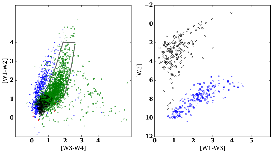
Figure 1: Left panel: WISE colour-colour diagram ([$W3$-$W4$] versus [$W1$-$W2$]), blue crosses and green circles denote verified O-rich and C-rich AGB catalogue of Suh & Kwon (2009, 2011). An empirical boundary ,the polygon, is used to select O-righ AGBs candidates. Black and red circles are our target sources. Red circles denote 9 Miras added at the late stage of the observational sessions. Right panel: WISE colour-magnitude diagram([$W1$-$W3$] versus $W3$) diagram. Blue squares are O-rich AGBs in the SMC selected based on the same colour-colour selection criteria. Black circles are 221 sources that have been observed by this survey.

Nikutta et al. (2014) and Lian et al. (2014) showed that the WISE colour-colour diagram ($W1$-$W2$ versus $W3$-$W4$) is effective at identifying O-rich and C-rich AGB stars. We therefore used this colour-colour diagram to select targets for this SiO maser survey. Firstly, we used the verified C-rich and O-rich AGBs catalogue of Suh & Kwon (2009, 2011), shown as blue pluses and green circles in the colour-colour diagram to define an empirical boundary (polygon in the colour-colour diagram) of O-righ AGBs (see the left panel of Fig. 1). Secondly, we used a colour-magnitude ([$W3$] versus [$W1$-$W3$]) diagram to remove contaminations, which are mainly extragalactic sources. In the right panel of Fig. 1, we show our observed target sources and O-rich AGB stars in the Small Magellanic Cloud (SMC). Using the colour-magnitude diagram, fainter extragalactic sources with locations below SMC AGBs are easily identified and excluded. Thirdly, we considered the following three constraints on the sky position, DEC. $>$ $-$25^∘ to be observable from the Nobeyma 45m telescope, Galactic latitude higher than 30^∘ to exclude Galactic plane contaminations, and angular separation $<$ 20^∘ from the Sgr stream orbital plane which follows a great circle with the normal vector towards l = 5.6^∘ b = $-$14.2^∘ (Majewski et al., 2003). We further checked the spectral type and stellar classifications with SIMBAD database to exclude tens of known C stars and galaxies. These criteria define a sample of 274 sources.

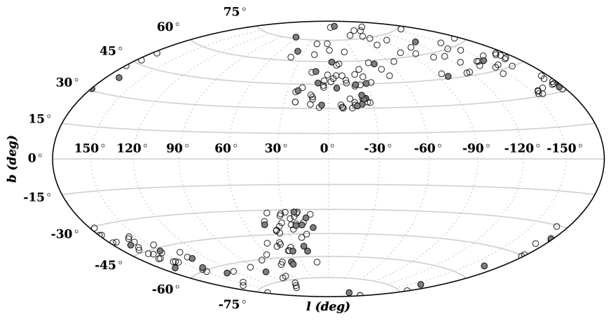
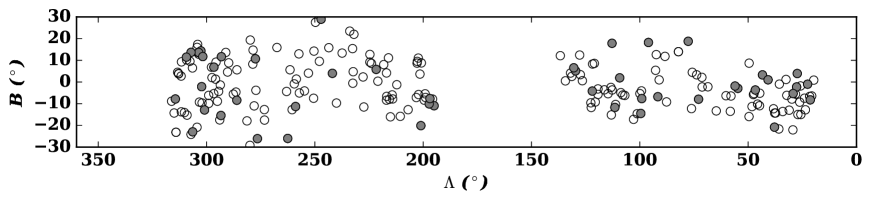
Figure 2: Top panel: Galactic distribution of observed targets, filled grey circles indicates sources with detection of SiO masers. Bottom panel: Same as top panel but in the Stellar Stream coordinate system.

Around 30 sources from our sample were not observed due to time constraints and conflict with the Solar position. In addition, considering the high detection rate of SiO masers in Miras, in the last stage of our observation sessions, we observed nine additional Miras which were just outside of our original selection polygon (red circles in Fig. 1). In total, we searched for SiO maser emission in 221 sources, including 108 (49%) Miras, 37 (17%) semi-regular stars, 23 (10%) long period variables, 42 (19%) stars and 11 (5%) other types, including 5 variable stars , 2 Infra-red sources, 2 Mira candidates, 1 S star and 1 long period Variable candidate. In Fig. 2, we show the locations of these sources in Galactic coordinates and Sgr stellar stream coordinates, where filled grey circles indicate sources with detections of maser emissions. The defination of the Sgr stellar stream coordinates can be found in Section 5.2.3 of Majewski et al. (2003), with the latitudes of Sgr stellar stream coordinates, $B$, defined by the Sgr debris projected on the sky as viewed from the Sun. The normal vector of the Sgr orbital plane is toward the direction of ($l$, $b$) = (273^∘.8, $-13^{\circ}$.5) and with $A$ = 0^∘ towards the center of the Sgr dSph. Equations to convert between the equatorial and the Sgr stream coordinate systems can be found in the appendix of Belokurov et al. (2014). Source details, i.e., source name (Galactic coordinate notation), equatorial coordinates, star type and spectral type are given in Table 8. For variable stars, Bayer designation names are also given, where star type and spectral type were queried from the SIMBAD database.

2.2 Observation

We carried out observations of the SiO v=1, 2, J=1-0 (43.122 and 42.820 GHz) transitions for 221 sources with the Nobeyama 45-m telescope in April and May of 2016. During observation sessions, pointing was checked every 2 hours using known sources of strong SiO maser emission. The half power beam width was 38.7^′′ at 43 GHz, with an aperture efficiency of 0.53. The backend was set with bandwidth of 125 MHz and channel spacing of 30.52 kHz, covering a velocity range of $\pm$430  km s^-1 with a velocity spacing of 0.21  km s^-1.

The data were calibrated using the chopper wheel method, which corrected for atmospheric attenuation and antenna gain variations to yield an antenna temperature $T^{\ast}_{A}$. System temperatures were within 150 to 230 K. The integration time per source was 10-30 minutes giving a 1$\sigma$ level of 0.03-0.05K. The conversion factor from the antenna temperature, $T^{\ast}_{A}$  in units of K, to flux density in units of Jy, was about 2.71Jy K^-1, which was estimated using an aperture efficiency of 0.53 and forward efficiency of 0.65.

3 Survey Results and SiO catalogue

3.1 Survey Results

Table 1: List of detections of SiO maser

ID	Source	Other	R.A.(J2000)	DEC.(J2000)	$V_{\rm LSR}$	Period	PLR Distance	WISE Distance
	Name	Name	(h:m:s)	(d:m:s)	(km s-1)	(day)	(kpc)	(kpc)
1	G004.482$+$32.104	BD Oph	16 05 46.29	$-$06 42 27.8	-8.8	340.440	2.003	2.791
2	G008.104$+$45.840	MW Ser	15 28 43.67	$+$03 49 43.6	41.0			1.659
3	G011.025$+$53.268	FV Boo	15 08 25.77	$+$09 36 18.4	4.5	313.500	1.990	1.821
4	G011.159$-$41.196	X Mic	21 04 36.85	$-$33 16 47.3	17.8	239.720	1.463	1.528
5	G015.405$-$35.139	R Mic	20 40 02.99	$-$28 47 31.2	19.9	138.620	0.765	1.212
6	G019.002$-$39.495	RR Cap	21 02 20.78	$-$27 05 14.9	-51.8	277.540	2.071	1.135
7	G019.509$-$56.308	R PsA	22 18 00.24	$-$29 36 13.8	-29.0	294.950	1.692	1.691
8	G021.513$-$53.023	S PsA	22 03 45.83	$-$28 03 04.2	-100.8	271.350	1.908	2.467
9	G022.158$+$40.858	U Ser	16 07 17.66	$+$09 55 52.5	-15.0	238.250	1.707	1.611
10	G022.943$-$31.448	RU Cap	20 32 34.16	$-$21 41 26.5	9.8	347.370	1.444	1.706
11	G023.376$-$39.816	V Cap	21 07 36.63	$-$23 55 13.4	-20.9	276.260	1.458	1.572
12	G038.070$+$66.469	R Boo	14 37 11.58	$+$26 44 11.7	-42.4	223.255	0.576	1.091
13	G045.734$-$38.770	HY Aqr	21 31 06.50	$-$07 34 20.4	26.3	311.350	3.026	3.718
14	G064.549$+$76.014	RT CVn	13 48 44.69	$+$33 43 34.2	26.3	253.600	3.651	4.738
15	G085.581$-$67.859	V Cet	23 57 54.07	$-$08 57 31.2	50.9	258.910	1.865	2.153
16	G131.720$-$64.091	Z Cet	01 06 45.20	$-$01 28 51.8	4.0	184.405	1.053	1.270
17	G133.797$-$53.388	S Psc	01 17 34.56	$+$08 55 52.0	4.3	404.620	0.941	1.246
18	G141.940$-$58.536	R Psc	01 30 38.35	$+$02 52 52.5	-57.0	345.250	0.958	1.484
19	G149.396$-$46.550	S Ari	02 04 37.67	$+$12 31 36.9	9.5	291.000	2.602	2.335
20	G165.616$-$40.899	YZ Ari	02 57 27.52	$+$11 18 05.3	13.0	447.000	2.691	2.635
21	G166.965$-$54.751	R Cet	02 26 02.31	$-$00 10 42.0	35.2	166.240	0.623	1.376
22	G168.980$+$37.738	X UMa	08 40 49.50	$+$50 08 11.9	-82.9	249.040	2.329	3.397
23	G179.379$+$30.743	—	08 05 03.70	$+$40 59 08.1	-10.6			3.344
24	G180.069$-$36.185	V1083 Tau	03 43 43.89	$+$06 55 30.5	58.0	343.000	3.322	4.451
25	G180.829$+$32.784	W Lyn	08 16 46.88	$+$40 07 53.3	-24.8	295.200	2.106	2.368
26	G182.006$-$35.653	V1191 Tau	03 49 27.68	$+$06 04 40.4	61.0	338.000	2.373	1.654
27	G183.614$+$31.966	RT Lyn	08 14 50.64	$+$37 40 11.7	27.5	394.600		1.616
28	G195.025$-$53.735	SS Eri	03 11 53.14	$-$11 52 32.4	33.2	316.700	3.065	3.334
29	G198.593$-$69.596	RY Cet	02 16 00.08	$-$20 31 10.5	-2.8	369.000	1.270	1.433
30	G211.919$+$50.661	V Leo	10 00 01.99	$+$21 15 43.9	-25.5	273.350	1.530	1.002
31	G235.246$+$67.258	TZ Leo	11 23 40.03	$+$16 51 07.0	12.9	327.750	0.795	1.122
32	G248.071$-$84.665	U Scl	01 11 36.38	$-$30 06 29.4	-10.3	333.730	1.771	2.436
33	G261.694$+$46.256	RT Crt	11 01 55.14	$-$07 39 41.8	32.9	263.100	2.032	3.177
34	G315.566$+$57.522	VY Vir	13 18 30.52	$-$04 41 03.2	72.0	278.520	1.579	2.133
35	G325.570$+$85.690	T Com	12 58 38.90	$+$23 08 21.0	26.1	406.000	1.838	1.875
36	G330.757$+$45.262	Z Vir	14 10 22.10	$-$13 18 11.8	66.8			3.022
37	G334.109$+$36.043	LY Lib	14 37 29.14	$-$20 19 41.2	-25.4	283.500	3.379	4.111
38	G335.504$+$35.524	SX Lib	14 42 46.26	$-$20 12 36.1	-31.2	331.450	1.952	1.842
39	G336.532$+$38.006	V Lib	14 40 22.18	$-$17 39 26.9	18.1	255.650	3.047	2.714
40	G337.373$+$32.451	EG Lib	14 55 21.62	$-$22 00 19.6	-7.8	386.000	1.312	1.805
41	G339.224$+$44.663	KS Lib	14 32 59.87	$-$10 56 03.2	70.7	375.500	3.788	3.076
42	G340.829$+$31.460	YY Lib	15 08 10.66	$-$21 10 00.3	-3.9	229.865	3.406	3.465
43	G353.826$+$42.588	Y Lib	15 11 41.26	$-$06 00 41.2	14.9	276.350	1.285	1.875
44	G356.642$+$59.618	AP Vir	14 28 30.27	$+$07 17 37.1	37.2	306.500	2.295	1.961
Note: Column 1 are ID of sources; Column 2 are Galactic coordinate notated source names; column 3 are Bayer designation
names of variables; column 4 and 5 are equatorial coordinates;column 6 are $V_{\rm LSR}$; column 7 are periods of
variables; column 8 and 9 are PLR and WISE distances.

In Table 1, we list the SiO masers detected in this survey. Of the 44 objects, 35 have no previous report of SiO masers. Apart from 1 infrared source (G179.370+30.743) and 2 Mira candidates (G011.025+53.268 and G353.826+42.588), all others are known as Miras. The detection rate of this SiO maser survey was 20% or 39% considering a Mira-only subsample. Table 12 details the observational results of the 44 SiO maser sources.

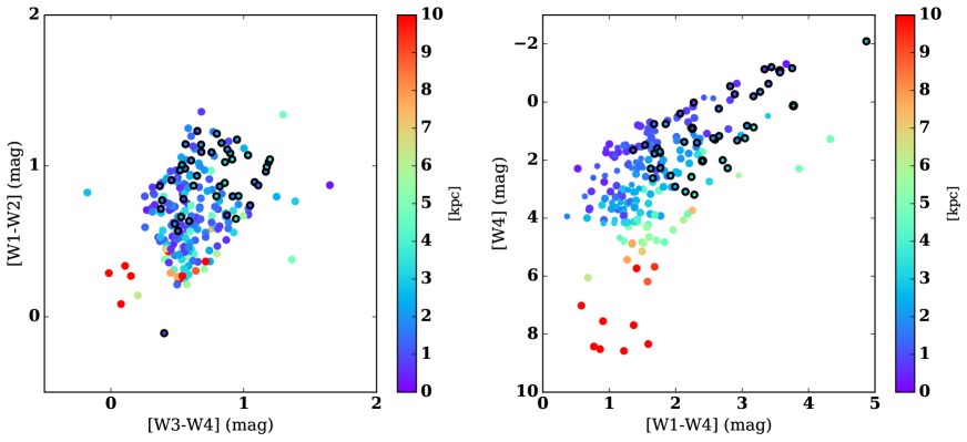
Figure 3: Left panel: WISE colour-colour ([$W3$-$W4$]V.S.[$W1$-$W2$]) diagram. Colors denote distances. With/without black edge circles denote our targets with/without SiO maser detections. Right panel: Symbols are same as left panel but for WISE colour-magnitude ([$W1$-$W4$]V.S.[$W4$]) diagram.

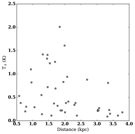
Figure 4: Distance versus SiO maser flux density in unit of antenna temperature.

Fig. 3 shows the colour-colour and colour-magnitude diagrams of our sample with/without maser detections. We found that the $W1$-$W4$ colour is higher than 1.3 for all SiO maser sources, thus presenting a suitable selection criteria for future AGB maser surveys. As indicated by colours of dots in Fig. 3, all the SiO masers detected by this survey are within 5 kpc. Methods used to derive distances are presented in Section 4.1.

In Fig. 4, we plot distances versus antenna temperatures of SiO v=1 J =1-0 maser emission. There is a trend that SiO maser line emission at near distances tend to be brighter than those of sources at further distances.

Table 2: Galactic SiO maser catalogue

ID	Source	R.A.(2000)	DEC.(2000)	$V_{\rm LSR}$	J	H	Ks	$W1$	$W2$	$W3$	$W4$	Period	Distance	Ref.
	Name	(h:m:s)	(d:m:s)	(km s-1)	(mag)	(mag)	(mag)	(mag)	(mag)	(mag)	(mag)	(day)	(kpc)
1	G108.713$-$35.564	00 00 06.6	25 53 11.3	-29.0	2.225	1.317	0.915	2.838	1.890	-0.615	-0.712	327.400	0.53/—	17
2	G116.144$-$06.556	00 03 21.3	55 40 50.0	-17.5	2.770	1.810	1.135	1.211	1.012	-0.958	-2.165	413.480	0.70/—	43
3	G116.145$-$06.557	00 03 21.6	55 40 48.0	2.0	2.770	1.810	1.135	1.211	1.012	-0.958	-2.165	413.480	—/—	6
4	G113.251$-$21.875	00 04 20.5	40 06 36.0	-91.0	3.570	2.592	2.084	2.315	1.504	0.560	0.171	313.000	—/1.07	6
5	G039.912$-$80.045	00 07 36.2	25 29 40.0	22.9	4.254	3.199	2.652	2.444	1.501	0.114	-0.606	411.000	1.39/1.43	43
6	G116.964$-$07.516	00 10 09.1	54 52 34.3	-35.2	4.822	3.747	3.043	2.683	1.762	1.425	0.745	396.000	1.63/1.20	46
Note: Column 1 are ID of sources; Column 2 are Galactic coordinate notated source names;; column 3 and 4 are equatorial coordinates; column 5 are $V_{\rm LSR}$;
olumn 6, 7, 8 are 2MASS J, H, Ks magnitudes; column 9,10, 11, 12 are WISE 4 bands magnitudes; column 13 are periods of variables; column 14 are PLR and
WISE distances; last column gives references. The full catalogue together with 48 references is present in online materials.

3.2 Galactic SiO maser survey catalogue

In order to identify potential SiO maser sources in the Sgr stellar stream, in addition to our observations, we compiled a Galactic SiO maser catalogue that includes $\sim$2300 sources from 48 papers published before 2017 (Table 2). These SiO masers were observed at transitions of v=0,1 J=1-0 (43/42 GHz) or v=0,J=2-1 (86 GHz). For sources which were reported in more than one papers, the mean $V_{\rm LSR}$ value was calculated.

The positional accuracy of the WISE point source catalogue is 0.5 ^′′. Regarding SiO masers surveys, aside from several blind surveys towards the Bugle and Galactic centre region (Shiki & Deguchi, 1997; Izumiura et al., 1998), and interferometric (JVLA &ATCA) surveys toward the Galactic centre region (Sjouwerman et al., 2002; Li et al., 2010), nearly all other surveys have samples selected from IRAS, 2MASS, MSX or variable star catalogues. Despite the majority of maser surveys being conducted with single dish observations with beam sizes $\sim$ 40 ^′′, the positional accuracy of most infrared selected sources is as good as 3 ^′′. When matching with the WISE point source catalogue, we used a search radius of 5 ^′′. We further removed extended sources and spurious sources, such as diffraction spikes and halos in nearby bright sources. Most sources without 2MASS or WISE conterparts are sources towards the Bulge and Galactic centre where high stellar densities result in source confusion. In summary, we have compiled a catalogue including $\sim$2300 SiO masers, and derived distances for $\sim$1000 of them. The full catalogue is included in the online material.

4 Discussions

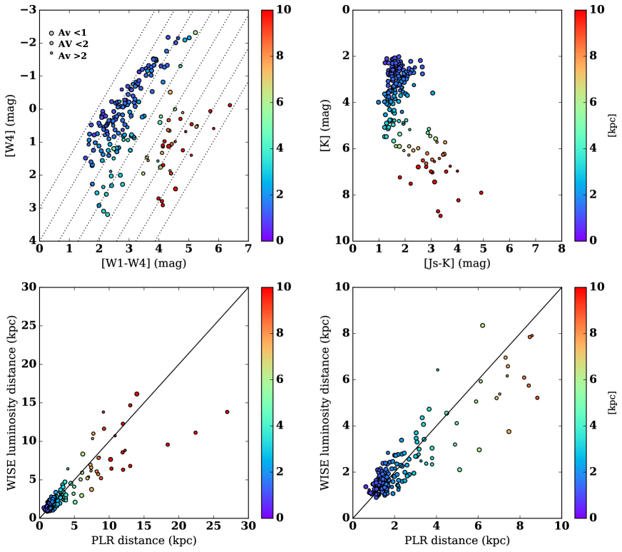
Figure 5: Top Left panel: WISE colour-magnitude ([$W1$-$W4$] VS [$W4$]) diagram, with colour of symbols denotes distances and size of symbols denotes interstellar extinction.Top Right panel: 2MASS colour-magnitude ([Js]-[K] VS [K]). Bottom Left panel: PLR distances versus WISE luminosity distances. Bottom Right panel: sample as bottom left panel, but with a zoom on inner 10 kpc range.

4.1 Distance and Galactic distribution

Distance is a key parameter in investigations of the distribution of Galactic objects (Honma et al., 2012; Reid et al., 2014; Bland-Hawthorn & Gerhard, 2016). For SiO masers in Miras with known periods and Ks magnitudes, their distances can be calculated via the period luminosity relation (PLR). Formulas used to derive the PLR distances are given in Appendix A.1.

In the top panel of Fig. 5, we present the WISE and 2MASS colour-magnitude diagram of O-rich Miras in our combined catalogue. In the WISE [$W1$-$W4$] versus [$W4$] diagram, a clear gradient of distances from the top left to the bottom right direction can be seen. Redder sources tend to be brighter at $W4$ band due to reddening by the circumstellar dusty envelope. As described in Appendix A.2, by using Miras with known PLR distances, we derived an empirical relation to derive the distance based on the WISE [$W1$-$W4$] colour and [$W4$] magnitude for O-rich Miras (Equation 12). The details on the derivation and calibration of this relationship is given in appendix A.2. This relation can be used to estimate WISE luminosity distances of O-rich Miras without known periods or Ks magnitudes. In the lower panels of Fig. 5, we plot the WISE distances against the PLR distances for Miras with both distances. The mean and standard deviation of $D_{WISE}$-$D_{PLR}$ is $-$0.26 and 1.6 kpc. Generally, distances estimated by these two methods agree within 2 kpc. Most large deviations are sources towards the Bulge and Galactocentrc region where interstellar extinction is high (Av $>$ 2). In summary, we obtained PLR distances for 587 sources and WISE distances for 749 sources.

In Fig. 6, we show histograms of heliocentric distances and distances from the Galactic plane. The majority of PLR distances are within 5 kpc. This is due to high extinction at further distances. In contrast, there are only a few sources with the WISE distances within 2 kpc. This is due to the saturation of WISE phototmetry for nearby AGBs.

With these distances, we estimated a Galactic plane scale height of 0.40 kpc for Miras with SiO masers, by fitting the histogram of Galactic plane distances with an exponential density profile(right panel of Fig. 6). When estimating the scale height, only sources with distances smaller than 7 kpc were used, given that distance uncertainties of sources towards the Bulge and Galactocentric region tend to be large (Fig. 5 and Fig. 7). It should be mentioned that more than half of the SiO masers are located within 3 kpc of the Sun, as can be seen in Fig. 6 and Fig. 7, so that the scale height of 0.40 kpc we estimated here can be an average scale height of O-rich AGBs around 3 kpc of the sun.

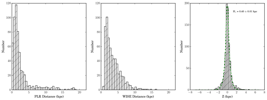
Figure 6: Left and middle panels are histograms of PLR distances and WISE distances. Right panel is the histogram of Galactic plane distances. The green dash line denotes the fitted exponential density profile, with a scale height of 0.40 kpc.

In Fig. 7 we present the locations of these SiO masers in the Galaxy. We identified 42 off-plane sources with Galactic plane distances higher than 1.2 kpc, which are listed in Table 3 and highlighted in Fig. 7. Around 50% of these off-plane SiO maser were found by this survey.

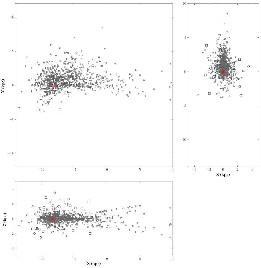
Figure 7: 3D locations of SiO masers in the Galactocentric Cartesian coordinates, with the Galactic centre at the zero point and the Sun at [$-$8.34, 0, 0] kpc. Squares denote sources with PLR distances and circles denote sources with WISE luminosity distances. In $XZ$ plot, large symbols denote off-plane SiO masers. Circles denote sources detected by this survey, Squares denote sources from published references.

Table 3: Off plane SiO masers

ID	Source	R.A.(2000)	DEC.(2000)	$V_{\rm LSR}$	Period	PLR Distances	WISE Distances	$Z$	Ref.
	Name	(h:m:s)	(d:m:s)	(km s-1)	(day)	(kpc)	(kpc)	(kpc)
1	G039.912$-$80.045	00 07 36.2	$-$25 29 40.0	22.9	411.000	1.39	1.43	-1.37	8
2	G248.071$-$84.665	01 11 36.4	$-$30 06 29.4	-10.3	333.730	1.77	2.44	-1.76	1
3	G149.396$-$46.550	02 04 37.7	12 31 36.9	9.5	291.000		2.34	-1.70	1
4	G165.616$-$40.899	02 57 27.5	11 18 05.2	14.2	447.000	2.69	2.63	-1.76	1, 2
5	G195.025$-$53.735	03 11 53.1	$-$11 52 32.4	33.2	316.700	3.07	3.33	-2.48	1
6	G180.069$-$36.185	03 43 43.9	06 55 30.5	58.0	343.000	3.32	4.45	-1.96	1
7	G182.006$-$35.653	03 49 27.7	$+$06 04 40.4	61.0	338.000	2.37	1.65	-1.38	1
8	G174.233$-$28.113	03 54 23.6	$+$16 01 01.9	45.5	334.500	2.70	1.96	-1.27	2
9	G195.134$-$24.895	04 50 57.3	$+$03 08 32.3	-13.2	358.500	2.92	1.97	-1.23	2
10	G195.853$-$23.965	04 55 30.3	$+$03 04 28.1	47.0	396.000	3.37	3.45	-1.37	2
11	G238.258$-$26.921	05 47 58.7	$-$33 05 10.9	110.8	199.300	4.21	7.27	-1.91	3
12	G179.379$+$30.743	08 05 03.7	40 59 08.1	-9.8			3.34	1.71	1, 4
13	G168.980$+$37.738	08 40 49.6	50 08 12.1	-82.9	249.040	2.33	3.40	1.43	1
14	G190.023$+$51.458	09 53 43.5	34 55 32.0	-11.0	233.830		2.00	1.56	5
15	G261.694$+$46.256	11 01 55.1	$-$07 39 41.9	32.9	263.100		3.18	2.30	1
16	G170.681$+$71.517	11 41 40.3	38 28 29.3	-56.3	252.460	3.03	3.48	2.87	3
17	G288.878$+$34.294	11 59 19.1	$-$27 09 03.5	72.5	301.000	4.49	4.59	2.53	4
18	G282.845$+$50.684	12 00 20.8	$-$10 11 04.9	-4.3	294.765	1.69	1.70	1.31	2
19	G248.033$+$76.318	12 04 15.5	18 47 00.0	-4.0			1.64	1.59	5
20	G325.570$+$85.690	12 58 38.9	23 08 21.1	27.0	406.000	1.84	1.88	1.83	1, 6
21	G315.565$+$57.522	13 18 30.4	$-$04 41 05.1	72.0	278.520	1.58	2.13	1.33	1
22	G064.549$+$76.014	13 48 44.7	33 43 34.3	26.3	253.600	3.65	4.74	3.54	1
23	G330.755$+$45.262	14 10 21.4	$-$13 18 14.8	66.8	304.105	3.17	3.02	2.25	1
24	G356.642$+$59.618	14 28 30.3	07 17 37.1	37.2	306.500		1.96	1.69	1
25	G339.224$+$44.663	14 32 59.9	$-$10 56 03.4	69.2	375.500	3.79	3.08	2.66	1, 4
26	G334.109$+$36.043	14 37 29.1	$-$20 19 41.2	-25.4	283.500	3.38	4.11	1.99	1
27	G336.532$+$38.006	14 40 22.2	$-$17 39 26.9	18.1	255.650	3.05	2.71	1.88	1
28	G340.829$+$31.460	15 08 10.6	$-$21 10 00.3	-3.9	229.865	3.41	3.46	1.78	1
29	G011.025$+$53.268	15 08 25.8	09 36 18.3	6.8	313.500	1.99	1.82	1.59	1, 4
20	G011.025$+$53.268	15 08 25.8	09 36 18.4	-10.2	313.500	1.99	1.82	1.59	7, 8
31	G066.876$+$47.996	16 05 28.9	42 10 29.4	0.3			1.97	1.46	4
32	G003.227$+$22.945	16 32 24.6	$-$13 12 01.3	-28.4	332.000		3.83	1.49	9
33	G007.656$+$18.016	16 58 46.7	$-$12 43 46.9	-62.7			4.79	1.48	2
34	G018.305$+$21.632	17 08 10.3	$-$02 20 22.6	-40.4			6.19	2.28	4
35	G008.400$-$18.623	19 19 09.6	$-$29 43 18.0	33.7			6.16	-1.97	7
36	G012.358$-$25.239	19 53 21.8	$-$28 30 39.0	-16.7	343.000	3.62	4.42	-1.54	7
37	G019.002$-$39.495	21 02 20.8	$-$27 05 14.7	-51.8	277.540	2.07	1.13	-1.32	1
38	G058.520$-$26.960	21 14 29.6	07 48 33.7	28.6	429.000		5.08	-2.30	2
39	G045.734$-$38.770	21 31 06.5	$-$07 34 20.4	26.3	311.350	3.03	3.72	-1.90	1
40	G021.513$-$53.023	22 03 45.8	$-$28 03 03.3	-100.8	271.350	1.91	2.47	-1.53	1
41	G019.509$-$56.308	22 18 00.2	$-$29 36 13.5	-29.0	294.950	1.69	1.69	-1.41	1
42	G085.581$-$67.859	23 57 54.1	$-$08 57 31.2	50.9	258.910	1.86	2.15	-1.72	1
Note: Column 1 are ID of sources; Column 2 are Galactic coordinate notated source names; column 3 and 4 are equatorial coordinates;
column 5 are $V_{\rm LSR}$; column 6 are periods of variables; column 7 and 8 are PLR and WISE distances; column 9 are off plane distances;
column 10 denote references.
Reference: (1) this paper; (2) Deguchi et al. (2012); (3) Deguchi et al. (2007);(4) Ita et al. (2001) (5) Benson et al. (1990);
(6) Deguchi et al. (2010); (7) Deguchi et al. (2004) (8) Kim et al. (2010); (9) Matsunaga et al. (2005)

4.2 Kinematics

The Galactic distribution shown in Fig. 7 indicates that the majority of Galactic SiO maser sources are within the Galactic disc. Regarding the off-plane SiO sources listed in Table 3, we test in this section whether these are halo/stream stars or thick-disc stars based on comparison of their line of sight velocities and those predicted by disc star models.

For disc stars, it is well known that late-type stars with higher velocity dispersions tend to have slower Galactocentric rotational speeds. This phenomenon is called “asymmetric drift” (Dehnen & Binney, 1998). Pasetto et al. (2012) studied the kinematics of thick disc stars as part of the RAdial Velocity Experiment (RAVE) and derived a rotational lag of 49$\pm$6  km s^-1 with respect to the LSR. Tian et al. (2015) determined the Solar motion using LAMOST DR1 data, and found a $\sim$3  km s^-1 asymmetric motion of stars with $T_{eff}<$6000 $K$ with respect to stars with $T_{eff}>$6000 $K$. Before investigating the kinematics of off-plane sources, we first studied the circular rotational speed and asymmetric drift of disc O-rich Miras.

Table 4: Variables used in kinematic analysis

Variables	Definitions
$D$	heliocentric distance
$R$	Galactocentric distance
$X$,$Y$,$Z$	Galactocentric Cartesian coordinates
$R_{0}$	Galactocentric radius of the Sun
$\Theta_{0}$	rotation velocity of the $\rm LSR$ around the Galactic centre
$U_{\odot}$, $V_{\odot}$, $W_{\odot}$,	velocity of the Sun with respect to the $\rm LSR$
$\Theta$	mean rotation velocity of stars around the Galactic centre
$\overline{U_{s}}$, $\overline{V_{s}}$, $\overline{W_{s}}$	peculiar (non-circular) motion of stars in cylindrical Galactocentric coordinates
$V_{\rm LSR}$	line-of-sight velocity of stars with respect to the $\rm LSR$
$V_{\rm helio}$	heliocentric line-of-sight velocity of stars
$V_{\rm obs}$	observed heliocentric line-of-sight velocity of stars
$V_{\rm model}$	heliocentric line-of-sight velocity of stars calculated by model
$S$	dispersion of heliocentric line-of-sight velocity (Eq. 3)

Table 5: velocity dispersion and mean velocity of $R$-$Z$ binned groups.

$Z$(kpc)	$R$(kpc)	Number	S	$\Theta+\overline{V_{s}}$	$\overline{U_{s}}$	$\overline{W_{s}}$	ID
			( km s-1)	( km s-1)	( km s-1)	( km s-1)
-0.1 $<Z<$ +0.1	+5.0 $<R<$ +9.0	192	+44.8 $\pm$ 1.1	+236.7 $\pm$ 7.6	-9.6 $\pm$ 6.2	+3.9 $\pm$ 10.7
-0.3 $<Z<$ -0.1	+5.0 $<R<$ +9.0	82	+36.6 $\pm$ 0.7	+225.2 $\pm$ 6.1	+6.7 $\pm$ 6.2	-7.8 $\pm$ 8.6
+0.1 $<Z<$ +0.3	+5.0 $<R<$ +9.0	100	+34.4 $\pm$ 0.6	+215.4 $\pm$ 5.6	+3.1 $\pm$ 6.5	+7.6 $\pm$ 8.5
-0.5 $<Z<$ -0.3	+5.0 $<R<$ +9.0	47	+31.9 $\pm$ 0.9	+220.1 $\pm$ 5.3	-4.7 $\pm$ 7.0	-15.3 $\pm$ 7.3
+0.3 $<Z<$ +0.5	+5.0 $<R<$ +9.0	67	+37.4 $\pm$ 1.0	+217.1 $\pm$ 6.6	-13.8 $\pm$ 5.7	+10.1 $\pm$ 8.3
-0.8 $<Z<$ -0.5	+5.0 $<R<$ +9.0	33	+36.4 $\pm$ 0.7	+217.4 $\pm$ 6.7	-11.9 $\pm$ 6.0	-5.3 $\pm$ 7.7
+0.5 $<Z<$ +0.8	+5.0 $<R<$ +9.0	56	+35.2 $\pm$ 1.0	+213.3 $\pm$ 6.5	-11.4 $\pm$ 6.5	+1.1 $\pm$ 7.7
+0.8 $<Z<$ +1.4	+5.0 $<R<$ +9.0	34	+39.8 $\pm$ 0.6	+208.5 $\pm$ 7.7	-2.8 $\pm$ 6.9	+2.0 $\pm$ 7.2
-1.4 $<Z<$ -0.8	+5.0 $<R<$ +9.0	23	+34.5 $\pm$ 1.6	+225.7 $\pm$ 8.3	-4.8 $\pm$ 6.8	+18.9 $\pm$ 6.4	3
+1.4 $<Z<$ +2.5	+5.0 $<R<$ +9.0	20	+33.3 $\pm$ 3.8	+189.9 $\pm$ 8.9	-12.2 $\pm$ 7.9	+33.6 $\pm$ 5.9	A
-0.1 $<Z<$ +0.1	+9.0 $<R<$ +15.0	32	+24.5 $\pm$ 0.9	+209.8 $\pm$ 6.5	-5.1 $\pm$ 4.2	-4.1 $\pm$ 11.1
+0.1 $<Z<$ +0.3	+9.0 $<R<$ +15.0	24	+25.7 $\pm$ 1.0	+213.0 $\pm$ 6.2	+7.3 $\pm$ 5.0	+3.1 $\pm$ 12.6
-0.3 $<Z<$ -0.1	+9.0 $<R<$ +15.0	21	+24.1 $\pm$ 0.8	+214.5 $\pm$ 6.0	+2.9 $\pm$ 4.8	-36.5 $\pm$ 19.1
+0.3 $<Z<$ +0.5	+9.0 $<R<$ +15.0	19	+30.1 $\pm$ 2.3	+214.3 $\pm$ 8.1	+35.1 $\pm$ 11.9	+112.3 $\pm$ 31.8	1
-0.5 $<Z<$ -0.3	+9.0 $<R<$ +15.0	19	+35.5 $\pm$ 1.1	+190.8 $\pm$ 8.3	+17.2 $\pm$ 6.5	-33.6 $\pm$ 17.8
+0.5 $<Z<$ +0.8	+9.0 $<R<$ +15.0	23	+35.2 $\pm$ 1.7	+235.5 $\pm$ 7.0	-9.4 $\pm$ 6.3	+9.4 $\pm$ 10.2
-0.8 $<Z<$ -0.5	+9.0 $<R<$ +15.0	12	+29.6 $\pm$ 5.7	+199.6 $\pm$ 7.3	-71.5 $\pm$ 9.6	+175.3 $\pm$ 21.8	2
-0.8 $<Z<$ -0.3	+9.0 $<R<$ +15.0	27	+36.1 $\pm$ 0.9	+201.1 $\pm$ 7.8	-2.9 $\pm$ 5.5	+33.6 $\pm$ 10.6
+0.3 $<Z<$ +0.8	+9.0 $<R<$ +15.0	38	+32.4 $\pm$ 0.8	+227.8 $\pm$ 7.0	+13.4 $\pm$ 6.8	+43.7 $\pm$ 14.0	C
-2.0 $<Z<$ -0.8	+9.0 $<R<$ +15.0	18	+39.7 $\pm$ 2.3	+176.0 $\pm$ 13.0	+25.2 $\pm$ 9.3	-54.3 $\pm$ 11.0	B
+0.8 $<Z<$ +2.0	+9.0 $<R<$ +15.0	15	+31.7 $\pm$ 3.1	+219.8 $\pm$ 8.3	+16.1 $\pm$ 7.3	-21.3 $\pm$ 8.3
Note: column 1 and 2 are binned ranges of $R$ and $Z$; column 3 are numbers of sources in $R$-$Z$ binned regions;
column 4 to 7 are S, $\overline{U_{s}}$, $\Theta$+$\overline{V_{s}}$, $\overline{W_{s}}$. The last column gives IDs of moving groups and high-speed stars.

Table 6: Source list of the northern (group A) and southern (group B) off-plane moving groups

ID	Source	Other	R.A.(J2000)	DEC.(J2000)	$V_{\rm LSR}$	$\Lambda_{\odot}$	$B_{\odot}$	$V_{GSR}$	Period	PLR Distance	WISE Distance
	Name	Name	(h:m:s)	(d:m:s)	(km s-1)	($\degr$)	($\degr$)	(km s-1)	(day)	(kpc)	(kpc)
1	G248.033+76.318	R Com	12 04 15.5	18 47 00.0	-4.0	249.84	-1.65	-52.3			1.64
2	G288.878+34.294	V0450 Hya	11 59 19.1	-27 09 03.5	72.5	273.40	+39.65	-99.5	301.0	4.49	4.59
3	G286.549+55.660	T Vir	12 14 36.7	-06 02 08.9	6.6	263.98	+19.58	-112.4	339.5	1.39	2.04
4	G325.570+85.690	T Com	12 58 38.9	23 08 21.1	27.0	258.91	-11.29	17.7	406.0	1.84	1.88
5	G315.565+57.522	VY Vir	13 18 30.4	-04 41 05.1	72.0	277.45	+10.70	-10.7	278.5	1.58	2.13
6	G064.549+76.014	RT CVn	13 48 44.7	33 43 34.3	26.3	262.52	-26.00	74.3	253.6	3.65	4.74
7	G330.755+45.262	Z Vir	14 10 21.4	-13 18 14.8	66.8	293.15	+11.66	-8.9	304.1	3.17	3.02
8	G334.779+50.121	IO Vir	14 11 17.6	-07 44 49.8	-26.8	290.35	+6.77	-86.9	500.0	2.46
9	G325.327+25.630		14 28 09.3	-33 00 03.4	-19.5	308.26	+26.02	-132.3	454.0	6.46
10	G356.642+59.618	AP Vir	14 28 30.3	07 17 37.1	37.2	286.03	-8.40	30.7	306.5		1.96
11	G339.224+44.663	KS Lib	14 32 59.9	-10 56 03.4	69.2	296.61	+6.84	13.7	375.5	3.79	3.08
12	G334.109+36.043	LY Lib	14 37 29.1	-20 19 41.2	-25.4	302.61	+14.34	-103.1	283.5	3.38	4.11
13	G336.532+38.006	V Lib	14 40 22.2	-17 39 26.9	18.1	301.74	+11.72	-50.9	255.6	3.05	2.71
14	G340.829+31.460	YY Lib	15 08 10.6	-21 10 00.3	-3.9	309.29	+11.46	-65.5	229.9	3.41	3.46
15	G011.025+53.268	FV Boo	15 08 25.8	09 36 18.3	6.8	293.35	-15.42	32.0	313.5	1.99	1.82
16	G066.876+47.996	V1012 Her	16 05 28.9	42 10 29.4	0.3	281.55	-49.51	135.7			1.97
17	G004.482+32.104	BD Oph	16 05 46.3	-06 42 27.8	-7.5	314.40	-7.82	7.1	340.4	2.00	2.79
18	G056.375+43.529	V0697 Her	16 27 51.4	34 48 10.5	54.5	293.92	-46.80	187.3	486.0	1.47	2.14
19	G003.227+22.945	V0720 Oph	16 32 24.6	-13 12 01.3	-28.4	323.25	-4.73	-17.0	332.0		3.83
1	G128.642-50.107	WX Psc	01 06 26.0	12 35 53.0	7.5	99.17	-19.03	117.7	660.0	1.59
2	G141.939-58.536	R Psc	01 30 38.3	02 52 53.0	-57.5	99.10	-7.64	13.3	345.2	0.96	1.48
3	G149.396-46.550	S Ari	02 04 37.7	12 31 36.9	9.5	111.52	-11.71	86.5	291.0		2.34
4	G166.966-54.751	R Cet	02 26 02.3	-00 10 42.0	37.0	109.29	+1.92	65.6	166.2	0.62	1.38
5	G146.989-21.317	TV Per	02 43 48.5	36 15 02.0	-25.4	133.26	-26.89	86.3	358.0	1.35	2.30
6	G161.474-41.919	RU Ari	02 44 45.5	12 19 02.9	20.4	119.81	-6.59	72.4	353.5	1.23
7	G165.616-40.899	YZ Ari	02 57 27.5	11 18 05.2	14.2	121.94	-4.18	55.5	447.0	2.69	2.63
8	G195.025-53.735	SS Eri	03 11 53.1	-11 52 32.4	33.2	112.84	+17.83	-0.5	316.7	3.07	3.33
9	G180.069-36.185	V1083 Tau	03 43 43.9	06 55 30.5	58.0	129.65	+5.13	57.8	343.0	3.32	4.45
10	G182.006-35.653	V1191 Tau	03 49 27.7	06 04 40.4	61.0	130.49	+6.54	54.7	338.0	2.37	1.65
11	G174.233-28.113	UY Tau	03 54 23.6	16 01 01.9	45.5	136.30	-1.79	65.0	334.5	2.70	1.96
12	G206.048-43.665	WZ Eri	04 02 08.7	-13 44 56.0	9.4	123.05	+25.71	-60.5	401.5	1.47
13	G195.134-24.895	EP Ori	04 50 57.3	03 08 32.3	-13.2	143.16	+15.89	-65.3	358.5	2.92	1.97
14	G195.853-23.965	V1648 Ori	04 55 30.3	03 04 28.1	47.0	144.21	+16.41	-7.9	396.0	3.37	3.45
15	G227.912-25.120	RT Lep	05 42 33.2	-23 41 41.0	65.2	142.94	+46.20	-82.6	400.0	1.12	3.43
16	G238.258-26.921		05 47 58.7	-33 05 10.9	110.8	137.14	+55.22	-56.0	199.3	4.21	7.27
Note: Column 1 are ID of sources; Column 2 are Galactic coordinate notated source names; column 3 are Bayer designation names of variables; column 4 and 5
are equatorial coordinates; column 6 are $V_{\rm LSR}$; column 7, 8 are Sgr stellar stream coordinates; column 9 are radial velocities with respect to the Galactic centre;
column 10 are periods of variables; column 11and 12 are PLR and WISE distances.

Table 7: List of very high speed Sources

Source	Other	R.A.(J2000)	DEC.(J2000)	$V_{\rm LSR}$	Period	PLR Distance	WISE Distance	ID
Name	Name	(h:m:s)	(d:m:s)	(km s-1)	(day)	(kpc)	(kpc)
G002.216-37.218	RV Mic	20 40 29.9	$-$39 37 42.0	-96.55	327.0		2.29	1
G196.675+21.331	S Gem	07 43 02.5	$+$23 26 58.2	94.8	292.1	1.41	1.14	2
G138.089-26.921	T Tri	01 56 47.1	$+$34 01 10.7	-121.9	324.0	1.60	1.87	3

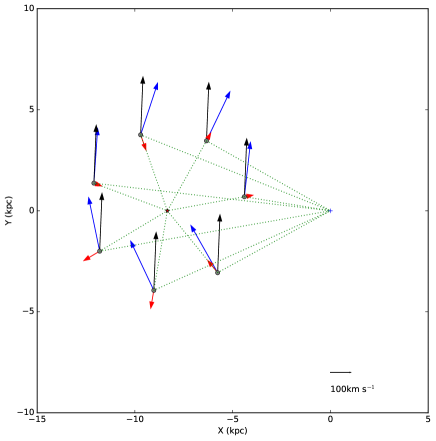
Figure 8: Sketch of de-projection of the line-of-sight velocity. Blue and black arrows are velocity vectors of stars and the Sun with respect to the Galactic centre. Red arrows denote the line of sight velocities of stars with respect to the Sun.

The de-projection method is a useful method to study Galactic kinematics using radial velocity data (Pasetto et al., 2012; Tian et al., 2015). Here we used a similar de-projection method to model the $V_{\rm LSR}$ of SiO masers. A sketch of the de-projection is shown in Fig. 8, where, blue and black arrows are velocity vectors of the star ($\overrightarrow{V_{\star}}$) and the Sun ($\overrightarrow{V_{\odot}}$) with respect to the Galactic centre. The line of sight velocity of the star towards the Sun, V_helio, denoted by the red arrow, is the projection of ($\overrightarrow{V_{\star}}$-$\overrightarrow{V_{\odot}}$) on $\overrightarrow{r_{\star}}$, where $\overrightarrow{r_{\star}}$ is the direction vector from the Sun towards the star (Equation 1). The observed $V_{\rm LSR}$ can be converted to V_helio by adding back the component of the standard Solar motion in the line-of-sight direction that had been removed from the observed Doppler shift to calculate $V_{\rm LSR}$ using Equation 2, where (U${}^{Std}_{\odot}$, V${}^{Std}_{\odot}$, W${}^{Std}_{\odot}$) are not the best values available today, but the (old) standard Solar motion, a value of 20 km s^-1 toward $\alpha$(1900) = 18^h, $\delta$(1900) = +30^d generally adopted by observatories (Reid et al., 2014). In this study, for values of the Solar motion and Galactic parameters, we adopted the A5 model from Reid et al. (2014), where (U_⊙, V_⊙,W_⊙)= (10.7$\pm$1.8, 15.6$\pm$6.8, 8.9$\pm$0.9)  km s^-1, $\Theta_{0}$ = 240$\pm$8  km s^-1 and $R_{0}$ = 8.34 kpc.

For modelling radial velocities, we assumed that a group of stars with similar Galactic locations (similar $R$ and $Z$) share a mean 3D velocity of $\overrightarrow{V_{\star}}$ = ($\overline{U_{s}}$,$\Theta$+$\overline{V_{s}}$, $\overline{W_{s}}$) with respect to the Galactic centre, where ($\overline{U_{s}}$, $\overline{V_{s}}$, $\overline{W_{s}}$) are peculiar velocities in the direction of the Galactic centre, Galactic rotation and toward the North Galactic Pole (NGP), $\Theta$ is the mean circular rotational velocity. For the Sun, $\overrightarrow{V_{\odot}}$ = ($U_{\odot}$,$\Theta_{0}$+$V_{\odot}$, $W_{\odot}$). It is noted that the, $\overline{V_{s}}$ and $\Theta$ are two highly correlated parameters, which can not be separated. Instead, $\Theta$+$\overline{V_{s}}$ can be well constrained, as have been pointed out by several previous studies (McMillan & Binney, 2010; Honma et al., 2012; Reid et al., 2014). Thus, in our study, we treat $\Theta$+$\overline{V_{s}}$ as one parameter that we need to fit.

$$V_{\rm helio}=V_{\rm model}=(\overrightarrow{V_{\star}}-\overrightarrow{V_{\odot}})\cdot\overrightarrow{r_{\star}}$$ (1)

$$V_{\rm helio}=V_{\rm obs}=V_{\rm LSR}-(\textit{U}^{Std}_{\odot}~{}\mathrm{cos}~{}\textit{l}~{}+\textit{V}^{Std}_{\odot}~{}\mathrm{sin}~{}\textit{l})\mathrm{cos}~{}\textit{b}-\textit{W}^{Std}_{\odot}~{}\mathrm{sin}~{}\textit{b}$$ (2)

$$S^{2}=\frac{\sum(V_{\rm obs}-V_{\rm model})^{2}}{N}$$ (3)

A program was developed for investigating kinematics with (l,b,D,$V_{\rm LSR}$) of a group of stars as inputs and (S, $\overline{U_{s}}$, $\Theta$+$\overline{V_{s}}$, $\overline{W_{s}}$) of the group as outputs. S denotes the dispersion of the line-of-sight velocity, which is expressed in Equation 3. We used the Markov Chain Monte Carlo (MCMC) method in the procedure to minimize the dispersion and estimate the uncertainties of (S, $\overline{U_{s}}$, $\Theta$+$\overline{V_{s}}$, $\overline{W_{s}}$). We first calculate a prior $S$, by using a prior of ($\overline{U_{s}}$, $\Theta$+$\overline{V_{s}}$, $\overline{W_{s}}$)=(0, 220, 0)  km s^-1. Then we let ($\overline{U_{s}}$, $\Theta$+$\overline{V_{s}}$, $\overline{W_{s}}$) walk randomly in an sampling window of (30, 30, 30)  km s^-1 to calculate a posterior $S$ until we find better solution of ($\overline{U_{s}}$, $\Theta$+$\overline{V_{s}}$, $\overline{W_{s}}$) with smaller $S$. Once a better solution is found, we use these values to replace the prior, and resample again to search for better solutions. Usually, $S$ can converge within 10 interations. When S converges, ($\overline{U_{s}}$, $\Theta$+$\overline{V_{s}}$, $\overline{W_{s}}$) and $S$ are recorded and the program stops. We repeat the above s 10000 times, and estimate the mean and standard deviation of ($\overline{U_{s}}$, $\Theta$+$\overline{V_{s}}$, $\overline{W_{s}}$) and $S$ as the final outputs.

Using this procedure, we obtained the values of $\Theta$+$\overline{V_{s}}$ = 225.6  km s^-1, $S$ = 34.1  km s^-1 for disc sources with $D<$ 1.2 kpc; and $\Theta$+$\overline{V_{s}}$ = 185.4  km s^-1, $S$ = 41.3  km s^-1 for off-plane ($Z>$ 1.2 kpc) sources. Adopting $\Theta_{0}$ = 240  km s^-1, the velocity lag of disc and off-plane SiO masers with respect to the $\rm LSR$ are 15  km s^-1 and 55  km s^-1 respectively.

4.3 Moving groups and high speed stars

With the aim of identifying potential stream motions and/or high-speed sources, we further apply this procedure to a series of ($R$,$Z$)-binned subsamples. The ranges of ($R$, $Z$) bins are given in Table 5. Regarding the group strategy, we initially separated $R>$ 9 and $R<$ 9 sources into two groups, since (1) sources are not uniformly distributed in the Galactic plane; there are fewer sources outside of $R>9$ kpc, and (2) the relatively large uncertainties in the rotation curve at $R>$ 9kpc (Nakashima et al., 2000; Demers & Battinelli, 2007; Xin & Zheng, 2013). We only consider sources with $R>5$ kpc, since (1) the kinematics in the inner disc could not be well modeled by circular motions due to the influence of the Galactic bar; (2) distance uncertainties for sources with $R<$ 5kpc tend to be high (Fig. 5 and Fig. 7).

Outputs for each of the $R$-$Z$ binned groups obtained with the above procedures are listed in Table 5 and visualized in Fig. 9. Top panels plot how (S, $\overline{U_{s}}$, $\Theta$+$\overline{V_{s}}$, $\overline{W_{s}}$) varies with $Z$ for sources with 5 $<R<$ 9 kpc, while bottom panels plot the same but for sources at $R>$9 kpc. Horizonal “errorbars” indicate the min($Z$) and max($Z$) of stars in the binned range of $Z$; vertical errorbars show 1$\sigma$ uncertainties of $S$, $\Theta+\overline{V_{s}}$, $\overline{U_{s}}$, $\overline{W_{s}}$. Figure 9 is very useful for identifying potential stream motions and/or high velocity stars. Careful inspection of these diagrams allows us to identify three bulk motions and three very high speed stars.

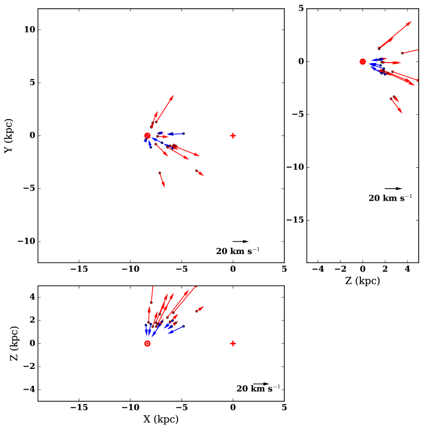
Figure 10: 2D Projection of $V_{\rm obs}$-$V_{\rm model}$ in Galactocentric Cartesian coordinate for group A, with 5 $<R<$ 9 kpc, 1.4 $<Z<$ 2.5 kpc. $V_{\rm model}$ was calculated by using a rotational speed of 180  km s^-1. Blue/red arrows denote negative/positive $V_{\rm obs}$-$V_{\rm model}$.

In the top panels of Fig. 9, for the 5 $<R<$ 9 kpc, 1.4 $<Z<$ 2.5 kpc group, one can see large deviations of $\overline{W_{s}}$ and $\Theta$+$\overline{V_{s}}$, and a very large uncertainty in S. Further inspection of $V_{\rm obs}$-$V_{\rm model}$ (Fig. 10) reveals the bulk motion of this group. For further discussion, we denote this group as group A. In Fig. 10, dots with arrows denote the 2D projection of $V_{\rm obs}$-$V_{\rm model}$, where a model with a rotational speed of 180  km s^-1 was used. Blue/red colours denote negative/positive values of $V_{\rm obs}$-$V_{\rm model}$.

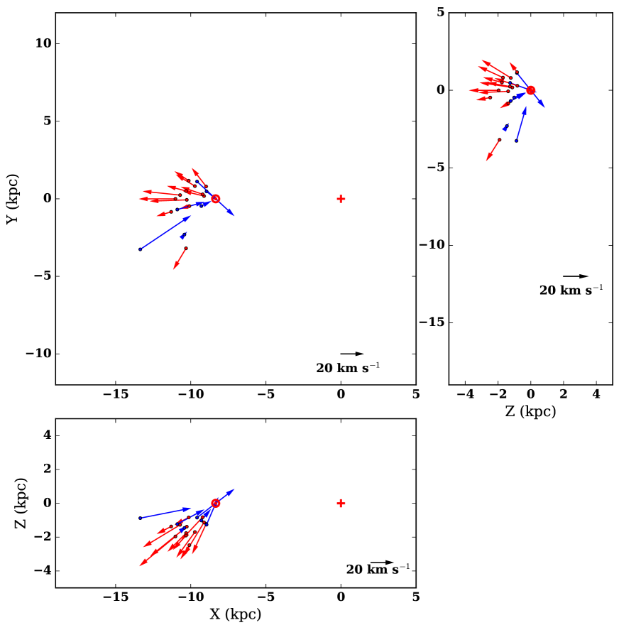
Figure 11: 2D Projection of $V_{\rm obs}$-$V_{\rm model}$ in Galactocentric Cartesian coordinate for group B, with $R>$ 9 kpc, -2.0 $<Z<$ $-$0.8 kpc. $V_{\rm model}$ was calculated by using $\Theta+\overline{V_{s}}$ = 180  km s^-1.

In the lower panel of Fig. 9, the -2.0 $<Z<$ $-$0.8 kpc group has the highest S and very low $\Theta$+$\overline{V_{s}}$, and $\overline{W_{s}}$. Further inspection of the value of $V_{\rm obs}$-$V_{\rm model}$ confirms the systematic peculiar motion of this group as shown in Fig. 11. For further discussion, we denote this group as group B.

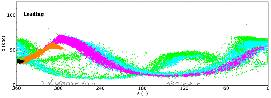
Figure 12: Position-distance diagrams of the Leading arm of the Sgr stellar stream. Color dots are HM10 Leading arm model (Figure 7 of Law & Majewski (2010a)). Open circles are groups A and B offplane sources listed in Table 6.

In Table 6, we list the detailed source information of these two groups. Both groups are made up of off-plane sources. Radial velocities of stars within the northern group (group A) can be modelled by stars with a rotational speed $\Theta$+$\overline{V_{s}}$ = 189$\pm$9  km s^-1, with peculiar motion $\overline{U_{s}}$ = 12$\pm$8  km s^-1, $\overline{W_{s}}$ = 33$\pm$6  km s^-1 away from the Galactic plane. Radial velocities of stars within the southern group (group B) can be modeled by stars with rotational speed $\Theta$+$\overline{V_{s}}$ = 176$\pm$13  km s^-1, with peculiar motion $\overline{U_{s}}$ = 25$\pm$9  km s^-1, and $\overline{W_{s}}$ = $-$54$\pm$11  km s^-1 away from the Galactic plane. Regarding their Sgr stellar stream coordinates (columns 7 and 8 of Table 6), they seem to be aligned with the orbital plane of the Sgr stellar stream. For a comparison with the Sgr stellar stream, in Fig. 12, we overlay these moving group sources on a longitude-distance diagram of the L1/L2 wrap of LM10 model. These off-plane sources are within 5 kpc of the Sun.

In the LM10 model, the Sgr stream is not expected to be located within 13 kpc of the Sun, while in the model of Majewski (2004), the intersection between L2 wrap of the Sgr stellar stream and the Galactic plane is very close to the Sun. It should be mentioned that in the LM10 model, all Leading arm SDSS Constrains are beyond 18 kpc (Table 1 of Law & Majewski, 2010b). This can be due to method bias, as the majority of halo stream features are identified by stellar overdensity, which can be overlooked at nearest distances due to severe disc contaminations. Although observational constraints of stream features at near distances are rare, Kundu et al. (2002) found eight giant stars with kinematics, abundances and locations roughly consistent with leading tidal arm of the Sagittarius arm. 6 out of these 8 giant stars are within 5 kpc of the Sun. Even for LM10 model, they did not exclude the possibility of the existence of Sgr stream stars in nearby ($D<$10 kpc) region (see discussions in Section 8.2 of Law & Majewski, 2010b). Taking into account of the Galactic location and kinematics of groups A and B sources, they may be thick disc stars with their kinematics affected by the halo stellar stream or very old Sgr stream debris. Future measurements of proper motions and determinations of the full 3D motions and Galactic orbits of these sources will be crucial for testing these scenarios.

In the lower panel of Fig. 9, there exist two “high" peculiar motion groups, groups 1 and 2 in Fig. 9, one is the 0.3 $<Z<$ 0.5 kpc group and the other is the -0.8 $<Z<$ $-$0.5 kpc group. Further investigation of the values of $V_{\rm obs}$-$V_{\rm model}$ of these two groups reveals most of sources within these groups are actually normal disc stars, the large peculiar motion seen in Fig. 9 are due to two very high speed sources, which were listed in Table 7. With same method, another high speed source was identified in the -1.4 $<Z<$ $-$0.8 kpc, 5 $<R<$ 9 kpc group, which was also listed in Table 7. In Figure 9, groups including these high speed sources are highlighted with red labels 1, 2 and 3.

In the upper panels of Fig. 9, another outlier is the -0.1 $<Z<$ 0.1 kpc group (group D), with the largest value of $S$ and a relatively high rotation speed of 237 $\pm$ 7  km s^-1 compared to other groups. The large S of this group is due to inclusion of a large number of objects from extended regions. For comparison, in the lower panel, for the 9 $<R<$ 13 kpc, -0.1 $<Z<$ 0.1 kpc group, the value of S is only $\sim$25.0  km s^-1. Un-modeled peculiar motions due to non-axisymmetric perturbations from spiral arms and/or the bar could explain the large value of S in group D.

In Fig. 9, we noticed dependences of the rotational speed and the velocity dispersion on the Galactic plane distance. In the 1st lower left panel of Fig. 9, it can be seen that the velocity dispersion S increases with $Z$. In the second column of Fig. 9: in the group of $Z>$ 0, 5 $<R<$ 9 kpc, and group of $Z<$ 0, $R>$ 9 kpc, there is a clear trend that rotational speed decreases with $Z$. These phenomena are consistent with stellar dynamics theory: old thick disc stars which are dynamically evolved sources tend to have slower rotational speeds and higher velocity dispersions.

In the 0.3 $<Z<$ 0.8 kpc, $R>9$ kpc region, which we denote as group C, there can be seen an increasing of $\Theta$+$\overline{V_{s}}$. Such an enhancement in rotation speed is hard to explain by the stellar dynamics mentioned above. Fig. 13 illustrates $V_{\rm obs}$-$V_{\rm model}$ for the sources in this group. In the Figure, one can see outward and upward bulk motions for many sources. Considering the locations of these sources, it is possible that they trace peculiar motions or flows associated with the Perseus spiral arm. Kirsanova et al. (2017) found that high-mass star forming regions (HMSFRs) in the Perseus arm traced by 6.7 GHz methanol masers between $85^{\circ}<l<124^{\circ}$, and $173^{\circ}<l<196^{\circ}$ are moving outward and rotate about the Galaxy at a higher velocity with respect to the gas tracers (CO and CS). As can be seen in Figure 7 of Kirsanova et al. (2017), the kinematics of these HMSFRs are somewhat simiar to our group C SiO masers, which supports our viewpoint that there exist large scale peculiar motions in the Perseus arm.

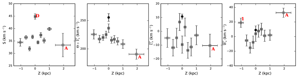
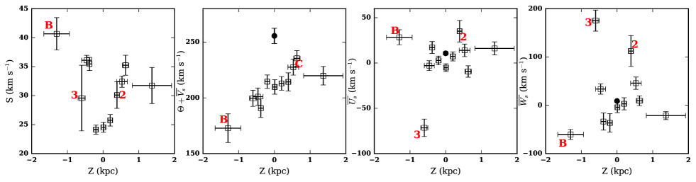
Figure 9: Visualization of best estimated $S$, $\Theta+\overline{V_{s}}$, $\overline{U_{s}}$, $\overline{W_{s}}$ of each spatially binned subsamples.Upper panels are $R$-$Z$ binned groups of 5 $<R<$ 9 kpc, lower panels are $R$-$Z$ binned groups of $R>$ 9 kpc. Red colour A, B, C and 1, 2, 3 denote three moving groups and 3 high speed sources. The filled circle denotes Solar motions where (U_⊙, V_⊙,W_⊙) = (10.7$\pm$1.8, 15.6$\pm$6.8, 8.9$\pm$0.9)  km s^-1(Reid et al., 2014). Horizonal “errorbars” denote the min($Z$) and max($Z$) of stars in the binned range of $Z$; vertical errorbars denote 1$\sigma$ uncertainties of $S$, $\Theta+\overline{V_{s}}$, $\overline{U_{s}}$, $\overline{W_{s}}$.

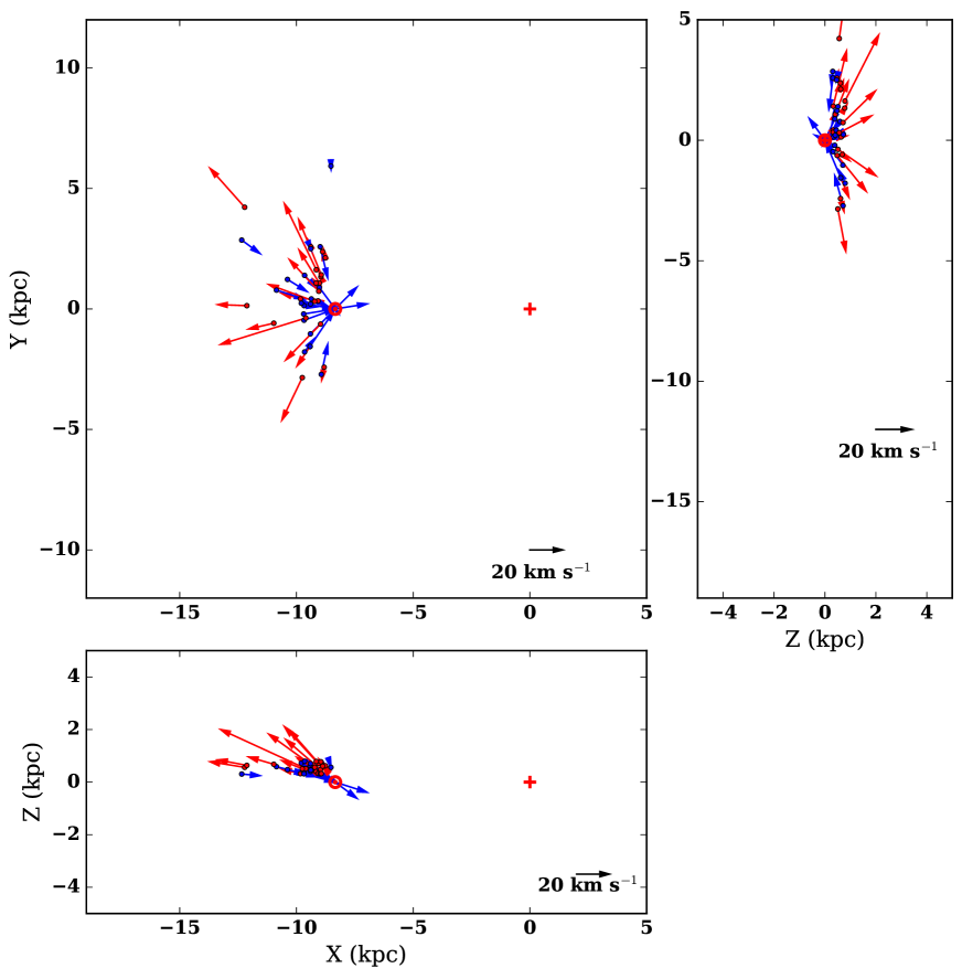
Figure 13: 2D Projection of $V_{\rm obs}$-$V_{\rm model}$ in Galactocentric Cartesian coordinate for group C, with $R>$ 9 kpc, 0.3 $<Z<$ 0.8 kpc. $V_{\rm model}$ was calculated by adopting $\Theta+\overline{V_{s}}$ = 220  km s^-1.

In order to evaluate whether the systematic motions identified in groups A, B and C were statistically significant, we made simulations to test the null hypothesis that the systematic peculiar motions are not true but within statistical errors. In the simulation, we generate "trial" stars with identical Galactic coordinates. Distance errors were simulated by varying the nominal distance values up to 20% as a 1 $\sigma$ error. For kinematics, we assume they follow the kinematic model of disc stars, with rotational speed, $\Theta$, varying as function of Galactic plane distances ranging from 225  km s^-1 to 180  km s^-1, plus normal random motions ($\overline{U_{s}}$, $\overline{V_{s}}$, $\overline{W_{s}}$) with 1$\sigma$ errors ranging from 25  km s^-1 to 40  km s^-1. Then (S, $\overline{U_{s}}$, $\Theta$+$\overline{V_{s}}$, $\overline{W_{s}}$) were estimated by the same procedure as applied to the observational data.

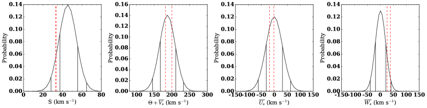
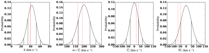
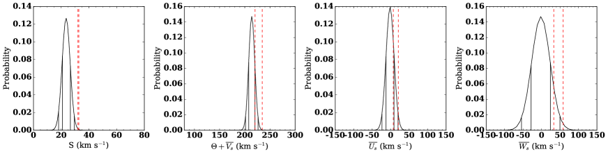
Figure 17: Probability distributions for (S, $\overline{U_{s}}$, $\Theta$+$\overline{V_{s}}$, $\overline{W_{s}}$) estimated via simulation for null hypothesis testing. Top, middle and bottom panels are results of group A, B and C, respectively. Solid black lines denote 1$\sigma$ (68%) and 2$\sigma$ (95%) boundaries of simulations. Red dashed lines denote 1$\sigma$ range of (S, $\overline{U_{s}}$, $\Theta$+$\overline{V_{s}}$, $\overline{W_{s}}$) estimated using real data.

We conducted 1000 trials, and then calculated the probability distributions of (S, $\overline{U_{s}}$, $\Theta$+$\overline{V_{s}}$, $\overline{W_{s}}$), which are shown in Figure 17. In Fig. 17, black vertical lines denote 1$\sigma$ (68%) and 2$\sigma$ (95%) boundaries of the simulations, red dashed lines denote the 1$\sigma$ range of (S, $\overline{U_{s}}$, $\Theta$+$\overline{V_{s}}$, $\overline{W_{s}}$) estimated with real data. Top, middle and bottom panels are results of the groups A, B and C respectively. For all three groups, the value of $\overline{W_{s}}$ estimated by real data were within 1$\sigma$ to 2$\sigma$ range of simulations. Thus, statistically, we were $\sim$70% confident that the systematic peculiar motions vertical to the Galactic plane of all three groups are real. Especially, for the group C, the disagreement between simulations and real data is significant for all the four (S, $\overline{U_{s}}$, $\Theta$+$\overline{V_{s}}$, $\overline{W_{s}}$) parameters. Future measurements of proper motions and determinations of full 3D motions and Galactic orbits of these sources will be crucial for better understanding these bulk motions.

5 Summary

We conducted an SiO maser survey towards 221 O-rich AGBs projected on the Sgr stellar stream region. In total, we detected maser emission in 44 AGBs, of which 35 were new detections. We found that the WISE colour-colour diagram method provides an effective way to select O-rich Miras for SiO maser survey.

We compiled a Galactic SiO maser catalogue that includes $\sim$2300 sources. We then cross matched this maser catalogue with the GCVS and AAVSO variable catalogues and the 2MASS and WISE point souces catalogues and calculated the PLR distance and WISE luminosity distances for $\sim$1000 sources. By studying the Galactic distribution of sources, we determined a typical height scale (0.40 kpc) of disc SiO masers, and identified 42 off-plane SiO masers. 50% of these off-plane SiO masers were discovered in this work.

We identified three very high speed stars and found systematic peculiar motions in three groups (70% confidence) by comparing the radial velocities with models of disc stars. The most statistically significant group is within the thick disc, with 0.3 $<Z<$ 0.8 kpc, $R>9$ kpc, which might be tracing an outward (13$\pm$7  km s^-1) and upward (44$\pm$14  km s^-1) flow in the Perseus arm. The other two moving groups are mainly made up of off-plane sources. The northern group can be modeled by disc stars with rotational speed $\sim$190  km s^-1, and peculiar motion $\overline{W_{s}}$ = 34$\pm$6  km s^-1 away from the Galactic plane; the southern group can be modeled by disc stars with rotational speed $\sim$180  km s^-1, and peculiar motion of $\overline{U_{s}}$ = 25$\pm$9  km s^-1, $\overline{W_{s}}$ = $-$54$\pm$11  km s^-1 away from the Galactic plane. As these two off-plane groups are aligned with the Sgr orbital plane, we suspect that they could be thick disc stars whose kinematics might be affected by the halo stellar stream or very old stream debris. Future measurements of proper motions and determinations of full 3D motions and Galactic orbits of these sources will be crucial to confirm/deny our conclusions.

For disc SiO maser sources, model fitting on radial velocities allows us to reveal dependences of the rotational speed and the velocity dispersion on the distances from the Galactic plane, i.e., stars with higher Galactic plane distances tend to have large velocity dispersion and rotate slowly within the Galactic disc. These trends are consistent with the theory of stellar dynamics. With $\Theta_{0}$= 240  km s^-1, we derived a velocity lag of 15  km s^-1 and 55  km s^-1 for disc and off-plane SiO maser sources respectively.

Appendix A Distance estimate

Distances is the key parameter to study the Galactic distribution. For Miras with known period, their distances can be calculated based on the period luminosity relation (PLR). For AGB stars without period or Ks magnitude but with the WISE colour available, we derived WISE luminosity distances by using an empirical formula calibrated with O-rich Miras, in which the distance is function of the $W4$ magnitude and a dereddened colour [$W1$^′-$W4$]. Formulas used to derive the PLR distances and WISE luminosity distances are given in the section A.1 and A.2 respectively. .

A.1 PLR Distance

First we collect K_s magnitudes from 2MASS catalogue (Cutri et al., 2003) and periods from the General Catalog of Variable Stars (GCVS, Samus’ et al. (2003)) and/or International Variable Star Index Catalog (AAVSO, Watson (2006)). Then the absolute K magnitudes of O-rich Miras were derived by using the infrared (K) period-luminosity relation formula (from Whitelock et al., 2008) of

$$M_{K}=-3.51[\log~{}P-2.38]-7.25.$$ (4)

Comarison between the observed and absolute magnitudes gives the initial estimation of distance without interstellar extinction taking into account.

$$D=10^{(m_{Ks}-M_{K}+5)/5}$$ (5)

With this distance, the interstellar extinction (A_V) is estimated using the three-dimensional Galactic extinction model (Drimmel et al., 2003). The extinction A_V is solved by using the FORTRAN script Av3$\_$FEB03.f given by Drimmel, Cabrera-Lavers, & López-Corredoira (2003). The $A_{V}$ is converted to $A_{Ks}$ by

$$A_{Ks}=R(Ks)\times E(B-V)=A_{V}\frac{R(Ks)}{R(V)}$$ (6)

where $R(V)$ = 3.10 and $R(Ks)$ = 0.306 are the V and Ks band extinction coefficients from Fitzpatrick (1999); Yuan et al. (2013). The $A_{Ks}$ is then used to estimate the dereddened magnitude,

$$m^{\prime}_{Ks}=m_{Ks}-A_{Ks},$$ (7)

and recalculate the distance. Two iterations usually suffice.

A.2 WISE Luminosity Distance

According to the WISE Explanatory Supplement documentation of All-Sky Data Release that bright sources will saturate WISE detector . The saturation limits are 8.1, 6.7, 3.8, and -0.4 mag in the $W1$-$W4$ bands, respectively (green lines in Fig. 14). For saturated objects, WISE fits the PSF to the unsaturated pixels on the images to recover the saturated pixels and yield photometry for these objects (we call this PSF-fit photometry). The bright source photometry limits for the WISE 4 bands are 2, 1.5, $-$3, and $-$4 mag (red lines in Fig. 14). When they are brighter than this limit, all the pixels are saturated and no unsaturated pixels are available to fit to the PSF. As can be seen in Fig. 14, $\sim$ 100 bright nearby AGBs are totally saturated. In WISE 1, 2 and 3 band, photometry are PSF-fit photometry for most of our targets. $W4$ band is the best band in which the saturation is not so serious. In addition, for sources within $\sim$2 kpc, although they are not totally saturated, their PSF-fit photometry tend to be underestimated, which result in a overestimate of distance.

Regarding the interstellar extinctions, we consider the method in Section A.1 that makes use of the 3D extinction model to correct for $W1$ band interstellar extinction.

$$A_{W1}=R(W1)\times E(B-V)=A_{V}\frac{R(W1)}{R(A)},$$ (8)

where $R(V)$ = 3.10 and $R(W1)$ = 0.18 are the $V$ band and WISE $W1$ band extinction coefficients from Fitzpatrick (1999) and Yuan et al. (2013). Then we correct $W1^{\prime}$ with the extinction A_W1,

$$W1^{\prime}=W1-A_{W1}$$ (9)

The $W4$ band luminosity,

$$L_{W4}=L_{\star}+L_{dust}=\alpha\times L_{\star}$$ (10)

where, L_dust is the W4 band luminosity from the dusty envelope, and L_⋆ is the inherent W4 band luminosity of the star, $\alpha$ is a reddening factor. Here we tried to correct a de-reddening $W4$ band magnitude to let

$$W4C=\beta\times(W1^{\prime}-W4)+\gamma\times W4\propto\log(L_{\star}\times D^{-2})$$ (11)

where $\beta$ and $\gamma$ are constants.

If we further assume that L_⋆ is a constant, then the formula 11 can be written as

$$\log~{}D=\textit{a}\times W4+\textit{b}\times(W1^{\prime}-W4)+\textit{c}.$$ (12)

We use the Markov chain Monte Carlo (MCMC) method to fit a, b and c by minimizing the differences between the model distance, $D_{WISE}$ and the PLR distance, $D_{PLR}$. In Fig. 15, we present histogram of the MCMC model fitting results, with the best fitted model, a = 0.200, b = 0.306, c = -0.663, indicated by red lines. In the bottom right panel of Fig. 15, shown is histogram of $D_{WISE}$-$D_{PLR}$. For the best fitted model, the mean, median and standard deviation of $D_{WISE}$-$D_{PLR}$ is $-$0.26, 0.03 and 1.52 kpc. It can be seen that $D_{WISE}$-$D_{PLR}$ is within 2 kpc for most of sources. Most of the outliers are sources towards the Bulge and Galactic centre region, where the extinction are usually very large ($A_{Ks}$ $>$ 2). Their deviation can also be seen in lower left panel of Fig. 5, i.e., sources with $D_{WISE}$ $\sim$ 8 to 15 kpc, but with $D_{PLR}$ from 10 kpc to more than 25 kpc. The discrepancy may also be attributed to underestimates of the extinction estimated by three-dimensional Galactic extinction model (Drimmel et al., 2003) .

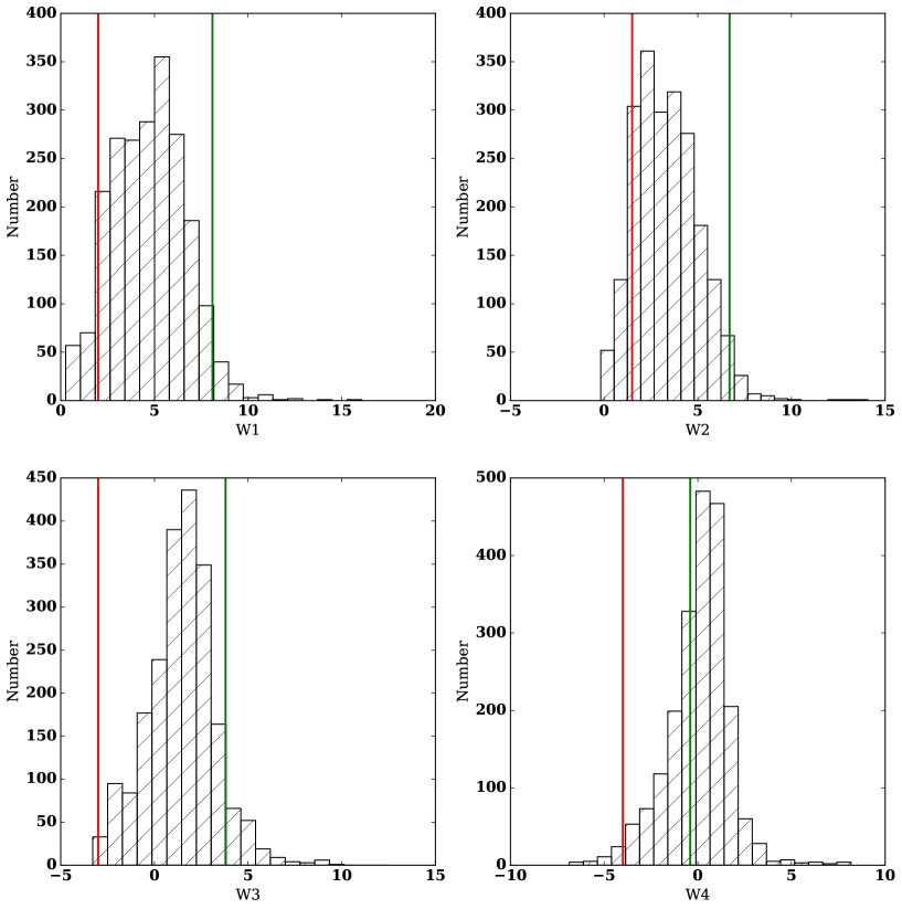
Figure 14: Histogram of WISE magnitudes of $W1$ , $W2$, $W3$ and $W4$, respectively. Green vertical lines denote the saturation limits for the WISE 4 bands that are 8.1, 6.7, 3.8, and -0.4 mag, respectively. Red vertical lines denote the bright source photometry limits for the WISE 4 bands that are 2, 1.5, $-$3, and $-$4 mag, respectively.

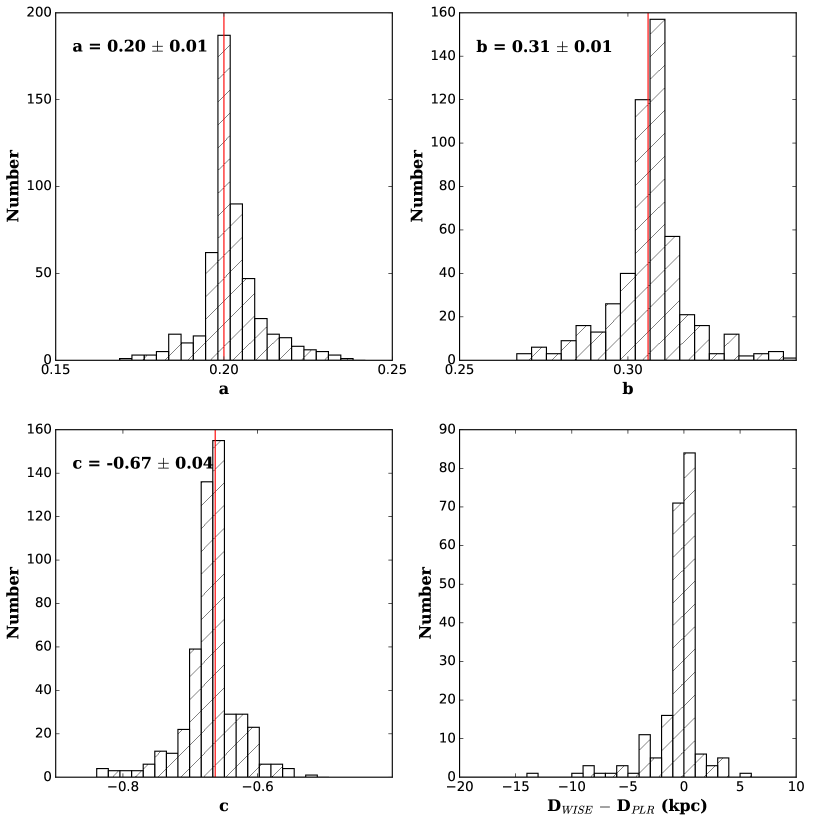
Figure 15: Top left panel is the histogram of $a$ in Equation 12 estimated with the MCMC method. The best estimated values and uncertainties are label in the top left corner. Top right panel and bottom left panel is same as the top left panel but for the constant $b$ and $c$ in Equation 12. Red vertical lines denote the best estimate values. bottom right panel is the histogram for differences between $D_{WISE}$ and $D_{PLR}$.

Table 8: List of observed Sources

Source	R.A.(J2000)	DEC.(J2000)	Other	Star	Spectral	$V^{\ast}$	Period	Maser
Name	(h:m:s)	(d:m:s)	Name	Type	Type	(km s-1)	(days)	Detection
G000.760$+$51.066	15 00 12.98	$+$03 15 41.7		*	M5	…		NN
G001.856$+$72.531	13 53 55.19	$+$17 16 50.1	XZ Boo	LPV*	M5	…		NN
G003.378$+$47.338	15 16 02.72	$+$02 10 04.6	Z Ser	sr*	M5	-25.00		NN
G003.602$+$43.085	15 29 38.03	$-$00 23 45.8	AM Ser	sr*	M2	…		NN
G003.848$+$44.341	15 26 10.68	$+$00 31 56.5	V380 Ser	sr*	Me	…		NN
G004.482$+$32.104	16 05 46.29	$-$06 42 27.8	BD Oph	Mi*	M6e	-432.72		YY
G006.077$+$30.607	16 13 53.44	$-$06 32 16.4	V2577 Oph	Mi*	…	…		NN
G008.104$+$45.840	15 28 43.67	$+$03 49 43.6	MW Ser	Mi*	M8	…		YY
G010.937$+$35.609	16 07 08.16	$-$00 18 53.6	AI Ser	Mi*	…	…		NN
G011.025$+$53.268	15 08 25.77	$+$09 36 18.4	FV Boo	Mi?	M9III	…		YY
G011.131$+$37.023	16 02 49.18	$+$00 36 40.6	DW Ser	Mi*	M1e	…		NN
G011.159$-$41.196	21 04 36.85	$-$33 16 47.3	X Mic	Mi*	M…	19.0		YY
G012.097$+$32.492	16 19 37.28	$-$01 15 47.2	CM Ser	Mi*	…	-36.93	220.6	NN
G012.230$-$32.998	20 27 29.17	$-$30 48 37.3	V5556 Sgr	Mi*	M8	…		NN
G012.444$+$38.278	16 00 58.08	$+$02 10 27.9	BC Ser	Mi*	M5e	49		NN
G012.901$-$63.916	22 53 30.71	$-$32 55 39.9	SS PsA	Mi*	…	…		NN
G014.428$+$52.730	15 14 41.21	$+$11 03 31.6		*	…	…		NN
G015.405$-$35.139	20 40 02.99	$-$28 47 31.2	R Mic	Mi*	M4e	10.00		YN
G016.257$+$64.629	14 33 28.30	$+$17 36 46.9	CO Boo	Mi*	…	…	280.0	NN
G016.831$-$45.308	21 26 44.10	$-$29 51 04.7	S Mic	Mi*	M3-5.5e	49		NN
G017.647$-$37.951	20 54 26.42	$-$27 44 15.9	RX Mic	Mi*	…	-51.01		NN
G017.863$+$72.316	14 04 52.15	$+$21 21 19.1		*	…	…		NN
G019.002$-$39.495	21 02 20.78	$-$27 05 14.9	RR Cap	Mi*	M6e:	-63		YY
G019.408$+$42.783	15 56 29.69	$+$09 01 50.2	RU Ser	Mi*	…	11.0	282.2	NN
G019.509$-$56.308	22 18 00.24	$-$29 36 13.8	R PsA	Mi*	M6+e	-25.0		NN
G020.708$-$31.502	20 30 06.77	$-$23 30 41.5	AY Cap	sr*	…	46.55		NN
G021.290$-$47.410	21 38 41.87	$-$27 12 34.1	RV PsA	Mi*	…	-24.36		NN
G021.343$-$32.293	20 34 07.64	$-$23 14 58.6	AK Cap	LPV*	M4III	…		NN
G021.513$-$53.023	22 03 45.83	$-$28 03 04.2	S PsA	Mi*	M3e	-92.0		YN
G022.158$+$40.858	16 07 17.66	$+$09 55 52.5	U Ser	Mi*	M4-6e	-31.00		YY
G022.461$+$33.819	16 32 55.55	$+$06 51 29.7	SS Her	Mi*	M0-5+e	-46.0		NN
G022.943$-$31.448	20 32 34.16	$-$21 41 26.5	RU Cap	Mi*	M9	-3		YY
G023.139$-$38.703	21 02 42.82	$-$23 46 54.8	CE Cap	sr*	…	…		NN
G023.291$-$34.188	20 44 09.74	$-$22 18 12.9	CC Cap	sr*	M6.5	…		NN
G023.376$-$39.816	21 07 36.63	$-$23 55 13.4	V Cap	Mi*	M5.5-6e	-36.0		YY
G023.664$+$40.100	16 12 09.44	$+$10 36 26.1	DN Her	Mi*	M6.5	-46.0		NN
G025.952$-$42.117	21 19 37.45	$-$22 42 26.9	CH Cap	sr*	…	…		NN
G026.343$-$35.418	20 52 39.24	$-$20 20 00.3	BX Cap	LPV*	…	…		NN
G026.645$-$39.261	21 08 33.06	$-$21 20 51.5	X Cap	Mi*	M2e…	-37.55		NN
G028.805$-$31.578	20 40 32.08	$-$17 03 28.2	TX Cap	Mi*	M4	9.0		NN
G032.106$-$32.402	20 48 08.58	$-$14 47 01.0	U Cap	Mi*	M5.5e	…	203.8	NN
G032.852$-$33.566	20 53 35.02	$-$14 39 50.4	XX Cap	LPV*	M5	-15.68		NN
G033.078$-$37.937	21 10 37.52	$-$16 10 24.8	Z Cap	Mi*	M2e:	-64		NN
G033.245$-$56.048	22 23 12.94	$-$22 03 25.5	RT Aqr	Mi*	M5	-34.00		NN
G033.519$-$53.484	22 12 50.93	$-$21 09 51.9	AQ Aqr	Mi*	…	-90.68		NN
G035.634$-$40.082	21 22 00.82	$-$15 09 33.1	T Cap	Mi*	M6e:	42.00		NN
G036.242$-$55.590	22 23 30.38	$-$20 18 49.2	KU Aqr	LPV*	M3III	…		NN
G037.206$-$55.581	22 24 13.46	$-$19 47 42.7	AV Aqr	Mi*	M	-73.0		NN
G037.250$-$44.253	21 39 53.43	$-$15 40 35.4	CK Cap	LP?	…	…		NN
G038.070$+$66.469	14 37 11.58	$+$26 44 11.7	R Boo	Mi*	M4-8e	-58.00		YY
G038.666$-$42.354	21 34 22.91	$-$13 58 29.3	Y Cap	Mi*	M8.5	…		NN
G039.040$-$42.707	21 36 10.46	$-$13 52 04.9	UU Cap	sr*	M3/4III	-4.08		NN
G041.021$+$62.253	14 56 41.05	$+$27 30 25.2	NP Boo	Mi*	…	…		NN
G041.037$-$51.361	22 11 13.36	$-$16 07 47.2	YY Aqr	sr*	…	…		NN
G041.058$-$50.181	22 06 44.98	$-$15 38 40.3	BM Aqr	sr*	M3(III)	-21.00		NN
G041.181$-$31.735	20 59 00.66	$-$07 32 29.4	VV Aqr	Mi*	…	-183.18	140.7	NN
G041.307$-$63.037	22 57 06.46	$-$20 20 35.7	S Aqr	Mi*	M6e	-58		NN
G041.346$-$64.747	23 04 00.56	$-$20 54 24.0	MN Aqr	Mi*	M7:	…		NN
G045.006$-$52.540	22 19 54.43	$-$14 24 07.0	SS Aqr	Mi*	M2	2		NN
G045.032$-$36.798	21 23 03.67	$-$07 06 29.4	RZ Aqr	Mi*	M9	…		NN
Column 1 are Galactic coordinate notated source names; column 2 and 3 are equatorial coordinates; column 4 are Bayer
designation names of variables; column 5 and 6 are stellar and Spectral types; column 7 are radial velocities,
column 8 are periods; column 9 denote detections for v=1 and 2 SiO J=1-0 maser lines.

Table 9: continued

List of observed Sources Source R.A.(J2000) DEC.(J2000) Other Star Spectral $V^{\ast}$ Period Maser Name (h:m:s) (d:m:s) Name Type Type (km s^-1) (days) Detection G045.734$-$38.770 21 31 06.50 $-$07 34 20.4 HY Aqr Mi* M8 -20 YN G051.533$-$62.801 23 04 17.19 $-$16 00 35.9 EQ Aqr sr* M3/4 … NN G051.533$-$62.801 23 04 17.19 $-$16 00 35.9 EQ Aqr sr* M3/4 … NN G051.594$-$50.205 22 19 35.29 $-$09 40 32.6 ZZ Aqr sr* … … NN G055.342$-$64.356 23 13 24.09 $-$15 19 16.0 UX Aqr Mi* M4e … NN G058.824$+$57.868 15 17 14.71 $+$36 21 33.4 RT Boo Mi* M6.5e 35.00 NN G060.246$-$57.280 22 54 55.48 $-$09 22 27.7 TT Aqr sr* M3III … NN G064.549$+$76.014 13 48 44.69 $+$33 43 34.2 RT CVn Mi* M5e: -12 YN G069.300$-$72.233 23 52 14.54 $-$15 51 17.2 Z Aqr sr* M1/2Ib/II 68.90 NN G070.786$-$60.449 23 18 58.18 $-$07 18 50.9 DM Aqr Mi* … … NN G073.394$-$77.357 00 10 57.96 $-$18 34 23.4 AC Cet LPV* M3III -12.90 NN G077.779$-$73.062 00 02 07.39 $-$14 40 33.1 W Cet S* S5.5-7/1.5 13.0 NN G083.632$-$79.140 00 22 30.89 $-$18 32 45.2 LPV* M … 201.3 NN G085.581$-$67.859 23 57 54.07 $-$08 57 31.2 V Cet Mi* M3/5(III)e 51 YN G093.803$-$63.776 00 01 38.63 $-$03 45 23.3 DU Psc sr* … -14.09 NN G094.565$-$80.456 00 32 21.61 $-$18 39 08.5 ET Cet sr* M6 … NN G096.925$+$58.455 14 22 52.92 $+$53 48 37.3 S Boo Mi* M5-6e -17.00 NN G120.894$-$64.174 00 47 53.14 $-$01 18 58.7 SX Cet sr* … … NN G131.720$-$64.091 01 06 45.20 $-$01 28 51.8 Z Cet Mi* M5-6e 3 YN G133.797$-$53.388 01 17 34.56 $+$08 55 52.0 S Psc Mi* M5+-7e 14.6 YN G134.760$-$49.278 01 22 58.48 $+$12 52 04.0 U Psc Mi* M4e -35.0 NN G135.687$-$52.241 01 22 59.11 $+$09 50 50.2 * … … NN G141.402$+$31.072 08 03 59.72 $+$73 24 30.6 SW Cam Mi* M5e … NN G141.940$-$58.536 01 30 38.35 $+$02 52 52.5 R Psc Mi* M4-8e -45 YN G144.537$-$70.053 01 20 37.11 $-$08 24 52.6 CU Cet sr* M2 … NN G146.496$-$59.340 01 38 30.12 $+$01 21 40.1 SW Cet LPV* M5 … NN G146.657$-$43.306 02 02 28.33 $+$16 16 11.2 RY Ari LPV* M6 … NN G147.548$-$60.663 01 38 32.50 $-$00 03 43.6 LPV* … … 168.8 NN G149.396$-$46.550 02 04 37.67 $+$12 31 36.9 S Ari Mi* M4-5e -27.0 NY G150.794$-$47.560 02 06 27.29 $+$11 12 46.1 * M0 … NN G152.650$-$53.296 02 00 42.61 $+$05 31 53.7 TT Psc sr* M4 … NN G153.782$-$52.608 02 04 24.28 $+$05 50 17.1 * … … NN G156.088$-$52.393 02 09 46.83 $+$05 21 41.7 * M2 … NN G156.914$-$37.397 02 42 46.87 $+$18 01 13.4 * … … NN G158.558$-$71.111 01 35 47.92 $-$11 22 30.2 FY Cet sr* M3/4III … NN G158.741$-$40.144 02 41 44.10 $+$14 56 12.3 * … … NN G159.484$-$38.173 02 48 12.39 $+$16 16 28.3 BD Ari sr* M7 … NN G159.820$-$47.007 02 29 17.65 $+$08 44 08.4 * … … NN G160.874$-$49.439 02 26 18.94 $+$06 18 52.5 * M4 … NN G162.261$-$42.711 02 44 51.63 $+$11 20 05.7 * … … NN G162.904$-$49.384 02 30 49.91 $+$05 36 58.3 * … … NN G163.265$-$46.216 02 39 00.42 $+$08 03 41.2 * M4.5 … NN G165.494$-$43.684 02 50 14.10 $+$09 09 16.2 * … … NN G165.616$-$40.899 02 57 27.52 $+$11 18 05.3 YZ Ari Mi* M8 25 433.4 YY G166.965$-$54.751 02 26 02.31 $-$00 10 42.0 R Cet Mi* M4-5e 42.00 YN G168.980$+$37.738 08 40 49.50 $+$50 08 11.9 X UMa Mi* M4e -83 YY G173.516$-$38.103 03 23 35.71 $+$09 23 55.0 * M6.5 … NN G175.479$+$46.580 09 30 56.58 $+$44 41 01.7 * M6 25.80 NN G175.507$+$50.992 09 55 19.92 $+$44 00 29.5 YZ UMa LPV* M5V: … NN G175.651$-$77.193 01 34 25.98 $-$18 58 28.2 AP Cet sr* M7 … NN G176.154$-$30.578 03 51 44.23 $+$13 06 28.8 * M6.5 … NN G177.272$-$37.906 03 32 32.90 $+$07 25 32.2 * M5.5 … NN G177.576$-$33.940 03 44 59.43 $+$09 56 36.0 CH Tau sr* M1 … NN G179.335$+$42.704 09 08 47.86 $+$42 09 21.6 DH Lyn sr* M7 … NN G179.379$+$30.743 08 05 03.70 $+$40 59 08.1 IR … … YY G179.553$-$33.716 03 50 06.63 $+$08 52 09.0 * M7.5 … NN G180.069$-$36.185 03 43 43.89 $+$06 55 30.5 V1083 Tau Mi* M9 82 YY G180.829$+$32.784 08 16 46.88 $+$40 07 53.3 W Lyn Mi* M6 … YY G181.209$-$73.392 01 50 33.86 $-$17 39 00.9 DH Cet sr* M5 … NN G181.889$-$44.366 03 22 31.61 $+$00 31 48.0 * M5.5 … NN G182.006$-$35.653 03 49 27.68 $+$06 04 40.4 V1191 Tau Mi* M8.5 … YY G182.059$-$45.211 03 20 15.56 $-$00 06 29.0 * M0 … NN G183.100$+$30.845 08 08 50.31 $+$37 52 20.6 * … … NN G183.385$+$34.661 08 28 08.04 $+$38 20 23.0 RX Lyn sr* M … NN

Table 10: continued

List of observed Sources Source R.A.(J2000) DEC.(J2000) Other Star Spectral $V^{\ast}$ Period Maser Name (h:m:s) (d:m:s) Name Type Type (km s^-1) (days) Detection G183.614$+$31.966 08 14 50.64 $+$37 40 11.7 RT Lyn Mi* M6e … NY G184.565$-$83.387 01 16 52.83 $-$23 50 40.1 RT Cet LPV* M2 … NN G184.714$+$33.826 08 24 55.36 $+$37 06 53.1 AGB* M7 … NN G185.796$+$37.989 08 46 12.58 $+$36 54 42.8 * … … NN G185.814$+$62.448 10 48 34.26 $+$36 17 35.2 * M8 … NN G186.761$+$33.619 08 25 31.37 $+$35 24 13.9 X Lyn Mi* M5 7.0 NN G187.196$+$36.638 08 40 25.60 $+$35 36 23.7 AGB* M … NN G188.099$+$48.741 09 40 15.16 $+$36 06 19.0 Z LMi LPV* M … NN G188.152$+$51.648 09 54 38.71 $+$36 05 22.8 U LMi sr* M6 -32 NN G188.344$+$50.247 09 47 42.79 $+$35 58 15.1 * … … NN G188.664$-$39.190 03 51 15.85 $-$00 15 53.8 V* M7 … NN G189.897$-$30.567 04 21 45.82 $+$03 53 50.1 * M7.5 … NN G190.865$+$51.122 09 52 09.00 $+$34 23 29.3 * … … NN G190.894$+$48.491 09 39 25.61 $+$34 14 53.0 VZ LMi Mi* M … 292.2 NN G195.025$-$53.735 03 11 53.14 $-$11 52 32.4 SS Eri Mi* M5… 48 YY G196.576$+$45.020 09 25 17.07 $+$29 58 47.6 TW Leo LPV* Me … 216.4 NN G197.990$+$33.262 08 34 28.05 $+$26 13 47.2 * … … NN G198.081$+$74.222 11 40 43.82 $+$30 03 17.0 AY UMa LPV* M3 … NN G198.593$-$69.596 02 16 00.08 $-$20 31 10.5 RY Cet Mi* M6+e: 16.0 YY G203.330$+$30.788 08 30 22.54 $+$21 09 27.4 * M… … NN G203.660$+$52.559 10 02 41.02 $+$26 41 36.0 SV Leo Mi* M7 … NN G204.101$+$32.634 08 38 46.63 $+$21 09 32.7 UV Cnc LPV* M0 … NN G204.907$+$32.225 08 38 06.76 $+$20 22 50.2 DK Cnc sr* M3 … NN G206.317$+$31.191 08 35 46.31 $+$18 53 44.7 U Cnc Mi* M2e 72 NN G206.346$+$47.275 09 41 34.11 $+$23 50 33.9 * … … NN G211.919$+$50.661 10 00 01.99 $+$21 15 43.9 V Leo Mi* M5-6e -23.00 YY G212.108$+$46.532 09 43 25.67 $+$19 51 40.0 RS Leo Mi* M5e … NN G212.164$+$57.683 10 29 21.56 $+$23 03 44.9 UY Leo LPV* M7III: … NN G212.195$+$63.282 10 53 09.43 $+$24 21 31.1 RU Leo LPV* M3 … NN G214.232$+$43.058 09 31 51.13 $+$17 15 05.5 LPV* … … 177.7 NN G217.372$+$50.948 10 05 58.80 $+$18 06 04.9 V* M8 … NN G218.786$+$51.178 10 08 14.78 $+$17 21 30.6 DD Leo sr* M8 … NN G220.968$+$59.976 10 44 40.35 $+$19 25 23.8 EW Leo sr* M5 … NN G223.002$+$48.943 10 04 15.94 $+$13 58 57.7 RY Leo sr* M2 22.00 NN G234.525$+$52.514 10 31 27.87 $+$09 21 07.0 * M7 … NN G235.246$+$67.258 11 23 40.03 $+$16 51 07.0 TZ Leo Mi* M8 18.0 YY G236.412$+$81.845 12 18 46.68 $+$23 38 43.2 AB Com Mi* M … 195.6 NN G238.855$+$56.995 10 52 11.04 $+$09 48 55.2 * … … NN G239.757$+$46.896 10 20 50.19 $+$03 21 09.0 SZ Sex Mi* … … 147.9 NN G243.022$+$46.682 10 25 43.90 $+$01 28 08.7 SY Sex Mi* … … 208.7 NN G248.071$-$84.665 01 11 36.38 $-$30 06 29.4 U Scl Mi* M5e -8 YY G250.569$+$57.710 11 10 50.78 $+$05 27 34.7 S Leo Mi* M6:e 106 NN G254.436$+$65.121 11 36 54.77 $+$09 31 45.9 ZZ Leo sr* M0 … NN G261.694$+$46.256 11 01 55.14 $-$07 39 41.8 RT Crt Mi* M8 41.00 YY G262.094$+$61.213 11 37 48.11 $+$04 19 24.8 IW Vir LPV* M5 … NN G264.438$+$71.690 12 05 14.81 $+$12 21 37.9 SU Vir Mi* M2-5.5e 19 NN G264.623$+$48.097 11 12 45.30 $-$07 17 54.5 U Crt Mi* M0e … NN G268.755$+$80.079 12 27 57.87 $+$18 48 08.5 TV Com LPV* M2 … NN G276.361$+$63.050 12 04 36.16 $+$02 37 10.6 TZ Vir sr* M5 … NN G283.439$+$80.931 12 38 43.06 $+$18 32 41.7 DO Com sr* … … NN G283.995$+$74.423 12 30 58.11 $+$12 18 30.6 CV Vir Mi* … … 148.4 NN G289.779$+$69.653 12 33 08.38 $+$07 15 00.3 CI Vir LPV* M6 … NN G289.879$+$76.356 12 38 51.52 $+$13 48 13.9 KM Com LPV* M2 23.7 NN G294.615$+$58.166 12 33 52.99 $-$04 25 19.6 Y Vir Mi* M5.5e: 9 NN G309.119$+$49.507 13 07 55.40 $-$13 09 58.9 RV Vir Mi* A5 33 NN G311.686$+$77.932 12 58 59.74 $+$15 11 21.7 RX Com Mi* … … 210.5 NN G312.284$+$53.849 13 13 41.63 $-$08 37 05.7 HH Vir sr* … … NN G315.566$+$57.522 13 18 30.52 $-$04 41 03.2 VY Vir Mi* M3pev … YY G320.482$+$58.454 13 27 48.13 $-$03 10 22.9 V Vir Mi* M5-6e 33 NN G325.570$+$85.690 12 58 38.90 $+$23 08 21.0 T Com Mi* M2 15.0 YY G326.771$+$45.772 13 58 59.11 $-$13 56 59.1 * M6 … NN G330.757$+$45.262 14 10 22.10 $-$13 18 11.8 Z Vir Mi* M5e 68 YN

Table 11: continued

List of observed Sources Source R.A.(J2000) DEC.(J2000) Other Star Spectral $V^{\ast}$ Period Maser Name (h:m:s) (d:m:s) Name Type Type (km s^-1) (days) Detection G331.573+49.548 14 04 53.44 $-$09 11 41.2 RR Vir Mi* … -43.0 215.7 NN G331.781+33.351 14 35 49.00 $-$23 36 29.4 LX Lib Mi* … -10.60 NN G332.578+54.382 13 58 37.59 $-$04 34 32.8 SY Vir Mi* M6 … NN G333.388+33.799 14 39 59.87 $-$22 34 26.2 EP Lib Mi* … … NN G334.109+36.043 14 37 29.14 $-$20 19 41.2 LY Lib Mi* … … YY G335.504+35.524 14 42 46.26 $-$20 12 36.1 SX Lib Mi* M6e… … YY G335.646+44.462 14 24 29.54 $-$12 25 07.3 V* M1III … NN G335.670+35.438 14 43 27.21 $-$20 12 53.3 GS Lib Mi* M6 … NN G336.386+35.873 14 44 36.98 $-$19 32 28.2 TW Lib Mi* … 81.94 NN G336.532+38.006 14 40 22.18 $-$17 39 26.9 V Lib Mi* M5e 15 YN G337.373+32.451 14 55 21.62 $-$22 00 19.6 EG Lib Mi* M5 5 YY G337.755+51.213 14 15 44.47 $-$05 52 06.4 CF Vir Mi* M5e 44.03 NN G339.224+44.663 14 32 59.87 $-$10 56 03.2 KS Lib Mi* Me … YY G339.938+43.686 14 36 54.68 $-$11 28 40.8 * M6.5 … NN G340.371+66.478 13 48 08.49 $+$07 49 13.2 HX Boo sr* M5 … NN G340.829+31.460 15 08 10.66 $-$21 10 00.3 YY Lib Mi* Me … YN G342.142+33.667 15 06 26.19 $-$18 43 56.2 RT Lib Mi* M2.5-5.5e 41.0 NN G342.197+32.029 15 10 44.36 $-$20 01 08.4 T Lib Mi* M4 -48 NN G344.240+30.203 15 21 23.96 $-$20 23 18.5 S Lib Mi* M1.5-4e 294.0 NN G345.104+35.879 15 08 54.49 $-$15 29 51.0 TT Lib Mi* M3e -47.27 NN G346.039+45.775 14 46 18.42 $-$07 15 49.9 AQ Vir Mi* M5e -4.0 NN G346.087+47.560 14 42 00.64 $-$05 49 57.2 XY Vir Mi* … 29.89 154.8 NN G348.715+50.518 14 39 59.19 $-$02 26 48.6 * … … NN G349.797+58.296 14 21 51.90 $+$03 54 27.8 AO Vir Mi* M4 … NN G350.237+30.144 15 38 05.25 $-$17 01 54.2 EK Lib sr* M7e … NN G350.511+84.894 13 07 53.22 $+$23 37 28.6 * … … NN G350.719+30.733 15 37 39.75 $-$16 19 02.8 IRC-20290 IR M7 … NN G350.868+30.821 15 37 48.00 $-$16 09 57.1 W Lib Mi* … 22.0 NN G351.579+32.192 15 35 41.95 $-$14 45 16.3 * … … NN G352.221+57.421 14 28 03.54 $+$04 06 33.3 * … … NN G353.548+50.630 14 48 52.46 $-$00 19 37.0 * M7 … NN G353.826+42.588 15 11 41.26 $-$06 00 41.2 Y Lib Mi* M5.5e -7.00 YN G356.016+48.746 14 58 42.58 $-$00 33 16.5 * M6 … NN G356.642+59.618 14 28 30.27 $+$07 17 37.1 AP Vir Mi? M3 … YY G358.057+46.657 15 08 32.60 $-$01 00 45.2 * M6 … NN G358.765+67.787 14 06 29.61 $+$13 29 05.5 Z Boo Mi* M6e 40 NN

Table 12: Observational results of SiO masers.

	SiO v=1 J=1-0 maser line				SiO v=2 J=1-0 maser line
Source	VLSR	T${}^{\ast}_{A}$(peak)	Int. Flux	rms	VLSR	T${}^{\ast}_{A}$(peak)	Int. Flux	rms	Ref.
Name	(K km s-1)	(K)	(K km s-1)	(K)	(K km s-1)	(K)	(K km s-1)	(K)
G004.482$+$32.104	$-$8.8	0.18	0.79	0.03	$-$10.8	0.10	0.14	0.02	2
G008.104$+$45.840	41.0	0.37	1.39	0.05	42.8	0.16	0.72	0.04	3
G011.025$+$53.268	4.5	1.61	11.76	0.08	$-$13.7	0.54	2.36	0.07	4
G011.159$-$41.196	17.8	0.72	1.64	0.09	18.2	0.28	0.94	0.05	1
G015.405$-$35.139	19.9	0.20	0.87	0.04	—	—	—	0.04	1
G019.002$-$39.495	$-$51.8	0.94	5.27	0.07	$-$51.3	0.40	1.52	0.07	1
G019.509$-$56.308	$-$29.0	1.26	3.76	0.07	$-$29.7	0.36	1.10	0.06	1
G021.513$-$53.023	$-$100.8	0.22	0.53	0.04	—	—	—	0.04	1
G022.158$+$40.858	$-$15.0	0.69	1.34	0.11	$-$15.6	1.01	1.41	0.10	1
G022.943$-$31.448	9.8	1.33	4.30	0.12	7.0	1.38	2.65	0.11	4
G023.376$-$39.816	$-$20.9	1.41	2.33	0.06	$-$16.5	0.25	0.88	0.05	1
G038.070$+$66.469	$-$42.4	0.53	2.69	0.06	$-$44.0	0.22	0.87	0.04	3
G045.734$-$38.770	26.3	0.23	0.47	0.03	—	—	—	0.03	1
G064.549$+$76.014	26.3	0.11	0.27	0.03	26.3	0.15	0.54	0.02	1
G085.581$-$67.859	50.9	0.22	1.09	0.04	—	—	—	0.04	1
G131.720$-$64.091	4.0	0.29	0.94	0.04	—	—	—	0.04	1
G133.797$-$53.388	4.3	1.10	5.68	0.10	4.3	1.48	4.23	0.11	1
G141.940$-$58.536	$-$57.0	0.82	2.01	0.09	$-$56.8	0.58	1.38	0.09	5
G149.396$-$46.550	—	—	—	0.05	9.5	0.16	0.75	0.05	1
G165.616$-$40.899	13.0	0.88	1.59	0.07	12.5	0.52	0.71	0.07	6
G166.965$-$54.751	35.2	0.38	0.90	0.05	—	—	—	0.05	7
G168.980$+$37.738	$-$82.9	0.38	0.65	0.06	$-$83.5	0.20	0.26	0.04	1
G179.379$+$30.743	$-$10.6	0.81	2.59	0.08	$-$9.2	0.72	2.01	0.07	2
G180.069$-$36.185	58.0	0.09	0.25	0.02	57.4	0.11	0.29	0.02	1
G180.829$+$32.784	$-$24.8	0.41	0.40	0.08	$-$25.1	0.54	0.62	0.07	1
G182.006$-$35.653	61.0	0.11	0.47	0.02	61.3	0.19	0.85	0.03	1
G183.614$+$31.966	—	—	—	0.03	27.5	0.13	0.32	0.02	1
G195.025$-$53.735	33.2	0.27	0.42	0.04	35.3	0.12	0.37	0.03	1
G198.593$-$69.596	$-$2.8	0.55	1.41	0.06	$-$3.4	0.19	0.62	0.04	1
G211.919$+$50.661	$-$25.5	1.23	4.30	0.09	$-$24.2	0.57	2.03	0.07	3
G235.246$+$67.258	12.9	0.30	0.59	0.04	12.7	0.35	0.39	0.04	1
G248.071$-$84.665	$-$10.3	0.32	1.03	0.06	$-$10.4	0.35	0.89	0.05	1
G261.694$+$46.256	32.9	0.38	1.10	0.05	32.8	0.28	0.55	0.05	1
G315.566$+$57.522	72.0	0.11	0.72	0.03	70.7	0.23	0.83	0.04	1
G325.570$+$85.690	26.1	2.01	5.22	0.09	25.2	2.66	8.13	0.09	3
G330.757$+$45.262	66.8	0.21	0.39	0.03	—	—	—	0.03	1
G334.109$+$36.043	$-$25.4	0.23	1.14	0.05	$-$25.3	0.27	0.24	0.05	1
G335.504$+$35.524	$-$31.2	0.83	3.08	0.08	$-$31.0	0.56	2.02	0.07	1
G336.532$+$38.006	18.1	0.22	0.28	0.03	—	—	—	0.03	1
G337.373$+$32.451	$-$7.8	1.42	4.64	0.13	$-$9.6	0.47	0.99	0.08	2
G339.224$+$44.663	70.7	0.18	0.93	0.04	69.9	0.14	0.64	0.03	2
G340.829$+$31.460	$-$3.9	0.15	0.48	0.03	—	—	—	0.03	1
G353.826$+$42.588	14.9	0.14	0.48	0.03	—	—	—	0.03	2,3
G356.642$+$59.618	37.2	0.34	0.41	0.04	37.0	0.44	0.60	0.04	1
Note: column 1 are source name; columns 2, 3, 4, 5 and columns 6, 7, 8, 9 are $V_{\rm LSR}$, peak antennas temperatures (in unit of K),
integrated flux density (in unit of K km s-1), and 1$\sigma$ rms of spectra for v=1 and v=2 SiO maser lines. Column 9 denote references.
Reference: (1) this paper; (2) Ita et al. (2001); (3) Kim et al. (2010); (4) Kim et al. (2010); (5) Cho & Kim (2012); (6) Deguchi et al. (2012);
(7) Indermuehle & McIntosh (2014)

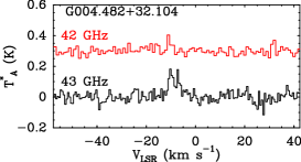
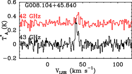
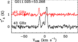
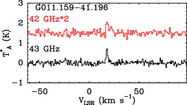
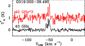
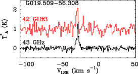
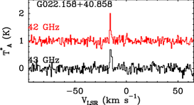
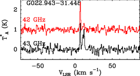
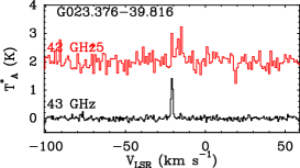
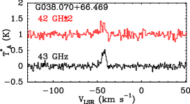
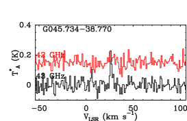
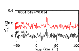
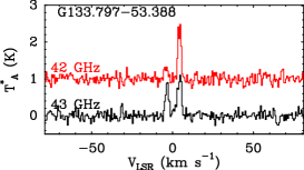
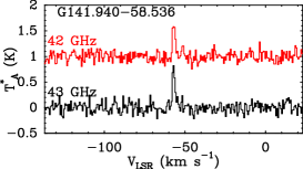
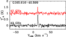
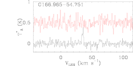
Figure 16: SiO maser spectra. In case both v=1 and v=2 masers are detected, the v=2 (42 GHz) maser lines are denoted by red histograms. Some low flux density 42 GHz maser lines are scaled up, with the scale factors labeled in the plot.

Fig. 16 continue

References

- Belokurov et al. (2014) Belokurov, V., Koposov, S. E., Evans, N. W., et al. 2014, MNRAS, 437, 116
- Belokurov et al. (2006) Belokurov, V., Zucker, D. B., Evans, N. W., et al. 2006, ApJ, 642, L137
- Benson et al. (1990) Benson, P. J., Little-Marenin, I. R., Woods, T. C., et al. 1990, ApJS, 74, 911
- Bland-Hawthorn & Gerhard (2016) Bland-Hawthorn, J. & Gerhard, O. 2016, ARA&A, 54, 529
- Carrell et al. (2012) Carrell, K., Wilhelm, R., & Chen, Y. 2012, AJ, 144, 18
- Cho & Kim (2012) Cho, S.-H. & Kim, J. 2012, AJ, 144, 129
- Correnti et al. (2010) Correnti, M., Bellazzini, M., Ibata, R. A., Ferraro, F. R., & Varghese, A. 2010, ApJ, 721, 329
- Cutri & et al. (2012) Cutri, R. M. & et al. 2012, VizieR Online Data Catalog, 2311
- Cutri et al. (2003) Cutri, R. M., Skrutskie, M. F., van Dyk, S., et al. 2003, 2MASS All Sky Catalog of point sources.
- Deguchi (2007) Deguchi, S. 2007, in IAU Symposium, Vol. 242, Astrophysical Masers and their Environments, ed. J. M. Chapman & W. A. Baan, 200–207
- Deguchi et al. (2004) Deguchi, S., Fujii, T., Glass, I. S., et al. 2004, PASJ, 56, 765
- Deguchi et al. (2007) Deguchi, S., Fujii, T., Ita, Y., et al. 2007, PASJ, 59, 559
- Deguchi et al. (2012) Deguchi, S., Sakamoto, T., & Hasegawa, T. 2012, PASJ, 64, 4
- Deguchi et al. (2010) Deguchi, S., Shimoikura, T., & Koike, K. 2010, PASJ, 62, 525
- Dehnen & Binney (1998) Dehnen, W. & Binney, J. J. 1998, MNRAS, 298, 387
- Demers & Battinelli (2007) Demers, S. & Battinelli, P. 2007, A&A, 473, 143
- Drake et al. (2013) Drake, A. J., Catelan, M., Djorgovski, S. G., et al. 2013, ApJ, 765, 154
- Drimmel et al. (2003) Drimmel, R., Cabrera-Lavers, A., & López-Corredoira, M. 2003, A&A, 409, 205
- Fitzpatrick (1999) Fitzpatrick, E. L. 1999, PASP, 111, 63
- Haikala et al. (1994) Haikala, L. K., Nyman, L.-A., & Forsstroem, V. 1994, A&AS, 103
- Hall et al. (1990) Hall, P. J., Allen, D. A., Troup, E. R., Wark, R. M., & Wright, A. E. 1990, MNRAS, 243, 480
- Helou & Walker (1988) Helou, G. & Walker, D. W., eds. 1988, Infrared astronomical satellite (IRAS) catalogs and atlases. Volume 7: The small scale structure catalog, Vol. 7, 1–265
- Honma et al. (2012) Honma, M., Nagayama, T., Ando, K., et al. 2012, PASJ, 64
- Huxor & Grebel (2015) Huxor, A. P. & Grebel, E. K. 2015, MNRAS, 453, 2653
- Ibata et al. (2001) Ibata, R., Lewis, G. F., Irwin, M., Totten, E., & Quinn, T. 2001, ApJ, 551, 294
- Indermuehle & McIntosh (2014) Indermuehle, B. T. & McIntosh, G. C. 2014, MNRAS, 441, 3226
- Ishihara et al. (2010) Ishihara, D., Onaka, T., Kataza, H., et al. 2010, A&A, 514, A1
- Ita et al. (2001) Ita, Y., Deguchi, S., Fujii, T., et al. 2001, A&A, 376, 112
- Izumiura et al. (1995) Izumiura, H., Catchpole, R., Deguchi, S., et al. 1995, ApJS, 98, 271
- Izumiura et al. (1998) Izumiura, H., Deguchi, S., & Fujii, T. 1998, ApJ, 494, L89
- Izumiura et al. (1994) Izumiura, H., Deguchi, S., Hashimoto, O., et al. 1994, ApJ, 437, 419
- Jiang et al. (1995) Jiang, B. W., Deguchi, S., Izumiura, H., Nakada, Y., & Yamamura, I. 1995, PASJ, 47, 815
- Kim et al. (2010) Kim, J., Cho, S.-H., Oh, C. S., & Byun, D.-Y. 2010, ApJS, 188, 209
- Kirsanova et al. (2017) Kirsanova, M. S., Sobolev, A. M., & Thomasson, M. 2017, ArXiv:1705.02197
- Koposov et al. (2012) Koposov, S. E., Belokurov, V., Evans, N. W., et al. 2012, ApJ, 750, 80
- Kundu et al. (2002) Kundu, A., Majewski, S. R., Rhee, J., et al. 2002, ApJ, 576, L125
- Kwon & Suh (2012) Kwon, Y.-J. & Suh, K.-W. 2012, Journal of Korean Astronomical Society, 45, 139
- Law & Majewski (2010a) Law, D. R. & Majewski, S. R. 2010a, ApJ, 718, 1128
- Law & Majewski (2010b) Law, D. R. & Majewski, S. R. 2010b, ApJ, 714, 229
- Li et al. (2010) Li, J., An, T., Shen, Z.-Q., & Miyazaki, A. 2010, ApJ, 720, L56
- Lian et al. (2014) Lian, J., Zhu, Q., Kong, X., & He, J. 2014, A&A, 564, A84
- Little-Marenin & Little (1990) Little-Marenin, I. R. & Little, S. J. 1990, AJ, 99, 1173
- Lynden-Bell & Lynden-Bell (1995) Lynden-Bell, D. & Lynden-Bell, R. M. 1995, MNRAS, 275, 429
- Majewski (2004) Majewski, S. R. 2004, Publ. Astron. Soc. Australia, 21, 197
- Majewski et al. (2003) Majewski, S. R., Skrutskie, M. F., Weinberg, M. D., & Ostheimer, J. C. 2003, ApJ, 599, 1082
- Matsunaga et al. (2005) Matsunaga, N., Deguchi, S., Ita, Y., Tanabe, T., & Nakada, Y. 2005, PASJ, 57, L1
- McMillan & Binney (2010) McMillan, P. J. & Binney, J. J. 2010, MNRAS, 402, 934
- Nakashima et al. (2000) Nakashima, J.-i., Jiang, B. W., Deguchi, S., Sadakane, K., & Nakada, Y. 2000, PASJ, 52, 275
- Nikutta et al. (2014) Nikutta, R., Hunt-Walker, N., Nenkova, M., Ivezić, Ž., & Elitzur, M. 2014, MNRAS, 442, 3361
- Pasetto et al. (2012) Pasetto, S., Grebel, E. K., Zwitter, T., et al. 2012, A&A, 547, A70
- Reid et al. (2014) Reid, M. J., Menten, K. M., Brunthaler, A., et al. 2014, ApJ, 783, 130
- Ruhland et al. (2011) Ruhland, C., Bell, E. F., Rix, H.-W., & Xue, X.-X. 2011, ApJ, 731, 119
- Samus’ et al. (2003) Samus’, N. N., Goranskii, V. P., Durlevich, O. V., et al. 2003, Astronomy Letters, 29, 468
- Shi et al. (2012) Shi, W. B., Chen, Y. Q., Carrell, K., & Zhao, G. 2012, ApJ, 751, 130
- Shiki & Deguchi (1997) Shiki, S. & Deguchi, S. 1997, ApJ, 478, 206
- Sjouwerman et al. (2002) Sjouwerman, L. O., Lindqvist, M., van Langevelde, H. J., & Diamond, P. J. 2002, A&A, 391, 967
- Slater et al. (2013) Slater, C. T., Bell, E. F., Schlafly, E. F., et al. 2013, ApJ, 762, 6
- Suh & Kwon (2009) Suh, K.-W. & Kwon, Y.-J. 2009, Journal of Korean Astronomical Society, 42, 81
- Suh & Kwon (2011) Suh, K.-W. & Kwon, Y.-J. 2011, MNRAS, 417, 3047
- Tian et al. (2015) Tian, H.-J., Liu, C., Carlin, J. L., et al. 2015, ApJ, 809, 145
- van der Veen & Habing (1988) van der Veen, W. E. C. J. & Habing, H. J. 1988, A&A, 194, 125
- Vivas & Zinn (2006) Vivas, A. K. & Zinn, R. 2006, AJ, 132, 714
- Watson (2006) Watson, C. L. 2006, Society for Astronomical Sciences Annual Symposium, 25, 47
- Whitelock et al. (2008) Whitelock, P. A., Feast, M. W., & van Leeuwen, F. 2008, MNRAS, 386, 313
- Wright et al. (2010) Wright, E. L., Eisenhardt, P. R. M., Mainzer, A. K., et al. 2010, AJ, 140, 1868
- Xin & Zheng (2013) Xin, X.-S. & Zheng, X.-W. 2013, Research in Astronomy and Astrophysics, 13, 849
- Yuan et al. (2013) Yuan, H. B., Liu, X. W., & Xiang, M. S. 2013, MNRAS, 430, 2188