Dense scale selection over space, time and space-time

Abstract

Scale selection methods based on local extrema over scale of scale-normalized derivatives have been primarily developed to be applied sparsely — at image points where the magnitude of a scale-normalized differential expression additionally assumes local extrema over the domain where the data are defined. This paper presents a methodology for performing dense scale selection, so that hypotheses about local characteristic scales in images, temporal signals and video can be computed at every image point and every time moment. A critical problem when designing mechanisms for dense scale selection is that the scale at which scale-normalized differential entities assume local extrema over scale can be strongly dependent on the local order of the locally dominant differential structure. To address this problem, we propose a methodology where local extrema over scale are detected of a quasi quadrature measure involving scale-space derivatives up to order two and propose two independent mechanisms to reduce the phase dependency of the local scale estimates by: (i) introducing a second layer of post-smoothing prior to the detection of local extrema over scale and (ii) performing local phase compensation based on a model of the phase dependency of the local scale estimates depending on the relative strengths between first- vs. second-order differential structure. This general methodology is applied over three types of domains: (i) spatial images, (ii) temporal signals and (iii) spatio-temporal video. Experiments demonstrate that the proposed methodology leads to intuitively reasonable results with local scale estimates that reflect variations in the characteristic scales of locally dominant structures over space and time.

65D18, 65D19, 68U10

1 Introduction

The notion of scale is essential when computing features from image data for purposes in biological or artificial visual perception. Results from biological research regarding the early visual areas in the LGN and V1 (Hubel and Wiesel [19, 20, 21]; DeAngelis et al. [12, 11]) as well as theoretical results from normative theory of visual operations (Lindeberg [39, 43]) based on scale-space theory (Iijima [22]; Witkin [67]; Koenderink [26, 27]; Koenderink and van Doorn [28, 30]; Lindeberg [33, 38]; Florack [14]; Sporring et al. [59]; Weickert et al. [66]; ter Haar Romeny et al. [62, 61]) state that local image measurements in terms of receptive fields constitute a both natural and efficient model for expressing early visual operations.

When applying such spatial or spatio-temporal receptive fields at multiple spatial and temporal scales, a basic observation that one can make is that the responses that are obtained from the receptive field operators can be strongly dependent on the scale levels at which they are applied. Thus, one may raise the problem whether it is possible from the data itself to generate hypotheses about local appropriate scales in the image data, so as to adapt subsequent processing to the local image structures. Initially, this problem could possibly be seen as intractable. Would it at all be possible to generate hypotheses about interest scale levels before recognizing the objects we are interested in or defining the specific purpose for which the scale estimates are to be used? Research in (Lindeberg [33, 35, 34]) with follow-up work by several authors (Bretzner et al. [5, 4]; Chomat et al. [8]; Lowe [49]; Mikolajczyk and Schmid [51]; Lazebnik et al. [31]; Rothganger et al. [56]; Bay et al. [2]; Tuytelaars and Mikolajczyk [64]; Negre et al. [52]; Lindeberg [40, 42]) has, however, demonstrated that such an approach is feasible (see [37, 41] for overviews). A general framework for automatic selection of local characteristic scales can be formulated based on the detection of local extrema over scale of scale-normalized feature responses. Specifically, such scale estimates transform in a scale-covariant way under spatial scaling transformations of the image domain, which is a highly desirable property of a scale selection mechanism, since it implies that the scale estimates will automatically follow local scale variations in the image data. Corresponding local scale selection mechanisms can also be expressed over temporal and spatio-temporal domains (Lindeberg [46, 44, 45]).

A common property of most of the successful applications of scale selection to computer vision applications, however, is that the scale selection method is applied sparsely over the image domain, most commonly at interest points. If attempting to perform dense scale selection based on the two most common rotationally invariant differential invariants for interest point detection, the spatial Laplacian or the determinant of the spatial Hessian, then the results of scale selection will usually not be stable or useful far away from the interest points.

To address this problem, an initial mechanism for dense scale selection was proposed in (Lindeberg [35]) based on a the detection of local extrema over scale of a spatial quasi quadrature measure that constitutes a rotationally invariant measure of the amount of energy in the first- and second-order differential structure of a spatial image. Modifications of this approach were used by Almansa and Lindeberg [1] for estimating the local scale of fingerprint patterns for fingerprint recognition and were specifically shown to improve the quality of minutiae extraction. Related methods for scale selection have been developed by Kadir and Brady [24] and Sporring et al. [58]) by detecting peaks of weighted entropy measures or Lyaponov functionals over scale, by minimizing normalized error measures over scale (Lindeberg [36]), by determining local scales for variable bandwidth mean shift from the scale bandwidth that maximizes the norm of the normalized mean shift vector (Comaniciu et al. [10]), by detecting maxima of steered energy responses over scales (Ng and Bharath [53]), by comparing reliability measures from statistical classifiers for texture analysis at multiple scales (Kang et al. [25]), by measuring the size variations of the regions that pixels belong to under total variation (TV) flow (Brox and Weickert [6]), by measuring local oscillations in signals (Jones and Le [23]) or by computing image segmentations from the scales at which a supervised classifier delivers class labels with the highest reliability measure (Loog et al. [48]; Li et al. [32]). Specifically, a more algorithmic way of generating scale estimates for image matching away from the locations of interest points was recently proposed by Hassner et al. [18] and Tau and Hassner [60] by considering subspaces generated by local image descriptors computed over multiple scales to improve the performance of stereo matching.

Closely related issues of estimating dominant scales in signals have been studied in wavelet theory and local frequency analysis (Cohen [9]). For example, a local Gaussian-weighted windowed Fourier transform of a 1-D signal corresponds to filtering with Gabor functions [15]. Mallat and Hwang [50] proposed to characterize singularities in terms of Lipshitz exponents and detected maxima in the wavelet transform. Pure wavelet and/or local frequency based methods have, however, been less developed for 2-D image data or 2+1-D video data.

The subject of this article is to perform a deeper study into the problem of dense scale selection for images and video. A basic problem that can be observed if performing dense scale selection based on the basic quasi quadrature measure in [35] is that the local scale estimates can be strongly phase dependent. If applied to a sine wave in one or two dimensions, the scale estimates can be biased depending on the relative strength of first-order vs. second-order differential structure. To reduce this phase dependency, we will consider two independent mechanisms in terms of (i) spatial smoothing and (ii) local phase compensation. We will specifically analyze the properties of these mechanisms, determine free parameters in the corresponding methods and show that these mechanisms may reduce the local phase dependency substantially. We will also generalize this dense scale selection mechanism to the spatio-temporal domain, to perform simultaneous dense scale selection of both local spatial and temporal scales. Compared to wavelet-based approaches for local frequency analysis, the methods that we propose are invariant to rotations over the spatial domain. Additionally, we prove that both the spatial and the temporal scale estimates are provably covariant under independent scaling transformations of the spatial and the temporal domains, implying that the local scale estimates are guaranteed to automatically follow local variations in the spatial extent and the temporal duration of spatial, temporal or spatio-temporal image structures, which is a highly desirable property of a scale selection mechanism. Experiments on different types of spatial images, temporal signals and spatio-temporal video demonstrate that the proposed theory leads to dense spatial and temporal scale maps with intuitively reasonable properties.

2 Dense spatial scale selection over a purely spatial domain

The context we consider is a spatial scale-space representation $L(x,y;\;s)$ defined from any 2-D image $f(x,y)$ by convolution with Gaussian kernels

(1) $$g(x,y;\;s)=\frac{1}{2\pi s}e^{-(x^{2}+y^{2})/2s}$$

at different spatial scales $s$ (Iijima [22]; Witkin [67]; Koenderink [26]; Koenderink and van Doorn [28, 30]; Lindeberg [33, 38]; Florack [14]; Sporring et al. [59]; Weickert et al. [66]; ter Haar Romeny [61])

(2) $$L(\cdot,\cdot;\;s)=g(\cdot,\cdot;\;s)*f(\cdot,\cdot)$$

and with $\gamma$-normalized derivatives defined at any scale $s$ according to (Lindeberg [35])

(3) $$\partial_{\xi}=s^{\gamma_{s}/2}\,\partial_{x},\quad\partial_{\eta}=s^{\gamma_{s}/2}\,\partial_{y}.$$

If attempting to perform dense local scale selection in the possibly most straightforward manner, by detecting local extrema of the scale-normalized Laplacian $\nabla_{norm}^{2}L=s\,(L_{xx}+L_{yy})$ or the scale-normalized determinant of the Hessian $\det{\cal H}_{norm}L=s^{2}\,(L_{xx}L_{yy}-L_{xy}^{2})$ at points that are not interest points, one will soon find out that the resulting scale estimates will be strongly dependent on the points at which they are computed. The reason for this is that the underlying interest point detectors primarily respond to very specific aspects of the second-order differential structure, see Figure 1 for an illustration. Scale selection by the scale-normalized Laplacian or the scale-normalized determinant of the Hessian operators is therefore primarily intended for image structures that lead to strong responses for these differential operators, such as spatial interest points (Lindeberg [35, 40, 42]).

original image	$|\nabla^{2}L|$	$\sqrt{|\det{\cal H}L|}$	$\sqrt{{\cal Q}_{(x,y),1}L}$	$\sqrt{{\cal Q}_{(x,y),2}L}$	$\sqrt{{\cal Q}_{(x,y)}L}$
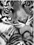
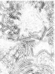
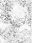
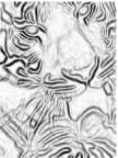
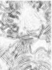
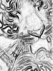
	$|\overline{\nabla^{2}}L|$	$\sqrt{|\overline{\det{\cal H}}L|}$	$\sqrt{\overline{\cal Q}_{(x,y),1}L}$	$\sqrt{\overline{\cal Q}_{(x,y),2}L}$	$\sqrt{\overline{\cal Q}_{(x,y)}L}$

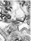
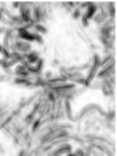
Figure 1: The result of computing (top row) the unsmoothed quasi quadrature measure ${\cal Q}_{(x,y),norm}L$ and (bottom row) the post-smoothed quasi quadrature entity $\overline{\cal Q}_{(x,y),norm}L$ with their underlying first- and second-order components at scale $t=16$ for $C_{s}=1/\sqrt{2}$. For comparison, (top row) Laplacian and determinant of the Hessian responses as well as (bottom row) the result of applying spatial smoothing to these differential operators for relative post-smoothing scale $c=1$ are also shown at the same scale to illustrate how Laplacian and determinant of the Hessian responses will be limited to specific aspects of local image structures and thereby the limitations of using the Laplacian or the determinant of the Hessian operators only for dense scale selection. (Image size: $480\times 640$.)

For the performing dense scale selection, it is therefore more natural to seek a differential expression that responds to wider classes of image structures, comprising both first- and second-order differential structures, and without bias towards primarily specific aspects of the second-order differential image structure.

2.1 A spatial quasi quadrature measure

By combining the rotationally invariant differential invariants (i) the gradient magnitude

(4) $$|\nabla L|^{2}=L_{x}^{2}+L_{y}^{2}$$

as a measure of the amount of first-order structure and (ii) the Frobenius norm of the Hessian matrix

(5) $$\|{\cal H}L\|_{F}^{2}=L_{xx}^{2}+2L_{xy}^{2}+L_{yy}^{2}$$

as a measure of the amount of second-order structure, we will consider extensions of the following quasi quadrature measure (Lindeberg [35, Eq. (63)])

(6) $$\begin{split}{\cal Q}_{(x,y),norm}L&=s\,(L_{x}^{2}+L_{y}^{2})+C_{s}\,s^{2}\,(L_{xx}^{2}+2L_{xy}^{2}+L_{yy}^{2})\end{split}$$

based on scale-normalized derivatives for $\gamma_{s}=1$. This differential entity can be seen as an approximation of the notion of a quadrature pair of an odd and even filter (Gabor [15]) as more traditionally formulated based on a Hilbert transform (Bracewell [3, p. 267-272]) and then extended to 2-D image space, while being confined within the family of differential expressions based on Gaussian derivatives and additionally being rotationally invariant.

If complemented by spatial integration, the components of this quasi quadrature measure are specifically related to the following class of energy measures over the frequency domain (Lindeberg [35, App. A.3]) (here expressed in terms of multi-index notation for the partial derivatives $x^{\alpha}=x_{1}^{\alpha_{1}}\dots x_{D}^{\alpha_{D}}$ with $|\alpha|=\alpha_{1}+\dots+\alpha_{D}$):

(7) $$E_{m,\gamma-norm}=\int_{x\in{\mathbb{R}}^{D}}\sum_{|\alpha|=m}s^{m\gamma_{s}}\,L_{x^{\alpha}}^{2}\,dx=\frac{s^{m\gamma_{s}}}{(2\pi)^{D}}\int_{\omega\in{\mathbb{R}}^{D}}|\omega|^{2m}\,\hat{g}^{2}(\omega;\;s)\,d\omega.$$

For the specific choice of $C_{s}=1/2$, the quasi quadrature measure (6) coincides with the proposals by Loog [47] and Griffin [16] to define a metric of the $N$-jet in scale space.

2.1.1 Complementary scale normalization

To allow for richer degrees of freedom regarding the scale selection properties, we allow for complementary scale normalization of the form

(8) $$\begin{split}{\cal Q}_{(x,y),\Gamma-norm}L&=\frac{s\,(L_{x}^{2}+L_{y}^{2})+C_{s}\,s^{2}\,(L_{xx}^{2}+2L_{xy}^{2}+L_{yy}^{2})}{s^{\Gamma_{s}}},\end{split}$$

which is still within the class of scale-normalized differential expressions as obtained from $\gamma$-normalized derivatives

(9) $$\begin{split}{\cal Q}_{(x,y),\gamma-norm}L=s^{\gamma_{1}}\,(L_{x}^{2}+L_{y}^{2})+C_{s}\,s^{2\gamma_{2}}\,(L_{xx}^{2}+2L_{xy}^{2}+L_{yy}^{2})\end{split}$$

for $\gamma_{1}=1-\Gamma_{s}$ and $\gamma_{2}=1-\frac{\Gamma_{s}}{2}$. A major motivation for introducing the parameter $\Gamma_{s}$ in equation (8) is that if we would use $\Gamma_{s}=0$ then it can be shown (Lindeberg [34]) that the selected scale would be infinite for any diffuse step edge, which is not a desirable property for a dense scale selection mechanism, while if using a value of $\Gamma_{s}>0$, the selected scale for a diffuse edge will be finite [34, Equation (23)]

(10) $$\hat{s}=\frac{\gamma_{1}}{1-\gamma_{1}}\,s_{0}=\frac{1-\Gamma_{s}}{\Gamma_{s}}\,s_{0}.$$

Concerning the choice of $\Gamma_{s}$, it can be observed that setting $\Gamma_{s}=1/2$ leads to $\gamma_{1}=1/2$ and $\gamma_{2}=3/4$, which are the values derived for edge detection and ridge detection respectively to make the scale estimate for a diffuse step edge reflect the diffuseness of the edge and the scale estimate for a Gaussian ridge reflect the width of the ridge [34]. For blob detection based on second-order derivatives, $\gamma_{s}=1$ corresponding to $\Gamma_{s}=0$ is on the other hand the preferred choice to ensure that the scale level for a rotationally symmetric or affine deformed Gaussian blob reflects the scale of the blob [35, 40]. From these indications, we could expect to choose the complementary scale normalization parameter $\Gamma_{s}$ in the range $\Gamma_{s}\in]0,\tfrac{1}{2}]$.

2.1.2 Complementary spatial post-smoothing

While the combination of first- and second-order information in (6) and (8) will decrease the spatial dependency of the differential expression compared to using only either first- or second-order information, the resulting differential expressions will not produce a constant scale estimate for a sine wave, unless the computations are performed at a scale level perfectly adapted to the wavelength of the signal. To reduce the local ripples caused by this phase dependency, we introduce complementary smoothing of the quadrature entity ${\cal Q}_{(x,y),\Gamma-norm}$ using an integration scale parameter $s_{int}$ proportional to the local scale parameter $s$ used for computing the spatial derivatives

(11) $$\overline{\cal Q}_{(x,y),\Gamma-norm}L={\cal E}_{s_{int}}({\cal Q}_{(x,y),\Gamma-norm})$$

where ${\cal E}_{s_{int}}$ denotes a Gaussian averaging operation with scale parameter $s_{int}=c^{2}\,s$. We also define the first- and second-order components of this entity as

(12) $$\begin{split}\overline{\cal Q}_{(x,y),1,\Gamma-norm}L=s^{-\Gamma_{s}}\,{\cal E}_{s_{int}}(|\nabla L|^{2}),\end{split}$$

(13) $$\begin{split}\overline{\cal Q}_{(x,y),2,\Gamma-norm}L=C_{s}\,s^{-\Gamma_{s}}\,{\cal E}_{s_{int}}(\|{\cal H}L\|_{F}^{2}).\end{split}$$

Figure 1 shows the result of computing these quasi quadrature measures as well as the underlying first- and second-order components for a grey-level image that contains image textures at different scales. As can be seen from the results: (i) the quasi quadrature is less sensitive to the spatial variability in a dense textured image pattern compared to the Laplacian or the determinant of the Hessian operators and (ii) the post-smoothing operation decreases the sensitivity further.

original image	$\sqrt{{\cal Q}_{(x,y),\Gamma-norm}L}$	$\sqrt{\overline{\cal Q}_{(x,y),\Gamma-norm}L}$

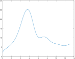
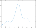
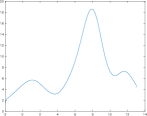
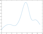
Figure 2: Scale-space signatures computed at corresponding central points for three images of a poster taken from different distances. Each scale-space signature shows the variation over scale of the scale-normalized quasi quadrature measure at the center as function of effective scale approximated by $s_{eff}=\log_{2}(s_{0}+s)$ for $s_{0}=1/8$. (middle column) the unsmoothed quasi quadrature measure ${\cal Q}_{(x,y),\Gamma-norm}L$ using $\Gamma_{s}=1/4$. (right column) the post-smoothed quasi quadrature measure $\overline{\cal Q}_{(x,y),\Gamma-norm}L$ using $\Gamma_{s}=1/4$ and $c=1$. Note how the scale levels at which the local maxima over scale are assumed follow the size variations in the image domain caused by varying the distance between the camera and the poster. All results have been computed using $C_{s}=1/\sqrt{(1-\Gamma_{s})(2-\Gamma_{s})}$. (Scale range: $s\in[0.1,8192]$, Image size: $480\times 640$ pixels.)

2.1.3 Basic scale selection method

A basic method for dense scale selection does therefore consist of detecting local extrema over scale of either the pointwise scale-normalized quasi quadrature entity (8)

(14) $$\hat{s}_{{\cal Q}L}=\operatorname{argmaxlocal}_{s>0}{\cal Q}_{(x,y),\Gamma-norm}L$$

or the corresponding post-smoothed entity (11)

(15) $$\hat{s}_{\overline{\cal Q}L}=\operatorname{argmaxlocal}_{s>0}\overline{\cal Q}_{(x,y),\Gamma-norm}L.$$

Figure 2 illustrates the effects of these operations for three different images of the same poster taken for different distances between the poster and the camera. As can be seen from the graphs, the scale values at which the local extrema over scale are assumed adapt to the size variations in the image domain and are assumed at coarser scales relative to the fixed image resolution as the camera approaches the object.

2.2 Scale selection properties

When applying this methodology in practice, there are a number of additional issues that need to be considered, which we will illustrate by closed form theoretical analysis using idealized image models representing a dense texture pattern or sparse image features respectively.

2.2.1 Two-dimensional sine wave

For a two-dimensional sine wave

(16) $$f(x,y)=\sin(\omega_{0}x)+\sin(\omega_{0}y),$$

the scale-space representation can be computed in closed form

(17) $$L(x,y;\;t)=e^{-\omega_{0}^{2}s/2}(\sin(\omega_{0}x)+\sin(\omega_{0}y)).$$

If we disregard the spatial post-smoothing step by setting the proportionality parameter $c$ between the local scale parameter and the integration scale parameter to $c=0$, then the quasi quadrature entity assumes the form

$$\begin{split}{\cal Q}_{(x,y),\Gamma-norm}L=&\omega_{0}^{2}e^{-\omega_{0}^{2}s}s^{1-\Gamma_{s}}\times\end{split}$$

(18) $$\begin{split}&\left(\cos^{2}(\omega_{0}x)+\cos^{2}(\omega_{0}y)+C_{s}\omega_{0}^{2}s\left(\sin^{2}(\omega_{0}x)+\sin^{2}(\omega_{0}y)\right)\right).\end{split}$$

By differentiating this expression with respect to scale $s$, it follows that for the image points $(x,y)=(m\pi/\omega_{0},n\pi/\omega_{0})$ at which only the first-order component

(19) $${\cal Q}_{(x,y),1,\Gamma-norm}L=\frac{|\nabla_{norm}L|^{2}}{s^{\Gamma_{s}}}=\frac{s\,(L_{x}^{2}+L_{y}^{2})}{s^{\Gamma_{s}}}$$

responds, the local extrema over scales are assumed at

(20) $$\hat{s}_{1}=\frac{1-\Gamma_{s}}{\omega_{0}^{2}}.$$

Correspondingly, for the spatial positions $(x,y)=((\pi/2+m\pi)/\omega_{0},(\pi/2+n\pi)/\omega_{0})$ at which only the second-order component

(21) $${\cal Q}_{(x,y),2,\Gamma-norm}L=\frac{C_{s}\,\|{\cal H}_{norm}L\|_{F}^{2}}{s^{\Gamma_{s}}}=\frac{C_{s}\,s^{2}\;(L_{xx}^{2}+2L_{xy}^{2}+L_{yy}^{2})}{s^{\Gamma_{s}}}$$

responds, the local extrema are assumed at

(22) $$\hat{s}_{2}=\frac{2-\Gamma_{s}}{\omega_{0}^{2}}.$$

In this respect, the combination of first- and second-order derivatives in the quasi quadrature entity will lead to a strong phase dependency in the scale estimates.

At the intermediate points $(x,y)=((\pi/4+m\pi/2)/\omega_{0},(\pi/4+n\pi/2)/\omega_{0})$, the scale estimate is given by

(23) $$\hat{s}_{intermed}=\frac{\sqrt{C_{s}^{2}(\Gamma_{s}-2)^{2}-2C_{s}\Gamma_{s}+1}-C_{s}(\Gamma_{s}-2)-1}{2C_{s}\omega_{0}^{2}}.$$

If we require the scale estimates at the intermediate points to be equal to the geometric average of the extreme cases

(24) $$\hat{s}_{intermed}=\sqrt{\hat{s}_{1}\,\hat{s}_{2}}=\frac{\sqrt{(1-\Gamma_{s})(2-\Gamma_{s})}}{\omega_{0}^{2}},$$

then this implies that $C_{s}$ should be chosen as

(25) $$C_{s}=\frac{1}{2-\Gamma_{s}}.$$

Alternatively, if we determine the weighting parameter $C_{s}$ such that the relative strengths of the first- and second-order components become equal at the midpoints $(x,y)=(\pi/4+m\pi/2)/\omega_{0},\pi/4+m\pi/2)/\omega_{0})$ between the extreme points for the scale corresponding to the geometric average $\sqrt{\hat{s}_{1}\,\hat{s}_{2}}$ of the extreme values

(26) $$\left.{\cal Q}_{(x,y),1,\Gamma-norm}L\right|_{x=\frac{\pi}{4\omega_{0}},y=\frac{\pi}{4\omega_{0}},s=\sqrt{\hat{s}_{1}\,\hat{s}_{2}}}=\left.{\cal Q}_{(x,y),2,\Gamma-norm}L\right|_{x=\frac{\pi}{4\omega_{0}},y=\frac{\pi}{4\omega_{0}},s=\sqrt{\hat{s}_{1}\,\hat{s}_{2}}},$$

then this implies that the relative weighting factor $C_{s}$ between the first- and second-order derivative responses should be chosen as

(27) $$C_{s}=\frac{1}{\sqrt{(1-\Gamma_{s})(2-\Gamma_{s})}}.$$

	Dense scale selection without post-smoothing
	$\Gamma_{s}=0$	$\Gamma_{s}=\frac{1}{4}$	$\Gamma_{s}=\frac{1}{2}$
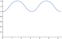
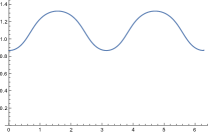
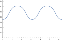
	Phase-compensated dense scale selection without post-smoothing
	$\Gamma_{s}=0$	$\Gamma_{s}=\frac{1}{4}$	$\Gamma_{s}=\frac{1}{2}$
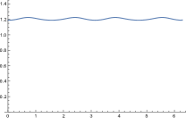
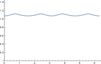
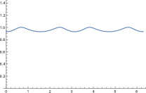
	Dense scale selection with post-smoothing
	$\Gamma_{s}=0$	$\Gamma_{s}=\frac{1}{4}$	$\Gamma_{s}=\frac{1}{2}$
$c=1/\sqrt{2}$
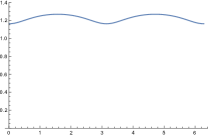
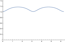
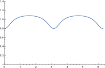
$c=1$
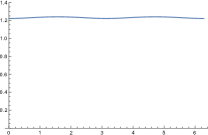
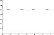
$c=\sqrt{2}$

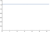
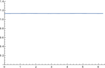
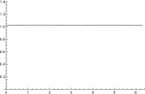
Figure 3: Spatial variability of the local scale estimates in units of $\sigma_{s}=\sqrt{s}$ for a 1-D sine wave $f(x)=\sin\omega_{0}x$ with angular frequency $\omega_{0}=1$: (top row) regular scale estimates without post-smoothing according to (14), (second row) phase-compensated scale estimates on a logarithmic scale and without post-smoothing according to (LABEL:eq-scale-phasecorr-geom-sine-tau), (third, fourth and bottom rows) scale estimates computed from local extrema over scale of the post-smoothed quasi quadrature entity $\overline{\cal Q}_{(x,y),\Gamma-norm}L$ according to (15) for relative post-smoothing scales $c=1/\sqrt{2}$, $c=1$ and $c=\sqrt{2}$, respectively. (All results have been computed using $C_{s}=1/\sqrt{(1-\Gamma_{s})(2-\Gamma_{s})}$.)

2.3 Phase-compensated scale estimate

Given this understanding of how the scale estimates depend on the local phase of a sine wave, we can define a phase-compensated scale estimate according to either

$$\begin{split}\hat{s}_{{\cal Q}L,comp}=&\frac{\sqrt{(1-\Gamma_{s})(2-\Gamma_{s})}}{\left({\cal Q}_{(x,y),1,\Gamma-norm}L+{\cal Q}_{(x,y),2,\Gamma-norm}L\right)}\times\end{split}$$

(28) $$\begin{split}&\left(\frac{{\cal Q}_{(x,y),1,\Gamma-norm}L}{1-\Gamma_{s}}+\frac{{\cal Q}_{(x,y),2,\Gamma-norm}L}{2-\Gamma_{s}}\right)\,\hat{s}_{{\cal Q}L}\end{split}$$

or

$$\begin{split}&\hat{s}_{{\cal Q}L,comp}=\end{split}$$

$$\begin{split}&\frac{\sqrt{(1-\Gamma_{s})(2-\Gamma_{s})}}{(1-\Gamma_{s})^{\frac{{\cal Q}_{(x,y),1,\Gamma-norm}L}{{\cal Q}_{(x,y),1,\Gamma-norm}L+{\cal Q}_{(x,y),2,\Gamma-norm}L}}(2-\Gamma_{s})^{\frac{{\cal Q}_{(x,y),2,\Gamma-norm}L}{{\cal Q}_{(x,y),1,\Gamma-norm}L+{\cal Q}_{(x,y),2,\Gamma-norm}L}}}\,\hat{s}_{{\cal Q}L}.\end{split}$$

These expressions are defined to be equal to the geometric average

(30) $$\hat{s}_{geom}=\sqrt{\hat{s}_{1}\,\hat{s}_{2}}=\frac{\sqrt{(1-\Gamma_{s})(2-\Gamma_{s})}}{\omega_{0}^{2}}$$

of the extreme values when only one of the first- or second-order components in ${\cal Q}_{\Gamma-norm}L$ responds and using blending of these responses by transfinite interpolation [13] using the relative strengths of the first- and second-order responses, respectively, to achieve a much lower variability of the scale estimates in between (see Figure 3).

The motivation to the definitions of equations (2.3) and (LABEL:eq-scale-phasecorr-geom-sine-tau) is to express interpolation functions on a simple form that compensate for the phase dependency of the scale estimates depending on the relative strengths of the first- and second-order components. When only the first-order component responds and the second-order component is zero, the scale estimate is $\hat{s}_{1}=(1-\Gamma_{s})/\omega_{0}^{2}$. When only the second-order component responds and the first-order component is zero, the scale estimate is $\hat{s}_{2}=(2-\Gamma_{s})/\omega_{0}^{2}$.

In the first expression (2.3), the ratios $w_{1}={\cal Q}_{(x,y),1,\Gamma-norm}L/({\cal Q}_{(x,y),1,\Gamma-norm}L+{\cal Q}_{(x,y),2,\Gamma-norm})$ and $w_{2}={\cal Q}_{(x,y),2,\Gamma-norm}L/({\cal Q}_{(x,y),1,\Gamma-norm}L+{\cal Q}_{(x,y),2,\Gamma-norm})$, which are positive and sum to one $w_{1}+w_{2}=1$, are used as relative weights in a a linear convex combination

(31) $$\hat{s}_{comp}=s_{geom}\left(w_{1}\,\frac{\hat{s}}{\hat{s}_{1}}+w_{2}\,\frac{\hat{s}}{\hat{s}_{2}}\right)$$

defined such that $\hat{s}_{comp}=s_{geom}$ if either $(w_{1}=1,w_{2}=0,\hat{s}=\hat{s}_{1})$ or $(w_{1}=0,w_{2}=1,\hat{s}=\hat{s}_{2})$. In the second expression (LABEL:eq-scale-phasecorr-geom-sine-tau), the same ratios $w_{1}$ and $w_{2}$ are used as relative weights in a a geometric convex combination

(32) $$\hat{s}_{comp}=s_{geom}\left(\frac{\hat{s}}{\hat{s}_{1}}\right)^{w_{1}}\left(\frac{\hat{s}}{\hat{s}_{2}}\right)^{w_{2}}$$

again defined such that $\hat{s}_{comp}=s_{geom}$ if either $(w_{1}=1,w_{2}=0,\hat{s}=\hat{s}_{1})$ or $(w_{1}=0,w_{2}=1,\hat{s}=\hat{s}_{2})$.

For the first expression (2.3), the blending is thus performed on a linear scale with respect to the spatial scale parameter, whereas the blending is performed on a more natural logarithmic scale in the second expression (LABEL:eq-scale-phasecorr-geom-sine-tau).

From these spatial scale estimates, we can in turn estimate the temporal wavelength of the sine wave according to

(33) $$\hat{\lambda}=\frac{2\pi\sqrt{\hat{s}_{{\cal Q}_{L},comp}}}{\sqrt[4]{(1-\Gamma_{s})(2-\Gamma_{s})}}.$$

Whereas the interpolation functions (2.3) and (LABEL:eq-scale-phasecorr-geom-sine-tau) in combination with (33) will not lead to exact wavelength estimates for all phases of a sine wave, these functions compensate for the gross behaviour of the phase dependency, which substantially decreases the otherwise much higher spatial variability in the spatial scale estimates.

2.4 Scale calibration

In Sections 2.2–2.3 as well as a more detailed analysis in the appendix, it is shown how the scale estimates $\hat{s}_{{\cal Q}L}$ and $\hat{s}_{\overline{\cal Q}L}$ according to (14) and (15) are influenced by the parameters $\Gamma_{s}$, $c$ and $C_{s}$ in the quasi quadrature measure. To decouple this dependency from the later stage visual modules for which the dense scale selection methodology is intended to be used as an initial pre-processing stage, we introduce the notion of scale calibration, which implies that the scale estimates are to be multiplied by uniform scaling factors such that they are either:

• equal to the scale estimate $\hat{s}=s_{0}$ obtained by applying the regular scale-normalized Laplacian $\nabla_{norm}^{2}L=s\,(L_{xx}+L_{yy})$ or the scale-normalized determinant of the Hessian $\det{\cal H}_{norm}L=s^{2}\,(L_{xx}L_{yy}-L_{xy}^{2})$ at the center of a Gaussian blob of any spatial extent $s_{0}$ or

• equal to the scale estimate $\hat{s}=\sqrt{2}/\omega_{0}^{2}$ corresponding to the geometric average of the scale estimates obtained for a sine wave of any angular frequency $\omega_{0}$ when $\Gamma_{s}=0$.

The first method, which aims at similarity with previous scale selection methods at sparse image features, will be referred to as Gaussian scale calibration, whereas the second method, which aims at similarity for dense texture patterns, will be referred to as sine wave scale calibration.

The necessary calibration factors can for the cases of either (i) no phase compensation and no post-smoothing or (ii) phase compensation without post-smoothing be obtained from the theoretical results in section 2.2. Ways of deriving the scale calibration factors when using spatial post-smoothing are described in the appendix.

2.5 Composed dense scale selection algorithms

Given the above treatment, we can define four types of dense scale selection algorithms:

Algorithm I:

Without post-smoothing or phase compensation, with local scale estimates at every image point computed according to (14).

Algorithm II:

With phase compensation and without post-smoothing, with local scale estimates at every image point computed according to (2.3) or (LABEL:eq-scale-phasecorr-geom-sine-tau) based on uncompensated local scale estimates according to (14).

Algorithm III:

With post-smoothing and without phase compensation, with local scale estimates at every image point computed according to (15).

Algorithm IV:

With both post-smoothing and phase compensation, with local phase-compensated scale estimates at every image point computed in an analogous way as (2.3) or (LABEL:eq-scale-phasecorr-geom-sine-tau) although based on post-smoothing according (15) and with the factors $(1-\Gamma_{s})$ and $(2-\Gamma_{s})$ in the expressions for phase compensation, which originate from the local extrema over scale when $c=0$, replaced by $S_{sine,1}(\Gamma_{s},c,C_{s})$ and $S_{sine,2}(\Gamma_{s},c,C_{s})$ according to (94) in the appendix.

The scale estimates from each algorithm can in turn be calibrated using either Gaussian scale calibration or sine wave calibration according to Section 2.4.

2.6 Scale covariance of the spatial scale estimates under spatial scaling transformations

Consider a scaling transformation of the spatial image domain

(34) $$f^{\prime}(x_{1}^{\prime},x_{2}^{\prime})=f(x_{1},x_{2})\quad\quad\mbox{for}\quad\quad(x_{1}^{\prime},x_{2}^{\prime})=(S_{s}\,x_{1},S_{s}\,x_{2}),$$

where $S_{s}$ denotes the spatial scaling factor. Define the spatial scale-space representations $L$ and $L^{\prime}$ of $f$ and $f^{\prime}$, respectively, according to

(35) $$\begin{split}&L(x_{1},x_{2};\;s)=\left(T(\cdot,\cdot;\;s)*f(\cdot,\cdot,)\right)(x_{1},x_{2};\;s),\end{split}$$

(36) $$\begin{split}&L^{\prime}(x^{\prime}_{1},x^{\prime}_{2};\;s^{\prime})=\left(T(\cdot,\cdot;\;s^{\prime})*f^{\prime}(\cdot,\cdot)\right)(x^{\prime}_{1},x^{\prime}_{2};\;s^{\prime}).\end{split}$$

Consider a spatial differential expression of the form

(37) $${\cal D}L=\sum_{i=1}^{I}\prod_{j=1}^{J}c_{i}\,L_{x^{\alpha_{ij}}}=\sum_{i=1}^{I}\prod_{j=1}^{J}c_{i}\,L_{x_{1}^{\alpha_{1ij}}x_{2}^{\alpha_{2ij}}},$$

required to be homogeneous in the sense that the sum of the orders of differentiation in each term does not depend on the index of that term

(38) $$\sum_{j=1}^{J}|\alpha_{ij}|=\sum_{j=1}^{J}\alpha_{1ij}+\alpha_{2ij}=M.$$

Then, the corresponding homogeneous differential expression ${\cal D}_{norm}L$ with the spatial derivatives $L_{x_{1}^{m_{1}}x_{2}^{m_{2}}}$ replaced by scale-normalized derivatives according to

(39) $$L_{\xi_{1}^{m_{1}}\xi_{2}^{m_{2}}}=s^{(m_{1}+m_{2})\gamma_{s}/2}\,L_{x_{1}^{m_{1}}x_{2}^{m_{2}}},$$

transforms according to (Lindeberg [35, Equation (25)])

(40) $${\cal D^{\prime}}_{norm}L^{\prime}=S_{s}^{M(\gamma_{s}-1)}\,{\cal D}_{norm}L.$$

Regarding the spatial quasi quadrature measure ${\cal Q}_{(x,y),\Gamma-norm}L$ according to (8) that we use for dense spatial scale selection, this differential invariant is not homogeneous of the form (37). If we split this differential expression into two components based on the orders of spatial differentiation

(41) $$\begin{split}{\cal Q}_{(x,y),\Gamma-norm}L=&{\cal Q}_{(x,y),1,\Gamma-norm}L+{\cal Q}_{(x,y),2,\Gamma-norm}L\end{split}$$

where

(42) $$\begin{split}{\cal Q}_{(x,y),1,\Gamma-norm}L&=\frac{s\,(L_{x}^{2}+L_{y}^{2})}{s^{\Gamma_{s}}},\end{split}$$

(43) $$\begin{split}{\cal Q}_{(x,y),2,\Gamma-norm}L&=\frac{C_{s}\,s^{2}\,\left(L_{xx}^{2}+2L_{xy}^{2}+L_{yy}^{2}\right)}{s^{\Gamma_{s}}},\end{split}$$

we can note that each one of these expressions is of the homogeneous form (37) and corresponds to $\gamma$-normalized scale-space derivatives in the respective cases:

(44) $$\gamma_{1}=1-\Gamma_{s},\quad\quad\gamma_{2}=1-\frac{\Gamma_{s}}{2}.$$

Applying the transformation property (40) to each of the two components of the spatial quasi quadrature measure, then gives that they transform according to

(45) $$\begin{split}{\cal Q}_{(x^{\prime},y^{\prime}),1,\Gamma-norm}L^{\prime}&=S_{s}^{2(\gamma_{1}-1)}\,{\cal Q}_{(x,y),1,\Gamma-norm}L=S_{s}^{-2\Gamma_{s}}\,{\cal Q}_{(x,y),1,\Gamma-norm}L,\end{split}$$

(46) $$\begin{split}{\cal Q}_{(x^{\prime},y^{\prime}),2,\Gamma-norm}L^{\prime}&=S_{s}^{2\times 2(\gamma_{2}-2)}\,{\cal Q}_{(x,y),2,\Gamma-norm}L=S_{s}^{-2\Gamma_{s}}\,{\cal Q}_{(x,y),2,\Gamma-norm}L.\end{split}$$

In other words, because of the deliberate adding of differential expressions corresponding to different orders of spatial differentiation for the maximally scale invariant case of $\gamma_{s}=1$ prior to post-normalization by the post-normalization power $\Gamma_{s}$, it follows that the two components transform in the same way under spatial scaling transformations, implying that the composed quasi quadrature measure transforms as

(47) $$({\cal Q}_{(x^{\prime},y^{\prime}),\Gamma-norm}L^{\prime})(x^{\prime},y^{\prime};\;s^{\prime})=S_{s}^{-2\Gamma_{s}}\,({\cal Q}_{(x,y),\Gamma-norm}L)(x,y;\;s)$$

under uniform scaling transformations of the spatial image domain.

This covariance property under spatial scaling transformations does specifically imply that local extrema over spatial scales are preserved under uniform scaling transformations of the spatial image domain and are transformed in a scale-covariant way

(48) $$\hat{s}^{\prime}=S_{s}^{2}\,\hat{s}$$

or in units of the standard deviation $\sigma_{s}=\sqrt{s}$ of the spatial scale-space kernel

(49) $$\hat{\sigma}^{\prime}_{s}=S_{s}\,\hat{\sigma}_{s}.$$

This property constitutes the theoretical foundation for dense spatial scale selection and implies that the local spatial scale estimates will automatically adapt to local variations in the dominant spatial scales in the image data.

This scale covariance of the spatial scale estimates does also extend to phase-compensated scale estimates according to (2.3) or (LABEL:eq-scale-phasecorr-geom-sine-tau). This property is straightforward to prove, since the underlying uncompensated spatial scale estimates $\hat{s}_{{\cal Q}L}$ in (2.3) or (LABEL:eq-scale-phasecorr-geom-sine-tau) are provably scale covariant and additionally the ratio that determines the scale compensation factor is invariant under independent scaling transformations of the spatial domain provided that the spatial scale levels are appropriately matched, which they are if the phase compensation factors are computed at scale levels corresponding to the spatial scale estimates.

Correspondingly, the scale covariance of the spatial scale estimates also extends to spatial post-smoothing prior to the detection of local extrema over spatial scales. This property follows from the fact that the amount of spatial post-smoothing is proportional to the spatial scale level at which the non-linear quasi quadrature measure is computed.

Under affine intensity transformations

(50) $$f^{\prime}(x,y)=a\,f(x,y)+b,$$

the Gaussian derivatives are multiplied by a uniform scaling factor $L^{\prime}_{x^{\alpha}y^{\beta}}(x,y;\;t)=a\,L_{x^{\alpha}y^{\beta}}(x,y;\;t)$ and the quasi quadrature measure transforms according to

(51) $${\cal Q}^{\prime}_{(x,y),\Gamma-norm}(x,y;\;s)=a^{2}\,{\cal Q}_{(x,y),\Gamma-norm}(x,y;\;s).$$

The scale estimates are therefore unaffected by illumination variations whose effects can be well approximated by local affine transformations over the intensity domain.

The spatial quasi quadrature entities used for scale selection are based on the rotationally invariant differential invariants $|\nabla L|^{2}$ and $\|{\cal H}L\|^{2}$ and are therefore rotationally invariant. This implies that the resulting scale spatial estimates are covariant under rotations of the spatial image domain.

Original image	Dense scale estimates using Algorithm II

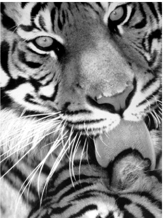
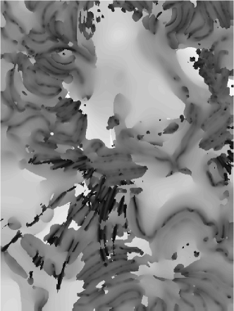
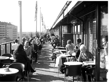
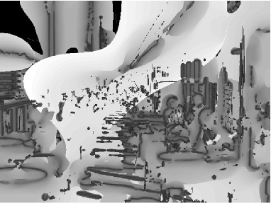
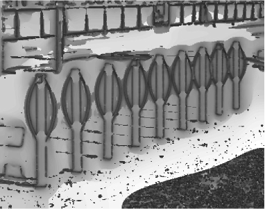
Figure 4: Dense spatial scale maps computed using Algorithm II (dense scale selection with phase compensation) for three different images using $\Gamma_{s}=1/4$ and $C_{s}=1/\sqrt{(1-\Gamma_{s})(2-\Gamma_{s})}$. The grey-levels code for effective scale approximated by $s_{eff}=\log_{2}(s_{0}+s)$ for $s_{0}=1/8$ in such a way that darker means finer spatial scales and brighter indicates coarser spatial scales. See Section 2.7 for more detailed explanations. Observe, however, that for the quite common phenomenon when there are multiple local extrema over scale corresponding to different types of dominant structures at different scales, this visualization only shows the one of the scale estimates that has the strongest maximum response. Thereby, situations where the maximum value over scales switches between two scale selection surfaces at difference scales appear as discontinuities in this simplified form of visualization. Such layer discontinuities are therefore artefacts of the visualization method — not the scale selection method. A more appropriate form of visualization is in terms of a 3-D visualization of the scale selection surfaces as shown in Figure 5, where multiple scale estimates may be displayed at every image point.

Original image

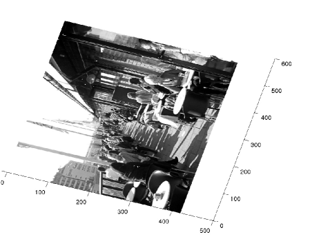
Scale selection surfaces from $\partial_{s}({\cal Q}_{(x,y),\Gamma-norm}L)=0$ painted with $L$.

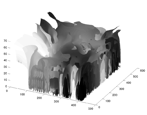
Scale selection surfaces from $\partial_{s}({\cal Q}_{(x,y),\Gamma-norm}L)=0$ painted with $f$.

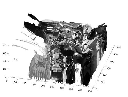
Figure 5: 3-D visualization of local scale estimates underlying the dense scale maps shown in Figure 4(right) and shown as scale selection surfaces in 3-D scale space over space $(x,y)$ and scale $s$, here also visualizing multiple local extrema over scales at every image point. (Scale values in units of effective scale approximated by $s_{eff}=\log_{2}(s_{0}+s)$ for $s_{0}=1/8$.)

2.7 Experimental results

Figure 4 shows spatial scale maps computed using Algorithm II for three images. All the scale maps have been computed using Gaussian scale calibration for $\Gamma_{s}=1/4$. For all images in this illustration, we can note how finer scale estimates are selected near edges, leading to a sketch-like representation of prominent edges. This behaviour is in good agreement with the theory and does also imply that image features or image descriptors that are computed with this type of scale selection methodology will be well localized near edges.

In general, the detection of local extrema over scale of the quasi quadrature entity ${\cal Q}_{(x,y),\Gamma-norm}L$ will sweep out scale selection surfaces defined by

(52) $$\left\{\begin{array}[]{l}\partial_{s}({\cal Q}_{(x,y),\Gamma-norm}L)=0\\ \partial_{ss}({\cal Q}_{(x,y),\Gamma-norm}L)<0\end{array}\right.$$

in the 3-D scale space spanned by the spatial dimensions $(x,y)$ and the scale parameter $s$. Specifically, when the local image structures contain different types of structures at different scales, multiple local extrema over scale may be detected, corresponding to multiple patches of the scale selection surfaces at different scales, which may represent qualitatively different types of image structures in the image domain while at different scales.

In Figure 4, a very much simplified form of visualization has been used, by only showing the scale value of the local maximum over scale that has the maximum response among the possibly multiple local maxima over scale. When moving between different points over the spatial domain, this global maximum may at some places switch between different patches of the scale selection surfaces at different scales. The discontinuities in the scale maps that can be seen in the right column correspond to such switching between multiple scale selection surfaces and are artefacts of the visualization method, not the scale selection method.

More generally, one should of course treat multiple local extrema over scale as multiple scale hypotheses as done in the more appropriate 3-D visualization of such multiple scale selection surfaces in Figure 5. From a more detailed inspection of the scale selection surface patch corresponding to the edge of the roof in the upper part of the image, one can also find that the selected scale levels decrease with increasing distance from the camera as caused by perspective effects. The similarities between the scale maps for the repetitive structures in the image in the lower part of the figure demonstrate the stability of the dense scale estimates under natural imaging conditions, whereas the relative differences in scale estimates between corresponding parts of the different but similar looking pillars reveal the size gradient caused by perspective scaling effects.

To quantify the numerical stability of the scale estimates for a stimulus for which the scale estimates should be approximately constant, we computed dense scale estimates for a set of 2-D sine waves of the form

(53) $$f(x,y)=\sin\omega x+\sin\omega y$$

with wavelengths $\lambda=8,16,32$ and $64$ for each one of the four types of algorithms and compared the results with corresponding theoretical predictions based on the scale selection properties of the 1-D sine wave model (24)

(54) $$\hat{\omega}=\frac{\sqrt[4]{(1-\Gamma_{s})(2-\Gamma_{s})}}{\sqrt{\hat{s}}}.$$

The mean and the standard deviation around the mean were computed for the scale estimates in terms of effective scale $s_{eff}$ and these measures were transformed into relative measures in units the scale parameter $\sigma_{s}=\sqrt{s}$ of dimension $[\mbox{length}]$. As can be seen from the results in Table 1, the use of phase compensation and complementary post-smoothing substantially decreases the spatial variability in the scale estimates by an order of magnitude in units of $\sigma_{s}$. Specifically, pure phase compensation achieves a a reduction in the variability of the same order as pure post-smoothing for $c=1$, while also allowing for a higher resolution in the scale estimates near edge-like structures.

Accuracy of scale estimates for a 2-D sine wave pattern
Error measure	Alg. I	Alg. II	Alg. III	Alg. IV
Offset of mean	+ 5.0 %	- 0.6 %	+ 1.6 %	+ 1.5 %
Relative spread	$\pm$ 11.8 %	$\pm$ 1.3 %	$\pm$ 0.6 %	$\pm$ 0.1 %

Table 1: Measures of the accuracy of the scale estimates computed for a 2-D sine wave $f(x,y)=\sin\omega x+\sin\omega y$ and compared to corresponding theoretical predictions based on a 1-D sine wave model according to (33) for Algorithms I–IV using $\Gamma_{s}=1/4$, $c=1$ and $C_{s}=1/\sqrt{(1-\Gamma_{s})(2-\Gamma_{s})}$.

3 Dense temporal scale selection over a purely temporal domain

In this section, we develop a corresponding approach for dense scale selection over a purely temporal domain.

3.1 A temporal quasi quadrature measure

Motivated by the fact that first-order derivatives respond primarily to the locally odd component of a signal, whereas second-order derivatives respond primarily to the locally even component of a signal, it is for dense applications natural to aim at a feature detector that combines such first- and second-order temporal derivative responses. By specifically combining the squares of the first- and second-order temporal derivative responses in an additive way, we obtain a temporal quasi quadrature measure of the form

(55) $${\cal Q}_{t,\Gamma-norm}L=\frac{\tau L_{t}^{2}+C_{\tau}\tau^{2}L_{tt}^{2}}{\tau^{\Gamma_{\tau}}},$$

which is a reduction of the 2-D spatial quasi quadrature measure (8) to a 1-D purely temporal domain, where $t$ denotes time and $\tau$ temporal scale.

This construction is closely related to a proposal by Koenderink and van Doorn [29] of summing up the squares of the first- and second-order derivative responses of receptive fields and an observation by De Valois et al. [65] that first- and second-order biological receptive fields typically occur in pairs that can be modelled as approximate Hilbert pairs, while here instead formalized in terms of scale-normalized temporal scale-space derivatives.

3.2 Scale covariance of temporal scale estimates under temporal scaling transformations

Consider a temporal scaling transformation of the form

(56) $$f^{\prime}(t^{\prime})=f(t)\quad\quad\mbox{for}\quad\quad t^{\prime}=S_{\tau}\,t.$$

From the temporal scaling transformation of scale-normalized temporal derivatives defined from either the non-causal Gaussian temporal scale space or the time-causal temporal scale space obtained by convolution with the time-causal limit kernel [43], it follows that scale-normalized temporal derivatives of order $n$ are transformed according to [46, Equations (10) and (104)]

(57) $$\partial_{\zeta^{\prime n},{norm}}L^{\prime}(t^{\prime};\;\tau^{\prime})=S_{\tau}^{n(\gamma_{\tau}-1)}\,\partial_{\zeta^{n},{norm}}L(t;\;\tau)$$

provided that the temporal scale levels are correspondingly matched

(58) $$\tau^{\prime}=S_{\tau}^{2}\,\tau.$$

Applied to the temporal quasi quadrature measure

(59) $${\cal Q}_{t,\Gamma-norm}L=\frac{\tau L_{t}^{2}+C_{\tau}\tau^{2}L_{tt}^{2}}{\tau^{\Gamma_{\tau}}}={\cal Q}_{t,1,\Gamma-norm}L+{\cal Q}_{t,2,\Gamma-norm}L$$

with its first- and second-order components

(60) $${\cal Q}_{t,1,\Gamma-norm}L=\frac{\tau L_{t}^{2}}{\tau^{\Gamma_{\tau}}},\quad\quad{\cal Q}_{t,2,\Gamma-norm}L=\frac{C_{\tau}\tau^{2}L_{tt}^{2}}{\tau^{\Gamma_{\tau}}},$$

and which correspond to $\gamma$-normalized temporal derivatives with $\gamma_{1}=1-\Gamma_{\tau}$ and $\gamma_{2}=1-\Gamma_{\tau}/2$ for the first- and second-order components, respectively, it follows that the first- and second-order components transform according to

$$\begin{split}({\cal Q}_{t,1,\Gamma-norm}L^{\prime})(t^{\prime};\;\tau^{\prime})&=S_{\tau}^{2(\gamma_{1}-1)}\,({\cal Q}_{t,1,\Gamma-norm}L)(t;\;\tau)\end{split}$$

(61) $$\begin{split}&=S_{\tau}^{-2\Gamma_{\tau}}\,({\cal Q}_{t,1,\Gamma-norm}L)(t;\;\tau),\end{split}$$

$$\begin{split}({\cal Q}_{t,2,\Gamma-norm}L^{\prime})(t^{\prime};\;\tau^{\prime})&=S_{\tau}^{2\times 2(\gamma_{2}-1)}\,({\cal Q}_{t,2,\Gamma-norm}L)(t;\;\tau)\end{split}$$

(62) $$\begin{split}&=S_{\tau}^{-2\Gamma_{\tau}}\,({\cal Q}_{t,2,\Gamma-norm}L)(t;\;\tau).\end{split}$$

Since the first- and second-order components transform in a similar way because of the deliberate adding of entities depending on temporal derivatives of different orders for the maximally scale-invariant choice of $\gamma_{\tau}=1$, it follows that the temporal quasi quadrature measure despite its inhomogeneity still transforms according to a power law

(63) $$({\cal Q}_{t,\Gamma-norm}L^{\prime})(t^{\prime};\;\tau^{\prime})=S_{\tau}^{-2\Gamma_{\tau}}\,({\cal Q}_{t,\Gamma-norm}L)(t;\;\tau).$$

Specifically, this implies that temporal scale estimates computed from local extrema over temporal scales are preserved and are transformed in a scale covariant way

(64) $$\hat{\tau}^{\prime}=S_{\tau}^{2}\,\hat{\tau}$$

or in units of the standard deviation $\sigma_{\tau}=\sqrt{\tau}$ of the temporal scale-space kernel

(65) $$\hat{\sigma}^{\prime}_{\tau}=S_{\tau}\,\hat{\sigma}_{\tau}.$$

This does in turn imply that the temporal scale estimates will adapt to local temporal scaling transformations of the input signal, and constitutes the theoretical basis for the dense temporal scale selection methodology.

This temporal scale covariance property does also extend to phase-compensated temporal scale estimates according to (LABEL:eq-scale-phasecorr-geom-sine-tau)

(66) $$\begin{split}\hat{\tau}_{{\cal Q}_{t},comp}&=\frac{\sqrt{(1-\Gamma_{\tau})(2-\Gamma_{\tau})}\,\hat{\tau}_{{\cal Q}_{t}}}{(1-\Gamma_{\tau})^{\frac{{\cal Q}_{t,1,\Gamma-norm}L}{{\cal Q}_{t,1,\Gamma-norm}L+{\cal Q}_{t,2,\Gamma-norm}L}}(2-\Gamma_{\tau})^{\frac{{\cal Q}_{t,2,\Gamma-norm}L}{{\cal Q}_{t,1,\Gamma-norm}L+{\cal Q}_{t,2,\Gamma-norm}L}}},\end{split}$$

since the underlying uncompensated temporal scale estimates $\hat{\tau}_{{\cal Q}_{t}}$ transform in a scale-covariant way and the ratios $w_{1}={\cal Q}_{t,1,\Gamma-norm}L/({\cal Q}_{t,1,\Gamma-norm}L+{\cal Q}_{t,2,\Gamma-norm}L)$ and $w_{2}={\cal Q}_{t,2,\Gamma-norm}L/({\cal Q}_{t,1,\Gamma-norm}L+{\cal Q}_{t,2,\Gamma-norm}L)$ that determine the scale compensation factors are invariant under temporal scaling transformations, provided that the temporal scale levels are appropriately matched.

The temporal scale covariance of the temporal scale estimates is also preserved under temporal post-smoothing, since the amount of temporal post-smoothing is proportional to the local temporal scale for computing the temporal derivatives.

original signal	$\sqrt{{\cal Q}_{t,norm}L}$	basic scale selection	phase-compensated

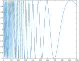
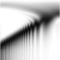
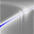
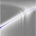
Figure 6: Dense temporal scale selection from local extrema over scale of the temporal quasi quadrature measure ${\cal Q}_{t,\Gamma-norm}L$ applied to a synthetic sine wave signal $f(t)=\sin(\exp((b-t)/a))$ for $a=200$ and $b=1000$ with temporally varying frequency so that the wavelength increases with time $t$. (left) Original temporal signal. (middle left) The square root of the temporal quasi quadrature measure ${\cal Q}_{t,\Gamma-norm}L$ computed for the most scale-invariant choice of the complementary scale normalization parameter $\Gamma_{\tau}=0$. (middle right) Basic scale estimates $\hat{\tau}_{{\cal Q}_{t,\Gamma-norm}}$ from local extrema over scale of the quasi quadrature measure according to (14) reduced to 1-D for $\Gamma_{\tau}=0$ and shown as blue curves overlaid on the magnitude map ${\cal Q}_{t,\Gamma-norm}L$ with reversed contrast. (right) Phase-compensated scale estimates $\hat{\tau}_{{\cal Q}_{t},comp}$ according to (LABEL:eq-scale-phasecorr-geom-sine-tau) reduced to 1-D for $\Gamma_{\tau}=0$ and shown as blue curves overlaid on the magnitude map ${\cal Q}_{t,\Gamma-norm}L$ with reversed contrast. All results have been computed using $C_{\tau}=1/\sqrt{(1-\Gamma_{\tau})(2-\Gamma_{\tau})}$. (Horizontal axis: time $t\in[0,1000]$) (Vertical axis in columns 2-4: effective temporal scale $\tau_{eff}=\log\tau$ over the range from $\sigma_{\tau,min}=0.25$ to $\sigma_{\tau,max}=1000$ for $\sigma_{\tau}=\sqrt{\tau}$)

post-smoothed scale selection (off med.)	post-smoothed scale selection (on med.)
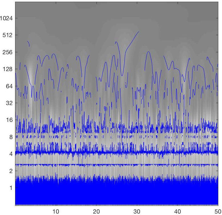
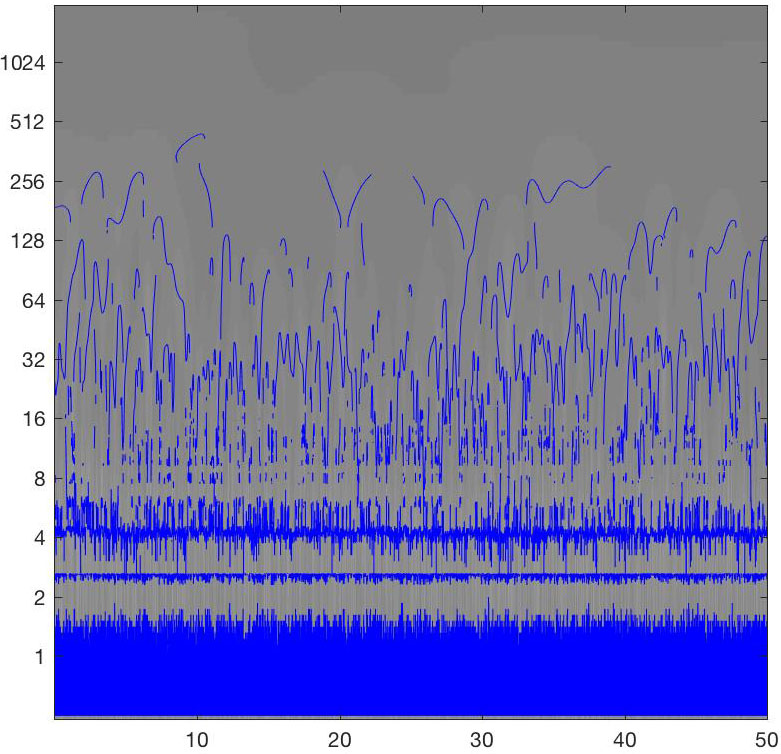
$\sqrt{{\cal Q}_{t,norm}L}$ Gaussian kernel (off med.)	$\sqrt{{\cal Q}_{t,norm}L}$ Gaussian kernel (on med.)
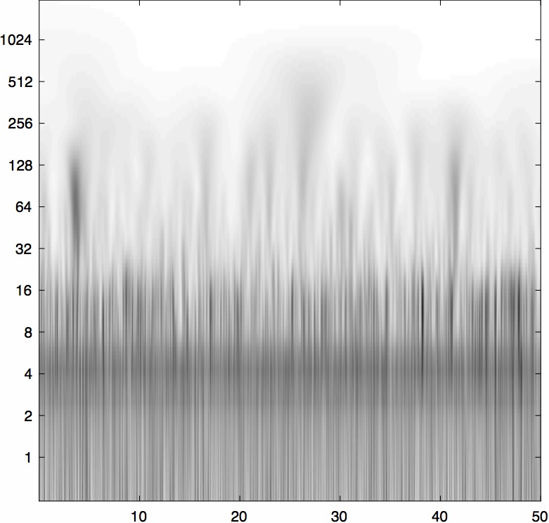
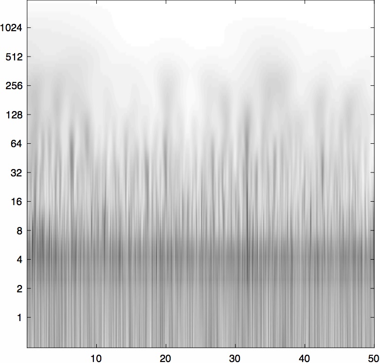
Original signal (off med.)	Original signal (on med.)

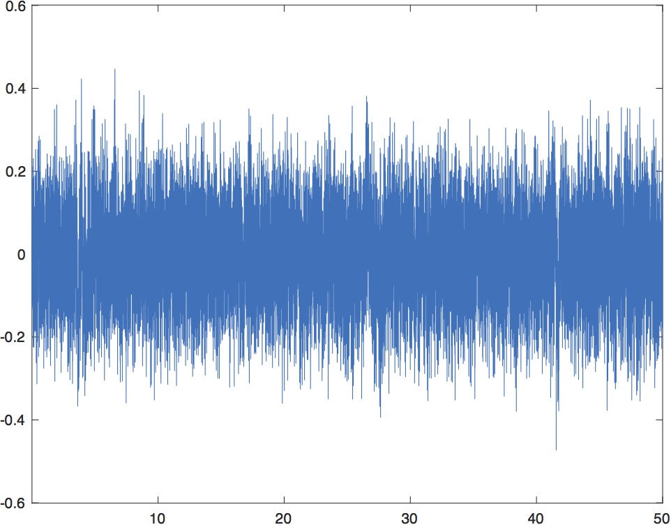
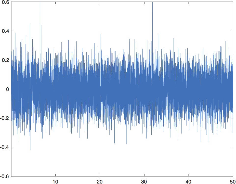
Figure 7: Dense local scale analysis of a neurophysiological signal from Caghan et al. [7] showing the local field potential sampled at $\nu=512$ Hz during 50 seconds for an electrode inserted in the sub-thalamic nucleus of an awake human subject with Parkinson’s disease (left column) without medication or (right column) when the patient is on on medication by leva-dopa. Note how this local scale analysis method reveals that the uppermost stronger band of dense local scale estimates in the top left figure is spread out over a larger scale range in the top right figure as a result of the medication. (top row) Basic scale estimates $\hat{\tau}_{{\cal Q}_{t,\Gamma-norm}}$ from local extrema over scale of the quasi quadrature measure according to (15) reduced to 1-D for $c=3$ and $\Gamma_{\tau}=0$. (middle row) The square root of the temporal quasi quadrature measure ${\cal Q}_{t,\Gamma-norm}L$ computed for the most scale-invariant choice of the complementary scale normalization parameter $\Gamma_{\tau}=0$. (bottom row) Original temporal signal. All results have been computed using $C_{\tau}=1/\sqrt{(1-\Gamma_{\tau})(2-\Gamma_{\tau})}$. (Horizontal axis: time $t\in[0,50]$ in seconds.) (Vertical axis in top and middle rows: temporal scale in milliseconds.)

3.3 Experimental results

3.3.1 Sine wave with exponentially varying frequency

Figure 6 shows the result of applying this basic form of dense temporal scale selection to a sine wave with exponentially varying frequency of the form

(67) $$f(t)=\sin(\exp(\frac{(b-t)}{a}))$$

for $a=200$ and $b=1000$. The left figure shows the raw temporal signal. The middle left figure shows the magnitude map over time and temporal scales of the temporal quasi quadrature measure ${\cal Q}_{t,norm}L$ computed using a non-causal Gaussian temporal scale-space representation. The middle right figure shows temporal scale estimates computed as the zero-crossings of $\partial_{\tau}({\cal Q}_{t,\Gamma-norm}L)=0$ that satisfy the sign condition $\partial_{\tau\tau}({\cal Q}_{t,\Gamma-norm}L)<0$. These zero-crossings have been interpolated to higher accuracy along the temporal scale dimension than the sampling density over the temporal scales using parabolic interpolation [46, Equation (115)]. In the rightmost figure, the basic temporal estimates from the middle right column have been additionally phase-compensated according to (66).

Note how: (i) the temporal scale selection method is able to capture the rapid variations in the temporal scales in the signal and (ii) the phase compensation method substantially suppresses the phase dependency of the temporal scale estimates.

3.3.2 Real measurement signals

Figure 7 shows an example of performing this type of dense temporal scale selection analysis on two real measurements signals using the non-causal Gaussian temporal scale-space concept. The figures in the bottom row show measurements of the local field potential recorded from the sub-thalamic nucleus of an awake human subject with Parkinson’s disease with the patient either off or on medication by leva-dopa (labelled “off med.” or “on med.” and shown in the left and the right columns, respectively).

As can be seen from the dense local scale estimates in the top row, the dense scale analysis does (beyond a wide band of responses at finer scales up to temporal scale $\sigma_{\tau,0}=1.4$ ms) return three rather strong bands of coarser temporal scale estimates when the patient is off medication. These bands are assumed around temporal scales $\sigma_{\tau,1}=2.6$ ms, $\sigma_{\tau,2}=4.5$ ms and $\sigma_{\tau,4}=11$ ms with a weaker additional band at temporal scale $\sigma_{\tau,3}=7.9$ ms. According to the approximate expression (33) for the local scale estimate of a sine wave, these scale estimates correspond to frequencies $\nu=1/\lambda$ around $\nu_{0}=136$ Hz, $\nu_{1}=73$ Hz, $\nu_{2}=42$ Hz, $\nu_{3}=24$ Hz and $\nu_{4}=18$ Hz.

When the patient is on medication, the uppermost band of coarser scale estimates around $\sigma_{\tau,4}=11$ ms is replaced by a sparser set of dense local scale estimates over a wider scale range. $[\sigma_{\tau,5},\sigma_{\tau,6}]=[10,42]$ ms and corresponding to frequencies in the range $[\nu_{6},\nu_{5}]=[5,19]$ Hz.

Comparing the results for the patient off vs. on medication, there is also a weaker band of responses over the scale range between $\sigma_{\tau,7}=44$ ms and $\sigma_{\tau,8}=260$ ms corresponding to a frequency range between $\nu_{7}=5$ Hz and $\nu_{8}=0.75$ Hz when the patient is off medication and with not as strong responses in this band when the patient is on medication.

The biological background to this signal analysis problem is that in Parkinson’s disease (PD), several prominent rhythms appear in the local field potentials. Among these, the low-frequency ($\sim$5 Hz) rhythms are associated with tremors observed in PD patients. Next, the so-called beta band (15–30 Hz) rhythms are causally related to many motor deficits associated with PD (Hammond et al. [17]). Recent analysis of local field potentials in the sub-thalamic nucleus using Fourier analysis revealed that beta band oscillations are not persistent and instead occur in bursts (Tinkhauser et al. [63]). Moreover, administration of L-dopa medication was shown to reduce the frequency of beta bursts, especially the long beta bursts are significantly reduced. Indeed, quenching of the beta band oscillations is one the goals of PD treatment. Specifically, modulation of beta-band oscillations can form a basis for an event-triggered deep-brain-stimulation system (Rosin et al. [55]). To that end, however, it is important to correctly isolate the occurrences of beta-band activity. Conventional methods based on Fourier transforms have, however, been found to not be very precise for this purpose.

In relation to this biological background, our temporal scale analysis thus reveals how medication by L-dopa affects the temporal dynamics of neurons in bands at multiple scales that are related to the tremors observed in Parkinson’s disease patients. Specifically, it shows how the responses in the band around $\nu_{4}=18$ Hz related to pathology are reduced and spread out by the L-dopa medication and that the responses in the band with frequencies below $\nu_{7}=5$ Hz related to tremors are weaker.

4 Dense spatio-temporal scale selection over the joint spatio-temporal domain

In this section, we shall combine the mechanisms for dense spatial scale selection and dense temporal scale selection developed in Section 2 and Section 3 to design a mechanism for dense simultaneous selection of spatial and temporal scales over the joint spatio-temporal domain.

4.1 Spatio-temporal scale-space representation

The context that we initially consider for dense spatio-temporal scale selection is a space-time separable spatio-temporal scale-space representation $L(x,y,t;\;s,\tau)$ defined from any 2+1-D video sequence $f(x,y,t)$ by convolution with space-time separable spatio-temporal Gaussian kernels

(68) $$T(x,y,t;\;s,\tau)=g(x,y;\;s)\,g(t;\;\tau)=\frac{1}{2\pi s}e^{-(x^{2}+y^{2})/2s}\,\frac{1}{\sqrt{2\pi\tau}}e^{-t^{2}/2\tau}$$

at different spatio-temporal scales $(s,\tau)$ (Lindeberg [38])

(69) $$L(\cdot,\cdot,\cdot;\;s,\tau)=T(\cdot,\cdot,\cdot;\;s,\tau)*f(\cdot,\cdot,\cdot)$$

and with $\gamma$-normalized spatio-temporal derivatives defined according to [35, 43]

(70) $$\partial_{\xi}=s^{\gamma_{s}/2}\,\partial_{x},\quad\partial_{\eta}=s^{\gamma_{s}/2}\,\partial_{y},\quad\partial_{\zeta}=\tau^{\gamma_{\tau}/2}\,\partial_{t}.$$

Initially, we will develop the basic theory based on a non-causal Gaussian temporal scale-space model and then in the experiments for the purpose of also being able to handle real-time image streams complement with a truly time-causal spatio-temporal scale-space representation (Lindeberg [43]) defined based on temporal smoothing with the time-causal limit kernel $\Psi(t;\;\tau,c)$ having a Fourier transform of the form

(71) $$\begin{split}\hat{\Psi}(\omega;\;\tau,c)&=\prod_{k=1}^{\infty}\frac{1}{1+i\,c^{-k}\sqrt{c^{2}-1}\sqrt{\tau}\,\omega},\end{split}$$

and for which the discrete implementation of the temporal smoothing operation is in turn approximated by a finite number of discrete recursive filters coupled in cascade.

4.2 A spatio-temporal quasi quadrature measure

In Lindeberg [43], the following spatio-temporal quadrature was considered

$$\begin{split}&{\cal Q}_{3,(x,y,t),norm}L\end{split}$$

$$\begin{split}&={\cal Q}_{(x,y),norm}L_{t}+C\,{\cal Q}_{(x,y),norm}L_{tt}\end{split}$$

$$\begin{split}&=\tau\left(s\,(L_{xt}^{2}+L_{yt}^{2})+C\,s^{2}\left(L_{xxt}^{2}+2L_{xyt}^{2}+L_{yyt}^{2}\right)\right)\end{split}$$

(72) $$\begin{split}&\phantom{=}\,+C\,\tau^{2}\left(s\,(L_{xtt}^{2}+L_{ytt}^{2})\right.\left.+Cs^{2}(L_{xxtt}^{2}+2L_{xytt}^{2}+L_{yytt}^{2})\right).\end{split}$$

This differential entity has been constructed to constitute a simultaneous quasi quadrature measure over both the spatial dimensions $(x,y)$ and the temporal dimension $t$, implying that instead of combining a pair of first- and second-order derivatives over a single dimension, here using an octuple of first- and second-order derivatives over the three spatio-temporal dimensions and with additional terms added to make the resulting differential expression rotationally invariant over the spatial domain.

Specifically, this differential entity mimics some of the known properties of complex cells in the primary visual cortex as discovered by Hubel and Wiesel [19, 20, 21] in the sense of: (i) being independent of the polarity of the stimuli, (ii) not obeying the superposition principle and (iii) being rather insensitive to the phase of the visual stimuli. The primitive components of the quasi quadrature measure (the partial derivatives) do in turn mimic some of the known properties of simple cells in the primary visual cortex in terms of: (i) precisely localized “on” and “off” subregions with (ii) spatial summation within each subregion, (iii) spatial antagonism between on- and off-subregions and (iv) whose visual responses to stationary or moving spots can be predicted from the spatial subregions. This model is, however, also simplified in the sense that the variability over different orientations and eccentricities over the spatial domain as well as over motion directions over joint space-time has been replaced by primitive components in terms of partial derivatives based on an isotropic scaling parameter over all spatial orientations and space-time separable receptive fields over the joint space-time domain.

This spatio-temporal quasi quadrature measure is intended to measure the local energy of the local spatio-temporal derivatives obtained by combining first- and second-order derivative operators over both the spatial dimensions and the temporal dimension. Specifically, it can be seen as a combination of the previously considered spatial quasi quadrature measure of the form (6) for $\Gamma_{s}=0$ with the previously derived temporal quasi quadrature measure (55) for $\Gamma_{\tau}=0$. By adding more general $\Gamma$-normalization with independent scale normalization parameters $\Gamma_{s}$ and $\Gamma_{\tau}$ over space and time, respectively, we here extend the definition of the differential expression (72) into the following more general form

$$\begin{split}&{\cal Q}_{(x,y,t),\Gamma-norm}L\end{split}$$

$$\begin{split}&=\frac{\tau\,{\cal Q}_{(x,y),\Gamma-norm}L_{t}+C_{\tau}\tau^{2}\,{\cal Q}_{(x,y),\Gamma-norm}L_{tt}}{\tau^{\Gamma_{\tau}}}\end{split}$$

$$\begin{split}&=\frac{1}{s^{\Gamma_{s}}\tau^{\Gamma_{\tau}}}\left(\tau\left(s\,(L_{xt}^{2}+L_{yt}^{2})+C_{s}\,s^{2}\left(L_{xxt}^{2}+2L_{xyt}^{2}+L_{yyt}^{2}\right)\right)\right.\end{split}$$

(73) $$\begin{split}&\phantom{=\frac{1}{s^{\Gamma_{s}}\tau^{\Gamma_{\tau}}}\left(\right.}\,\left.+C_{\tau}\,\tau^{2}\left(s\,(L_{xtt}^{2}+L_{ytt}^{2})+C_{s}\,s^{2}(L_{xxtt}^{2}+2L_{xytt}^{2}+L_{yytt}^{2})\right)\right).\end{split}$$

By the tight integration of the spatial quasi quadrature ${\cal Q}_{(x,y),\Gamma-norm}L$ with the temporal quasi quadrature measure ${\cal Q}_{t,\Gamma-norm}L$, the intention with this combined spatio-temporal quasi quadrature is to simultaneously allow for combined scale selective properties over joint space-time, to allow for joint spatio-temporal scale selection. Specifically, the fact that all individual components of this differential invariant (all the partial derivatives $L_{x^{m_{1}}y^{m_{2}}t^{n}}$) are expressed in terms of non-zero orders of spatial differentiation $m_{1}+m_{2}>0$ and temporal differentiation $n>0$ ensures that the resulting expression is localized over both space-time and spatio-temporal scales.

4.3 Scale selection properties for a spatio-temporal sine wave

In the following, we shall investigate the scale selection properties that this quasi quadrature measure gives rise to for a multi-dimensional sine wave of the form

(74) $$f(x,y,t)=\left(\sin(\omega_{s}x)+\sin(\omega_{s}y)\right)\sin(\omega_{\tau}t)$$

taken as an idealized model of a dense spatio-temporal structure over both space and time and with the spatio-temporal image structures having spatial extent of size $\lambda_{s}=2\pi/\omega_{s}$ and temporal duration $\lambda_{\tau}=2\pi/\omega_{\tau}$. The spatio-temporal scale-space representation of (74) obtained by Gaussian smoothing will then be of the form

(75) $$L(x,y,t;\;s,\tau)=e^{-\omega_{s}^{2}s/2}e^{-\omega_{\tau}^{2}\tau/2}\left(\sin(\omega_{s}x)+\sin(\omega_{s}y)\right)\sin(\omega_{\tau}t).$$

Let us decompose this quasi quadrature measure into the following four components based on spatial and temporal derivatives of either first or second order

$$\begin{split}{\cal Q}_{(x,y,t),\Gamma-norm}L=\end{split}$$

$$\begin{split}&={\cal Q}_{(x,y),1,\Gamma-norm}L_{t}+{\cal Q}_{(x,y),2,\Gamma-norm}L_{t}\end{split}$$

(76) $$\begin{split}&\phantom{=}+C_{\tau}\left({\cal Q}_{(x,y),1,\Gamma-norm}L_{tt}+{\cal Q}_{(x,y),2,\Gamma-norm}L_{tt}\right),\end{split}$$

where

(77) $$\begin{split}{\cal Q}_{(x,y),1,\Gamma-norm}L_{t}&=\frac{s\,\tau\,(L_{xt}^{2}+L_{yt}^{2})}{s^{\Gamma_{s}}\tau^{\Gamma_{\tau}}},\end{split}$$

(78) $$\begin{split}{\cal Q}_{(x,y),2,\Gamma-norm}L_{t}&=\frac{C_{s}\,s^{2}\,\tau\,\left(L_{xxt}^{2}+2L_{xyt}^{2}+L_{yyt}^{2}\right)}{s^{\Gamma_{s}}\tau^{\Gamma_{\tau}}},\end{split}$$

(79) $$\begin{split}{\cal Q}_{(x,y),1,\Gamma-norm}L_{tt}&=\frac{s\,\tau^{2}\,(L_{xtt}^{2}+L_{ytt}^{2})}{s^{\Gamma_{s}}\tau^{\Gamma_{\tau}}},\end{split}$$

(80) $$\begin{split}{\cal Q}_{(x,y),2,\Gamma-norm}L_{tt}&=\frac{C_{s}\,s^{2}\,\tau^{2}\,\left(L_{xxtt}^{2}+2L_{xytt}^{2}+L_{yytt}^{2}\right)}{s^{\Gamma_{s}}\tau^{\Gamma_{\tau}}}.\end{split}$$

By selecting both spatial and temporal scales from local extrema of the quasi quadrature measure over both spatial and temporal scales

(81) $$(\hat{s}_{{\cal Q}_{(x,y,t),\Gamma-norm}},\hat{\tau}_{{\cal Q}_{(x,y,t),\Gamma-norm}})=\operatorname{argmaxlocal}_{s,\tau}{\cal Q}_{(x,y,t),\Gamma-norm}L,$$

it follows that

• at the spatial points $(x=n\pi/\omega_{s},y=n\pi/\omega_{s})$ at which only the first-order spatial derivatives respond, the selected spatial scale will be

  (82) $$\hat{s}_{11}=\frac{1-\Gamma_{s}}{\omega_{s}^{2}},$$

• at the spatial points $(x=(\pi/2+n\pi)/\omega_{s},y=(\pi/2+n\pi)/\omega_{s})$ at which only the second-order spatial derivatives respond, the selected spatial scale will be

  (83) $$\hat{s}_{22}=\frac{2-\Gamma_{s}}{\omega_{s}^{2}},$$

• at the temporal moments $t=n\pi/\omega_{\tau}$ at which only the first-order temporal derivative responds, the selected temporal scale will be

  (84) $$\hat{\tau}_{1}=\frac{1-\Gamma_{\tau}}{\omega_{\tau}^{2}}$$

• and at the temporal moments $t=(\pi/2+n\pi)/\omega_{\tau}$ at which only the second-order temporal derivative responds, the selected temporal scale will be

  (85) $$\hat{\tau}_{2}=\frac{2-\Gamma_{\tau}}{\omega_{\tau}^{2}}.$$

Determining the weighting parameters $C_{s}$ and $C_{\tau}$ such that the relative strengths of the first- and second-order components become equal at the spatial and temporal midpoints $(x=(\pi/4+n\pi/2)/\omega_{s},y=(\pi/4+n\pi/2)/\omega_{s})$ and $t=(\pi/4+n\pi/2)/\omega_{\tau}$ between the extreme points and at the spatial and temporal scales corresponding to the geometric averages $\sqrt{\hat{s}_{1}\hat{s}_{2}}$ and $\sqrt{\hat{\tau}_{1}\hat{\tau}_{2}}$ of the extreme values, then implies that the relative weighting factors $C_{s}$ and $C_{\tau}$ between the first- and second-order derivative responses should be chosen as

(86) $$\begin{split}C_{s}=\frac{1}{\sqrt{(1-\Gamma_{s})(2-\Gamma_{s})}},\end{split}$$

(87) $$\begin{split}C_{\tau}=\frac{1}{\sqrt{(1-\Gamma_{\tau})(2-\Gamma_{\tau})}}.\end{split}$$

Note that structural similarities between these results and the corresponding analysis for the purely spatial quasi quadrature measure ${\cal Q}_{(x,y),\Gamma-norm}L$ studied in section 2.

4.4 Spatio-temporal scale covariance of the joint spatio-temporal scale estimates under independent scaling transformations of the spatial and the temporal domains

Consider an independent scaling transformation of the spatial and the temporal domains of a video sequence

(88) $$f^{\prime}(x_{1}^{\prime},x_{2}^{\prime},t^{\prime})=f(x_{1},x_{2},t)\quad\quad\mbox{for}\quad\quad(x_{1}^{\prime},x_{2}^{\prime},t^{\prime})=(S_{s}\,x_{1},S_{s}\,x_{2},S_{\tau}\,t),$$

where $S_{s}$ and $S_{\tau}$ denote the spatial and temporal scaling factors, respectively. Then, corresponding spatio-temporal scale covariance of the spatio-temporal scale estimates

(89) $$(\hat{s}^{\prime},\hat{\tau}^{\prime})=(S_{s}^{2}\,\hat{s},S_{\tau}^{2}\,\hat{\tau})$$

provided that the spatial positions $(x,y)$ and the temporal moments $t$ are appropriately matched $(x_{1}^{\prime},x_{2}^{\prime},t^{\prime})=(S_{s}\,x_{1},S_{s}\,x_{2},S_{\tau}\,t)$ can be proven by combining the ideas in the proof of spatial scale covariance in Section 2.6 with the ideas in the proof of temporal scale covariance in Section 3.2.

4.5 Experimental results

grey-level frame	quasi quadrature measure at fixed s-t scale
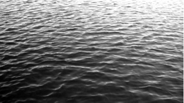
scale map of effective spatial scales	scale map of effective temporal scales
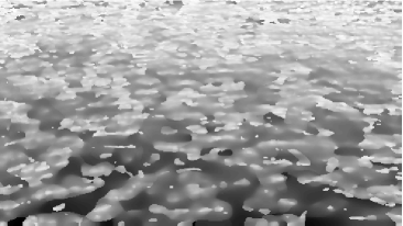
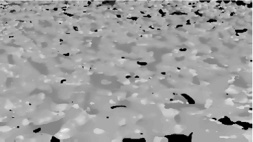
spatio-temporal scale-space signature	maximum magnitude response over all scales

Figure 8: Results of dense spatio-temporal scale selection applied to a video sequence with water waves. The results have been computed with a time-causal and time-recursive spatio-temporal scale-space representation obtained by convolution with a Gaussian kernel over the spatial domain and the time-causal limit kernel over the temporal domain. (top left) Grey-level image. (top right) The spatio-temporal quasi quadrature measure computed at a fixed spatio-temporal scale. (middle left) Selected spatial scale levels in units of effective scale $s_{eff}=\log_{2}\sigma_{s}$. (middle right) Selected temporal scale levels in units of effective scale $\tau_{eff}=\log_{2}\sigma_{\tau}$. (bottom left) Spatio-temporal scale-space signature showing the magnitude variations of the spatio-temporal quasi quadrature measure over both spatial and temporal scales, with effective spatial scale increasing linearly from left to right and effective temporal scale increasing linearly from bottom to top. While this illustration shows the average over all the image points at the given image frame for the purpose of suppressing the influence of local spatial variations, the general dense scale selection method is otherwise local, based on individual scale-space signatures at every image point and for every time moment. (bottom right) The maximum magnitude response over all spatial and temporal scales at every image point. Note from the maps of the selected spatial and temporal scales that there is a clear vertical size gradient for the the selected spatial scales, whereas there is no size gradient for the selected temporal scales. The reason for this is that there are size variations over the spatial domain because of perspective depth effects affecting the spatial scales, whereas the temporal scales are stationary over the image domain, since temporal scale levels are not affected by the perspective mapping. Note that the contrast of the maps showing magnitude information has been set so that dark corresponds to larger values and bright to lower values. In addition, the magnitude maps have been stretched by a square root function. (Results computed using 24 logarithmically distributed spatial scale levels between $\sigma_{s,min}=0.25$ pixels and $\sigma_{s,max}=24$ pixels and 9 logarithmically distributed temporal scale levels between $\sigma_{\tau,min}=10$ ms and $\sigma_{\tau,max}=2.56$ seconds for $C_{s}=1/\sqrt{(1-\Gamma_{s})(2-\Gamma_{s})}$ and $C_{\tau}=1/\sqrt{(1-\Gamma_{\tau})(2-\Gamma_{\tau})}$ using complementary scale normalization parameters $\Gamma_{s}=0$ and $\Gamma_{\tau}=0$.) (Image size: $480\times 270$ pixels. Frame 100 of 250 frames at 25 frames per second.)

grey-level frame	quasi quadrature measure at fixed s-t scale
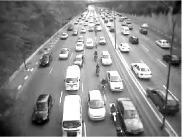
scale map of effective spatial scales	scale map of effective temporal scales
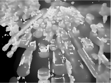
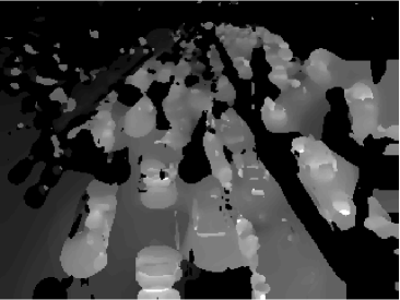
spatio-temporal scale-space signature	maximum magnitude response over all scales

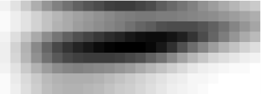
Figure 9: Results of dense spatio-temporal scale selection applied to a traffic scene (video “smooth_traffic05” from the Maryland dynamic scene dataset [57]). Note that distinct responses in the spatial and temporal scale maps are obtained for the different moving cars, again with a size gradient in the spatial scale estimates reflecting the perspective scaling effects, whereas the temporal scale estimates are essentially unaffected by the perspective transformation. Additionally, we can observe that large spatial scales and long temporal scales are selected in the smooth stationary regions on the road and in some parts of the background (Image size: $320\times 240$ pixels. Frame 80 of 1217 frames at 30 frames per second.)

grey-level frame	quasi quadrature measure at fixed s-t scale
scale map of effective spatial scales	scale map of effective temporal scales
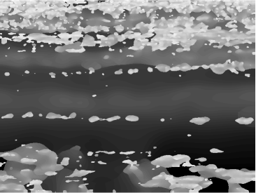
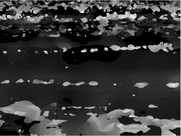
spatio-temporal scale-space signature	maximum magnitude response over all scales

Figure 10: Results of dense spatio-temporal scale selection applied to a scene with breaking waves (from the DynTex dataset [54]). Notice how horizontal stripes of finer spatial and temporal scales are selected at the breaking waves. Notice additionally that there are two dominant spatio-temporal scales in the scene — one for the larger scale overall waves and one for fine-scale spatio-temporal structures where the waves break. (Image size: $768\times 576$ pixels. Frame 50 of 250 frames at 30 frames per second.)

Figure 8 shows an example of applying dense spatio-temporal scale selection to a real video sequence. For reasons of computational efficiency, we only show results obtained using a time-causal and time-recursive spatio-temporal scale-space representation obtained by convolution with Gaussian kernels over the spatial domain and convolution with the time-causal limit kernel over the temporal domain. Because of the time-recursive implementation of this scale-space concept, it is not necessary to explicitly compute and build the five-dimensional spatio-temporal scale-space representation over space-time $(x,y,t)$ and spatio-temporal scales $(s,\tau)$. Instead, the time-recursive implementation builds a four-dimensional representation over the spatial domain $(x,y)$ and the spatio-temporal scale parameters $(s,\tau)$ at every temporal image frame $t$. Then, this representation is recursively updated to the next frame, using only the temporal scale-space representation at the previous frame as a sufficient temporal buffer of past information, using the methodology of time-causal and time-recursive spatio-temporal receptive fields developed in [43].

Because the notion of phase compensation is not yet fully developed for the time-causal limit kernel, we did not use local phase compensation in this experiment. Instead, we restricted ourselves to spatial post-smoothing noting that the approach can in a straightforward manner be extended to temporal post-smoothing by adding a second stage of recursive temporal smoothing to the quasi quadrature measures computed at every image frame. To make the magnitude maps maximally scale invariant for purposes of visualization, we used $\Gamma_{s}=\Gamma_{\tau}=0$.

At every image frame, we computed a discrete approximation of the spatio-temporal quasi quadrature measure at all spatial and temporal scales and detected two-dimensional local extrema over spatial and temporal scales as candidates for local spatio-temporal scale levels. These local extrema were then interpolated to higher resolution over spatial and temporal scales using parabolic interpolation according to [46, Equation (115)]. For simplicity, the results shown in the figures display only the global extremum over spatio-temporal scales at every image point. When applying the scale selection methodology in practice, multiple local extrema over spatio-temporal scales should, however, instead be considered to make it possible to handle multiple characteristic spatio-temporal scale levels at any image point.

From the scale maps in the middle row, we can note that the selected spatial scale levels well reflect the perspective size gradient over the vertical direction in the image domain, caused by the water waves being assumed to have a stationary distribution of wavelengths over the water surface, while these spatial lengths are shortened because of the perspective scaling and foreshortening effects. For the selected temporal scale levels, the distribution is more stationary over the image domain, which can be understood from the assumption that the temporal wavelengths of the waves should be stationary over the water surface, while at the same time the temporal scales are not affected by the perspective transformation (the temporal periodicity of a wave remains the same under imaging transformations).

In the spatio-temporal scale-space signature, showing the average over all the image points of the scale-normalized spatio-temporal quasi quadrature measure as function of the spatial and temporal scales, we can see that for this video sequence there is a narrow range of dominant spatial and temporal scales. The spread over the spatial scale levels is, however, wider than the spread over the temporal scales, caused by the additional variabilities induced by the perspective scaling and foreshortening effects.

When comparing the maximum magnitude response over all spatio-temporal scales to the quasi quadrature measure at a fixed spatio-temporal scale, we can observe that the variability in the maximum over all spatio-temporal scales is lower than the variability in the response at a fixed scale.

Figures 9–10 show results of applying corresponding dense spatio-temporal scale selection to videos of other dynamic scenes. In the traffic scene in figure 9, we can note that distinct responses in the spatial and temporal scale maps are obtained for the different moving cars, again with a vertical size gradient in the spatial scale estimates reflecting the perspective scaling and foreshortening effects, whereas the temporal scale estimates are essentially unaffected by the perspective transformation. Additionally, we can observe that large spatial scales and long temporal scales are selected in the smooth stationary regions on the road and in some parts of the background. For the video of breaking waves in Figure 10, we can note that there are two dominant spatio-temporal scales in the scene — one for the larger scale overall waves and one for fine-scale spatio-temporal structures where the waves break. These two spatio-temporal scale levels are in turn reflected as horizontal stripes in the maps of the selected spatial and temporal scales.

5 Summary and discussion

We have presented a general methodology for performing dense scale selection by detecting local extrema over scale of scale-normalised quasi quadrature entities, which constitute local energy measures of the combined strength of first- and second-order scale-space derivatives. Specifically, we have: (i) analyzed how local scale estimates may in general be strongly dependent on the relative strengths of first- vs. second-order image information at every image point and (ii) proposed two mechanisms to reduce this phase dependency substantially, using post-smoothing and pointwise phase compensation.

Based on the presented theoretical analysis of scale selection properties over a purely spatial image domain, we have in Section 2 presented four types of algorithms for dense scale selection, depending on whether the mechanisms of phase compensation and post-smoothing are included or excluded. For Algorithms II–IV that involve such mechanisms, we have shown that these mechanisms substantially reduce the spatial variability of the local scale estimates compared to the baseline Algorithm I that neither makes use of phase compensation nor post-smoothing. These four methods do all lead to provable scale invariance in the sense that the local scale estimates perfectly follow scaling transformations over image space, and so do image features and image descriptors that are computed at scales proportional to these local scale estimates.

In Section 3, we developed corresponding dense scale selection mechanisms over a purely temporal domain and with corresponding mechanisms of post-smoothing and local phase compensation to reduce the phase sensitivity of the local scale estimates. By experiments on a synthetic sine wave with exponentially varying wavelength as function of time, we demonstrated that the local scale estimates do well adapt to the variabilities of the time-dependent characteristic temporal scales in the signal. By experiments on a neurophysiological signal with approximate stationarity properties, we demonstrated how the proposed dense scale selection methodology is able to reflect multiple levels of characteristic scales in the signal that are not as visible in a spectral analysis based on Fourier transforms.

In Section 4, we combined the above dense scale selection mechanisms over spatial and temporal domains to joint dense spatio-temporal scale selection in video data and demonstrated how the resulting approach is able to generate hypotheses about joint characteristic spatio-temporal scales for different types of dynamic scenes.

A common property of these spatial, temporal and spatio-temporal scale selection methods is that the scale estimates are computed in a bottom-up way from the data in such a way that the scale estimates will be covariant under independent scaling transformations of the spatial and the temporal domains. We propose these forms of dense scale selection as a general mechanisms for estimating local spatial and temporal scales in spatial images, temporal signals and spatio-temporal video.

As a complement to previous scale selection methodologies, which have been primarily applied sparsely at spatial or spatio-temporal interest points, the proposed dense scale selection methodology is intended for applications where spatial, temporal or spatio-temporal receptive field responses are to be computed densely at every image point and for every time moment. Potential applications of such dense receptive field responses include texture analysis over a static spatial domain and dynamic texture analysis over a spatio-temporal domain. For example, if the application of dense spatio-temporal scale selection presented in Figure 8 is applied to videos of water waves taken under different wind conditions, then the spatial scale estimates will reflect the spatial extent of the water waves, whereas the temporal scale estimates will reflect their temporal duration. In this way, dynamic parameters of the water waves can be estimated directly, without using a generative physical model of the wave patterns.

More generally, the proposed framework provides a theory for modelling and measuring how dense receptive field measurements respond selectively at different spatial and temporal scales. This theory should be relevant for a large sets of computer vision problems where receptive field based image measurements in terms of spatial or spatio-temporal $N$-jets are used as the basis for image analysis or video analysis applications. The presented theory could also be relevant for computational modelling of biological vision. If we regard the spatio-temporal quasi quadrature measure (73) as modelling important properties of complex cells as detailed in Section 4.2, then the proposed dense spatio-temporal scale selection theory can explain how complex cells having receptive fields over different ranges of spatial and temporal scales respond selectively to stimuli of different spatial extent and temporal duration.

The only free parameters are the complementary spatial and temporal scale normalization parameters $\Gamma_{s}$ and $\Gamma_{\tau}$, the relative integration scales $c$ for optional post-smoothing and the scale calibration factor by which the generated scale estimates are proportional to the scales at which the local extrema over scales are assumed. These parameters should be optimized to the specific application domain, where the scale dense scale selection methodology is to be combined with higher-level visual modules.

If suitable values of these parameters can be determined for a specific application domain, then by the general scale covariance property of the scale estimates, the proposed dense scale selection theory guarantees that the resulting spatial, temporal or spatio-temporal scale estimates will automatically adapt to and follow variabilities in the characteristic scales in the input images, signals, videos or image streams. In this way, the resulting chain of computer vision/image analysis/signal analysis/video analysis operations can be made provably scale invariant.

Appendix A Detailed analysis of scale calibration for dense spatial scale selection and when using spatial post-smoothing

In the treatment of dense spatial scale selection in Section 2 in the main article, we analysed the scale selection properties obtained from detecting local extrema over scale of the scale-normalized spatial quasi quadrature measure (8)

(90) $$\begin{split}{\cal Q}_{(x,y),\Gamma-norm}L&=\frac{s\,(L_{x}^{2}+L_{y}^{2})+C_{s}\,s^{2}\,(L_{xx}^{2}+2L_{xy}^{2}+L_{yy}^{2})}{s^{\Gamma_{s}}}\end{split}$$

in Section 2.2. Specifically, for the case of using only phase compensation while no post-smoothing to reduce the phase dependency of the spatial scale estimates, the spatial scale estimates are for a 1-D sine wave with angular frequency $\omega_{0}$ centered around the spatial scale level (30)

(91) $$\hat{s}=\sqrt{\hat{s}_{1}\,\hat{s}_{2}}=\frac{\sqrt{(1-\Gamma_{s})(2-\Gamma_{s})}}{\omega_{0}^{2}}$$

By the notion of scale calibration described in Section 2.4, it was proposed that these scale estimates can be calibrated by multiplication with a uniform scale calibration factor to be either:

• equal to the scale estimate $\hat{s}=s_{0}$ obtained by applying the regular scale normalized Laplacian $\nabla_{norm}^{2}L=s\,(L_{xx}+L_{yy})$ or the scale-normalized determinant of the Hessian $\det{\cal H}_{norm}L=s^{2}\,(L_{xx}L_{yy}-L_{xy}^{2})$ at the center of a Gaussian blob of any spatial extent $s_{0}$.

• equal to the scale estimate $\hat{s}=\sqrt{2}/\omega_{0}^{2}$ corresponding to the geometric average of the scale estimates obtained for a sine wave of any angular frequency $\omega_{0}$ when $\Gamma_{s}=0$.

In this appendix section, we describe in more detail how such scale calibration can be performed when also using spatial post-smoothing.

A.1 Influence of the post-smoothing scale

When applying post-smoothing, the variability in the spatial scale estimates decreases with the relative integration scale parameter $c$ (see the third, fourth and fifth rows in Figure 3). The minimum scale estimates are assumed at the spatial points at which ${\cal Q}_{(x,y),\Gamma-norm}L$ only responds to first-order information, whereas the maximum scale estimates are assumed at the points at which ${\cal Q}_{(x,y),\Gamma-norm}L$ only responds to second-order information.

By differentiating the 1-D version of (LABEL:eq-Qnormbar-2D-sine-wave-general) with respect to scale $s$ and setting $x=0$ and $x=\omega_{0}\pi/2$ respectively as well as $\omega_{0}=1$ in the resulting equation, we obtain the following algebraic equations for how the minimum and maximum scale values depend on the relative post-smoothing scale $c$, $\Gamma_{s}$ and $C_{s}$ for a 1-D sine wave with angular frequency $\omega_{0}$:

$$\begin{split}C_{s}\left(2c^{2}+1\right)s^{2}-e^{2c^{2}s}\left(C_{s}s^{2}-2C_{s}s+C_{s}s\Gamma_{s}+s-1+\Gamma_{s}\right)\end{split}$$

(92) $$\begin{split}\quad-s\left(2C_{s}+2c^{2}+1\right)+\Gamma_{s}(C_{s}s-1)+1=0,\end{split}$$

$$\begin{split}C_{s}-2C_{s}c^{2}s^{2}-e^{2c^{2}s}\left(C_{s}s^{2}-2C_{s}s+C_{s}s\Gamma_{s}+s-1+\Gamma_{s}\right)\end{split}$$

(93) $$\begin{split}\quad-C_{s}s^{2}+2C_{s}s-C_{s}s\Gamma_{s}+2c^{2}s+s-1+\Gamma_{s}=0.\end{split}$$

By defining functions $S_{sine,1}(\Gamma_{s},c,C_{s})$ and $S_{sine,1}(\Gamma_{s},c,C_{s})$ that represent the solutions $\hat{s}_{min}$ and $\hat{s}_{max}$ of these equations as function of the parameters $\Gamma_{s}$, $c$ and $C_{s}$ for $\omega_{0}=1$, the minimum and maximum scale values can because of the self-similarity over scale for an arbitrary angular frequency $\omega_{0}$ of the sine wave be expressed as:

(94) $$\hat{s}_{min}=\frac{S_{sine,1}(\Gamma_{s},c,C_{s})}{\omega_{0}^{2}},\quad\quad\hat{s}_{max}=\frac{S_{sine,2}(\Gamma_{s},c,C_{s})}{\omega_{0}^{2}}.$$

Table 2 shows numerical values of these entities for different values of the scale normalization parameter $\Gamma_{s}$ and the relative post-smoothing scale $c$.

Minimum relative scale estimate $\hat{s}_{min}=S_{sine,1}(\Gamma_{s},c,C_{s})$ for a 1-D sine wave

$c$	$\Gamma_{s}=0$	$\Gamma_{s}=\frac{1}{4}$	$\Gamma_{s}=\frac{1}{2}$
0	1.000	0.750	0.500
$1/2$	1.033	0.741	0.466
$1/\sqrt{2}$	1.132	0.772	0.446
1	1.329	0.963	0.451
$\sqrt{2}$	1.408	1.125	0.779
$2$	1.414	1.145	0.863

Maximum relative scale estimate $\hat{s}_{min}=S_{sine,2}(\Gamma_{s},c,C_{s})$ for 1-D sine wave

$c$	$\Gamma_{s}=0$	$\Gamma_{s}=\frac{1}{4}$	$\Gamma_{s}=\frac{1}{2}$
0	2.000	1.750	1.500
$1/2$	1.701	1.485	1.264
$1/\sqrt{2}$	1.584	1.363	1.147
1	1.474	1.242	1.021
$\sqrt{2}$	1.420	1.163	0.914
$2$	1.414	1.146	0.869

Table 2: Minimum and maximum scale estimates $\hat{s}_{min}=S_{sine,1}(\Gamma_{s},c,C_{s})/\omega_{0}^{2}$ and $\hat{s}_{max}=S_{sine,2}(\Gamma_{s},c,C_{s})/\omega_{0}^{2}$ for dense scale selection based on local extrema over scale of the post-smoothed quasi quadrature entity ${\overline{\cal Q}}_{(x,y),\Gamma-norm}L$ applied to a 1-D sine wave with angular frequency $\omega_{0}=1$ for different values of the relative scale normalization parameter $\Gamma_{s}$ and the relative post-smoothing scale $c$ with $C_{s}$ according to (25). These entities are defined as the solutions of equations (A.1) and (A.1), and for increasing values of $c$ they approach $\hat{s}_{intermed}=\sqrt{(1-\Gamma_{s})\,(2-\Gamma_{s})}/\omega_{0}^{2}$ in (24).

Whereas the functions $S_{sine,1}(\Gamma_{s},c,C_{s})$ and $S_{sine,1}(\Gamma_{s},c,C_{s})$ are not expressed in terms of elementary functions, it is straightforward to implement these functions using standard numerical methods for computing the solutions of a 1-D equation.

A.2 Phase-compensated scale estimates with post-smoothing

Given these expressions for the minimum and maximum scale estimates for a sine wave, we can also define a corresponding notion of phase compensation in the presence of spatial post-smoothing:

$$\begin{split}\hat{s}_{{\overline{\cal Q}}L,comp}=&\frac{\sqrt{S_{sine,1}(\Gamma_{s},c,C_{s})\,S_{sine,2}(\Gamma_{s},c,C_{s})}}{\left(\overline{\cal Q}_{(x,y),1,\Gamma-norm}L+\overline{\cal Q}_{(x,y),2,\Gamma-norm}L\right)}\times\end{split}$$

(95) $$\begin{split}&\left(\frac{\overline{\cal Q}_{(x,y),1,\Gamma-norm}L}{S_{sine,1}(\Gamma_{s},c,C_{s})}+\frac{\overline{\cal Q}_{(x,y),2,\Gamma-norm}L}{S_{sine,2}(\Gamma_{s},c,C_{s})}\right)\,\hat{s}_{{\overline{\cal Q}}L}\end{split}$$

or

$$\begin{split}&\hat{s}_{{\cal Q}L,comp}=\sqrt{S_{sine,1}(\Gamma_{s},c,C_{s})\,S_{sine,2}(\Gamma_{s},c,C_{s})}\,\hat{s}_{{\cal Q}L}/\end{split}$$

$$\begin{split}(S_{sine,1}(\Gamma_{s},c,C_{s}))^{\frac{\overline{\cal Q}_{(x,y),1,\Gamma-norm}L}{\overline{\cal Q}_{(x,y),1,\Gamma-norm}L+\overline{\cal Q}_{(x,y),2,\Gamma-norm}L}}/\end{split}$$

(96) $$\begin{split}(S_{sine,2}(\Gamma_{s},c,C_{s}))^{\frac{\overline{\cal Q}_{(x,y),2,\Gamma-norm}L}{\overline{\cal Q}_{(x,y),1,\Gamma-norm}L+\overline{\cal Q}_{(x,y),2,\Gamma-norm}L}}\end{split}$$

with $\overline{\cal Q}_{(x,y),1,\Gamma-norm}L$ and $\overline{\cal Q}_{(x,y),2,\Gamma-norm}L$ according to (12) and (13) and with the normalization chosen such that the scale values should aim towards the geometric mean of the extreme values $S_{sine,1}(\Gamma_{s},c,C_{s})$ and $S_{sine,2}(\Gamma_{s},c,C_{s})$ according to (A.1) and (A.1).

A.2.1 Two-dimensional blob

For a two-dimensional Gaussian blob

(97) $$f(x,y)=g(x,y;\;s_{0})=\frac{1}{2\pi s_{0}}e^{-(x^{2}+y^{2})/2s_{0}},$$

if follows from the semi-group property of the Gaussian that the scale-space representation is given by

(98) $$L(x,y;\;s)=g(x,y;\;s_{0}+s)=\frac{1}{2\pi(s_{0}+s)}e^{-(x^{2}+y^{2})/2(s_{0}+s)}$$

and the unsmoothed quasi quadrature entity at the origin is of the form

(99) $${\cal Q}_{(x,y),\Gamma-norm}L=\frac{C_{s}s^{2-\Gamma_{s}}}{2\pi^{2}(s+s_{0})^{4}}.$$

Differentiating this expression with respect to the scale parameter $s$, shows that the maximum value over scales is assumed at scale

(100) $$\hat{s}_{Gauss}=\frac{2-\Gamma_{s}}{2+\Gamma_{s}}\,s_{0}.$$

With complementary post-smoothing with relative integration scale $c$, corresponding computation of the post-smoothed quasi quadrature and differentiation of the resulting expression gives an algebraic equation of the form

$$\begin{split}4c^{6}s^{2}\left((2C_{s}+1)s^{2}(2+\Gamma_{s})\right.\left.+2ss_{0}(C_{s}(\Gamma_{s}-1)+1+\Gamma_{s})+s_{0}^{2}\Gamma_{s}\right)+\end{split}$$

$$\begin{split}+4c^{4}s(s+s_{0})\left((2C_{s}+1)s^{2}(2+\Gamma_{s})\right.\left.+ss_{0}(2C_{s}(\Gamma_{s}-2)+1+2\Gamma_{s})+s_{0}^{2}(\Gamma_{s}-1)\right)+\end{split}$$

$$\begin{split}+c^{2}(s+s_{0})^{2}\left((4C_{s}+1)s^{2}(2+\Gamma_{s})\right.\left.+2ss_{0}(2C_{s}(\Gamma_{s}-1)+\Gamma_{s})+s_{0}^{2}(\Gamma_{s}-2)\right)\end{split}$$

(101) $$\begin{split}+C_{s}(s+s_{0})^{3}(s(2+\Gamma_{s})+s_{0}(\Gamma_{s}-2))=0\end{split}$$

for the selected scale level $\hat{s}$ as function of the complementary scale normalization parameter $\Gamma_{s}$, the relative post-smoothing scale $c$ and the relative weighting factor $C_{s}$ between first- and second-order information. Let us define the following function for representing the solution of this equation:

(102) $$\hat{s}=S_{Gauss}(\Gamma_{s},c,C_{s})\,s_{0}.$$

Table 3 shows numerical values of this entity for different values of $\Gamma_{s}$ and $c$.

Scale estimates $\hat{s}=S_{Gauss}(\Gamma_{s},c)\,s_{0}$ based on $\overline{\cal Q}_{(x,y),\Gamma-norm}L$
at the center of a Gaussian blob

$c$	$\Gamma_{s}=0$	$\Gamma_{s}=\frac{1}{4}$	$\Gamma_{s}=\frac{1}{2}$
0	1.000	0.778	0.600
$1/2$	0.839	0.650	0.498
$1/\sqrt{2}$	0.751	0.578	0.440
1	0.641	0.487	0.367
$\sqrt{2}$	0.519	0.385	0.283
$2$	0.402	0.285	0.199

Table 3: Numerical values of the ratio $\hat{s}/s_{0}=S_{Gauss}(\Gamma_{s},c,C_{s})$ for which the post-smoothed quasi quadrature entity $\overline{\cal Q}_{(x,y),\Gamma-norm}L$ assumes its maximum over scale at the center of a Gaussian blob with scale parameter $s_{0}$ for different values of the complementary scale normalization parameter $\Gamma_{s}$ and the relative post-smoothing scale parameter $c$ with $C_{s}$ according to (25).

The difference in net effect between the Gaussian scale calibration model and the sine wave scale calibration model under variations of $\Gamma_{s}$ and $c$ is essentially determined by the variation of the following ratio between the scale calibration factors in units of $\sigma_{s}=\sqrt{s}$:

(103) $$\chi(\Gamma_{s},c)=\sqrt{\frac{2S_{Gauss}(\Gamma_{s},c)}{S_{sine,2}(\Gamma_{s},c)}}$$

see Table 4 for numerical values. For $c\leq 1$, it can be seen that the relative differences in effects for scale calibration are within a range of 15 % in units of $\sigma_{s}=\sqrt{s}$.

Given the similarity between the results obtained from these qualitatively very different models, it seems plausible that the results should also generalize to wider classes of image structures. Choosing the parameter $\gamma$ for scale selection using $\gamma$-normalized derivatives based on the behaviour for Gaussian image models has also been demonstrated to lead to highly useful results for a wide range of computer vision tasks (Lindeberg [35, 34, 37, 41]).

Dependency of the ratio between the scale calibration factors $\sqrt{\frac{2S_{Gauss}(\Gamma_{s},c)}{S_{sine,2}(\Gamma_{s},c)}}$ on $\Gamma_{s}$ and $c$

$c$	$\Gamma_{s}=0$	$\Gamma_{s}=\frac{1}{4}$	$\Gamma_{s}=\frac{1}{2}$
0	1.000	0.943	0.894
$1/2$	0.991	0.935	0.888
$1/\sqrt{2}$	0.974	0.921	0.876
1	0.933	0.886	0.848
$\sqrt{2}$	0.855	0.814	0.786
$2$	0.754	0.705	0.677

Table 4: Numerical values of the ratio between the scale calibration factors $S_{Gauss}(\Gamma_{s},c)$ and $S_{sine,2}(\Gamma_{s},c)$ in units of $\sigma_{s}=\sqrt{s}$ and normalized such that the ratio is equal to one for $\Gamma_{s}=0$ and $c=0$. This ratio provides an estimate of how much the calibrated scale estimates will depend on the choice of calibration model, based on either sparse image features or a dense texture pattern.

Appendix B Detailed analysis of phase compensation and scale calibration for dense spatio-temporal scale selection

For dense spatio-temporal scale selection, we do according to Section 4 at every point $(x,y,t)$ in space-time detect simultaneous local extrema over spatio-temporal scales (81)

(104) $$(\hat{s}_{{\cal Q}_{(x,y,t),\Gamma-norm}},\hat{\tau}_{{\cal Q}_{(x,y,t),\Gamma-norm}})=\operatorname{argmaxlocal}_{s,\tau}{\cal Q}_{(x,y,t),\Gamma-norm}L$$

of the scale-normalized spatio-temporal quasi quadrature entity (73)

$$\begin{split}&{\cal Q}_{(x,y,t),\Gamma-norm}L\end{split}$$

$$\begin{split}&=\frac{\tau\,{\cal Q}_{(x,y),\Gamma-norm}L_{t}+C_{\tau}\tau^{2}\,{\cal Q}_{(x,y),\Gamma-norm}L_{tt}}{\tau^{\Gamma_{\tau}}}\end{split}$$

$$\begin{split}&=\frac{1}{s^{\Gamma_{s}}\tau^{\Gamma_{\tau}}}\left(\tau\left(s\,(L_{xt}^{2}+L_{yt}^{2})+C_{s}\,s^{2}\left(L_{xxt}^{2}+2L_{xyt}^{2}+L_{yyt}^{2}\right)\right)\right.\end{split}$$

(105) $$\begin{split}&\phantom{=\frac{1}{s^{\Gamma_{s}}\tau^{\Gamma_{\tau}}}\left(\right.}\,\left.+C_{\tau}\,\tau^{2}\left(s\,(L_{xtt}^{2}+L_{ytt}^{2})+C_{s}\,s^{2}(L_{xxtt}^{2}+2L_{xytt}^{2}+L_{yytt}^{2})\right)\right).\end{split}$$

regular scale estimates $\Gamma_{s}=\Gamma_{\tau}=0$	phase-compensated $\Gamma_{s}=\Gamma_{\tau}=0$
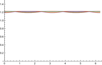
regular scale estimates $\Gamma_{s}=\Gamma_{\tau}=1/4$	phase-compensated $\Gamma_{s}=\Gamma_{\tau}=1/4$
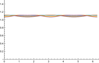
regular scale estimates $\Gamma_{s}=\Gamma_{\tau}=1/2$	phase-compensated $\Gamma_{s}=\Gamma_{\tau}=1/2$

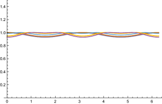
Figure 11: Spatial variability of spatial scale estimates $\hat{\sigma}_{s}=\sqrt{s}$ computed (left column) from local extrema over spatial scale of the $\Gamma$-normalized quasi quadrature measure ${\cal Q}_{(x,y,t),\Gamma-norm}L$ according to (81) for a 2+1-D spatio-temporal sine wave with spatial angular frequency $\omega_{s}=1$ and (right column) with phase compensation of the scale estimates according to (LABEL:eq-Q3-spat-scaleest-phasecorr-geom-sine-s). (Horizontal axis: spatial position $t$) (The multiple graphs in each diagram show the variability of the scale estimates for different values of the complementary spatial coordinate $y=n\pi/8$.)

regular scale estimates $\Gamma_{s}=\Gamma_{\tau}=0$	phase-compensated $\Gamma_{s}=\Gamma_{\tau}=0$
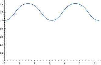
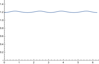
regular scale estimates $\Gamma_{s}=\Gamma_{\tau}=1/4$	phase-compensated $\Gamma_{s}=\Gamma_{\tau}=1/4$
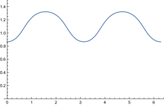
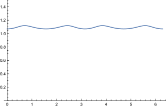
regular scale estimates $\Gamma_{s}=\Gamma_{\tau}=1/2$	phase-compensated $\Gamma_{s}=\Gamma_{\tau}=1/2$

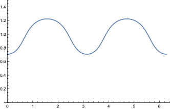
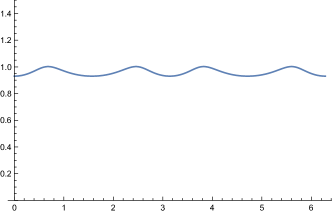
Figure 12: Temporal variability of temporal scale estimates $\hat{\sigma}_{\tau}=\sqrt{\tau}$ computed (left column) from local extrema over temporal scale of the $\Gamma$-normalized quasi quadrature measure ${\cal Q}_{(x,y,t),\Gamma-norm}L$ according to (81) for a 2+1-D spatio-temporal sine wave with spatial angular frequency $\omega_{s}=1$ and (right column) with phase compensation of the scale estimates according to (LABEL:eq-Q3-temp-scaleest-phasecorr-geom-sine-tau). (Horizontal axis: time $t$)

B.1 Phase-compensated scale estimates

Given the understanding from Section 4.3 of how the local spatio-temporal scale estimates depend on the local phase of a sine wave, we can define phase-compensated spatial and temporal scale estimates according to

$$\begin{split}&\hat{s}_{{\cal Q}_{(x,y,t)L,comp}}=\end{split}$$

(106) $$\begin{split}&\frac{\sqrt{(1-\Gamma_{s})(2-\Gamma_{s})}\,\hat{s}_{{\cal Q}_{(x,y,t)L,\Gamma-norm}}}{(1-\Gamma_{s})^{\frac{{\cal Q}_{1,(x,y),\Gamma-norm}L_{t}+C_{\tau}{\cal Q}_{1,(x,y),\Gamma-norm}L_{tt}}{{\cal Q}_{(x,y,t),\Gamma-norm}L}}(2-\Gamma_{s})^{\frac{{\cal Q}_{2,(x,y),\Gamma-norm}L_{t}+C_{\tau}{\cal Q}_{2,(x,y),\Gamma-norm}L_{tt}}{{\cal Q}_{(x,y,t),\Gamma-norm}L}}},\end{split}$$

$$\begin{split}&\hat{\tau}_{{\cal Q}_{(x,y,t)L,comp}}=\end{split}$$

(107) $$\begin{split}&\frac{\sqrt{(1-\Gamma_{\tau})(2-\Gamma_{\tau})}\,\hat{\tau}_{{\cal Q}_{(x,y,t)L,\Gamma-norm}}}{(1-\Gamma_{\tau})^{\frac{{\cal Q}_{1,(x,y),\Gamma-norm}L_{t}+{\cal Q}_{2,(x,y),\Gamma-norm}L_{t}}{{\cal Q}_{(x,y,t),\Gamma-norm}L}}(2-\Gamma_{\tau})^{\frac{C_{\tau}\left({\cal Q}_{1,(x,y),\Gamma-norm}L_{tt}+{\cal Q}_{2,(x,y),\Gamma-norm}L_{tt}\right)}{{\cal Q}_{(x,y,t),\Gamma-norm}L}}},\end{split}$$

defined to be equal to the geometric averages of the extreme values

(108) $$\begin{split}\hat{s}=\sqrt{\hat{s}_{1}\,\hat{s}_{2}}=\frac{\sqrt{(1-\Gamma_{s})(2-\Gamma_{s})}}{\omega_{0}^{2}}\end{split}$$

(109) $$\begin{split}\hat{\tau}=\sqrt{\hat{\tau}_{1}\,\hat{\tau}_{2}}=\frac{\sqrt{(1-\Gamma_{\tau})(2-\Gamma_{\tau})}}{\omega_{\tau}^{2}}\end{split}$$

in the extreme cases when only one of the first- or second-order components in the components responds and with a much lower variability in between because of the blending of the responses to the first- vs. second-order spatial or temporal derivatives (see figures 11–12).

From these spatial and temporal scale estimates, we can in turn estimate the spatial and temporal wavelengths of the sine wave according to

(110) $$\begin{split}\hat{\lambda}_{s}&=\frac{2\pi\sqrt{\hat{s}_{{\cal Q}_{(x,y,t)L,comp}}}}{\sqrt[4]{(1-\Gamma_{s})(2-\Gamma_{s})}},\end{split}$$

(111) $$\begin{split}\hat{\lambda}_{\tau}&=\frac{2\pi\sqrt{\hat{\tau}_{{\cal Q}_{(x,y,t)L,comp}}}}{\sqrt[4]{(1-\Gamma_{\tau})(2-\Gamma_{\tau})}}.\end{split}$$

B.2 Scale calibration

When applied to a Gaussian blink of spatial extent $s_{0}$ and temporal duration $\tau_{0}$

(112) $$f(x,y,t)=g(x,y;\;s_{0})\,g(t;\;\tau_{0})=\frac{1}{(2\pi)^{3/2}s_{0}\sqrt{\tau_{0}}}\,e^{-(x^{2}+y^{2})/2s_{0}}\,e^{-t^{2}/2\tau_{0}},$$

for which the spatio-temporal scale-space representation is of the form

(113) $$L(x,y,t;\;s_{0},\tau_{0})=g(x,y;\;s_{0}+s)\,g(t;\;\tau_{0}+\tau),$$

the spatial and temporal scale estimates will according to the theoretical analysis in (Lindeberg [44, 45]) be given by

(114) $$\begin{split}\hat{s}&=\frac{\gamma_{s}s_{0}}{2-\gamma_{s}}\,s_{0},\end{split}$$

(115) $$\begin{split}\hat{\tau}&=\frac{2\gamma_{\tau}\tau_{0}}{3-2\gamma_{\tau}}\,\tau_{0}.\end{split}$$

Here, for $\gamma_{s}=1-\Gamma_{s}/2$ and $\gamma_{\tau}=1-\Gamma_{\tau}/2$ this implies that the regular scale estimates for a Gaussian blink are

(116) $$\begin{split}\hat{s}&=\frac{2-\Gamma_{s}}{2+\Gamma_{s}}\,s_{0},\end{split}$$

(117) $$\begin{split}\hat{\tau}&=\frac{2-\Gamma_{\tau}}{1+\Gamma_{\tau}}\,\tau_{0},\end{split}$$

and the corresponding phase-compensated scale estimates

(118) $$\begin{split}\hat{s}_{{\cal Q}_{(x,y,t)L,comp}}=\frac{\sqrt{(2-\Gamma_{s})(1-\Gamma_{s})}}{2+\Gamma_{s}}\,s_{0},\end{split}$$

(119) $$\begin{split}\hat{\tau}_{{\cal Q}_{(x,y,t)L,comp}}=\frac{\sqrt{(2-\Gamma)(1-\Gamma)}}{1+\Gamma_{\tau}}\,\tau_{0}.\end{split}$$

If we want to calibrate the spatial and temporal scale estimates such that the spatial and temporal scale estimates are equal to $\hat{s}=s_{0}$ and $\hat{\tau}=\tau_{0}$ for a Gaussian blink of spatial extent $s_{0}$ and temporal duration $\tau_{0}$, we should therefore calibrate the phase compensated scale estimates $\hat{s}_{{\cal Q}_{(x,y,t)L,comp}}$ and $\hat{\tau}_{{\cal Q}_{(x,y,t)L,comp}}$ according to

(120) $$\begin{split}\hat{s}_{{\cal Q}_{(x,y,t)L,calib}}=\frac{2+\Gamma_{s}}{\sqrt{(2-\Gamma_{s})(1-\Gamma_{s})}}\,\hat{s}_{{\cal Q}_{(x,y,t)L,comp}},\end{split}$$

(121) $$\begin{split}\hat{\tau}_{{\cal Q}_{(x,y,t)L,calib}}=\frac{1+\Gamma_{\tau}}{\sqrt{(2-\Gamma_{\tau})(1-\Gamma_{\tau})}}\,\hat{\tau}_{{\cal Q}_{(x,y,t)L,comp}}.\end{split}$$

With this scale calibration, since the scale estimate for a Gaussian temporal onset ramp, which for regular $\gamma$-normalized temporal derivatives assumes the form (Lindeberg [34, equation (23)])

(122) $$\hat{s}=\frac{\gamma}{1-\gamma}\,s_{0}=\left\{\gamma=1-\Gamma\right\}=\frac{1-\Gamma}{\Gamma}\,s_{0},$$

the spatial scale estimate for a diffuse Gaussian edge will by combination of (LABEL:eq-Q3-spat-scaleest-phasecorr-geom-sine-s) with (120) be given by

(123) $$\hat{s}=\frac{2+\Gamma_{s}}{\Gamma_{s}}\,s_{0},$$

whereas the temporal scale estimate for a Gaussian onset ramp will by combination of (LABEL:eq-Q3-temp-scaleest-phasecorr-geom-sine-tau) with (121) be given by

(124) $$\hat{\tau}=\frac{1+\Gamma_{\tau}}{\Gamma_{\tau}}\,\tau_{0}.$$

By varying the parameters $\Gamma_{s}$ and $\Gamma_{\tau}$ we can thereby regulate the factor by which the spatial scale estimate for a diffuse Gaussian edge will be proportional to its diffuseness and in a corresponding manner the factor by which the temporal scale estimate for a Gaussian onset ramp will be proportional to its temporal duration, while ensuring that the spatial and temporal scale estimates for a Gaussian blink will still reflect the spatial extent and the temporal duration of the Gaussian blink.

regular magnitudes $\Gamma_{s}=\Gamma_{\tau}=0$	phase-compensated $\Gamma_{s}=\Gamma_{\tau}=0$
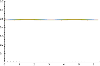
regular magnitudes $\Gamma_{s}=\Gamma_{\tau}=1/4$	phase-compensated $\Gamma_{s}=\Gamma_{\tau}=1/4$
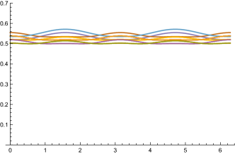
regular magnitudes $\Gamma_{s}=\Gamma_{\tau}=1/2$	phase-compensated $\Gamma_{s}=\Gamma_{\tau}=1/2$

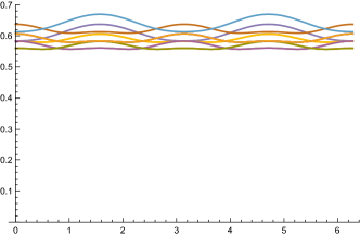
Figure 13: Spatial variability of magnitude responses ${\cal Q}_{(x,y,t),\Gamma-norm}$ computed (left column) at the local extrema over both spatial and temporal scales of the $\Gamma$-normalized quasi quadrature measure ${\cal Q}_{(x,y,t),\Gamma-norm}$ according to (81) for a 2+1-D spatio-temporal sine wave pattern of spatial angular frequency $\omega_{s}=1$ and temporal angular frequency $\omega_{\tau}=1$ (right column) at phase-compensated scale estimates according to (LABEL:eq-Q3-spat-scaleest-phasecorr-geom-sine-s) and (LABEL:eq-Q3-temp-scaleest-phasecorr-geom-sine-tau). (Horizontal axis: spatial coordinate $x$) (The multiple graphs in each diagram show the variability of the scale estimates for different values of the complementary spatial coordinate $y=m\pi/4$ and the temporal coordinate $t=n\pi/4$.)

regular magnitudes $\Gamma_{s}=\Gamma_{\tau}=0$	phase-compensated $\Gamma_{s}=\Gamma_{\tau}=0$
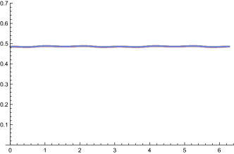
regular magnitudes $\Gamma_{s}=\Gamma_{\tau}=1/4$	phase-compensated $\Gamma_{s}=\Gamma_{\tau}=1/4$
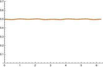
regular magnitudes $\Gamma_{s}=\Gamma_{\tau}=1/2$	phase-compensated $\Gamma_{s}=\Gamma_{\tau}=1/2$

Figure 14: Temporal variability of magnitude responses ${\cal Q}_{(x,y,t),\Gamma-norm}$ computed (left column) at the local extrema over both spatial and temporal scales of the $\Gamma$-normalized quasi quadrature measure ${\cal Q}_{(x,y,t),\Gamma-norm}$ according to (81) for a 2+1-D spatio-temporal sine wave pattern of spatial angular frequency $\omega_{s}=1$ and temporal angular frequency $\omega_{\tau}=1$ (right column) at phase-compensated scale estimates according to (LABEL:eq-Q3-spat-scaleest-phasecorr-geom-sine-s) and (LABEL:eq-Q3-temp-scaleest-phasecorr-geom-sine-tau). (Horizontal axis: time $t$) (The multiple graphs in each diagram show the variability of the scale estimates for different values of the complementary spatial coordinates $x=m\pi/4$ and $y=n\pi/4$.)

B.3 Phase-compensated magnitude estimates

When performing temporal scale selection from the local extrema of the scale-normalized quasi quadrature measure over scale (73), the magnitude responses at the spatial points $(x=n\pi/\omega_{s},y=n\pi/\omega_{s})$ and the temporal moments $t=n\pi/\omega_{\tau}$ at which only the first-order temporal derivative responds are given by

(125) $${\cal Q}_{t,1,\Gamma-norm}=2(1-\Gamma_{s})^{1-\Gamma_{s}}(1-\Gamma_{\tau})^{1-\Gamma_{\tau}}\,e^{\Gamma_{s}+\Gamma_{\tau}-2}\,\omega_{s}^{2\Gamma_{s}}\,\omega_{\tau}^{2\Gamma_{\tau}},$$

whereas the magnitude responses at the spatial points $(x=(\pi/2+n\pi)/\omega_{s},y=(\pi/2+n\pi)/\omega_{s})$ and the temporal moments $t=(\pi/2+n\pi)/\omega_{0}^{2}$ at which only the second-order temporal derivative responds are given by

(126) $${\cal Q}_{t,2,\Gamma-norm}=\frac{2(2-\Gamma_{s})^{2-\Gamma_{s}}(2-\Gamma_{\tau})^{2-\Gamma_{\tau}}\,e^{\Gamma_{s}+\Gamma_{\tau}-4}\,\omega_{s}^{2\Gamma_{s}}\,\omega_{\tau}^{2\Gamma_{\tau}}}{\sqrt{(2-\Gamma_{s})(1-\Gamma_{s})}\sqrt{(2-\Gamma_{\tau})(1-\Gamma_{\tau})}}.$$

Thus, the magnitude responses will have a certain phase dependency because of the variability in the temporal scale estimates leading to corresponding variability in the relative strengths of the first- vs. second-order responses (see the left columns in figures 13–14). When performing phase compensation according to (LABEL:eq-Q3-spat-scaleest-phasecorr-geom-sine-s) and (LABEL:eq-Q3-temp-scaleest-phasecorr-geom-sine-tau), the temporal scale estimates will on the other hand will be close to a temporal scale level where the relative strengths of the first- and second-order responses are balanced and leading to a much lower temporal variability in the magnitude responses (see the right columns in figures 13–14). If one additionally wants these magnitude estimates to be independent of the wavelengths of the sine wave pattern, then this can be accomplished by instead computing the corresponding post-normalized quasi quadrature entity

(127) $${\cal Q}_{(x,y,t),post-norm}=\hat{s}^{\Gamma_{s}}\,\hat{\tau}^{\Gamma_{\tau}}\,{\cal Q}_{(x,y,t),\Gamma-norm}$$

where $\hat{s}$ and $\hat{\tau}$ represent the phase-compensated spatial and temporal scale estimates according to (LABEL:eq-Q3-spat-scaleest-phasecorr-geom-sine-s) and (LABEL:eq-Q3-temp-scaleest-phasecorr-geom-sine-tau).

In these respects, the analysis in this appendix shows how the notion of phase compensation also applies in a spatio-temporal setting with independent variabilities in the spatial and the temporal scales in the spatio-temporal image structures in video data.

When reduced to either a purely spatial or a purely temporal domain, the analysis in this appendix also gives a more detailed treatment of how the notion of scale calibration can be performed when applying dense scale selection to either purely spatial image data or a purely temporal signal. Specifically, the expressions (123) and (124) show how variations in the complementary scale normalization parameters $\Gamma_{s}$ and $\Gamma_{\tau}$ will influence the selection of spatial and temporal scales at diffuse spatial edges and temporal ramps.

References

- [1] A. Almansa and T. Lindeberg, Fingerprint enhancement by shape adaptation of scale-space operators with automatic scale-selection, IEEE Transactions on Image Processing, 9 (2000), pp. 2027–2042.
- [2] H. Bay, A. Ess, T. Tuytelaars, and L. van Gool, Speeded up robust features (SURF), Computer Vision and Image Understanding, 110 (2008), pp. 346–359.
- [3] R. N. Bracewell, The Fourier Transform and its Applications, McGraw-Hill, New York, 1999. 3rd edition.
- [4] L. Bretzner, I. Laptev, and T. Lindeberg, Hand-gesture recognition using multi-scale colour features, hierarchical features and particle filtering, in Proc. Face and Gesture, Washington D.C., USA, May. 2002, pp. 63–74.
- [5] L. Bretzner and T. Lindeberg, Feature tracking with automatic selection of spatial scales, Computer Vision and Image Understanding, 71 (1998), pp. 385–392.
- [6] T. Brox and J. Weickert, A TV flow based local scale estimate and its application to texture discrimination, Journal of Visual Communication and Image Representation, 17 (2006), pp. 1053–1073.
- [7] H. Cagnan, E. P. Duff, and P. Brown, The relative phases of basal ganglia activties dynamically shape effective connectivity in Parkinson’s disease, Brain, 138 (2016), pp. 1667–1678.
- [8] O. Chomat, V. de Verdiere, D. Hall, and J. Crowley, Local scale selection for Gaussian based description techniques, in Proc. European Conf. on Computer Vision (ECCV 2000), vol. 1842 of Springer LNCS, Dublin, Ireland, 2000, pp. I:117–133.
- [9] L. Cohen, Time-frequency analysis, vol. 778, Prentice Hall PTR Englewood Cliffs, NJ:, 1995.
- [10] D. Comaniciu, V. Ramesh, and P. Meer, The variable bandwidth mean shift and data-driven scale selection, in Proc. International Conference on Computer Vision (ICCV 2001), Vancouver, Canada, 2001, pp. 438–445.
- [11] G. C. DeAngelis and A. Anzai, A modern view of the classical receptive field: Linear and non-linear spatio-temporal processing by V1 neurons, in The Visual Neurosciences, L. M. Chalupa and J. S. Werner, eds., vol. 1, MIT Press, 2004, pp. 704–719.
- [12] G. C. DeAngelis, I. Ohzawa, and R. D. Freeman, Receptive field dynamics in the central visual pathways, Trends in Neuroscience, 18 (1995), pp. 451–457.
- [13] C. Dyken and M. S. Floater, Transfinite mean value interpolation, Computer Aided Geometric Design, 26 (2009), pp. 117–134.
- [14] L. M. J. Florack, Image Structure, Series in Mathematical Imaging and Vision, Springer, 1997.
- [15] D. Gabor, Theory of communication, Journal of the IEE, 93 (1946), pp. 429–457.
- [16] L. D. Griffin, The second order local-image-structure solid, IEEE Trans. Pattern Analysis and Machine Intell., 29 (2007), pp. 1355–1366.
- [17] C. Hammond, H. Bergman, and P. Brown, Pathological synchronization in Parkinson’s disease: networks, models and treatment, Trends in Neurosciences, 30 (2007), pp. 357–364.
- [18] T. Hassner, S. Filosof, V. Mayzels, and L. Zelnik-Manor, Sifting through scales, IEEE Transactions on Pattern Analysis and Machine Intelligence, 39 (2017), pp. 1431–1443.
- [19] D. H. Hubel and T. N. Wiesel, Receptive fields of single neurones in the cat’s striate cortex, J Physiol, 147 (1959), pp. 226–238.
- [20] D. H. Hubel and T. N. Wiesel, Receptive fields, binocular interaction and functional architecture in the cat’s visual cortex, J Physiol, 160 (1962), pp. 106–154.
- [21] D. H. Hubel and T. N. Wiesel, Brain and Visual Perception: The Story of a 25-Year Collaboration, Oxford University Press, 2005.
- [22] T. Iijima, Basic theory on normalization of pattern (in case of typical one-dimensional pattern), Bulletin of the Electrotechnical Laboratory, 26 (1962), pp. 368–388. (in Japanese).
- [23] P. W. Jones and T. M. Le, Local scales and multiscale image decompositions, Applied and Computational Harmonic Analysis, 26 (2009), pp. 371–394.
- [24] T. Kadir and M. Brady, Saliency, scale and image description, International Journal of Computer Vision, 45 (2001), pp. 83–105.
- [25] Y. Kang, K. Morooka, and H. Nagahashi, Scale invariant texture analysis using multi-scale local autocorrelation features, in Proc. Scale Space and PDE Methods in Computer Vision (Scale-Space’05), vol. 3459 of Springer LNCS, 2005, pp. 363–373.
- [26] J. J. Koenderink, The structure of images, Biological Cybernetics, 50 (1984), pp. 363–370.
- [27] J. J. Koenderink, Scale-time, Biological Cybernetics, 58 (1988), pp. 159–162.
- [28] J. J. Koenderink and A. J. van Doorn, Representation of local geometry in the visual system, Biological Cybernetics, 55 (1987), pp. 367–375.
- [29] J. J. Koenderink and A. J. van Doorn, Receptive field families, Biological Cybernetics, 63 (1990), pp. 291–298.
- [30] J. J. Koenderink and A. J. van Doorn, Generic neighborhood operators, IEEE Trans. Pattern Analysis and Machine Intell., 14 (1992), pp. 597–605.
- [31] S. Lazebnik, C. Schmid, and J. Ponce, A sparse texture representation using local affine regions, IEEE Trans. Pattern Analysis and Machine Intell., 27 (2005), pp. 1265–1278.
- [32] Y. Li, D. M. J. Tax, and M. Loog, Scale selection for supervised image segmentation, Image and Vision Computing, 30 (2012), pp. 991–1003.
- [33] T. Lindeberg, Scale-Space Theory in Computer Vision, Springer, 1993.
- [34] T. Lindeberg, Edge detection and ridge detection with automatic scale selection, International Journal of Computer Vision, 30 (1998), pp. 117–154.
- [35] T. Lindeberg, Feature detection with automatic scale selection, International Journal of Computer Vision, 30 (1998), pp. 77–116.
- [36] T. Lindeberg, A scale selection principle for estimating image deformations, Image and Vision Computing, 16 (1998), pp. 961–977.
- [37] T. Lindeberg, Principles for automatic scale selection, in Handbook on Computer Vision and Applications, Academic Press, Boston, USA, 1999, pp. 239–274. Also available from http://www.csc.kth.se/cvap/abstracts/cvap222.html.
- [38] T. Lindeberg, Generalized Gaussian scale-space axiomatics comprising linear scale-space, affine scale-space and spatio-temporal scale-space, Journal of Mathematical Imaging and Vision, 40 (2011), pp. 36–81.
- [39] T. Lindeberg, A computational theory of visual receptive fields, Biological Cybernetics, 107 (2013), pp. 589–635.
- [40] T. Lindeberg, Scale selection properties of generalized scale-space interest point detectors, Journal of Mathematical Imaging and Vision, 46 (2013), pp. 177–210.
- [41] T. Lindeberg, Scale selection, in Computer Vision: A Reference Guide, K. Ikeuchi, ed., Springer, 2014, pp. 701–713.
- [42] T. Lindeberg, Image matching using generalized scale-space interest points, Journal of Mathematical Imaging and Vision, 52 (2015), pp. 3–36.
- [43] T. Lindeberg, Time-causal and time-recursive spatio-temporal receptive fields, Journal of Mathematical Imaging and Vision, 55 (2016), pp. 50–88.
- [44] T. Lindeberg, Spatio-temporal scale selection in video data, in Proc. Scale Space and Variational Methods in Computer Vision (SSVM 2017), vol. 10302 of Springer LNCS, 2017, pp. 3–15.
- [45] T. Lindeberg, Spatio-temporal scale selection in video data, Journal of Mathematical Imaging and Vision, (2017), pp. 1–38, https://doi.org/10.1007/s10851-017-0766-9.
- [46] T. Lindeberg, Temporal scale selection in time-causal scale space, Journal of Mathematical Imaging and Vision, 58 (2017), pp. 57–101.
- [47] M. Loog, The jet metric, in International Conference on Scale Space and Variational Methods in Computer Vision (SSVM 2007), vol. 4485 of Springer LNCS, 2007, pp. 25–31.
- [48] M. Loog, Y. Li, and D. Tax, Maximum membership scale selection, in Multiple Classifier Systems, vol. 5519 of Springer LNCS, 2009, pp. 468–477.
- [49] D. G. Lowe, Distinctive image features from scale-invariant keypoints, International Journal of Computer Vision, 60 (2004), pp. 91–110.
- [50] S. G. Mallat and W. L. Hwang, Singularity detection and processing with wavelets, IEEE Trans. Information Theory, 38 (1992), pp. 617–643.
- [51] K. Mikolajczyk and C. Schmid, Scale and affine invariant interest point detectors, International Journal of Computer Vision, 60 (2004), pp. 63–86.
- [52] A. Negre, C. Braillon, J. L. Crowley, and C. Laugier, Real-time time-to-collision from variation of intrinsic scale, Experimental Robotics, 39 (2008), pp. 75–84.
- [53] J. Ng and A. A. Bharath, Steering in scale space to optimally detect image structures, in Proc. European Conference on Computer Vision (ECCV 2004), vol. 3021 of Springer LNCS, 2004, pp. 482–494.
- [54] R. Péteri, S. Fazekas, and M. J. Huiskes, DynTex: A comprehensive database of dynamic textures, Pattern Recognition Letters, 31 (2010), pp. 1627–1632.
- [55] B. Rosin, M. Slovik, R. Mitelman, M. Rivlin-Etzion, S. N. Haber, Z. Israel, E. Vaadia, and H. Bergman, Closed-loop deep brain stimulation is superior in ameliorating Parkinsonism, Neuron, 72 (2011), pp. 370–384.
- [56] F. Rothganger, S. Lazebnik, C. Schmid, and J. Ponce, 3D object modeling and recognition using local affine-invariant image descriptors and multi-view spatial constraints, International Journal of Computer Vision, 66 (2006), pp. 231–259.
- [57] N. Shroff, P. Turaga, and R. R. Chellappa, Moving vistas: Exploiting motion for describing scenes, in Proc. Computer Vision and Pattern Recognition (CVPR 2010), 2010, pp. 1911–1918.
- [58] J. Sporring, C. J. Colios, and P. E. Trahanias, Generalized scale selection, in Proc. Int. Conf. on Image Processing (ICIP’00), Vancouver, Canada, 2000, pp. 920–923.
- [59] J. Sporring, M. Nielsen, L. Florack, and P. Johansen, eds., Gaussian Scale-Space Theory: Proc. PhD School on Scale-Space Theory, Series in Mathematical Imaging and Vision, Springer, Copenhagen, Denmark, 1997.
- [60] M. Tau and T. Hassner, Dense correspondences across scenes and scales, IEEE Transactions on Pattern Analysis and Machine Intelligence, 38 (2016), pp. 875–888.
- [61] B. ter Haar Romeny, Front-End Vision and Multi-Scale Image Analysis, Springer, 2003.
- [62] B. ter Haar Romeny, L. Florack, and M. Nielsen, Scale-time kernels and models, in Proc. International Conference on Scale-Space and Morphology in Computer Vision (Scale-Space’01), vol. 2106 of Springer LNCS, Vancouver, Canada, Jul. 2001.
- [63] G. Tinkhauser, A. Pogosyan, H. Tan, D. Herz, A. Kühn, and P. Brown, Beta burst dynamics in Parkinson’s disease OFF and ON dopaminergic medication, Brain, 140 (2017), pp. 2968–2981.
- [64] T. Tuytelaars and K. Mikolajczyk, A Survey on Local Invariant Features, vol. 3(3) of Foundations and Trends in Computer Graphics and Vision, Now Publishers, 2008.
- [65] R. L. D. Valois, N. P. Cottaris, L. E. Mahon, S. D. Elfer, and J. A. Wilson, Spatial and temporal receptive fields of geniculate and cortical cells and directional selectivity, Vision Research, 40 (2000), pp. 3685–3702.
- [66] J. Weickert, S. Ishikawa, and A. Imiya, Linear scale-space has first been proposed in Japan, Journal of Mathematical Imaging and Vision, 10 (1999), pp. 237–252.
- [67] A. P. Witkin, Scale-space filtering, in Proc. 8th Int. Joint Conf. Art. Intell., Karlsruhe, Germany, Aug. 1983, pp. 1019–1022.