Dynamical vs geometric anisotropy in relativistic heavy-ion collisions: which one prevails?

Abstract

We study the influence of geometric and dynamical anisotropies on the development of flow harmonics and, simultaneously, on the second- and third-order oscillations of femtoscopy radii. The analysis is done within the Monte Carlo event generator HYDJET++, which was extended to dynamical triangular deformations. It is shown that the merely geometric anisotropy provides the results which anticorrelate with the experimental observations of either $v_{2}$ (or $v_{3}$) or second-order (or third-order) oscillations of the femtoscopy radii. Decays of resonances significantly increase the emitting areas but do not change the phases of the radii oscillations. In contrast to the spatial deformations, the dynamical anisotropy alone provides the correct qualitative description of the flow and the femtoscopy observables simultaneously. However, one needs both types of the anisotropy to match quantitatively the experimental data.

1 Introduction

Search for the signals of a new state of matter, quark-gluon plasma (QGP), is one of the main goals of experiments on heavy-ion collisions at (ultra)relativistic energies at modern colliders RHIC and LHC and at coming soon facilities FAIR and NICA. The QGP is formed during the short highly non-equilibrium stage, when two relativistic nuclei smash each other and produce a hot expanding fireball. The quark-gluon plasma in the fireball quickly relaxes to thermodynamic equilibrium. Since the plasma is not believed anymore to be a weakly interacting gas of quarks and gluons but rather considered to be a strongly interacting liquid Shur_04 , its further evolution is treated within the framework of relativistic hydrodynamics Land_53 ; Bjor_83 . Fireball expansion leads to a decrease of the temperature, and at a certain moment it reaches the temperature of quark-hadron phase transition. The QGP hadronizes, but the fireball continues to expand until the thermal contact between the particles is lost. This is the stage of thermal freeze-out. After the decays of resonances, individual hadrons will hit various detectors. The main problem for both theoreticians and experimentalists is to search for the QGP fingerprints on the reconstructed particle yields and energy spectra.

Anisotropic collective flow of hadrons in non-central heavy-ion collisions appears to be one of the few signals extremely sensitive to even a small amount of created quark-gluon plasma. The flow is analyzed in terms of Fourier series expansion of particle distribution in azimuthal plane VoZh_96 ; VPS_10

$$\frac{dN}{d\phi}\propto 1+2\sum\limits_{n=1}^{\infty}v_{n}\cos{\left[n(\phi-\Psi_{EP,n})\right]}~{}.$$ (1)

Here $\phi$ is the azimuthal angle between the particle transverse momentum and the participant event plane, and $\Psi_{EP,n}$ denotes the azimuth of the event plane of $n$-th flow component, respectively. The Fourier coefficients $v_{n}$ represent the flow harmonics,

$$v_{n}=\left\langle\!\left\langle\cos{\left[n(\phi-\Psi_{EP,n})\right]}\right\rangle\!\right\rangle~{}.$$ (2)

The averaging in Eq. (2) is performed over all particles in a single event and over all events. The first coefficients are dubbed directed, $v_{1}$, elliptic, $v_{2}$, triangular, $v_{3}$, quadrangular, $v_{4}$, flow, and so forth. The reason of the anisotropic flow development in the system is the translation of the spatial anisotropies $\varepsilon_{n}$ of the overlapping zone into the momentum anisotropies $v_{n}$ of final hadronic distribution. Recall that because of the initial state fluctuations the spatial anisotropies occur even in very central nuclear collisions. Also, momentum anisotropy may arise due to the non-isotropic azimuthal dependence of the transverse velocity of expanding fireball which leads to the adjustment of the collective flow gradients in various directions. To distinguish between the two sources of particle momentum anisotropy we will call it geometric and dynamical anisotropy, respectively. These anisotropies should affect the two-particle femtoscopy correlations used to restore the size and the shape of the emitting source.

Generally, the femtoscopy correlations HBT ; GGL ; pod89 are measured as a function of pair relative momentum four vector q. An invariant form of this momentum difference commonly used in the one dimensional correlation analysis is $q_{inv}=\sqrt{q_{0}^{2}-|q|^{2}}$, and the correlation function (CF) is represented by a single-Gaussian

$$CF_{single}(q_{inv})=1+\lambda\exp{\left(-R_{inv}^{2}q^{2}_{inv}\right)}~{},$$ (3)

where the parameters $R_{inv}$ and $\lambda$ indicate the size of the emitting source and the correlation strength, respectively. Note that $R_{inv}$ in Eq.(3) is defined in the pair rest frame (PRF).

The more advanced technique is the 3-dimensional correlation analysis. Here the momentum and directional dependence of the correlation function can be used to get information about the shape of the emission region and the duration of the emission in order to reveal the details of the production dynamics pod89 ; led04 ; lis05 . In such a 3D analysis the correlation functions are studied in terms of the $out$, $side$ and $longitudinal$ components of the relative momentum vector ${\bf q}=\{q_{out},q_{side},q_{long}\}$ pod83 ; bdh94 . Here the longitudinal component of the vector ${\bf q}$ is parallel to the beam axis. The orthogonal transverse components, $q_{out}$ and $q_{side}$, are oriented in such a way that the direction of $q_{out}$ is parallel to the pair transverse velocity, and $\{q_{out},q_{side},q_{long}\}\equiv\{q_{o},q_{s},q_{l}\}$ is a right-handed system. The corresponding widths of the CF are commonly parametrised in terms of the Gaussian correlation radii $R_{o},R_{s},R_{l}$ and their cross terms

$$CF(\mathrm{q},\Phi)-1=$$

$$\lambda\exp\left[-R_{\mathrm{o}}^{2}(\Phi)q_{\mathrm{o}}^{2}-R_{\mathrm{s}}^{2}(\Phi)q_{\mathrm{s}}^{2}-R_{\mathrm{l}}^{2}(\Phi)q_{\mathrm{l}}^{2}\right.$$ (4)

$$\left.-R_{\mathrm{o,s}}^{2}(\Phi)q_{\mathrm{o}}q_{\mathrm{s}}-R_{\mathrm{o,l}}^{2}(\Phi)q_{\mathrm{o}}q_{\mathrm{l}}-R_{\mathrm{s,l}}^{2}(\Phi)q_{\mathrm{s}}q_{\mathrm{l}}\right]~{},$$

where $\Phi\equiv\phi_{pair}$ is the azimuthal angle of the pair three-momentum with respect to the reaction plane $z$-$x$ determined by the longitudinal direction and the direction of the impact parameter vector. This 3D analysis is performed in the so-called longitudinal comoving system (LCMS), in which the pair momentum along the beam axis is zero. In the boost-invariant case, the transverse-longitudinal cross terms $\it{out,long}$ and $\it{side,long}$ vanish in the LCMS frame, whereas the $\it{out,side}$ cross term can be present.

The analysis is usually carried out for different collision centralities; and avarage transverse momentum of the pair ranges ${\bf k}_{\mathrm{T}}=({\bf p}_{\mathrm{T,1}}+{\bf p}_{\mathrm{T,2}})/2$. A more differential femtoscopic analysis is performed in bins of $\Delta\phi_{n}=\phi_{pair}-\Psi_{EP,n}$ defined in the range $(0,\pi)$, where $\Psi_{EP,n}$ is the $n$-th order event-plane angle.

In the Gaussian approximation, the radii in the Eq.(LABEL:eq:CF3D) are related to space-time variances via the set of equations Wiedemann:1997cr :

$$\displaystyle R_{\mathrm{s}}^{2} = \frac{\langle\widetilde{x}^{2}\rangle+\langle\widetilde{y}^{2}\rangle}{2}-\frac{\langle\widetilde{x}^{2}\rangle-\langle\widetilde{y}^{2}\rangle}{2}\cos(2\Phi)-\langle\widetilde{x}\widetilde{y}\rangle\sin(2\Phi)~{},$$

$$R_{\mathrm{o}}^{2} = \frac{\langle\widetilde{x}^{2}\rangle+\langle\widetilde{y}^{2}\rangle}{2}+\frac{\langle\widetilde{x}^{2}\rangle-\langle\widetilde{y}^{2}\rangle}{2}\cos(2\Phi)+\langle\widetilde{x}\widetilde{y}\rangle\sin(2\Phi)$$ (5)

$$- 2\beta_{T}\left[\langle\widetilde{t}\widetilde{x}\rangle\cos(\Phi)+\langle\widetilde{t}\widetilde{y}\rangle\sin(\Phi)\right]+\beta_{T}^{2}\langle\widetilde{t}^{2}\rangle~{},$$

$$R_{\mathrm{l}}^{2} = \langle\widetilde{z}^{2}\rangle-2\beta_{l}\langle\widetilde{t}\widetilde{z}\rangle+\beta_{l}^{2}\langle\widetilde{t}^{2}\rangle~{},$$

$$R_{\mathrm{o,s}}^{2} = \langle\widetilde{x}\widetilde{y}\rangle\cos(2\Phi)-1/2(\langle\widetilde{x}^{2}\rangle-\langle\widetilde{y}^{2}\rangle)\sin(2\Phi)$$

$$+ \beta_{T}\left[\langle\widetilde{t}\widetilde{x}\rangle\sin(\Phi)-\langle\widetilde{t}\widetilde{y}\rangle\cos(\Phi)\right]~{}.$$

Here $\beta_{l}=k_{z}/k^{0}$, $\beta_{T}=k_{\rm T}/k^{0}$, and $\Phi=\phi_{pair}$, respectively. The space-time coordinates $\widetilde{x}^{\mu}$ are defined relative to the effective source center $\langle x^{\mu}\rangle$ as $\widetilde{x}^{\mu}=x^{\mu}-\langle x^{\mu}\rangle$. The averages are taken with the source emission function $S(t,\vec{x},k)$ Wiedemann:1997cr

$$\langle f(t,\vec{x})\rangle=\frac{\int{d^{4}xf(t,\vec{x})S(t,\vec{x},k)}}{\int{d^{4}xS(t,\vec{x},k)}}~{}.$$ (6)

The sensitivity of femtoscopy correlations alone, and together with directed, elliptic or triangular flow, to the source anisotropy was studied in many papers, see, e.g., Wiedemann:1997cr ; LHW_plb00 ; HK_plb02 ; RL_prc04 ; CTC_epja08 ; PSH_13 ; LCTC_epja16 ; CTCL_17 and references therein. For the analysis the authors have employed an ideal hydrodynamic model, a toy Gaussian-source model, the Buda-Lund model CL_prc96 , and the blast-wave model SR_prl79 . The study of second-order (i.e., with respect to reaction plane of elliptic flow) and third-order (with respect to the reaction plane of triangular flow) harmonic oscillations of the femtoscopy radii has shown that geometric anisotropy seems to determine the second-order radii oscillations HK_plb02 , whereas the third-order oscillations are dominated by the triangular flow anisotropy PSH_13 . The possibility of disentangling of geometric and dynamical anisotropies by means of the simultaneous analysis of the flow harmonics and femtoscopy observables becomes a very popular topic nowadays.

In our analysis of disentangling between the both anisotropies we apply the HYDJET++ model Lokhtin:2008xi ; Lokhtin:2012re ; Bravina:2013xla which relies on parametrisation of the freeze-out state similar to the Buda-Lund model and the Cracow model THERMINATOR THERM . The major difference between the models is that HYDJET++ treats also hard processes in addition to parametrised hydrodynamics. Since the model allows one to switch on/off both dynamical and geometric anisotropy parameters independently, in the present paper we investigate the separate influence of each factor on elliptic $v_{2}$ and triangular $v_{3}$ flow and, simultaneously, on the radii $R_{side},\ R_{out},\ R_{long}$ of the fireball. The model employs a very extensive table of resonances with more than 360 baryons, mesons, and their antistates. Therefore, it would be very tempting to examine the influence of resonance decays on the oscillations of the femtoscopic radii.

The paper is organized as follows. Description of HYDJET++ is given in Sec. 2. Special attention is paid to parameters responsible for formation of geometric and dynamical second-order and third-order anisotropies of the fireball. Section 3 presents the results concerning the influence of key anisotropy parameters of the model on both the flow harmonics and the femtoscopy radii simultaneously. Conclusions are drawn in Sec. 4.

2 HYDrodynamics with JETs (HYDJET++)

HYDJET++ is a model of relativistic heavy ion collisions which incorporates two independent components: the soft hydro-type state and the hard state resulting from the medium-modified multi-parton fragmentation. The details of the model and corresponding simulation procedure can be found in the HYDJET++ manual Lokhtin:2008xi . Its input parameters have been tuned to reproduce the experimental LHC data on various physical observables Lokhtin:2012re ; Bravina:2013xla measured in Pb+Pb collisions at center-of-mass energy 2.76 TeV per nucleon pair, namely, centrality and pseudorapidity dependence of inclusive charged particle multiplicity, transverse momentum spectra and $\pi^{\pm}\pi^{\pm}$ correlation radii in central Pb+Pb collisions, momentum and centrality dependencies of elliptic and higher-order harmonic coefficients. The main features of the model valuable for the current studies are briefly listed below.

The soft component represents the hadronic state generated on the chemical and thermal freeze-out hypersurfaces obtained from the parametrisation of relativistic hydrodynamics with preset freeze-out conditions (the adapted event generator FAST MC Amelin:2006qe ; Amelin:2007ic ). It is supposed that a hydrodynamic expansion of the fireball ends by a sudden system breakup (“freeze-out”) at given temperature $T$. The scenario with different chemical and thermal freeze-outs is implemented in HYDJET++. It means that particle number ratios are fixed at chemical freeze-out temperature $T^{\rm ch}$, while the effective thermal volume $V_{\rm eff}$ and hadron momentum spectra being computed at thermal freeze-out temperature $T^{\rm th}\leq T^{\rm ch}$.

The direction and strength of the elliptic flow in the model are governed by two parameters. The spatial anisotropy $\varepsilon_{2}(b)$ represents the elliptic modulation of the final freeze-out hypersurface at a given impact parameter $b$, whereas the momentum anisotropy $\delta_{2}(b)$ deals with the modulation of flow velocity profile. The transverse radius of the fireball reads

$$R_{\rm ell}(b,\phi)=R_{\rm f}(b)\frac{\sqrt{1-\varepsilon_{2}^{2}(b)}}{\sqrt{1+\varepsilon_{2}(b)\cos{2\phi}}}~{},$$ (7)

where

$$R_{\rm f}(b)=R_{0}\sqrt{1-\varepsilon_{2}(b)}~{}.$$ (8)

In the last equation $R_{0}$ denotes the freeze-out transverse radius in case of absolutely central collision with $b=0$. Then, the spatial anisotropy is transformed into the momentum anisotropy at the freeze-out, because each of the fluid cells is carrying a certain momentum. Dynamical anisotropy implies that the azimuthal angle of the fluid cell velocity, $\phi_{\rm cell}$, does not coincide with the azimuthal angle $\phi$, but rather correlates with it Amelin:2007ic via the nonlinear function containing the anisotropy parameter $\delta_{2}(b)$

$$\frac{\tan{\phi_{\rm cell}}}{\tan{\phi}}=\sqrt{\frac{1-\delta_{2}(b)}{1+\delta_{2}(b)}}~{}.$$ (9)

As was mentioned in Amelin:2007ic , in case of $\delta_{2}\neq 0$ even the spherically symmetric source can mimic the spatially contracted one. Both $\delta_{2}(b)$ and $\varepsilon_{2}(b)$ can be treated independently for each centrality, or may be related to each other through the dependence of the elliptic flow coefficient $v_{2}(\varepsilon,\delta_{2})$ obtained in the hydrodynamical approach Wiedemann:1997cr :

$$v_{2}(\varepsilon_{2},\delta_{2})\propto\frac{2(\delta_{2}-\varepsilon_{2})}{(1-\delta_{2}^{2})(1-\varepsilon_{2}^{2})}~{}.$$ (10)

To extend the model for triangular flow we have to introduce another parameter, $\varepsilon_{3}(b)$, which is responsible for the spatial triangularity of the fireball. The altered radius of the freeze-out hypersurface in azimuthal plane reads

$$R(b,\phi)=R_{\rm ell}(b)[1+\varepsilon_{3}(b)\cos{[3(\phi-\Psi_{EP,3})]}]~{}.$$ (11)

The experimental data indicate that elliptic flow does not correlate with triangular flow. Therefore, the event plane of the triangular flow, $\Psi_{EP,3}$, is randomly oriented with respect to the plane $\Psi_{EP,2}$, which is fixed to zero in the model, thus providing the independent generation of elliptic and triangular flow. Triangular dynamical anisotropy can be introduced, for instance, via the parametrisation of maximal transverse flow rapidity Lokhtin:2008xi

$$\rho_{\rm u}^{max}(b)=\rho_{\rm u}^{max}(0)\left\{1+\rho_{3}(b)\cos{[3(\phi-\Psi_{EP,3})]}+\ldots\right\}~{},$$ (12)

where $u$ is the 4-velocity of the fluid cell. In this case we are getting the triangular modulation of the velocity profile on the whole freeze-out hypersurface by introducing the new anisotropy parameter, $\rho_{3}(b)$. Again, this parameter can be treated independently for each centrality, or can be expressed through the initial ellipticity $\varepsilon_{0}(b)=b/2R_{A}$, with $R_{A}$ being the radius of colliding nuclei. The particular role of each of the anisotropy parameters, $\varepsilon_{2},\delta_{2},\varepsilon_{3},\ {\rm and}\ \rho_{3}$, in the formation of the flow harmonics and femtoscopy correlations is clarified in Sec. 3.

The approach for the hard component is based on the PYQUEN jet quenching model Lokhtin:2005px modifying the nucleon-nucleon collisions generated with PYTHIA$\_$6.4 event generator Sjostrand:2006za . The radiative partonic energy loss is computed within BDMPS model Baier:1996kr ; Baier:1999ds ; Baier:2001qw , whereas the collisional energy loss due to elastic scatterings and the dominant contribution to the differential scattering cross section being calculated in the high-momentum transfer limit Bjorken:1982tu ; Braaten:1991jj ; Lokhtin:2000wm . The effect of nuclear shadowing on parton distribution functions is taken into account for hard component using the impact parameter dependent parametrization Tywoniuk:2007xy obtained in the framework of Glauber-Gribov theory.

To study the femtoscopy momentum correlations, it is necessary to specify a space-time structure of a hadron emission source. The treatment of the coordinate information for particles from soft component and for low momentum jet particles (with $p_{\rm T}<1$ GeV/$c$) in the model is similar: such particles are emitted from the fireball of radius $R_{\rm f}$ at mean proper time $\tau_{\rm f}$ with the emission duration $\Delta\tau_{\rm f}$. Similar to any Bjorken-like model with cylindrical parametrisation, HYDJET++ transforms the azimuthal anisotropy of the freeze-out hypersurface into the azimuthal anisotropy of the particle momentum distribution proportionally to a term $(p\sinh{Y_{\rm T}}/T^{\rm th})\cos{(\phi-\varphi)}$ Lokhtin:2008xi , arising in scalar product of 4-vectors of particle momentum and flow velocity of the fluid element. Here $\phi$ and $\varphi$ are the azimuthal angles of the fluid element and of the particle, respectively, and $Y_{\rm T}$ is the transverse flow rapidity. Four-coordinates of high momentum jet particles (with $p_{\rm T}>1$ GeV/$c$) are coded in a bit different way Lokhtin:2012re , but this aspect of the model is out of the current paper scope and does not affect our present consideration.

Further details of the HYDJET++ model can be found elsewhere Lokhtin:2008xi ; Lokhtin:2012re ; Bravina:2013xla . The model was successfully applied for the description of various signals in ultra-relativistic heavy ion collisions, including elliptic v2_prc09 ; v2_sqm09 and triangular flow v3_prc17 ; v3_sqm15 , higher flow harmonics up to hexagonal flow Bravina:2013xla ; v4_prc13 ; v6_prc14 , azimuthal dihadron correlations (ridge) ridge_prc15 , event-by-event fluctuations of the flow harmonics fluct_epjc15 , and flow of mesons with open and hidden charm charm_arx .

3 Influence of dynamical and geometric anisotropies on flow and femtoscopy observables

We consider Pb+Pb collisions at $\sqrt{s}=2.76$ TeV. HYDJET++ describes the differential elliptic and triangular flow quite well, as one can see in Fig. 1(a,b) where both flow harmonics, calculated for events with centrality $\sigma/\sigma_{geo}=20-30\%$, are compared with the CMS data Chatrchyan:2012ta . Recall, that the model employs ideal hydrodynamics, therefore, the falloff of both $v_{2}(p_{\rm T})$ and $v_{3}(p_{\rm T})$ after a certain transverse momentum about 2.5-3 GeV/$c$ is due to the jet influence. Jets themselves do not carry anisotropic flow apart from the small anisotropy caused by the jet quenching. Therefore, when hadrons produced in hard processes begin to dominate the particle spectrum at $p_{\rm T}\geq 3$ GeV/$c$, the magnitudes of both harmonics, $v_{2}(p_{\rm T})$ and $v_{3}(p_{\rm T})$, drop.

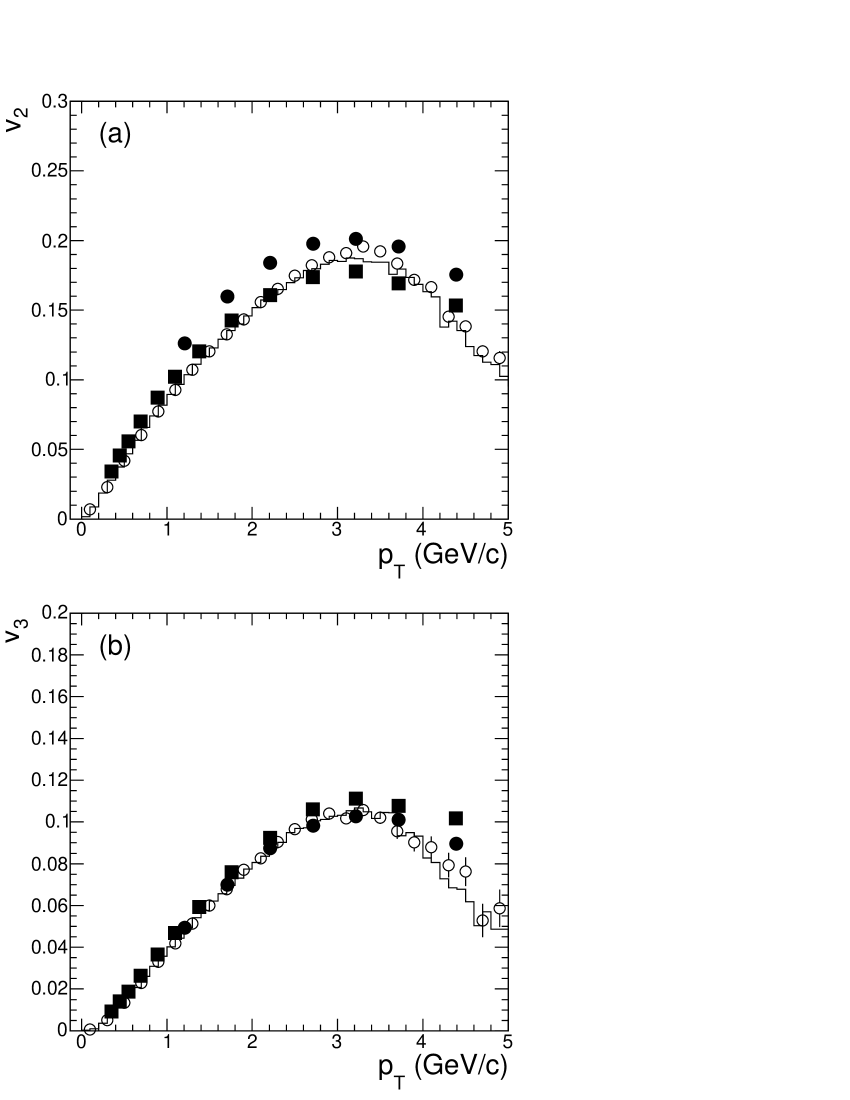
Figure 1: (a) Elliptic flow vs. $p_{\rm T}$ of charged hadrons at $|\eta|<0.8$ in Pb+Pb collisions at $\sqrt{s}=2.76$ TeV with centrality 20$-$25%. Solid circles and solid squares are $v_{2}\{2\}$ and $v_{2}\{LYZ\}$ from CMS Chatrchyan:2012ta , open circles and histogram are $v_{2}\{EP\}$ and $v_{2}(\Psi_{EP,2})$ for HYDJET++ events, respectively. (b) The same as (a) but for the triangular flow $v_{3}(p_{\rm T})$.

Figure 2 shows the correlation radii $R_{out}$, $R_{side}$, and $R_{long}$ of charged pion pairs as functions of the pair transverse momentum $k_{\rm T}$ with $|\eta|<0.8$ in 5% of most central lead-lead collisions at $\sqrt{s}_{\rm NN}=2.76$ TeV. The results of the HYDJET++ simulation are plotted onto the ALICE data Aamodt:2011mr . One can see that the model reproduces the measured $k_{\rm T}$-dependencies of the correlation radii $R_{out}$ and $R_{long}$ very well, and overestimates by about 8% the corresponding distribution for $R_{long}$.

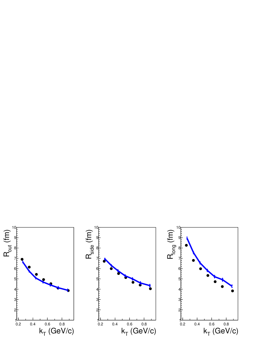
Figure 2: $\pi^{\pm}\pi^{\pm}$ correlation radii as functions of pion pair transverse momentum $k_{\rm T}$ in 5% of most central PbPb collisions at $\sqrt{s}_{\rm NN}=2.76$ TeV. Solid curves show the HYDJET++ calculations, full circles denote the ALICE data Aamodt:2011mr .

To describe both flow harmonics and femtoscopy observables simultaneously the whole set of parameters responsible for geometric and dynamical anisotropy was applied. Now, for the sake of clarity, we start with investigation of individual influence of geometric and dynamical deformations on elliptic flow and related to it second-order femtoscopy radii oscillations. Recall briefly the observed main tendencies in the elliptic flow development and femtoscopy radii distributions with respect to the event plane $\Psi_{EP,2}$ Logg_npa14 . Differential elliptic flow of charged particles, $v_{2}^{ch}(p_{\rm T})$ is positive, $R^{2}_{side}$ has a dip at $\Delta\phi_{2}=\phi_{pair}-\Psi_{EP,2}\simeq\pi/2$, whereas $R^{2}_{out}$ demonstrates quite distinct maximum there. In contrast, distribution $R^{2}_{long}(\Delta\phi_{2})$ appears to be rather flat.

The triangular flow is excluded in HYDJET++ by setting both triangularity parameters, $\varepsilon_{3}$ and $\rho_{3}$, to zero. Then, we consider isotropic expansion model in which the direction of the flow vector of a fluid cell coincides with its velocity vector. In this particular case $\delta_{2}=0$ and the only parameter causing the elliptic anisotropy of particle spectra is $\varepsilon_{2}$. Figure 3 displays the azimuth distributions of the three radii squared together with differential elliptic flow $v_{2}(p_{\rm T})$ for calculations with $\varepsilon_{2}=0.3$ and $\varepsilon_{2}=-0.3$ of Pb+Pb collisions at centrality $20\%\leq\sigma/\sigma_{geo}\leq 30\%$.

We see that for $\varepsilon_{2}=0.3$ the radii squared reproduce qualitatively the trends observed experimentally, whereas the differential elliptic flow is negative at $p_{\rm T}\leq 5$ GeV/$c$. The latter result is obviously wrong. On the other hand, one can get positive $v_{2}(p_{\rm T})$ distribution by switching to negative value $\varepsilon_{2}=-0.3$, but in this case the azimuthal oscillations of $R^{2}_{side}$ and $R^{2}_{out}$ are out-of-phase, as depicted in Fig. 3. Decays of resonances increase all three radii but do not shift the phases of radii oscillations. Therefore, bare geometric anisotropy of the fireball cannot describe the true behavior of both elliptic flow and femtoscopic radii simultaneously.

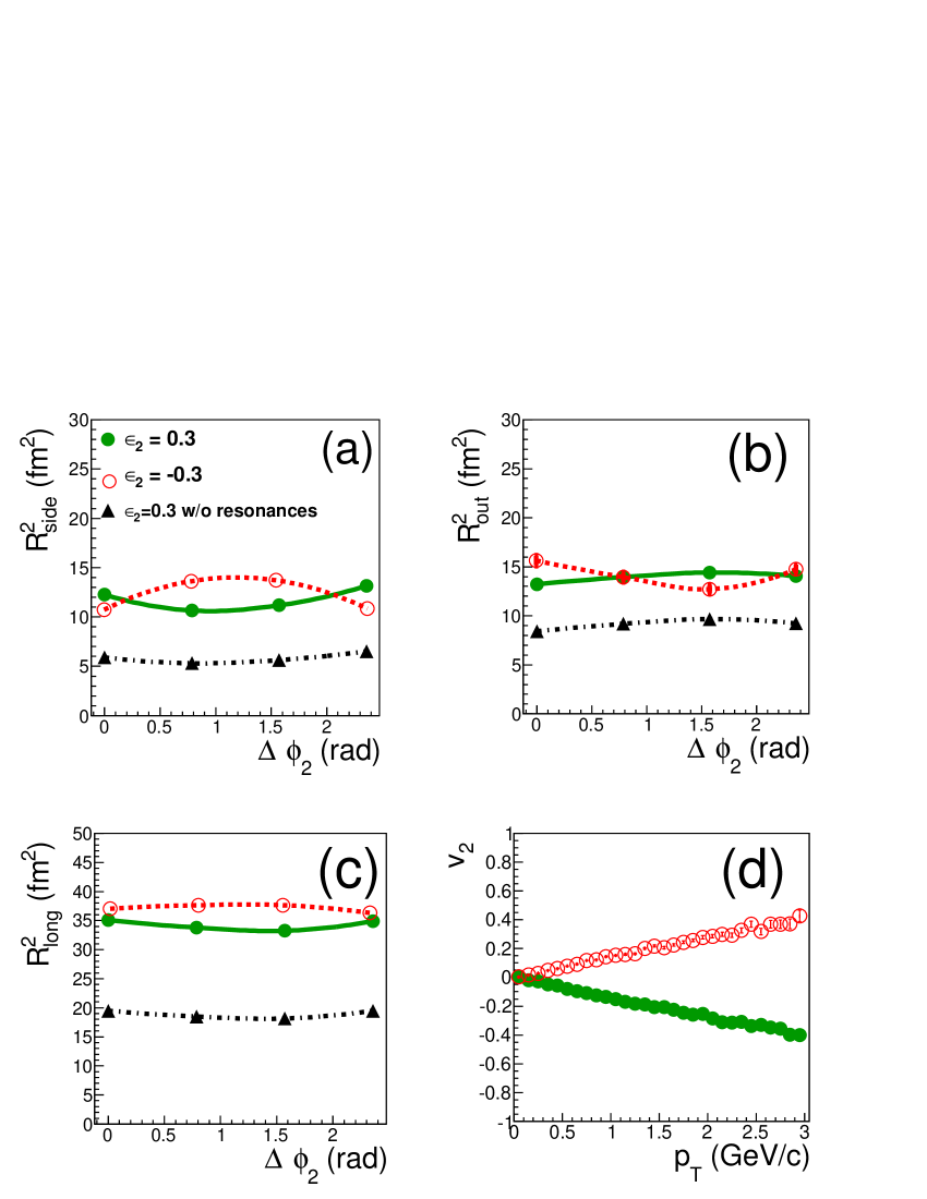
Figure 3: The azimuthal dependence of (a) $R^{2}_{side}$, (b) $R^{2}_{out}$, (c) $R^{2}_{long}$ as a function of $\Delta\phi_{2}=\phi_{pair}-\Psi_{EP,2}$ for the centrality 20–30% and $k_{\rm T}$ range 0.2–2.0 GeV/$c$, and (d) the azimuthal asymmetry coefficient $v_{2}$ versus $p_{\rm T}$. Calculations were performed with the HYDJET++ model using the sets of parameters $\varepsilon_{2}$=0.3, $\delta_{2}$=0, $\varepsilon_{3}$=0, $\rho_{3}$=0 for directly produced particles (solid triangles) and for all particles after the resonance decays (solid circles); and $\varepsilon_{2}=-0.3$, $\delta_{2}$=0, $\varepsilon_{3}$=0, $\rho_{3}$=0 for all particles (open circles). Lines are drawn to guide the eye.

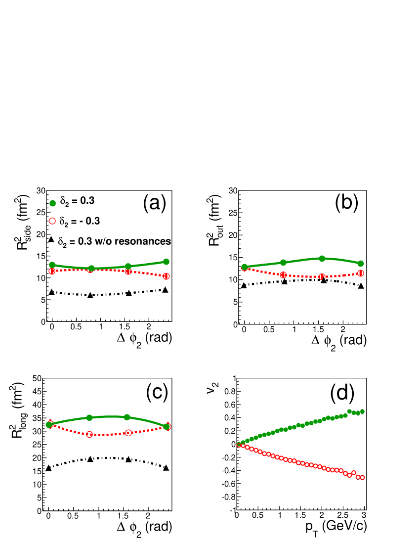
Figure 4: The same as Fig. 3 but with $\varepsilon_{2}=0$, $\delta_{2}=0.3$ for particle spectra before (solid triangles) and after (solid circles) the resonance decays; and $\varepsilon_{2}=0$, $\delta_{2}=-0.3$ for all particles (open circles).

If, in contrast, we will allow for only dynamical elliptic anisotropy in the system by setting $\varepsilon_{2}=0$ and $\delta_{2}=\pm 0.3$, the picture will be drastically changed, as presented in Fig. 4. Positive value of $\delta_{2}$ provides positive $p_{\rm T}$-differential elliptic flow, as well as local minimum of $R_{side}^{2}$ accompanied by local maximum of $R_{out}^{2}$ at $\Delta\phi_{2}\approx\pi/2$, respectively. Similar to the case with pure spatial anisotropy, the positions of extrema in radii oscillations are insensitive to the decays of resonances, although the magnitudes of the oscillations are increased. Calculations with negative value of $\delta_{2}$ result in a completely wrong behavior, namely, in negative elliptic flow and $\pi/2$-shift of the oscillation phase for the femtoscopy radii.

Oscillations of the femtoscopic radii squared $R_{out}^{2},R_{side}^{2}$, and $R_{long}^{2}$ of charged pion pairs with respect to the triangular flow plane $\Psi_{EP,3}$ in Pb+Pb collisions at $\sqrt{s}=2.76$ TeV were studied by ALICE Collaboration in alice_osc_psi3 . Several centralities from 10$-$20% to 40$-$50% were examined, and the general tendencies appeared to be as follows. In the interval $0\leq\Delta\phi_{3}\leq 2,\ \Delta\phi_{3}=\phi_{pair}-\Psi_{EP,3}$, both, $R_{side}^{2}$ and $R_{out}^{2}$, have maxima at $\pi/3$, whereas the distribution $R_{long}^{2}(\Delta\phi_{3})$ is more flat, although the possible oscillations are not ruled out. It is interesting to note, that the signs and positions of the extrema in $R_{\mu}^{2}(\Delta\phi_{2}),\ \mu={out,side}$, distributions in Pb+Pb at LHC energy exactly match those in Au+Au collisions at RHIC ($\sqrt{s}=200$ GeV) phenix_npa13 . The oscillations of $R_{\mu}^{2}$ in the triangular flow plane are more curious. Here $R_{out}^{2}$ reaches maximum at $\Delta\phi_{3}=\pi/3$ in heavy-ion collisions at both RHIC and LHC energy. Distribution $R_{side}^{2}(\Delta\phi_{3})$, however, demonstrates maximum at $\Delta\phi_{3}=\pi/3$ at LHC energy alice_osc_psi3 , and minimum at RHIC energy phenix_npa13 .

Let us investigate the oscillations of femtoscopic radii in geometry dominated scenario, where only the third harmonic of anisotropic flow is present. This means that we set to zero $\varepsilon_{2},\ \delta_{2}$, and $\rho_{3}$, and employ $\varepsilon_{3}\neq 0$ as the only parameter responsible for the triangular flow generation. Two opposite cases, $\varepsilon_{3}=-0.3$ and $\varepsilon_{3}=0.3$, are presented in Fig. 5. For negative value of the spatial triangularity, $R_{side}^{2}$ has a distinct minimum at $\Delta\phi_{3}\simeq 0.75~{}rad$ and smeared maximum at $\Delta\phi_{3}\simeq 1.75~{}rad$, $R_{out}^{2}$ has a maximum at $\Delta\phi_{3}\simeq 1.3~{}rad$, $R_{long}^{2}$ is almost independent on $\Delta\phi_{3}$, and the positive differential triangular flow $v_{3}(p_{\rm T})$ increases with rising transverse momentum. For positive spatial triangularity, the behaviour of $R_{\mu}^{2}$ and $v_{3}(p_{\rm T})$ is completely opposite: $R_{side}^{2}$ has maximum at $\Delta\phi_{3}\approx 0.75~{}rad$ and minimum at $\Delta\phi_{3}\approx 1.75~{}rad$, $R_{out}^{2}$ reaches minimum at $\Delta\phi_{3}\approx 1.3~{}rad$, the distribution $R_{long}^{2}(\Delta\phi_{3})$ is flat within the error bars. Negative for all transverse momenta $v_{3}(p_{\rm T})$ drops with increasing $p_{\rm T}$. Again, decays of resonances increase the femtoscopic radii and magnitudes of their oscillations. However, the positions of extrema of the $R^{2}_{\mu}(\Delta\phi_{3}),\ \mu=out,side,long$ spectra of directly produced hadrons stay put. Therefore, neither of two scenarios, (i) with positive or (ii) with negative $\varepsilon_{3}$, is fully consistent qualitatively with the experimentally observed signals.

In the scenario with dynamical triangular anisotropy domination, one sets $\varepsilon_{2}=\varepsilon_{3}=\delta_{2}=0$, and $\rho_{3}\neq 0$. Again, $\rho_{3}$ can be positive, e.g. $\rho_{3}=0.3$, and negative, $\rho_{3}=-0.3$. Calculations with both sets of parameters are shown in Fig. 6. For positive value of $\rho_{3}$ the experimentally observed behaviour of femtoscopic radii and triangular flow is quantitatively reproduced. Namely, both $R^{2}_{out}$ and $R^{2}_{side}$ have not very distinct maxima at $\Delta\phi_{3}\simeq\pi/3$, and differential triangular flow $v_{3}(p_{\rm T})$ is positive. $R^{2}_{long}$ oscillates slightly, but linear fit within the error bars is still possible. The phases of the oscillations are not shifted after the decays of resonances.

For the case with negative value of the $\rho_{3}$ all three femtoscopic radii squared, $R_{\mu}^{2}(\Delta\phi_{3}),\ \mu=out,side,long$, demonstrate the out-of-phase behaviour, compared to the case with positive $\rho_{3}$, see Fig. 6. Differential triangular flow is also negative. The dynamical anisotropy alone, however, cannot reproduce the magnitudes of the oscillations. Therefore, the final signal appears as a superposition of dynamical anisotropy and geometrical anisotropy.

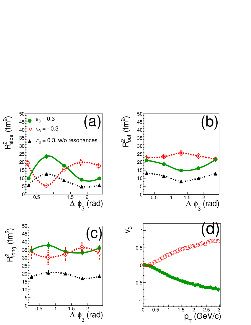
Figure 5: The azimuthal dependence of (a) $R^{2}_{side}$, (b) $R^{2}_{out}$, (c) $R^{2}_{long}$ as a function of $\Delta\phi_{3}=\phi_{pair}-\Psi_{EP,3}$ for the centrality 20–30% and $k_{\rm T}$ range 0.2–2.0 GeV/$c$, and (d) the azimuthal asymmetry coefficient $v_{3}$ versus $p_{\rm T}$. Calculations were performed with the HYDJET++ model using the sets of parameters $\varepsilon_{2}$=0, $\delta_{2}$=0, $\varepsilon_{3}$=0.3, $\rho_{3}$=0 for directly produced particles (solid triangles) and for all particles after the resonance decays (solid circles); and $\varepsilon_{2}$=0, $\delta_{2}$=0, $\varepsilon_{3}=-0.3$, $\rho_{3}$=0 for all particles (open circles). Lines are drawn to guide the eye.

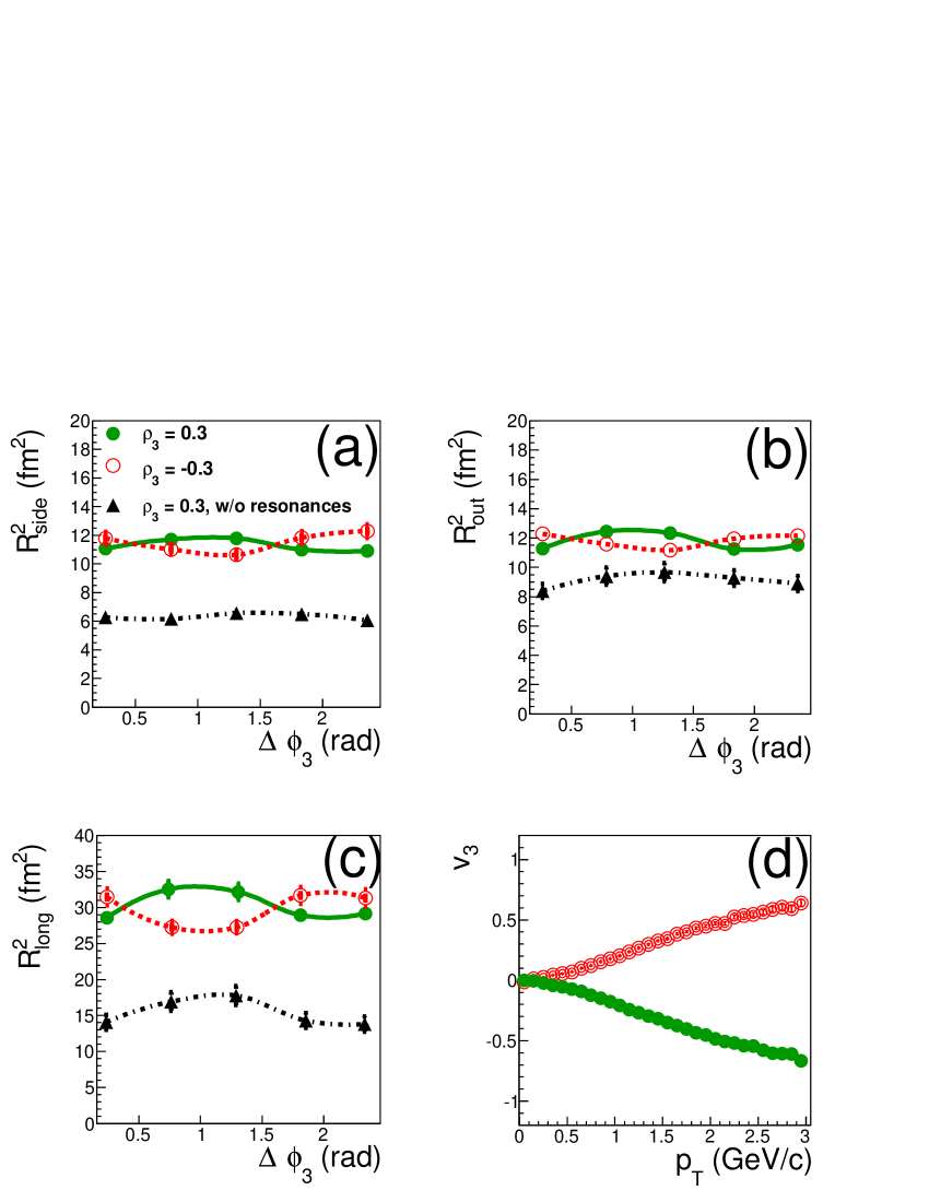
Figure 6: The same as Fig. 5 but with $\varepsilon_{3}=0$, $\rho_{3}=0.3$ for particle spectra before (solid triangles) and after (solid circles) the resonance decays; and $\varepsilon_{3}=0$, $\rho_{3}=-0.3$ for all particles (open circles).

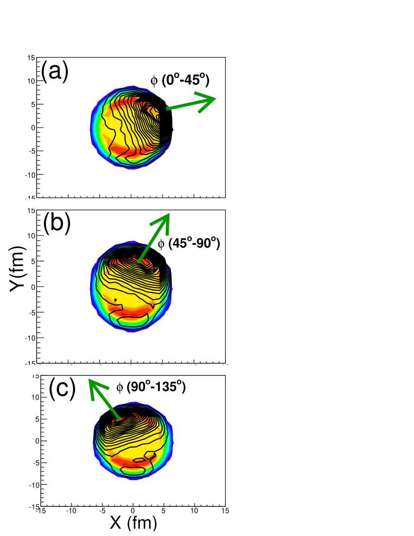
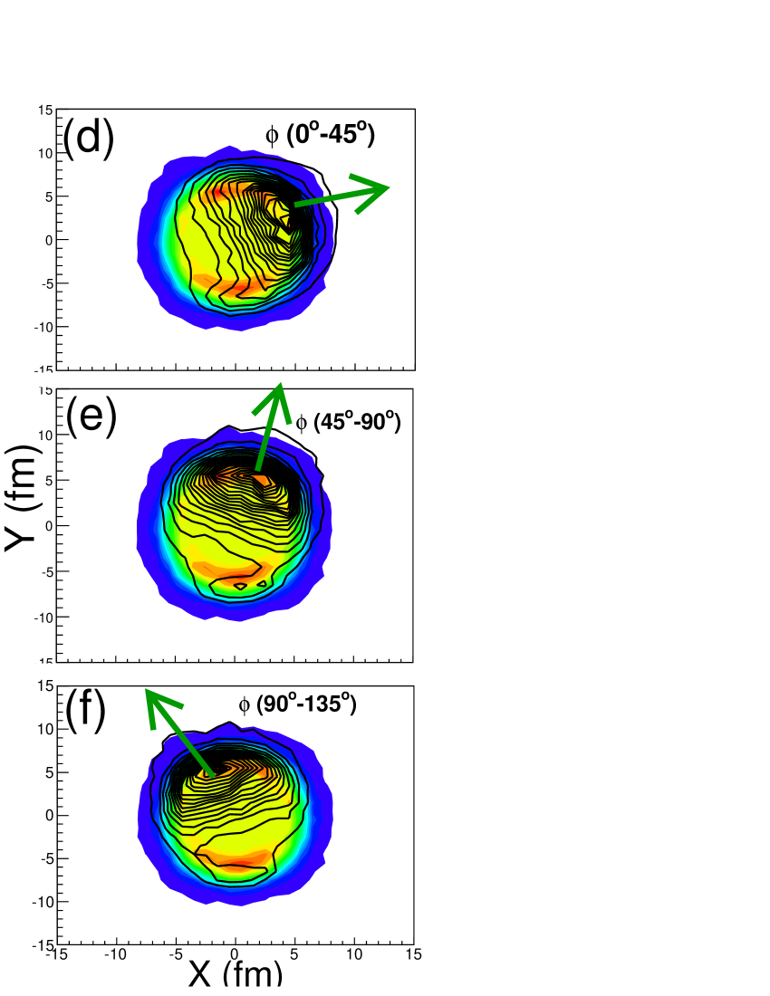
Figure 7: (Color online) Pion emission function before (left column) and after (right column) decays of resonances in the transverse plane of HYDJET++ simulated Pb+Pb collisions at $\sqrt{s}=2.76$ TeV with centrality 20–30%. Only spatial elliptic anisotropy with $\varepsilon_{2}=0.5$ is considered, while the remaining anisotropy parameters $\delta_{2},\varepsilon_{3},$ and $\rho_{3}$ are taken to be zero. Shaded contours are identical for each column and indicate the density of emitted pions. Contour lines show the densities of pions emitted at angles $0<\phi\leq\pi/4$ (upper row), $\pi/4<\phi\leq\pi/2$ (middle row), and $\pi/2<\phi\leq 3\pi/4$ (bottom row), respectively.

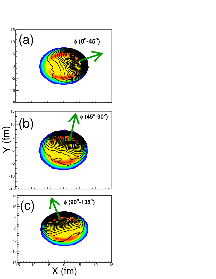
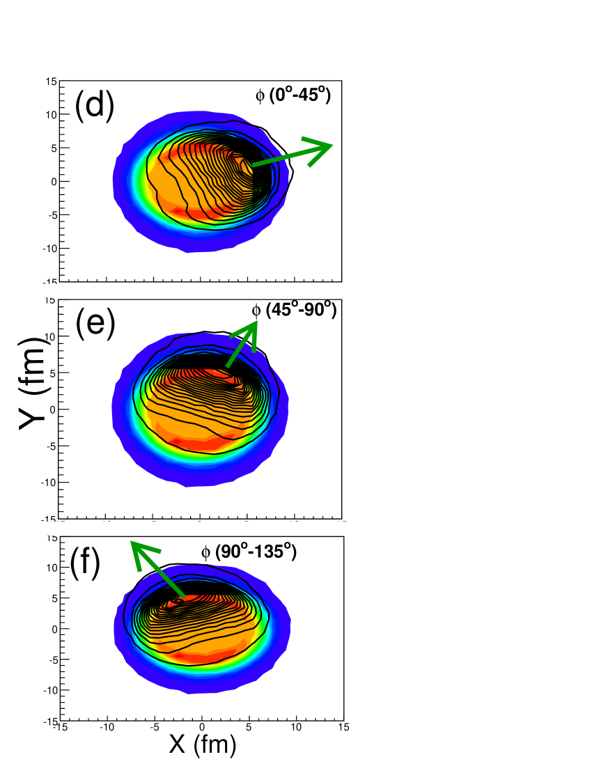
Figure 8: (Color online) The same as Fig. 7 but for calculations with non-zero dynamical elliptic anisotropy, $\delta_{2}=-0.3$, while other anisotropy parameters are equal to zero, $\{\varepsilon_{2},\varepsilon_{3},\rho_{3}\}=0$.

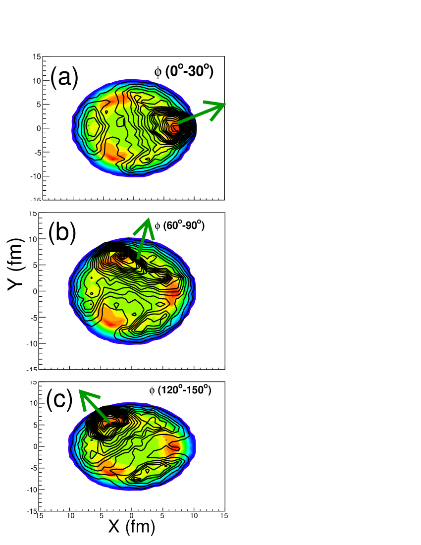
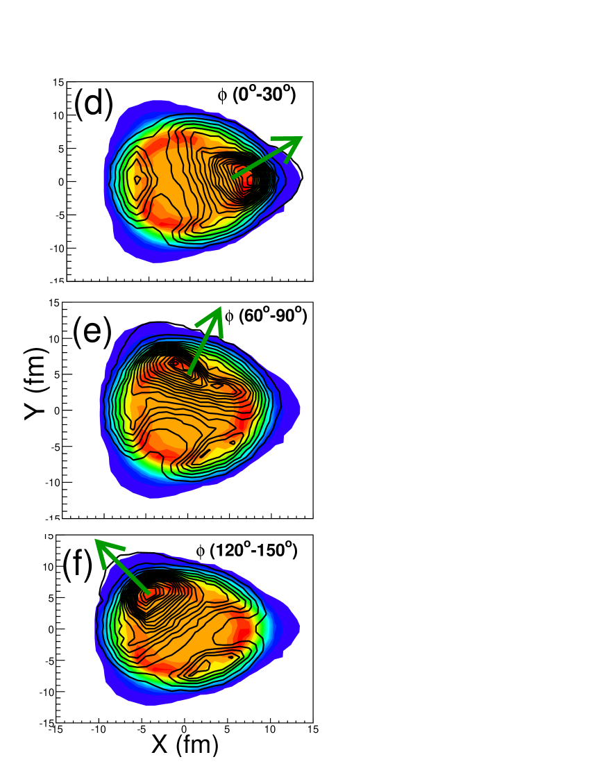
Figure 9: (Color online) The same as Fig. 7 but for calculations with non-zero geometric triangular anisotropy, $\varepsilon_{3}=0.3$, while other anisotropy parameters are equal to zero, $\{\varepsilon_{2},\delta_{2},\rho_{3}\}=0$. Contour lines show the densities of pions emitted at angles $0<\phi\leq\pi/6$ (upper row), $\pi/3<\phi\leq\pi/2$ (middle row), and $2\pi/3<\phi\leq 5\pi/6$ (bottom row), respectively.

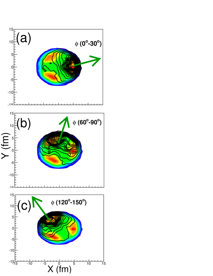
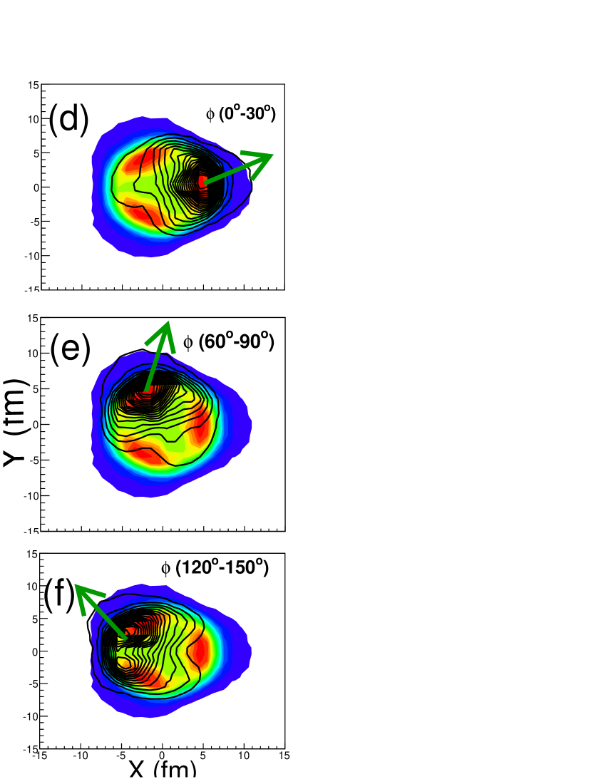
Figure 10: (Color online) The same as Fig. 7 but for calculations with non-zero dynamical triangular anisotropy, $\rho_{3}=0.5$, while other anisotropy parameters are taken to be zero, $\{\varepsilon_{2},\delta_{2},\varepsilon_{3}\}=0$.

The femtoscopy analysis allows us to probe the emission zones, also known as “‘homogeneity lengths”, rather than the sizes of the whole source led04 . To study the size and shape of the particle sources in HYDJET++, we plot in Figs. 7$\div$10 the transverse plane emission densities of pions, radiated directly from the freeze-out hypersurface (left columns), and of all pions, produced both at the freeze-out hypersurface and from the resonance decays (right columns). Figure 7 corresponds to the presence of only geometric ellipticity, $\varepsilon_{2}=0.5$, while other dynamic and spatial sources of the system ellipticity and triangularity are absent, i.e. $\delta_{2}=\varepsilon_{3}=\rho_{3}=0$. Other figures illustrate the cases with $\delta_{2}=-0.3$ and $\varepsilon_{2}=\varepsilon_{3}=\rho_{3}=0$ (Fig. 8), with $\varepsilon_{3}=0.3$ and $\varepsilon_{2}=\delta_{2}=\rho_{3}=0$ (Fig. 9), and with $\rho_{3}=0.5$ and $\varepsilon_{2}=\delta_{2}=\varepsilon_{3}=0$ (Fig. 10), respectively. Three angular areas of the pion emission are considered for each of the anisotropies. For the bare elliptic anisotropy we opted for (i) $0<\phi\leq\pi/4$, (ii) $\pi/4<\phi\leq\pi/2$, and (iii) $\pi/2<\phi\leq 3\pi/4$, shown in Fig. 7 and Fig. 8, whereas for the triangular anisotropy the choice is (i) $0<\phi\leq\pi/6$, (ii) $\pi/3<\phi\leq\pi/2$, and (iii) $2\pi/3<\phi\leq 5\pi/6$, displayed in Fig. 9 and Fig. 10. Let us compare first emission functions corresponding to geometric and dynamical elliptic anisotropies, presented in Fig. 7 and Fig. 8. One can see that the same-density contours of pion emission are much smoother for dynamical anisotropy compared to the spatial one. Also, the spatial anisotropy provides stronger difference between the emitting zones at three different angles in contrast to the dynamical anisotropy. This circumstance explains the stronger angular dependence of $R^{2}_{out}(\Delta\phi_{2})$ and $R^{2}_{side}(\Delta\phi_{2})$ for geometric anisotropy seen in Fig. 3. Similar difference between the spatial and dynamical anisotropy was also found recently in the Buda-Lund model in CTCL_17 . Pions coming from the decays of resonances enlarge the emission areas and make the density contours smoother, as seen in right windows of both Fig. 7 and Fig. 8.

The pion emission functions for the systems with only geometric or only dynamical triangularity, depicted in Fig. 9 and in Fig. 10, respectively, reveal similar tendencies. First of all, the spatial triangularity produces much stronger difference for the emitting areas in three azimuthal directions compared to the dynamical triangularity. Then, as in the elliptic anisotropy case, decays of resonances lead to rounding of the pion density contours. The triangular profile of the outher area of transverse pion emission becomes quite distinct after the resonance decays. All four systems shown in Figs. 7$\div$10 demonstrate a clear angular dependence of the homogeneity regions discussed, e.g., in Wiedemann:1997cr ; H_prl99 in addition to that given by the set of Eqs.(1). It is worth noting also that the non-Gaussian shapes of the homogeneity regions make complicated restoration of the shape and size of the source by the standard femtoscopic analysis.

4 Conclusions

Second- and third-order oscillations of the femtoscopic radii $R_{side}^{2},R_{out}^{2}$, and $R_{long}^{2}$ in Pb+Pb collisions at $\sqrt{s}=2.76$ TeV were studied within the HYDJET++ model together with the differential elliptic and triangular flow. For each type of the flow harmonics the model assumes two parameters. One of them is responsible for spatial, or geometric, deformation of the freeze-out hypersurface, whereas the other parameter is accountable for the dynamical flow anisotropy, respectively. By switching on and off of these key parameters one can investigate the influence of separated spatial and dynamical anisotropy effects on the flow harmonics and on the femtoscopic radii. Our study indicates that merely geometric anisotropy cannot reproduce simultaneously the correct phase of the second- and third-order oscillations of the femtoscopic radii and the corresponding differential flow harmonics. Dynamical flow anisotropy, in contrast, provides correct qualitative description of both $p_{\rm T}$-dependence of the flow harmonics and the phases of the femtoscopic radii oscillations.

The spatial anisotropy, however, reveals stronger difference between the emitting zones of pions, radiated at different angles. This leads to stronger azimuthal oscillations of femtoscopic radii in case with spatial ellipticity or triangularity compared to the case with the dynamical ones. Our findings are in line with the results of other models PSH_13 ; CTCL_17 . Decays of resonances provide significant increase of the emitting areas in the both planes of elliptic and triangular flow. Also, the resonance decays make the radii oscillations more pronounced, but they do not change the phases of the oscillations. For the quantitative description of the flow and the femtoscopy observables one has to use the full set of geometric and dynamical anisotropy parameters.