Standard Model Theory

Abstract:

The field of precision calculations for Standard Model processes at the LHC has experienced enormous progress in recent years. This talk highlights some examples from the physics of parton distribution functions, jets, electroweak gauge bosons and Higgs bosons.

1 Introduction

The CERN Large Hadron Collider (LHC) was built to explore the validity of the Standard Model (SM) of particle physics at energy scales ranging from the electroweak (EW) scale $\sim 100\,\mathrm{GeV}$ up to energies of some TeV and to search for new phenomena and new particles in this energy domain. The discovery of a Higgs particle at LHC Run 1 in 2012 was a first big achievement in this enterprise. Since first studies of the properties of this Higgs particle (spin, CP parity, couplings to the heaviest SM particles) show good agreement between measurements and SM predictions, the SM is in better shape than ever to describe all known particle phenomena up to very few exceptions (Dark Matter, some tension in the measured anomalous magnetic moment of the muon, etc.). In view of the absence of spectacular new-physics signals in LHC data, this means that any deviation from the SM hides in small and subtle effects. To extract those differences from data, both experimental analyses and theoretical predictions have to be performed with the highest possible accuracy, i.e. precision can be the key to new discoveries. Precise theoretical predictions have to include quantum corrections, both of the strong and EW interaction.

This short review summarizes some recent highlights of precision calculations for the LHC—a field that has seen enormous progress in the recent years. The calculation of perturbative next-to-leading-order (NLO) QCD and EW corrections has been successfully automated up to particle multiplicities of roughly 4–6 (depending on the complexity of the process) upon combining multi-purpose Monte Carlo generators or integrators with automated one-loop matrix-element generators. At the next-to-next-to-leading-order (NNLO) level QCD calculations have been completed for the most important $2\to 2$ particle scattering processes at the LHC, and even next-to-next-to-next-to-leading order (NNNLO) corrections have been made possible for two Higgs-boson production channels using specific approximations. This progress in fixed-order calculations goes in parallel with new achievements in the all-order calculation of leading corrections, such as analytic QCD resummations at higher and higher levels of accuracy and numerically working parton showers. For example, the matching of fixed-order calculations to QCD parton showers is meanwhile standard at NLO, and first results exist at the NNLO level [1]; the inclusion of photon-emission in the NLO matching has been performed for some processes as well [2] (see also Ref. [3]). Parton showers describe jet emission beyond fixed order in some logarithmic approximation. For cases in which full NLO precision is desirable in higher jet multiplicities, merging techniques are available to combine NLO calculations for a specific event topology together with $n=0,1,2,...$ jets, while avoiding double-counting of jet activity.

In the following we discuss some recent advances in different directions, including the issue of the photon density in the proton, QCD corrections to jet physics, EW corrections to weak gauge-boson production processes, and the global status of Higgs production cross sections. Highlights from top-quark [4] and flavour physics [5] as well as more details and examples for progress in higher-order calculations [6, 7] can be found elsewhere in these proceedings.

2 The photon density of the proton

Collinear photon emission off (anti)quark partons of the proton leads to logarithmic mass singularities in the calculation of NLO EW corrections to partonic cross sections, just as gluon emission in NLO QCD calculations. Analogous to the absorption of those QCD initial-state singularities into the parton distribution functions (PDFs) of the proton, the corresponding photonic singularities are absorbed into the PDFs as well. This PDF redefinition naturally leads to a photon PDF, whose dependence on its factorization scale $\mu$ is ruled by the DGLAP evolution equations, which include the photon PDF just like the other quark, antiquark, and gluon PDFs.

Among the usually employed PDF sets, MRST2004qed [12] was the first that provided a photon PDF, which, however, was completely model driven and did not include an error estimate in its original version (a later version provides the error band shown in Fig. 1 below). About ten years later, the NNPDF group provided photon PDFs in the NNPDF23qed [13] and NNPDF30qed [14] PDF sets, which were derived from experimental data (deep-inelastic ${\mathrm{e}}{\mathrm{p}}$ scattering, Drell–Yan-like W/Z production) and, thus, suffered from large errors, which could be as large as $100\%$. Upon combining constraints from data with model assumptions, the photon PDF in the CT14qed set [15] was accurate at the level of $10{-}20\%$. The situation was drastically improved in 2016 with the advent of the LUXqed photon PDF [16], which was derived by exploiting the trick that hadronic collisions mediated by virtual photons only can be equivalently described by using a photon PDF or by the parametrization of the hadronic tensor by the structure functions $F_{2}$ and $F_{\mathrm{L}}$. In this way, it is possible to derive a relation between the photon PDF $f_{\gamma}(x,\mu^{2})$ and the structure functions,

$${xf_{\gamma}(x,\mu^{2})} = \frac{1}{2\pi\alpha(\mu^{2})}\int_{x}^{1}\frac{\mathrm{d}z}{z}\,\biggl{\{}\,\int^{\mu^{2}/(1-z)}_{x^{2}m_{\mathrm{p}}^{2}/(1-z)}\frac{\mathrm{d}Q^{2}}{Q^{2}}\,\alpha(Q^{2})^{2}\,\biggl{[}\biggl{(}zp_{\gamma q}(z)+\frac{2x^{2}m_{\mathrm{p}}^{2}}{Q^{2}}\biggr{)}\,{F_{2}\Big{(}\frac{x}{z},Q^{2}\Big{)}}$$ (1)

$$\hskip 120.00018pt{}-z^{2}\,{F_{\mathrm{L}}\Big{(}\frac{x}{z},Q^{2}\Bigr{)}}\biggr{]}-\alpha(\mu^{2})^{2}\,z^{2}\,{F_{2}\Big{(}\frac{x}{z},\mu^{2}\Big{)}}\biggr{\}},\hskip 20.00003pt$$

which can be numerically evaluated from data on $F_{2}(x,Q^{2})$ and $F_{\mathrm{L}}(x,Q^{2})$. In Eq. (1), $m_{\mathrm{p}}$ is the proton mass and $p_{\gamma q}(z)$ the $q\to\gamma q$ splitting function.

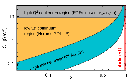
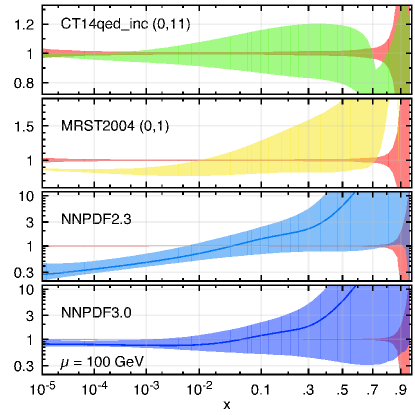
Figure 1: Left: breakup of the $(x,Q^{2})$ plane in terms of the $F_{2}(x,Q^{2})$ and $F_{\mathrm{L}}(x,Q^{2})$ data used in Eq. (1). Right: ratio of photon PDFs from some common PDF sets (with uncertainty bands) to the LUXqed photon PDF (uncertainty band in red). (Taken from Ref. [16].)

The l.h.s. of Fig. 1 illustrates the coverage of the $(x,Q^{2})$ plane by data from different experiments. Note that the region at $x=1$ contains the contribution from elastic scattering, where the proton does not break up in the collision. The r.h.s., finally, shows the comparison of the mentioned determinations of the photon PDF, normalized to LUXqed, with respective error bands. The LUXqed photon PDF is good within $1{-}2\%$ in the typical $x$ range of LHC physics and, thus, even the best known of all PDFs.

Partonic channels with initial-state photons exist for every scattering reaction at the LHC, but their contribution typically is part of the EW corrections and at the level of few percent. Exceptions are processes where $\gamma\gamma$, ${\mathrm{g}}\gamma$, or $q\gamma$ collisions already appear in lowest order, or processes with W bosons in the final state. The enhancement in the latter is due to the fact that initial-state photons can couple to $t$-channel W bosons, leading to enhanced forward W production—a mechanism that is not overwhelmed by quark–gluon scattering. In the extreme case of triple-W production [17, 18], the contribution from $q\gamma$ scattering is about $12\%$ (relative to the leading-order prediction) at the LHC running with a centre-of-mass (CM) energy of $13\,\mathrm{TeV}$.

3 Jet production

Investigating jet production at the LHC is not only important as consistency check on the validity and our understanding of QCD, it provides also important information on PDFs and another possibility to measure the strong coupling constant $\alpha_{\mathrm{s}}$.

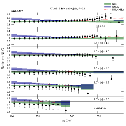
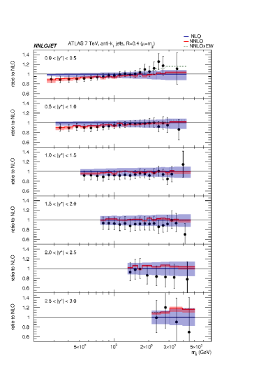
Figure 2: Single-jet inclusive (left) and di-jet (right) differential cross sections at NNLO and NLO QCD normalized to NLO QCD in comparison to ATLAS data, with corresponding scale uncertainty bands. The inclusion of EW corrections is indicated by the dashed lines. (Taken from Refs. [20, 21].)

Last but not least, jet production is an ubiquitous background to other processes. On the theory side, it is crucial to control QCD corrections to jet production to the highest possible level, a task that is complicated for various reasons: Corrections are large due to high powers of $\alpha_{\mathrm{s}}$, jet multiplicities can be high, a perturbatively stable definition of jets requires great care, etc..

Recently, great progress was made in predicting cross sections for single-jet inclusive [20] and di-jet [21] production at the NNLO QCD level in leading-colour approximation. Figure 2 shows some results on the transverse-momentum ($p_{\mathrm{T}}$) spectrum of the leading jet in single-jet inclusive production as well as the di-jet invariant mass ($m_{\mathrm{jj}}$) distribution in di-jet production, categorized according to rapidity regions. In the transition from NLO to NNLO QCD predictions, the scale uncertainty, which is indicated by the corresponding bands, is reduced from typically $10{-}20\%$ to some percent at large transverse momenta or large invariant masses. The NNLO corrections are quite sizeable, and the slight tensions between NNLO prediction and data most likely are due to the neglect or the approximative inclusion of the NNLO contributions in the determination of the employed PDF sets, so that a significant impact of the new NNLO results on PDF fits can be expected. It is also interesting to note that data start to be sensitive to EW corrections [22] as well, whose impact is indicated by dashed lines in the plots.

4 Electroweak gauge-boson production

Pair production of massive EW gauge bosons is interesting at the LHC both as signal and background process. As signal, it bears direct information on the non-Abelian triple-gauge-boson interactions, which are sensitive to physics beyond the SM. As background, it is relevant to many searches for new physics and, most notably, to analyses of Higgs bosons based on the four-body decays ${\mathrm{H}}\to{\mathrm{W}}{\mathrm{W}}/{\mathrm{Z}}{\mathrm{Z}}\to 4\,$leptons. Note, however, that in the latter case at least one of the two W or Z bosons is far off its mass shell, so that predictions based on on-shell W- or Z-boson pairs cannot be used.

.8

Figure 3: Sample diagrams for four-fermion production in $\bar{q}q$ annihilation. Left: structural diagram for the factorizable contributions of a DPA; middle: LO diagram without two intermediate W bosons; right: hexagon loop diagram.

In previous years, the theoretical descriptions of these processes made major leaps: QCD predictions were pushed to NNLO [23] (+ $gg$ channels to NLO [24]), and EW NLO corrections, which were only known for on-shell W/Z bosons [25] or in the form of resonance expansions [26] before, were generalized to full off-shell calculations for four-lepton production [27, 28, 29, 30] using the complex-mass scheme [31] for a gauge-invariant treatment of the resonances. Figure 3 illustrates on its l.h.s. the structure of loop diagrams of the so-called factorizable corrections which furnish the dominating contributions in an expansion of amplitudes about the resonance poles. The leading term of such an expansion is known as double-pole approximation (DPA). The middle and left diagrams in Fig. 3 show tree-level and one-loop diagrams that would be neglected in a leading-order (LO) or NLO DPA, respectively. The l.h.s. of Fig. 4 shows the NLO QCD and EW corrections to the transverse-momentum spectrum of a charged lepton in the process ${\mathrm{p}}{\mathrm{p}}\to{\mathrm{e^{+}}}{\mathrm{e^{-}}}\nu\bar{\nu}$ [29], which is dominated by W-pair production.

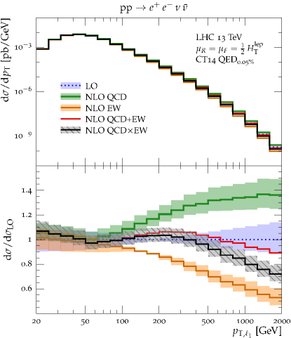
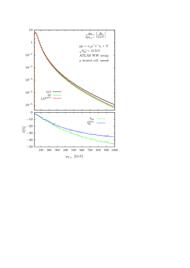
Figure 4: Transverse-momentum distributions of charged leptons in $pp\to e^{+}e^{-}\nu\bar{\nu}$ (left) and in $pp\to\nu_{\mu}\mu^{+}e^{-}\bar{\nu}_{e}$ (right), with relative corrections shown in the lower panels, as described in the text. On the r.h.s. NLO EW corrections to the $\bar{q}q$ channels obtained from a full four-fermion calculation are compared to results from a DPA. (Taken from Refs. [28, 29].)

The EW corrections show the known Sudakov enhancement to several $10\%$ in the TeV range, a regime explored by the LHC deeper and deeper in the next years. The r.h.s. of the figure compares results of the full $2\to 4$ off-shell calculation [28] of the EW corrections to ${\mathrm{p}}{\mathrm{p}}\to\nu_{\mu}\mu^{+}{\mathrm{e^{-}}}\bar{\nu}_{\mathrm{e}}$ with a corresponding DPA [26]. While the DPA represents a very good approximation whenever two W resonances dominate (integrated cross sections, rapidity distributions, momentum spectra at smaller energies, etc.), it fails for transverse lepton momenta at high

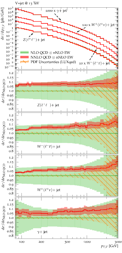
Figure 5: $V+$jet spectra predicted at (N)NLO QCD $\otimes$ nNLO EW, where the lower panels show the relative impact of (N)NLO QCD $\otimes$ nNLO EW over NLO QCD $\otimes$ nNLO EW, together with the corresponding uncertainty bands (nNLO EW is the sum of NLO EW and leading NNLO EW Sudakov logarithms). PDF uncertainties are included as hashed orange bands. (Taken from Ref. [32].)

energies, where the DPA misses corrections to singly-resonant diagrams as shown in the middle of Fig. 3, which can be viewed as W bremsstrahlung to Drell–Yan-like lepton pair production.

Figure 4 (left) also illustrates the issue of combining QCD and EW corrections by comparing the two extreme variants of simply adding (QCD$+$EW) or factorizing (QCD$\times$EW) QCD and EW corrections. If both types of corrections become large the differences between the two possibilities can get large, but the difference itself is an overly conservative estimate of the uncertainty of the combination, because leading corrections are known to factorize to a large extent. This and other issues in the determination of a realistic estimate of theory and parametric uncertainties in predictions were analyzed in Ref. [32], where EW vector-boson+jet production was considered as background to Dark Matter searches at high transverse vector-boson momenta $p_{\mathrm{T},V}$ at the LHC. Schematically, Monte Carlo (MC) and theory (TH) uncertainties are introduced in Monte Carlo predictions via reweighting,

$$\frac{\mathrm{d}}{\mathrm{d}x}\,\frac{\mathrm{d}}{\mathrm{d}\vec{y}}\,\sigma(\vec{\varepsilon}_{\mathrm{MC}},{\vec{\varepsilon}_{\mathrm{TH}}})$$

$$= \frac{\mathrm{d}}{\mathrm{d}x}\,\frac{\mathrm{d}}{\mathrm{d}\vec{y}}\,\sigma_{\mathrm{MC}}(\vec{\varepsilon}_{\mathrm{MC}})\,\times\,\left(\frac{\frac{\mathrm{d}}{\mathrm{d}x}\,{\sigma_{\mathrm{TH}}}({\vec{\varepsilon}_{\mathrm{TH}}})}{\frac{\mathrm{d}}{\mathrm{d}x}\,\sigma_{\mathrm{MC}}(\vec{\varepsilon}_{\mathrm{MC}})}\right),$$

where fully differential MC cross sections $\sigma_{\mathrm{MC}}$ are reweighted by the ratio to a state-of-the-art TH prediction $\sigma_{\mathrm{TH}}$ which is only differential in one (but distinctive) kinematical variable $x$, which was taken to be $x=p_{\mathrm{T},V}$ ($\vec{y}$ denotes the remaining phase-space variables). The nuisance parameters $\vec{\varepsilon}_{\mathrm{MC/TH}}$ control the impact of scale uncertainties, missing higher-order effects, the combination of QCD and EW corrections, PDF uncertainties, and correlations between different processes (${\mathrm{W}}/{\mathrm{Z}}/\gamma+{}$jet) and phase-space regions. Figure 5 illustrates the resulting uncertainties, revealing surprisingly good precision even for $p_{\mathrm{T},V}$ in the TeV range. Perturbative cross-section uncertainties (combined quadratically) are about $5\%$ and PDF uncertainties (correlated among processes) about $5{-}10\%$, leading to a W/Z cross-section ratio uncertainty (not shown) of about $1{-}2\%$. The detailed results from this study are, of course, specific to ${\mathrm{W}}/{\mathrm{Z}}/\gamma+$jet production, but the methodology can be transferred to other processes.

As a last example from EW vector-boson physics, we consider the scattering of massive EW vector-bosons (see also Ref. [33]), such as ${\mathrm{W}}{\mathrm{W}}\to{\mathrm{W}}{\mathrm{W}}$, which is not only sensitive to triple and quartic gauge-boson self-interactions, but also to the mechanism of EW symmetry breaking via off-shell Higgs boson exchange in spontaneously broken gauge theories (or any other related effect in other theories). These processes are part of $VV+2$jet production processes at the LHC, which has reported first successful analyses for like-sign W-boson pairs. The existence of 4 leptons and 2 jets in the final state renders theoretical predictions with higher-order corrections to such processes extremely demanding.

Figure 6: Sample LO and NLO diagrams for vector-boson scattering at the LHC.

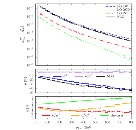
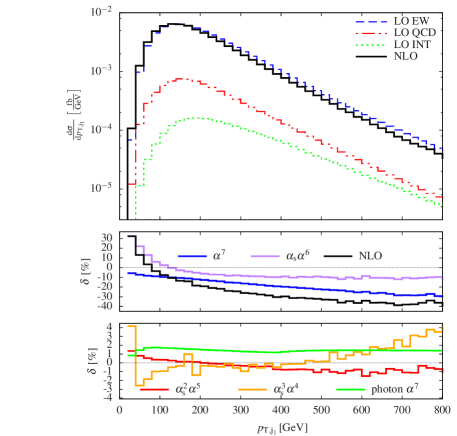
Figure 7: Transverse-momentum distributions of the muon (left) and the leading jet (right) and corresponding relative corrections (lower panels) for the process $pp\to\mu^{+}\nu_{\mu}e^{+}\nu_{e}\mathrm{jj}+X$ at the LHC with CM energy 13 TeV. (Taken from Ref. [35].)

Recently first results from an NLO calculation for the full $2\to 6$ particle process involving like-sign W pairs were presented in Refs. [34, 35], based on the one-loop matrix-element generator Recola [36] and the numerical one-loop integral library Collier [37]. The diagrams in Fig. 6 show that already at LO different perturbative orders $\propto\alpha_{\mathrm{s}}^{m}\alpha^{n}$ contribute to the cross section, leading to four different orders at NLO. The pure QCD corrections to the two LO channels indicated in Fig. 6 were already calculated in Refs. [38]e

In Fig. 7 the impact of those orders is shown separately for the transverse-momentum spectra of a charged lepton and the leading outgoing jet for typical selection cuts for vector-boson scattering. As expected, the contributions $\propto\alpha_{\mathrm{s}}\alpha^{6}$ or $\alpha^{7}$ with the highest powers in the EW couplings deliver the largest corrections, with up to some $10\%$ when the TeV range is approached, rendering those contributions important in future data analyses. On the other hand, photon-induced channels (shown as green lines) contribute to the signal only a few percent.

5 Higgs-boson production

Since many years the LHC Higgs Cross Section Working Group provides state-of-the-art predictions for the various Higgs-boson production and decay channels, as well as details of many other phenomenological aspects and strategies in Higgs physics. As an important example taken from the recent CERN Yellow Report [39], the l.h.s. of Figure 8 shows an overview of the cross sections of various Higgs-boson production channels in the SM as function of the CM energy $\sqrt{s}$ of a pp collider, together with the bands reflecting the combined theoretical and PDF uncertainties. The table on the r.h.s. compiles the orders of magnitude of the uncertainties and the impact of QCD and EW corrections for the most important channels. Impressively, the uncertainties in the QCD-driven channels (ggF, ttH) are below $10\%$ (see also Ref. [40]) and in the EW-driven channels (VBF, WH, ZH) below $5\%$. To reach this high level of accuracy, in most cases QCD corrections beyond NLO and EW corrections at NLO are required. For details, we have to refer to Ref. [39] and references therein. As highlights, we just mention the level of NNNLO in QCD achieved for gluon–gluon fusion (ggF) [41] and vector-boson fusion (VBF) [42] (although the latter is not yet included on the l.h.s. of Fig. 8) in appropriate approximations.

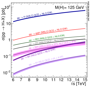
$\sqrt{s}=$ Uncertainties NLO/NNLO/NNNLO $14\,\mathrm{TeV}$ theory PDF4LHC QCD EW ggF $6\%$ $3\%$ ${>}100\%$ $5\%$ VBF $1\%$ $2\%$ $5\%$ $5\%$ WH $1\%$ $2\%$ $20\%$ $7\%$ ZH $4\%$ $2\%$ $35\%$ $5\%$ ttH $9\%$ $4\%$ $20\%$ $1{-}2\%$

Figure 8: Higgs production cross sections at the LHC and corresponding uncertainty bands (left), as given by the LHCHXSWG [39], and estimates of theory and PDF uncertainties as well as the typical size of QCD and EW corrections for the most important channels.

References

-
[1]
S. Alioli et al.,
JHEP 1406 (2014) 089
[arXiv:1311.0286 [hep-ph]] and
Phys. Rev. D 92 (2015) no.9, 094020
[arXiv:1508.01475 [hep-ph]];
S. Höche et al., Phys. Rev. D 91 (2015) no.7, 074015 [arXiv:1405.3607 [hep-ph]] and Phys. Rev. D 90 (2014) no.5, 054011 [arXiv:1407.3773 [hep-ph]]. -
[2]
L. Barze et al.,
Eur. Phys. J. C 73 (2013) no.6, 2474
[arXiv:1302.4606 [hep-ph]];
A. Mück and L. Oymanns, JHEP 1705 (2017) 090 [arXiv:1612.04292 [hep-ph]];
C. M. Carloni Calame et al., arXiv:1612.02841 [hep-ph]. - [3] A. Vicini, these proceedings.
- [4] M. Czakon, these proceedings.
- [5] S. Gori, these proceedings.
- [6] G. Zanderighi, these proceedings.
- [7] A. Huss, these proceedings.
- [8] F. Giuli, these proceedings.
- [9] A. Glazov, these proceedings.
- [10] A. Guffanti, these proceedings.
- [11] G. Sborlini, these proceedings.
- [12] A. D. Martin et al., Eur. Phys. J. C 39 (2005) 155 [hep-ph/0411040].
- [13] R. D. Ball et al. [NNPDF Collaboration], Nucl. Phys. B 877 (2013) 290 [arXiv:1308.0598 [hep-ph]].
- [14] R. D. Ball et al. [NNPDF Collaboration], JHEP 1504 (2015) 040 [arXiv:1410.8849 [hep-ph]].
- [15] C. Schmidt et al., Phys. Rev. D 93 (2016) no.11, 114015 [arXiv:1509.02905 [hep-ph]].
- [16] A. Manohar et al., Phys. Rev. Lett. 117 (2016) no.24, 242002 [arXiv:1607.04266 [hep-ph]] and arXiv:1708.01256 [hep-ph].
- [17] Y. B. Shen et al., Phys. Rev. D 95 (2017) no.7, 073005 [arXiv:1605.00554 [hep-ph]].
- [18] S. Dittmaier et al., JHEP 1709 (2017) 034 [arXiv:1705.03722 [hep-ph]].
- [19] Z. Trocsanyi, these proceedings.
- [20] J. Currie et al., Phys. Rev. Lett. 118 (2017) no.7, 072002 [arXiv:1611.01460 [hep-ph]].
- [21] J. Currie et al., arXiv:1705.10271 [hep-ph].
-
[22]
S. Dittmaier et al.,
JHEP 1211 (2012) 095
[arXiv:1210.0438 [hep-ph]];
J. M. Campbell et al., Phys. Rev. D 94 (2016) no.9, 093009 [arXiv:1608.03356 [hep-ph]];
R. Frederix et al., JHEP 1704 (2017) 076 [arXiv:1612.06548 [hep-ph]]. -
[23]
F. Cascioli et al.,
Phys. Lett. B 735 (2014) 311
[arXiv:1405.2219 [hep-ph]];
T. Gehrmann et al., Phys. Rev. Lett. 113 (2014) 21, 212001 [arXiv:1408.5243 [hep-ph]];
M. Grazzini et al., Phys. Lett. B 750 (2015) 407 [arXiv:1507.06257 [hep-ph]]; JHEP 1608 (2016) 140 [arXiv:1605.02716 [hep-ph]] and JHEP 1705 (2017) 139 [arXiv:1703.09065 [hep-ph]]. - [24] F. Caola et al., Phys. Rev. D 92 (2015) no.9, 094028 [arXiv:1509.06734 [hep-ph]]; Phys. Lett. B 754 (2016) 275 [arXiv:1511.08617 [hep-ph]] and JHEP 1607 (2016) 087 [arXiv:1605.04610 [hep-ph]].
-
[25]
A. Bierweiler et al.,
JHEP 1211 (2012) 093
[arXiv:1208.3147 [hep-ph]].
JHEP 1312 (2013) 071
[arXiv:1305.5402 [hep-ph]];
J. Baglio et al., Phys. Rev. D 88 (2013) 113005 Erratum: [Phys. Rev. D 94 (2016) no.9, 099902] [arXiv:1307.4331 [hep-ph]]. - [26] M. Billoni et al., JHEP 1312 (2013) 043 [arXiv:1310.1564 [hep-ph]].
- [27] B. Biedermann et al., Phys. Rev. Lett. 116 (2016) no.16, 161803 [arXiv:1601.07787 [hep-ph]] and JHEP 1701 (2017) 033 [arXiv:1611.05338 [hep-ph]].
- [28] B. Biedermann et al., JHEP 1606 (2016) 065 [arXiv:1605.03419 [hep-ph]].
- [29] S. Kallweit et al., arXiv:1705.00598 [hep-ph].
- [30] B. Biedermann et al., arXiv:1708.06938 [hep-ph].
- [31] A. Denner et al., Nucl. Phys. B 724 (2005) 247 E: [Nucl. Phys. B 854 (2012) 504] [hep-ph/0505042].
- [32] J. M. Lindert et al., arXiv:1705.04664 [hep-ph].
- [33] E. Maina, these proceedings.
- [34] B. Biedermann et al., Phys. Rev. Lett. 118 (2017) no.26, 261801 [arXiv:1611.02951 [hep-ph]].
- [35] B. Biedermann et al., arXiv:1708.00268 [hep-ph].
- [36] S. Actis et al., JHEP 1304 (2013) 037 [arXiv:1211.6316 [hep-ph]] and Comput. Phys. Commun. 214 (2017) 140 [arXiv:1605.01090 [hep-ph]].
- [37] A. Denner et al., Comput. Phys. Commun. 212 (2017) 220 [arXiv:1604.06792 [hep-ph]].
-
[38]
B. Jäger et al.,
Phys. Rev. D80 (2009) 034022.
[arXiv:0907.0580 [hep-ph]];
T. Melia et al., JHEP 1012 (2010) 053 [arXiv:1007.5313 [hep-ph]] and Eur. Phys. J. C71 (2011) 1670 [arXiv:1102.4846 [hep-ph]];
B. Jäger and G. Zanderighi, JHEP 1111 (2011) 055 [arXiv:1108.0864 [hep-ph]];
A. Denner et al., Phys. Rev. D 86 (2012) 114014 [arXiv:1209.2389 [hep-ph]]. - [39] D. de Florian et al. [LHC Higgs Cross Section Working Group], arXiv:1610.07922 [hep-ph].
- [40] T. Stebel, these proceedings.
- [41] C. Anastasiou et al., Phys. Rev. Lett. 114 (2015) 212001 [arXiv:1503.06056 [hep-ph]] and JHEP 1605 (2016) 058 [arXiv:1602.00695 [hep-ph]].
- [42] F. A. Dreyer and A. Karlberg, Phys. Rev. Lett. 117 (2016) no.7, 072001 [arXiv:1606.00840 [hep-ph]].