Evolutionary Acyclic Graph Partitioning

Abstract

Directed graphs are widely used to model data flow and execution dependencies in streaming applications. This enables the utilization of graph partitioning algorithms for the problem of parallelizing computation for multiprocessor architectures. However due to resource restrictions, an acyclicity constraint on the partition is necessary when mapping streaming applications to an embedded multiprocessor. Here, we contribute a multi-level algorithm for the acyclic graph partitioning problem. Based on this, we engineer an evolutionary algorithm to further reduce communication cost, as well as to improve load balancing and the scheduling makespan on embedded multiprocessor architectures.

1 Practical Motivation

Computer vision and imaging applications have high demands for computational power. However, these applications often need to run on embedded devices with severely limited compute resources and a tight thermal budget. This requires the use of specialized hardware and a programming model that allows to fully utilize the compute resources.

The context of this research is the development of specialized processors at Intel Corporation for advanced imaging and computer vision. In particular, our target platform is a heterogeneous multiprocessor architecture that is currently used in Intel processors. Several VLIW processors with vector units are available to exploit the abundance of data parallelism that typically exists in imaging algorithms. The architecture is designed for low power and typically has small local program and data memories. To cope with memory constraints, it is necessary to break the application, which is given as a directed dataflow graph, into smaller blocks that are executed one after another. The quality of this partitioning has a strong impact on performance. It is known that the problem is NP-complete [22] and that there is no constant factor approximation algorithm for general graphs [22]. Therefore heuristic algorithms are used in practice.

We contribute (a) a new multi-level approach for the acyclic graph partitioning problem, (b) based on this, a coarse-grained distributed evolutionary algorithm, (c) an objective function that improves load balancing on the multiprocessor architecture and (d) an evaluation on a large set of graphs and a real application. Our focus is on solution quality, not algorithm running time, since these partitions are typically computed once before the application is compiled. The rest of the paper is organized as follows: we present all necessary background information on the application graph and hardware in Section 2 and then briefly introduce the notation and related work in Section 3. Our new multi-level approach is described in Section 4. We illustrate the evolutionary algorithm that provides multi-level recombination and mutation operations, as well as a novel fitness function in Section 5. The experimental evaluation of our algorithms is found in Section 6. We conclude in Section 7.

2 Background

Computer vision and imaging applications can often be expressed as stream graphs where nodes represent tasks that process the stream data and edges denote the direction of the dataflow. Industry standards like OpenVX [13] specify stream graphs as Directed Acyclic Graphs (DAG). In this work, we address the

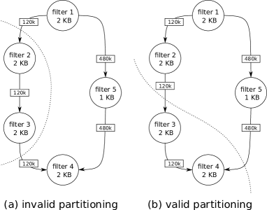
Figure 1: Subfigure (a) shows an invalid partition with minimal edge cut, but a bidirectional connection between blocks and thus a cycle in the quotient graph. A valid partitioning with minimal edge cut is shown in (b).

problem of mapping the nodes of a directed acyclic stream graph to the processors of an embedded multiprocessor. The nodes of the graph are kernels (small, self-contained functions) that are annotated with code size while edges are annotated with the amount of data that is transferred during one execution of the application.

The processors of the hardware platform have a private local data memory and a separate program memory. A direct memory access controller (DMA) is used to transfer data between the local memories and the external DDR memory of the system. Since the data memories only have a size in the order of hundreds of kilobytes they can only store a small portion of the image. Therefore the input image is divided into tiles. The mode of operation of this hardware usually is that the graph nodes are assigned to processors and process the tiles one after the other. However, this is only possible if the program memory size is sufficient to store all kernel programs. For the hardware platform under consideration it was found that this is not the case for more complex applications such as a Local Laplacian filter [24]. Therefore a gang scheduling [10] approach is used where the kernels are divided into groups of kernels (referred to as gangs) that do not violate memory constraints. Gangs are executed one after another on the hardware. After each execution, the kernels of the next gang are loaded. At no time any two kernels of different gangs are loaded in the program memories of the processors at the same time. Thus all intermediate data that is produced by the current gang but is needed by a kernel in a later gang needs to be transferred to external memory.

A strict ordering of gangs is required, because data can only be consumed in the same gang where it was produced and in gangs that are scheduled at a later point in time. If this does not hold, there is no valid temporal order in which the gangs can be executed on the platform. Such a partitioning is called acyclic because the quotient graph, which is created by contracting all nodes that are assigned to the same gang into a single node, does not contain a cycle for a valid acyclic partitioning. Figure 1 shows an example for an invalid and a valid partitioning.

Memory transfers, especially to external memories, are expensive in terms of power and time. Thus it is crucially important how the assignment of kernels to gangs is done, since it will affect the amount of data that needs to be transferred. In this work, we develop a multi-level approach to enhance our previous results.

3 Preliminaries

Basic Concepts.

Let $G=(V=\{0,\ldots,n-1\},E,c,\omega)$ be a directed graph with edge weights $\omega:E\to\mathbb{R}_{>0}$, node weights $c:V\to\mathbb{R}_{\geq 0}$, $n=|V|$, and $m=|E|$. We extend $c$ and $\omega$ to sets, i.e., $c(V^{\prime}):=\sum_{v\in V^{\prime}}c(v)$ and $\omega(E^{\prime}):=\sum_{e\in E^{\prime}}\omega(e)$. We are looking for blocks of nodes $V_{1}$,…,$V_{k}$ that partition $V$, i.e., $V_{1}\cup\cdots\cup V_{k}=V$ and $V_{i}\cap V_{j}=\emptyset$ for $i\neq j$. We call a block $V_{i}$ underloaded [overloaded] if $c(V_{i})<L_{\max}$ [if $c(V_{i})>L_{\max}$]. If a node $v$ has a neighbor in a block different of its own block then both nodes are called boundary nodes. An abstract view of the partitioned graph is the so-called quotient graph, in which nodes represent blocks and edges are induced by connectivity between blocks. The weighted version of the quotient graph has node weights which are set to the weight of the corresponding block and edge weights which are equal to the weight of the edges that run between the respective blocks.

A matching $M\subseteq E$ is a set of edges that do not share any common nodes, i.e., the graph $(V,M)$ has maximum degree one. Contracting an edge $(u,v)$ means to replace the nodes $u$ and $v$ by a new node $x$ connected to the former neighbors of $u$ and $v$, as well as connecting nodes that have $u$ and $v$ as neighbors to $x$. We set $c(x)=c(u)+c(v)$ so the weight of a node at each level is the number of nodes it is representing in the original graph. If replacing edges of the form $(u,w)$,$(v,w)$ would generate two parallel edges $(x,w)$, we insert a single edge with $\omega((x,w))=\omega((u,w))+\omega((v,w))$. Uncontracting an edge $e$ undoes its contraction. In order to avoid tedious notation, $G$ will denote the current state of the graph before and after a (un)contraction unless we explicitly want to refer to different states of the graph.

Problem Definition.

In our context, partitions have to satisfy two constraints: a balancing constraint and an acyclicity constraint. The balancing constraint demands that $\forall i\in\{1..k\}:c(V_{i})\leq L_{\max}:=(1+\epsilon)\lceil\frac{c(V)}{k}\rceil$ for some imbalance parameter $\epsilon\geq 0$. The acyclicity constraint mandates that the quotient graph is acyclic. The objective is to minimize the total edge cut $\sum_{i,j}w(E_{ij})$ where $E_{ij}:=\left\{(u,v)\in E\,:\,u\in V_{i},v\in V_{j}\right\}$. The directed graph partitioning problem with acyclic quotient graph (DGPAQ) is then defined as finding a partition $\varPi:=\left\{V_{1,}\ldots,V_{k}\right\}$ that satisfies both constraints while minimizing the objective function. In the undirected version of the problem the graph is undirected and no acyclicity constraint is given.

Multi-level Approach.

The multi-level approach to undirected graph partitioning consists of three main phases. In the contraction (coarsening) phase, the algorithm iteratively identifies matchings $M\subseteq E$ and contracts the edges in $M$. The result of the contraction is called a level. Contraction should quickly reduce the size of the input graph and each computed level should reflect the global structure of the input network. Contraction is stopped when the graph is small enough to be directly partitioned. In the refinement phase, the matchings are iteratively uncontracted. After uncontracting a matching, a refinement algorithm moves nodes between blocks in order to improve the cut size or balance. The intuition behind this approach is that a good partition at one level will also be a good partition on the next finer level, so local search converges quickly.

Relation to Scheduling.

Graph partitioning is a sub-step in our scheduling heuristic for the target hardware platform. We use a first pass of the graph partitioning heuristic with $L_{\max}$ set to the size of the program memory to find a good composition of kernels into programs with little interprocessor communication. The resulting quotient graph is then used in a second pass where $L_{\max}$ is set to the total number of processors in order to find scheduling gangs that minimize external memory transfers. In this second step the acyclicity constraint is crucially important. Note that in the first pass, the constraint can in principle be dropped. However, this yields programs with interdependencies that need to be scheduled in the same gang during the second pass. We found that this often leads to infeasible inputs for the second pass.

While the balancing constraint ensures that the size of the programs in a scheduling gang does not exceed the program memory size of the platform, reducing the edge cut will improve the memory bandwidth requirements of the application. The memory bandwidth is often the bottleneck, especially in embedded systems. A schedule that requires a large amount of transfers will neither yield a good throughput nor good energy efficiency [23]. However, in our previous work, we found that our graph partitioning heuristic while optimizing edge cut occasionally makes a bad decision concerning the composition of gangs. Ideally, the programs in a gang all have equal execution times. If one program runs considerably longer than the other programs, the corresponding processors will be idle since the context switch is synchronized. In this work, we try to alleviate this problem by using a fitness function in the evolutionary algorithm that considers the estimated execution times of the programs in a gang.

After partitioning, a schedule is generated for each gang. Since partitioning is the focus of this paper, we only give a brief outline. The scheduling heuristic is a single appearance list scheduler (SAS). In a SAS, the code of a function is never duplicated, in particular, a kernel will never execute on more than one processor. The reason for using a SAS is the scarce program memory. List schedulers iterate over a fixed priority list of programs and start the execution if the required input data and hardware resources for a program are available. We use a priority list sorted by the maximum length of the critical path which was calculated with estimated execution times. Since kernels perform mostly data-independent calculations, the execution time can be accurately predicted from the input size which is known from the stream graph and schedule.

Related Work.

There has been a vast amount of research on the undirected graph partitioning problem so that we refer the reader to [29, 3, 4] for most of the material. Here, we focus on issues closely related to our main contributions. All general-purpose methods for the undirected graph partitioning problem that are able to obtain good partitions for large real-world graphs are based on the multi-level principle. The basic idea can be traced back to multigrid solvers for systems of linear equations [30] but more recent practical methods are based on mostly graph theoretical aspects, in particular edge contraction and local search. For the undirected graph partitioning problem, there are many ways to create graph hierarchies such as matching-based schemes [32, 18, 25] or variations thereof [1] and techniques similar to algebraic multigrid, e.g. [20]. However, as node contraction in a DAG can introduce cycles, these methods can not be directly applied to the DAG partitioning problem. Well-known software packages for the undirected graph partitioning problem that are based on this approach include Jostle [32], KaHIP [27], Metis [18] and Scotch [7]. However, none of these tools can partition directed graphs under the constraint that the quotient graph is a DAG. Very recently, Hermann et al. [14] presented the first multi-level partitioner for DAGs. The algorithm finds matchings such that the contracted graph remains acyclic and uses an algorithm comparable to Fiduccia-Mattheyses algorithm [11] for refinement. Neither the code nor detailed results per instance are available at the moment.

Gang scheduling was originally introduced to efficiently schedule parallel programs with fine-grained interactions [10]. In recent work, this concept has been applied to schedule parallel applications on virtual machines in cloud computing [31] and extended to include hard real-time tasks [12]. An important difference to our work is that in gang scheduling all tasks that exchange data with each other are assigned to the same gang, thus there is no communication between gangs. In our work, the limited program memory of embedded platforms does not allow to assign all kernels to the same gang. Therefore, there is communication between gangs which we aim to minimize by employing graph partitioning methods.

Another application area for graph partitioning algorithms that does have a constraint on cyclicity is the temporal partitioning in the context of reconfigurable hardware like field-programmable gate arrays (FPGAs). These are processors with programmable logic blocks that can be reprogramed and rewired by the user. In the case where the user wants to realize a circuit design that exceeds the physical capacities of the FPGA, the circuit netlist needs to be partitioned into partial configurations that will be realized and executed one after another. The first algorithms for temporal partitioning worked on circuit netlists expressed as hypergraphs. Now, algorithms usually work on a behavioral level expressed as a regular directed graph. The proposed algorithms include list scheduling heuristics [5] or are based on graph-theoretic theorems like max-flow min-cut [16], with objective functions ranging from minimizing the communication cost incurred by the partitioning [5, 16] to reducing the length of the critical path in a partition [5, 17]. Due to the different nature of the problem and different objectives, a direct comparison with these approaches is not possible.

The algorithm proposed in [6] partitions a directed, acyclic dataflow graph under acyclicity constraints while minimizing buffer sizes. The authors propose an optimal algorithm with exponential complexity that becomes infeasible for larger graphs and a heuristic which iterates over perturbations of a topological order. The latter is comparable to our initial partitioning and our first refinement algorithm. We see in the evaluation that moving to a multi-level and evolutionary algorithm clearly outperforms this approach. Note that minimizing buffer sizes is not part of our objective.

4 Multi-level Approach to Acyclic Graph Partitioning

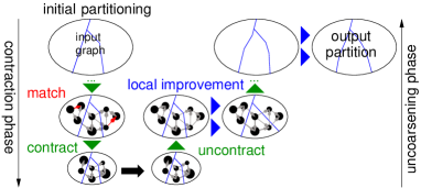
Figure 2: The multi-level approach to graph partitioning.

Multi-level techniques have been widely used in the field of graph partitioning for undirected graphs. We now transfer the techniques used in the KaFFPa multi-level algorithm [27] to a new algorithm that is able to tackle the DAG partitioning problem. More precisely, to obtain a multi-level DAG partitioning algorithm, we integrate local search algorithms that keep the quotient graph acyclic and handle problems that occur when coarsening a DAG.

Before we give an in-depth description, we present an overview of the algorithm (see also Figure 2). Recall that a multi-level graph partitioner has three phases: coarsening, initial partitioning and uncoarsening. In contrast to classic multi-level algorithms, our algorithm starts to construct a solution on the finest level of the hierarchy and not with the coarsening phase. This is necessary, since contracting matchings can create coarser graphs that contain cycles, and hence it may become impossible to find feasible solutions on the coarsest level of the hierarchy. After initial partitioning of the graph, we continue to coarsen the graph until it has no matchable edges left. During coarsening, we transfer the solution from the finest level through the hierarchy and use it as initial partition on the coarsest graph. As we will see later, since the partition on the finest level has been feasible, i.e. acyclic and balanced, so will be the partition that we transferred to the coarsest level. The coarser versions of the input graph may still contain cycles, but local search maintains feasibility on each level and hence, after uncoarsening is done, we obtain a feasible solution on the finest level. The rest of the section is organized as follows. We begin by reviewing the construction algorithm that we use, continue with the description of the coarsening phase and then recap local search algorithms for the DAG partitioning problem that are now used within the multi-level approach.

4.1 Initial Partitioning

Recall that our algorithm starts with initial partitioning on the finest level of the hierarchy. Our initial partitioning algorithm [22], creates an initial solution based on a topological ordering of the input graph and then applies a local search strategy to improve the objective of the solution while maintaining both constraints – balance and acyclicity.

More precisely, the initial partitioning algorithm computes a random topological ordering of nodes using a modified version of Kahn’s algorithm with randomized tie-breaking. The algorithm maintains a list $S$ with all nodes that have indegree zero and an initially empty list $T$. It then repeatedly removes a random node $n$ from list $S$, removes $n$ from the graph, updates $S$ by potentially adding further nodes with indegree zero and adds $n$ to the tail of $T$. Using list $T$, we can now derive initial solutions by dividing the graph into blocks of consecutive nodes w.r.t to the ordering. Due to the properties of the topological ordering, there is no node in a block $V_{j}$ that has an outgoing edge ending in a block $V_{i}$ with $i<j$. Hence, the quotient graph of the solution is cycle-free. In addition, the blocks are chosen such that the balance constraint is fulfilled. The initial solution is then improved by applying a local search algorithm. Since the construction algorithm is randomized, we run the heuristics multiple times using different random seeds and pick the best solution afterwards. We call this algorithm single-level algorithm.

4.2 Coarsening

Our coarsening algorithm makes contraction more systematic by separating two issues [27]: A rating function indicates how much sense it makes to contract an edge based on local information. A matching algorithm tries to maximize the summed ratings of the contracted edges by looking at the global structure of the graph. While the rating function allows a flexible characterization of what a “good” contracted graph is, the simple, standard definition of the matching problem allows to reuse previously developed algorithms for weighted matching. Matchings are contracted until the graph is “small enough”. In [15], the rating function $\mathrm{expansion}^{*2}(u,v):=\frac{\omega(u,v)^{2}}{c(u)c(v)}$ works best among other edge rating functions, so that we also use this rating function for the DAG partitioning problem.

As in KaFFPa [27], we employ the Global Path Algorithm (GPA) as a matching algorithm. We apply the matching algorithm on the undirected graph that is obtained by interpreting each edge in the DAG as undirected edge without introducing parallel edges. The GPA algorithm was proposed by Maue and Sanders [19] as a synthesis of the Greedy algorithm and the Path Growing Algorithm [9]. This algorithm achieves a half-approximation in the worst case, but empirically, GPA gives considerably better results than Sorted Heavy Edge Matching and Greedy (for more details see [15]). The GPA algorithm scans the edges in order of decreasing weight but rather than immediately building a matching, it first constructs a collection of paths and even cycles, and for each of those computes optimal solutions.

Recall that our algorithm starts with a partition on the finest level of the hierarchy. Hence, we set cut edges not to be eligible for the matching algorithm. This way edges that run between blocks of the given partition are not contracted. Thus the given partition can be used as a feasible initial partition of the coarsest graph. The partition on the coarsest level has the same balance and cut as the input partition. Additionally, it is also an acyclic partition of the coarsest graph. Performing coarsening by this method ensures non-decreasing partition quality, if the local search algorithm guarantees no worsening. Moreover, this allows us to use standard weighted matching algorithms, instead of using more restricted matching algorithms that ensure that the contracted graph is also a DAG. We stop contraction when no matchable edge is left.

4.3 Local Search

Recall that the refinement phase iteratively uncontracts the matchings contracted during the first phase. Due to the way contraction is defined, a partitioning of the coarse level creates a partitioning of the finer graph with the same objective and balance, moreover, it also maintains the acyclicity constraint on the quotient graph. After a matching is uncontracted, local search refinement algorithms move nodes between block boundaries in order to improve the objective while maintaining the balancing and acyclicity constraint. We use the local search algorithms of Moreira et al. [22]. We give an indepth description of the algorithms in Appendix 0.A and shortly outline them here. All algorithms identify movable nodes which can be moved to other blocks without violating any of the constraints. Based on a topological ordering, the first algorithm uses a sufficient condition which can be evaluated quickly to check the acyclicity constraint. Since the first heuristic can miss possible moves by solely relying upon a sufficient condition, the second heuristic [22] maintains a quotient graph during all iterations and uses Kahn’s algorithm to check whether a move creates a cycle in it. The third heuristic combines the quick check for acyclicity of the first heuristic with an adapted Fiduccia-Mattheyses algorithm [11] which gives the heuristic the ability to climb out of a local minimum.

5 Evolutionary Components

Evolutionary algorithms start with a population of individuals, in our case partitions of the graph, which are created by our multi-level algorithm using different random seeds. It then evolves the population into different populations over several rounds using recombination and mutation operations. In each round, the evolutionary algorithm uses a two-way tournament selection rule [21] based on the fitness of the individuals of the population to select good individuals for recombination or mutation. Here, the fittest out of two distinct random individuals from the population is selected. We focus on a simple evolutionary scheme and generate one offspring per generation. When an offspring is generated, we use an eviction rule to select a member of the population and replace it with the new offspring. In general, one has to take both, the fitness of an individual and the distance between individuals in the population, into consideration [2]. We evict the solution that is most similar to the offspring among those individuals in the population that have a cut worse or equal to the cut of the offspring itself. The difference of two individuals is defined as the size of the symmetric difference between their sets of cut edges.

We now explain our multi-level recombine and mutation operators. Our recombine operator ensures that the partition quality, i.e. the edge cut, of the offspring is at least as good as the best of both parents. For our recombine operator, let $\mathcal{P}_{1}$ and $\mathcal{P}_{2}$ be two individuals from the population. Both individuals are used as input for our multi-level DAG partitioning algorithm in the following sense. Let $\mathcal{E}$ be the set of edges that are cut edges, i.e. edges that run between two blocks, in either $\mathcal{P}_{1}$ or $\mathcal{P}_{2}$. All edges in $\mathcal{E}$ are blocked during the coarsening phase, i.e. they are not contracted during the coarsening phase. In other words, these edges are not eligible for the matching algorithm used during the coarsening phase and therefore are not part of any matching computed. As before, the coarsening phase of the multi-level scheme stops when no contractable edge is left. As soon as the coarsening phase is stopped, we apply the better out of both input partitions w.r.t to the objective to the coarsest graph and use this as initial partitioning. We use random tie-breaking if both input individuals have the same objective value. This is possible since we did not contract any cut edge of $\mathcal{P}$. Again, due to the way coarsening is defined, this yields a feasible partition for the coarsest graph that fulfills both constraints (acyclicity and balance) if the input individuals fulfill those.

Note that due to the specialized coarsening phase and specialized initial partitioning, we obtain a high quality initial solution on a very coarse graph. Since our local search algorithms guarantee no worsening of the input partition and use random tie breaking, we can assure nondecreasing partition quality. Also note that local search algorithms can effectively exchange good parts of the solution on the coarse levels by moving only a few nodes. Due to the fact that our multi-level algorithms are randomized, a recombine operation performed twice using the same parents can yield a different offspring. Each time we perform a recombine operation, we choose one of the local search algorithms described in Section 4.3 uniformly at random.

Cross Recombine.

This operator recombines an individual of the population with a partition of the graph that can be from a different problem space, e.g. a $k^{\prime}$-partition of the graph. While $\mathcal{P}_{1}$ is chosen using tournament selection as before, we create $\mathcal{P}_{2}$ in the following way. We choose $k^{\prime}$ uniformly at random in $[k/4,4k]$ and $\epsilon^{\prime}$ uniformly at random in $[\epsilon,4\epsilon]$. We then create $\mathcal{P}_{2}$ (a $k^{\prime}$-partition with a relaxed balance constraint) by using the multi-level approach. The intuition behind this is that larger imbalances reduce the cut of a partition and using a $k^{\prime}$-partition instead of $k$ may help us to discover cuts in the graph that otherwise are hard to discover. Hence, this yields good input partitions for our recombine operation.

Mutation.

We define two mutation operators. Both mutation operators use a random individual $\mathcal{P}_{1}$ from the current population. The first operator starts by creating a $k$-partition $\mathcal{P}_{2}$ using the multi-level scheme. It then performs a recombine operation as described above, but not using the better of both partitions on the coarsest level, but $\mathcal{P}_{2}$. The second operator ensures nondecreasing quality. It basically recombines $\mathcal{P}_{1}$ with itself (by setting $\mathcal{P}_{2}=\mathcal{P}_{1}$). In both cases, the resulting offspring is inserted into the population using the eviction strategy described above.

Fitness Function.

Recall that the execution of programs in a gang is synchronized. Therefore, a lower bound on the gang execution time is given by the longest execution time of a program in a gang. Pairing programs with short execution times with a single long-running program leads to a bad utilization of processors, since the processors assigned to the short-running programs are idle until all programs have finished. To avoid these situations, we use a fitness function that estimates the critical path length of the entire application by identifying the longest-running programs per gang and summing their execution times. This will result in gangs, where long-running programs are paired with other long-running programs. More precisely, the input graph is annotated with execution times for each node that were obtained by profiling the corresponding kernels on our target hardware. The execution time of a program is calculated by accumulating the execution times for all firings of its contained kernels. The quality of a solution to the partitioning problem is then measured by the fitness function which is a linear combination of the obtained edge cut and the critical path length. Note, however, that the recombine and mutation operations still optimize for cuts.

Miscellanea.

We follow the parallelization approach of [28]: Each processing element (PE) has its own population and performs the same operations using different random seeds. The parallelization / communication protocol is similar to randomized rumor spreading [8]. We follow the description of [28] closely: A communication step is organized in rounds. In each round, a PE chooses a communication partner uniformly at random among those who did not yet receive $P$ and sends the current best partition $P$ of the local population. Afterwards, a PE checks if there are incoming individuals and if so inserts them into the local population using the eviction strategy described above. If $P$ is improved, all PEs are again eligible.

6 Experimental Evaluation

System.

We have implemented the algorithms described above within the KaHIP [27] framework using C++. All programs have been compiled using g++ 4.8.0 with full optimizations turned on (-O3 flag) and 32 bit index data types. We use two machines for our experiments: machine A has two Octa-Core Intel Xeon E5-2670 processors running at 2.6 GHz with 64 GB of local memory. We use this machine in Section 6.1. Machine B is equipped with two Intel Xeon X5670 Hexa-Core processors (Westmere) running at a clock speed of 2.93 GHz. The machine has 128 GB main memory, 12 MB L3-Cache and 6$\times$256 KB L2-Cache. We use this machine in Section 6.2. Henceforth, a PE is one core.

Methodology.

We mostly present two kinds of data: average values and plots that show the evolution of solution quality (convergence plots). In both cases we perform multiple repetitions. The number of repetitions is dependent on the test that we perform. Average values over multiple instances are obtained as follows: for each instance (graph, $k$), we compute the geometric mean of the average edge cut for each instance. We now explain how we compute the convergence plots, starting with how they are computed for a single instance $I$: whenever a PE creates a partition, it reports a pair ($t$, cut) where the timestamp $t$ is the current elapsed time on the particular PE and cut refers to the cut of the partition that has been created. When performing multiple repetitions, we report average values ($\overline{t}$, avgcut) instead. After completion of the algorithm, we have $P$ sequences of pairs ($t$, cut) which we now merge into one sequence. The merged sequence is sorted by the timestamp $t$. The resulting sequence is called $T^{I}$. Since we are interested in the evolution of the solution quality, we compute another sequence $T^{I}_{\text{min}}$. For each entry (in sorted order) in $T^{I}$ we insert the entry $(t,\min_{t^{\prime}\leq t}\text{cut}(t^{\prime}))$ into $T^{I}_{\text{min}}$. Here $\min_{t^{\prime}\leq t}\text{cut}(t^{\prime})$ is the minimum cut that occurred until time $t$. $N^{I}_{\text{min}}$ refers to the normalized sequence, i.e. each entry ($t$, cut) in $T^{I}_{\text{min}}$ is replaced by ($t_{n}$, cut) where $t_{n}=t/t_{I}$ and $t_{I}$ is the average time that the multi-level algorithm needs to compute a partition for the instance $I$. To obtain average values over multiple instances we do the following: for each instance we label all entries in $N^{I}_{\text{min}}$, i.e. ($t_{n}$, cut) is replaced by ($t_{n}$, cut, $I$). We then merge all sequences $N^{I}_{\text{min}}$ and sort by $t_{n}$. The resulting sequence is called $S$. The final sequence $S_{g}$ presents event based geometric averages values. We start by computing the geometric mean cut value $\mathcal{G}$ using the first value of all $N^{I}_{\text{min}}$ (over $I$). To obtain $S_{g}$, we sweep through $S$: for each entry (in sorted order) $(t_{n},c,I)$ in $S$ we update $\mathcal{G}$, i.e. the cut value of $I$ that took part in the computation of $\mathcal{G}$ is replaced by the new value $c$, and insert $(t_{n},\mathcal{G})$ into $S_{g}$. Note that $c$ can be only smaller or equal to the old cut value of $I$.

Instances.

We use the algorithms under consideration on a set of instances from the Polyhedral Benchmark suite (PolyBench) [26] which have been kindly provided by Hermann et al. [14]. In addition, we use an instance of Moreira [22]. Basic properties of the instances can be found in Appendix Table 2.

6.1 Evolutionary DAG Partitioning with Cut as Objective

We will now compare the different proposed algorithms. Our main objective in this section is the cut objective. In our experiments, we use the imbalance parameter $\epsilon=3\%$. We use 16 PEs of machine A and two hours of time per instance when we use the evolutionary algorithm. We parallelized repeated executions of multi- and single-level algorithms since they are embarrassingly parallel for different seeds and also gave 16 PEs and two hours of time to each of the algorithms. Each call of the multi-level and single-level algorithm uses one of our local search algorithms at random and a different random seed. We look at $k\in\{2,4,8,16,32\}$ and performed three repetitions per instance. Figure 3 shows convergence and performance plots and Tables 3, 4 in the Appendix show detailed results per instance. To get a visual impression of the solution quality of the different algorithms, Figure 3 also presents a performance plot using all instances (graph, $k$). A curve in a performance plot for algorithm X is obtained as follows: For each instance, we calculate the ratio between the best cut obtained by any of the considered algorithms and the cut for algorithm X. These values are then sorted.

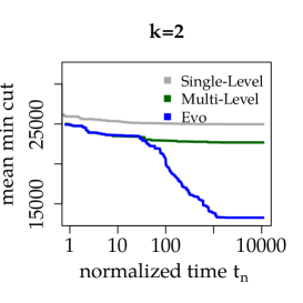
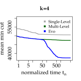
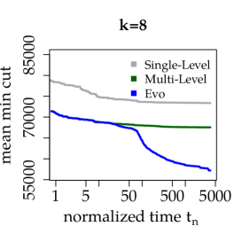
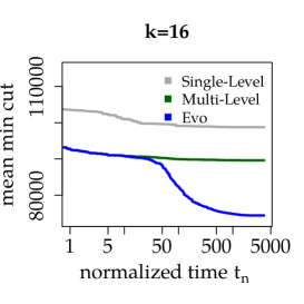
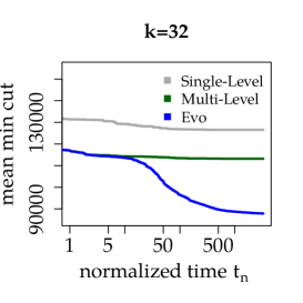
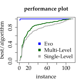
Figure 3: Convergence plots for $k\in\{2,4,8,16,32\}$ and a performance plot.

First of all, the performance plot in Figure 3 indicates that our evolutionary algorithm finds significantly smaller cuts than the single- and multi-level scheme. Using the multi-level scheme instead of the single-level scheme already improves the result by 10% on average. This is expected since using the multi-level scheme introduces a more global view to the optimization problem and the multi-level algorithm starts from a partition created by the single-level algorithm (initialization algorithm + local search). In addition, the evolutionary algorithm always computes a better result than the single-level algorithm. This is true for the average values of the repeated runs as well as the achieved best cuts. The single-level algorithm computes average cuts that are 42% larger than the ones computed by the evolutionary algorithm and best cuts that are 47% larger than the best cuts computed by the evolutionary algorithm. As anticipated, the evolutionary algorithm computes the best result in almost all cases. In three cases the best cut is equal to the multi-level, and in three other cases the result of the multi-level algorithm is better (at most 3%, e.g. for $k=2$, covariance). These results are due to the fact that we already use the multi-level algorithm to initialize the population of the evolutionary algorithm. In addition, after the initial population is built, the recombine and mutation operations can successfully improve the solutions in the population further and break out of local minima (see Figure 3). Average cuts of the evolutionary algorithm

$k$	Single-Level	Multi-Level
2	112%	89%
4	34%	23%
8	28%	18%
16	32%	20%
32	44%	28%

Table 1: Average increase of best cuts over best cuts of evolutionary algorithm.

are 29% smaller than the average cuts computed by the multi-level algorithm (and 33% in case of best cuts). The largest improvement of the evolutionary algorithm over the single- and multi-level algorithm is a factor 39 (for $k=2$, 3mm0). Table 1 shows how improvements are distributed over different values of $k$. Interestingly, in contrast to evolutionary algorithms for the undirected graph partitioning problem, e.g. [28], improvements to the multi-level algorithm do not increase with increasing $k$. Instead, improvements more diversely spread over different values of $k$. We believe that the good performance of the evolutionary algorithm is due to a very fragmented search space that causes local search heuristics to easily get trapped in local minima, especially since local search algorithms maintain the feasibility on the acyclicity constraint. Due to mutation and recombine operations, our evolutionary algorithm escapes those more effectively than the multi- or single-level approach.

6.2 Impact on Imaging Application

We evaluate the impact of the improved partitioning heuristic on an advanced imaging algorithm, the Local Laplacian filter. The Local Laplacian filter is an edge-aware image processing filter. The algorithm uses the concepts of Gaussian pyramids and Laplacian pyramids as well as a point-wise remapping function to enhance image details without creating artifacts. A detailed description of the algorithm and theoretical background is given in [24]. We model the dataflow of the filter as a DAG where nodes are annotated with the program size and an execution time estimate and edges with the corresponding data transfer size. The DAG has $489$ nodes and $631$ edges in total in our configuration. We use all algorithms (multi-level, evolutionary), the evolutionary with the fitness function set to the one described in Section 5. We compare our algorithms with the best local search heuristic from our previous work [22] The time budget given to each heuristic is ten minutes. The makespans for each resulting schedule are obtained with a cycle-true compiled simulator of the hardware platform. We vary the available bandwidth to external memory to assess the impact of edge cut on schedule makespan. In the following, a bandwidth of $x$ refers to $x$ times the bandwidth available on the real hardware. The relative improvement in makespan is compared to our previous heuristic in [22].

In this experiment, the results in terms of edge cut as well as makespan are similar for the multi-level and the evolutionary algorithm optimizing for cuts, as the filter is fairly small. However, the new approaches improve the makespan of the application. This is mainly because the reduction of the edge cut reduces the amount of data that needs to be transferred to external memories. Improvements range from 1% to 5% depending on the available memory bandwidth with high improvements being seen for small memory bandwidths. For larger memory bandwidths, the improvement in makespan diminishes since the pure reduction of communication volume becomes less important. Using our new fitness function that incorporates critical path length increases the makespan by 40% to 10% if the memory bandwidth is scarce (for bandwidths ranging from 1 to 3). We found that the gangs in this case are almost always memory-limited and thus reducing communication volume is predominantly important. With more bandwidth available, including critical path length in the fitness function improves the makespan by 3% to 33% for bandwidths ranging from 4 to 10. Hence, using the fitness function results in a convenient way to fine-tune the heuristic for a given memory bandwidth. For hardware platforms with a scarce bandwidth, reducing the edge cut is the best. If more bandwidth is available, for example if more than one DMA engine is available, one can change the factors of the linear combination to gradually reduce the impact of edge cut in favor of critical path length.

7 Conclusion

Directed graphs are widely used to model data flow and execution dependencies in streaming applications which enables the utilization of graph partitioning algorithms for the problem of parallelizing computation for multiprocessor architectures. In this work, we introduced a novel multi-level algorithm as well as the first evolutionary algorithm for the acyclic graph partitioning problem. Additionally, we formulated an objective function that improves load balancing on the target platform which is then used as fitness function in the evolutionary algorithm. Extensive experiments over a large set of graphs and a real application indicate that the multi-level as well as the evolutionary algorithm significantly improve the state-of-the-art. Our experiments indicate that the search space has many local minima. Hence, in future work, we want to experiment with relaxed constraints on coarser levels of the hierarchy. Other future directions of research include multi-level algorithms that directly optimize the newly introduced fitness function.

Appendix 0.A Details on Local Search Algorithms

The first heuristic identifies movable nodes which can be moved to other blocks without violating the constraints. It uses a sufficient condition to check the acyclicity constraint. Since the acyclicity constraint was maintained by the previous steps, a topological ordering of blocks exists such that all edges between blocks are forward edges w.r.t. to the ordering. Moving a node from one block to another can potentially turn a forward edge into a back edge. To ensure acyclicity, it is sufficient to avoid these moves since only then the original ordering of blocks will remain intact. This condition can be checked very fast for a node $v\in V_{i}$. All incoming edges are checked to find the node $u\in V_{A}$ where $A$ is maximal. $A\leq i$ must hold, otherwise the topological ordering already contains a back edge. If $A<i$, then the node can be moved to blocks preceding $V_{i}$ up to and including $V_{A}$ in the topological ordering without creating a back edge. This is because all incoming edges of the node will either be internal to block $V_{A}$ or are forward edges starting from blocks preceding $V_{A}$. The same reasoning can be made for outgoing edges of $v$ to identify block succeeding $V_{i}$ that are eligible for a move. After finding all movable nodes under this condition, the heuristic will choose the move with the highest gain. The complexity of this heuristic is $O(m)$ [22].

Since the first heuristic can miss possible moves by solely relying upon a sufficient condition, the second heuristic [22] maintains a quotient graph during all iterations and uses Kahn’s algorithm to check whether a cycle was created whenever a move causes a new edge to appear in the quotient graph and the sufficient condition does not give an answer. The cost is $O(km)$ if the quotient graph is sparse.

The third heuristic combines the quick check for acyclicity of the first heuristic with an adapted Fiduccia-Mattheyses algorithm [11] which gives the heuristic the ability to climb out of a local minimum. The initial partitioning is improved by exchanging nodes between a pair of blocks. The algorithm will then calculate the gain for all movable nodes and insert them into a priority queue. Moves with highest gains are committed if they do not overload the target block. After each move, it is checked whether a former internal node in block is now an boundary node, if so, the gain for this node is calculated and it is inserted into the priority queue. Similarly, a node that previously was movable might now be locked in its block. In this case, the node will be marked as locked since searching and deleting the node in the priority queue has a much higher computational complexity.

The inner pass of the heuristic stops when the priority queue is depleted or after $2n/k$ moves which did not have a measurable impact on the quality of obtained partitionings. The solution with best objective that was achieved during the pass will be returned. The outer pass of the heuristic will repeat the inner pass for randomly chosen pairs of blocks. At least one of these blocks has to be “active”. Initially, all blocks are marked as “active”. If and only if the inner pass results in movement of nodes, the two blocks will be marked as active for the next iteration. The heuristic stops if there are no more active blocks. The complexity is $O(m+n\log\frac{n}{k})$ if the quotient graph is sparse.

Appendix 0.B Basic Instance Properties

Graph	$n$	$m$	Graph	$n$	$m$
2mm0	36 500	62 200	atax	241 730	385 960
syr2k	111 000	180 900	symm	254 020	440 400
3mm0	111 900	214 600	fdtd-2d	256 479	436 580
doitgen	123 400	237 000	seidel-2d	261 520	490 960
durbin	126 246	250 993	trmm	294 570	571 200
jacobi-2d	157 808	282 240	heat-3d	308 480	491 520
gemver	159 480	259 440	lu	344 520	676 240
covariance	191 600	368 775	ludcmp	357 320	701 680
mvt	200 800	320 000	gesummv	376 000	500 500
jacobi-1d	239 202	398 000	syrk	594 480	975 240
trisolv	240 600	320 000	adi	596 695	1 059 590
gemm	1 026 800	1 684 200

Table 2: Basic properties of the our benchmark instances.

Appendix 0.C Detailed per Instance Results

		Evolutionary Algorithm			Multi-Level Algorithm			Single-Level Algorithm
graph	$k$	Avg. Cut	Best Cut	Balance	Avg. Cut	Best Cut	Balance	Avg. Cut	Best Cut	Balance
2mm0	2	200	200	1.00	200	200	1.00	400	400	1.02
2mm0	4	947	930	1.03	9 167	9 089	1.03	12 590	12 533	1.03
2mm0	8	7 181	6 604	1.03	17 445	17 374	1.03	20 259	20 231	1.03
2mm0	16	13 330	13 092	1.03	22 196	22 125	1.00	25 671	25 591	1.03
2mm0	32	14 583	14 321	1.02	25 178	24 962	1.00	29 237	29 209	1.03
3mm0	2	1 000	1 000	1.01	39 069	39 053	1.03	39 057	39 055	1.03
3mm0	4	38 722	37 899	1.03	56 109	54 192	1.03	60 795	60 007	1.03
3mm0	8	58 129	49 559	1.03	83 225	83 006	1.03	90 627	90 449	1.03
3mm0	16	64 384	60 127	1.03	95 052	94 761	1.03	105 627	105 122	1.03
3mm0	32	62 279	58 190	1.03	103 344	103 314	1.03	115 138	114 853	1.03
adi	2	134 945	134 675	1.03	155 232	155 232	1.02	158 115	158 058	1.00
adi	4	284 666	283 892	1.03	286 673	276 213	1.02	298 392	298 355	1.03
adi	8	290 823	290 672	1.03	296 728	296 682	1.03	309 067	308 651	1.03
adi	16	326 963	326 923	1.03	335 778	335 373	1.03	366 073	362 382	1.03
adi	32	370 876	370 413	1.03	378 883	378 572	1.03	413 394	413 138	1.03
atax	2	47 826	47 424	1.03	48 302	48 302	1.00	61 425	60 533	1.03
atax	4	82 397	76 245	1.03	112 616	111 295	1.03	116 183	115 807	1.03
atax	8	113 410	111 051	1.03	129 373	129 169	1.03	144 918	144 614	1.03
atax	16	127 687	125 146	1.03	141 709	141 052	1.03	157 799	157 541	1.03
atax	32	132 092	130 854	1.03	147 416	147 028	1.03	167 963	167 756	1.03
covariance	2	66 520	66 445	1.03	66 432	66 365	1.03	67 534	67 450	1.03
covariance	4	84 626	84 213	1.03	90 582	90 170	1.03	95 801	95 676	1.03
covariance	8	103 710	102 425	1.03	110 996	109 307	1.03	122 410	122 017	1.03
covariance	16	125 816	123 276	1.03	141 706	141 142	1.03	155 390	154 446	1.03
covariance	32	142 214	137 905	1.03	168 378	167 678	1.03	173 512	173 275	1.03
doitgen	2	43 807	42 208	1.03	58 218	58 123	1.03	58 216	58 190	1.03
doitgen	4	72 115	71 072	1.03	83 422	83 278	1.03	85 531	85 279	1.03
doitgen	8	76 977	75 114	1.03	98 418	98 234	1.03	105 182	105 027	1.03
doitgen	16	84 203	77 436	1.03	107 795	107 720	1.03	115 506	115 152	1.03
doitgen	32	94 135	92 739	1.03	114 439	114 241	1.03	124 564	124 457	1.03
durbin	2	12 997	12 997	1.02	13 203	13 203	1.00	13 203	13 203	1.00
durbin	4	21 641	21 641	1.02	21 724	21 720	1.00	21 732	21 730	1.00
durbin	8	27 571	27 571	1.01	27 650	27 647	1.01	27 668	27 666	1.01
durbin	16	32 865	32 865	1.03	33 065	33 045	1.03	33 340	33 329	1.03
durbin	32	39 726	39 725	1.03	40 481	40 457	1.03	41 204	41 178	1.03
fdtd-2d	2	5 494	5 494	1.01	5 966	5 946	1.01	6 437	6 427	1.00
fdtd-2d	4	15 100	15 099	1.03	16 948	16 893	1.02	18 210	18 170	1.00
fdtd-2d	8	33 087	32 355	1.03	38 767	38 687	1.03	41 267	41 229	1.01
fdtd-2d	16	35 714	35 239	1.02	78 458	78 311	1.03	83 498	83 437	1.03
fdtd-2d	32	43 961	42 507	1.02	106 003	105 885	1.03	128 443	128 146	1.03
gemm	2	383 084	382 433	1.03	384 778	384 490	1.03	388 243	387 685	1.03
gemm	4	507 250	500 526	1.03	532 558	531 419	1.03	555 800	555 541	1.03
gemm	8	578 951	575 004	1.03	611 551	609 528	1.03	649 641	647 955	1.03
gemm	16	615 342	613 373	1.03	658 565	654 826	1.03	701 624	699 215	1.03
gemm	32	626 472	623 271	1.03	703 613	701 886	1.03	751 441	750 144	1.03
gemver	2	29 349	29 270	1.03	31 482	31 430	1.03	32 785	32 718	1.03
gemver	4	49 361	49 229	1.03	54 884	54 683	1.03	58 920	58 886	1.03
gemver	8	68 163	67 094	1.03	74 114	74 005	1.03	82 140	81 935	1.03
gemver	16	78 115	75 596	1.03	86 623	86 476	1.02	98 061	97 851	1.03
gemver	32	85 331	84 865	1.03	94 574	94 295	1.02	110 439	110 250	1.03
gesummv	2	1 666	500	1.02	61 764	61 404	1.03	102 406	101 530	1.01
gesummv	4	98 542	94 493	1.02	109 121	108 200	1.00	135 352	134 783	1.03
gesummv	8	101 533	98 982	1.01	116 534	116 167	1.01	159 982	159 456	1.03
gesummv	16	112 064	104 866	1.03	123 615	121 960	1.02	184 950	184 645	1.03
gesummv	32	117 752	114 812	1.03	135 491	133 445	1.03	195 511	195 483	1.03

Table 3: Detailed per Instance Results

		Evolutionary Algorithm			Multi-Level Algorithm			Single-Level Algorithm
graph	$k$	Avg. Cut	Best Cut	Balance	Avg. Cut	Best Cut	Balance	Avg. Cut	Best Cut	Balance
heat-3d	2	8 695	8 684	1.01	8 997	8 975	1.01	9 136	9 100	1.01
heat-3d	4	14 592	14 592	1.01	16 150	16 092	1.02	16 639	16 602	1.02
heat-3d	8	20 608	20 608	1.02	24 869	24 787	1.03	26 072	26 024	1.03
heat-3d	16	31 615	31 500	1.03	41 120	41 049	1.03	43 434	43 323	1.03
heat-3d	32	51 963	50 758	1.03	70 598	70 524	1.03	78 086	77 888	1.03
jacobi-1d	2	596	596	1.01	656	652	1.00	732	729	1.00
jacobi-1d	4	1 493	1 492	1.01	1 739	1 736	1.00	1 994	1 990	1.00
jacobi-1d	8	3 136	3 136	1.01	3 811	3 803	1.00	4 398	4 392	1.00
jacobi-1d	16	6 340	6 338	1.01	7 884	7 880	1.00	9 161	9 159	1.00
jacobi-1d	32	8 923	8 750	1.03	15 989	15 987	1.02	18 613	18 602	1.01
jacobi-2d	2	2 994	2 991	1.02	3 227	3 223	1.01	3 573	3 568	1.01
jacobi-2d	4	5 701	5 700	1.02	6 771	6 749	1.01	7 808	7 797	1.01
jacobi-2d	8	9 417	9 416	1.03	12 287	12 160	1.03	14 714	14 699	1.03
jacobi-2d	16	16 274	16 231	1.03	23 070	22 971	1.03	27 943	27 860	1.03
jacobi-2d	32	22 181	21 758	1.03	43 956	43 928	1.03	52 988	52 969	1.03
lu	2	5 210	5 162	1.03	5 183	5 174	1.03	5 184	5 173	1.03
lu	4	13 528	13 510	1.03	14 160	14 122	1.03	14 220	14 189	1.03
lu	8	33 307	33 211	1.03	33 890	33 764	1.03	33 722	33 625	1.03
lu	16	74 543	74 006	1.03	76 399	75 043	1.03	78 698	78 165	1.03
lu	32	130 674	129 954	1.03	143 735	143 396	1.03	151 452	150 549	1.02
ludcmp	2	5 380	5 337	1.02	5 337	5 337	1.02	5 337	5 337	1.02
ludcmp	4	14 744	14 744	1.03	17 352	17 278	1.03	17 322	17 252	1.03
ludcmp	8	37 228	37 069	1.03	40 579	40 420	1.03	40 164	39 752	1.03
ludcmp	16	78 646	78 467	1.03	81 951	81 778	1.03	85 882	85 582	1.03
ludcmp	32	134 758	134 288	1.03	150 112	149 930	1.03	157 788	156 570	1.03
mvt	2	24 528	23 091	1.02	63 485	63 054	1.03	80 468	80 408	1.03
mvt	4	74 386	73 035	1.02	83 951	82 868	1.03	102 122	101 359	1.03
mvt	8	86 525	82 221	1.03	96 695	96 362	1.01	116 068	115 722	1.03
mvt	16	99 144	97 941	1.03	107 347	107 032	1.01	129 178	128 962	1.03
mvt	32	105 066	104 917	1.03	115 123	114 845	1.01	143 436	143 205	1.03
seidel-2d	2	4 991	4 969	1.01	5 441	5 384	1.00	5 461	5 397	1.00
seidel-2d	4	12 197	12 169	1.01	13 358	13 334	1.01	13 387	13 372	1.01
seidel-2d	8	21 419	21 400	1.01	24 011	23 958	1.02	24 167	24 150	1.01
seidel-2d	16	38 222	38 110	1.02	43 169	43 071	1.02	43 500	43 419	1.02
seidel-2d	32	52 246	51 531	1.03	79 882	79 813	1.03	81 433	81 077	1.03
symm	2	94 357	94 214	1.03	95 630	95 429	1.03	96 934	96 765	1.03
symm	4	127 497	126 207	1.03	134 923	134 888	1.03	149 064	148 653	1.03
symm	8	152 984	151 168	1.03	161 622	161 575	1.03	175 299	175 169	1.03
symm	16	167 822	167 512	1.03	177 001	176 568	1.03	190 628	190 519	1.03
symm	32	174 938	174 843	1.03	185 321	185 207	1.03	207 974	207 694	1.03
syr2k	2	11 098	3 894	1.03	35 756	35 731	1.03	36 841	36 708	1.03
syr2k	4	49 662	48 021	1.03	52 430	52 388	1.03	56 695	56 589	1.03
syr2k	8	57 584	57 408	1.03	60 321	60 237	1.03	64 928	64 825	1.03
syr2k	16	59 780	59 594	1.03	64 880	64 791	1.03	70 880	70 792	1.03
syr2k	32	60 502	60 085	1.03	67 932	67 900	1.03	77 239	77 206	1.03
syrk	2	219 263	218 019	1.03	220 692	220 530	1.03	222 919	222 696	1.03
syrk	4	289 509	289 088	1.03	300 418	299 777	1.03	317 979	317 756	1.03
syrk	8	329 466	327 712	1.03	341 826	341 368	1.03	371 901	369 820	1.03
syrk	16	354 223	351 824	1.03	366 694	366 500	1.03	402 556	401 806	1.03
syrk	32	362 016	359 544	1.03	396 365	394 132	1.03	431 733	431 250	1.03
trisolv	2	6 788	3 549	1.03	27 767	27 181	1.03	46 291	46 257	1.03
trisolv	4	43 927	43 549	1.03	45 436	44 649	1.03	55 527	55 476	1.03
trisolv	8	66 148	65 662	1.03	66 187	65 420	1.03	68 497	68 395	1.03
trisolv	16	71 838	71 447	1.03	72 206	72 202	1.03	72 966	72 957	1.03
trisolv	32	79 125	79 071	1.03	79 173	79 103	1.03	79 793	79 679	1.03
trmm	2	138 937	138 725	1.03	139 245	139 188	1.03	139 273	139 259	1.03
trmm	4	192 752	191 492	1.03	200 570	200 232	1.03	208 334	208 057	1.03
trmm	8	225 192	223 529	1.03	238 791	238 337	1.03	260 719	259 607	1.03
trmm	16	240 788	238 159	1.03	261 560	261 173	1.03	287 082	286 768	1.03
trmm	32	246 407	245 173	1.03	281 417	281 242	1.03	300 631	299 939	1.03

Table 4: Detailed per Instance Results

References

- [1] A. Abou-Rjeili and G. Karypis. Multilevel Algorithms for Partitioning Power-Law Graphs. In Proc. of 20th IPDPS, 2006.
- [2] T. Bäck. Evolutionary Algorithms in Theory and Practice: Evolution Strategies, Evolutionary Programming, Genetic Algorithms. PhD thesis, 1996.
- [3] C. Bichot and P. Siarry, editors. Graph Partitioning. Wiley, 2011.
- [4] A. Buluç, H. Meyerhenke, I. Safro, P. Sanders, and C. Schulz. Recent Advances in Graph Partitioning. In Algorithm Engineering – Selected Topics, to app., ArXiv:1311.3144, 2014.
- [5] J. MP Cardoso and H. C. Neto. An enhanced static-list scheduling algorithm for temporal partitioning onto RPUs. In VLSI: Systems on a Chip, pages 485–496. Springer, 2000.
- [6] Y. Chen and H. Zhou. Buffer minimization in pipelined SDF scheduling on multi-core platforms. In Design Automation Conference (ASP-DAC), 2012 17th Asia and South Pacific, pages 127–132. IEEE, 2012.
- [7] C. Chevalier and F. Pellegrini. PT-Scotch. Parallel Computing, 34(6-8):318–331, 2008.
- [8] B. Doerr and M. Fouz. Asymptotically Optimal Randomized Rumor Spreading. In Proceedings of the 38th International Colloquium on Automata, Languages and Programming, Proceedings, Part II, volume 6756 of LNCS, pages 502–513. Springer, 2011.
- [9] D. Drake and S. Hougardy. A Simple Approximation Algorithm for the Weighted Matching Problem. Information Processing Letters, 85:211–213, 2003.
- [10] D. G. Feitelson and L. Rudolph. Gang scheduling performance benefits for fine-grain synchronization. Journal of Parallel and distributed Computing, 16(4):306–318, 1992.
- [11] C. M. Fiduccia and R. M. Mattheyses. A Linear-Time Heuristic for Improving Network Partitions. In Proceedings of the 19th Conference on Design Automation, pages 175–181, 1982.
- [12] J. Goossens and P. Richard. Optimal Scheduling of Periodic Gang Tasks. Leibniz transactions on embedded systems, 3(1):04–1, 2016.
- [13] Khronos Group. The OpenVX API. https://www.khronos.org/openvx/.
- [14] J. Herrmann, J. Kho, B. Uçar, K. Kaya, and Ü. V. Çatalyürek. Acyclic partitioning of large directed acyclic graphs. In Proceedings of the 17th IEEE/ACM International Symposium on Cluster, Cloud and Grid Computing, pages 371–380. IEEE Press, 2017.
- [15] M. Holtgrewe, P. Sanders, and C. Schulz. Engineering a Scalable High Quality Graph Partitioner. Proceedings of the 24th International Parallal and Distributed Processing Symp., pages 1–12, 2010.
- [16] Y. C. Jiang and J. F. Wang. Temporal partitioning data flow graphs for dynamically reconfigurable computing. IEEE Transactions on Very Large Scale Integration (VLSI) Systems, 15(12):1351–1361, 2007.
- [17] C.-C. Kao. Performance-oriented partitioning for task scheduling of parallel reconfigurable architectures. IEEE Transactions on Parallel and Distributed Systems, 26(3):858–867, 2015.
- [18] G. Karypis and V. Kumar. A Fast and High Quality Multilevel Scheme for Partitioning Irregular Graphs. SIAM Journal on Scientific Computing, 20(1):359–392, 1998.
- [19] J. Maue and P. Sanders. Engineering Algorithms for Approximate Weighted Matching. In Proceedings of the 6th Workshop on Experimental Algorithms (WEA’07), volume 4525 of LNCS, pages 242–255. Springer, 2007. URL: http://dx.doi.org/10.1007/978-3-540-72845-0_19.
- [20] H. Meyerhenke, B. Monien, and S. Schamberger. Accelerating Shape Optimizing Load Balancing for Parallel FEM Simulations by Algebraic Multigrid. In Proc. of 20th IPDPS, 2006.
- [21] B. L. Miller and D. E. Goldberg. Genetic Algorithms, Tournament Selection, and the Effects of Noise. Evolutionary Computation, 4(2):113–131, 1996.
- [22] O. Moreira, M. Popp, and C. Schulz. Graph Partitioning with Acyclicity Constraints. arXiv preprint arXiv:1704.00705, 2017.
- [23] P. R. Panda, F. Catthoor, N. D. Dutt, K. Danckaert, E. Brockmeyer, C. Kulkarni, A. Vandercappelle, and P. G. Kjeldsberg. Data and memory optimization techniques for embedded systems. ACM Transactions on Design Automation of Electronic Systems (TODAES), 6(2):149–206, 2001.
- [24] S. Paris, S. W. Hasinoff, and J. Kautz. Local Laplacian filters: edge-aware image processing with a Laplacian pyramid. ACM Trans. Graph., 30(4):68, 2011.
- [25] F. Pellegrini. Scotch Home Page. http://www.labri.fr/pelegrin/scotch.
- [26] L. Pouchet. Polybench: The polyhedral benchmark suite. URL: http://www.cs.ucla.edu/pouchet/software/polybench, 2012.
- [27] P. Sanders and C. Schulz. Engineering Multilevel Graph Partitioning Algorithms. In Proc. of the 19th European Symp. on Algorithms, volume 6942 of LNCS, pages 469–480. Springer, 2011.
- [28] P. Sanders and C. Schulz. Distributed Evolutionary Graph Partitioning. In Proc. of the 12th Workshop on Algorithm Engineering and Experimentation (ALENEX’12), pages 16–29, 2012.
- [29] K. Schloegel, G. Karypis, and V. Kumar. Graph Partitioning for High Performance Scientific Simulations. In The Sourcebook of Parallel Computing, pages 491–541, 2003.
- [30] R. V. Southwell. Stress-Calculation in Frameworks by the Method of “Systematic Relaxation of Constraints”. Proc. of the Royal Society of London, 151(872):56–95, 1935.
- [31] G. L. Stavrinides and H. D. Karatza. Scheduling Different Types of Applications in a SaaS Cloud. In Proceedings of the 6th International Symposium on Business Modeling and Software Design (BMSD’16), pages 144–151, 2016.
- [32] C. Walshaw and M. Cross. JOSTLE: Parallel Multilevel Graph-Partitioning Software – An Overview. In Mesh Partitioning Techniques and Domain Decomposition Techniques, pages 27–58. 2007.