General variational approach to nuclear-quadrupole coupling in rovibrational spectra of polyatomic molecules

Abstract

A general algorithm for computing the quadrupole-hyperfine effects in the rovibrational spectra of polyatomic molecules is presented for the case of ammonia ($\text{NH}_{3}$). The method extends the general variational approach TROVE by adding the extra term in the Hamiltonian that describes the nuclear quadrupole coupling, with no inherent limitation on the number of quadrupolar nuclei in a molecule. We applied the new approach to compute the nitrogen-nuclear-quadrupole hyperfine structure in the rovibrational spectrum of ${}^{14}\text{NH}_{3}$. These results agree very well with recent experimental spectroscopic data for the pure rotational transitions in the ground vibrational and $\nu_{2}$ states, and the rovibrational transitions in the $\nu_{1}$, $\nu_{3}$, $2\nu_{4}$, and $\nu_{1}+\nu_{3}$ bands. The computed hyperfine-resolved rovibrational spectrum of ammonia will be beneficial for the assignment of experimental rovibrational spectra, further detection of ammonia in interstellar space, and studies of the proton-to-electron mass variation.

Precision spectroscopy of small molecules promises new windows into fundamental physics DeMille (2015), but requires a detailed understanding of their complex energy-level structures, including the hyperfine structure due to the interaction between the rovibronic molecular states and the nuclear spins of their constituent atoms. Recent advances in high-resolution sub-Doppler spectroscopy and astronomical observations of interstellar environments have also triggered renewed interest in the hyperfine-structure of molecular spectra. For instance, the hyperfine structure of molecular rovibrational energy levels is relevant for a variety of applications in precision spectroscopy Bethlem et al. (2008); Schnell and Küpper (2011), ultracold chemical reactions Bell and Softley (2009); van de Meerakker et al. (2012); Naulin and Costes (2014); Stuhl, Hummon, and Ye (2014), highly correlated quantum gases Baranov et al. (2012); Ospelkaus et al. (2010); Aldegunde, Ran, and Hutson (2009); Moses et al. (2016), and quantum-information processing Wei et al. (2011); Jaouadi et al. (2013). Shifts of the hyperfine-split energy levels and transition frequencies in time can serve as useful probe for testing whether there is any cosmological variability of the proton-to-electron mass ratio van Veldhoven et al. (2004); Flambaum and Kozlov (2007); Owens et al. (2016); Cheng et al. (2016), predicted by theories beyond the Standard Model. Even for spectra with Doppler-limited resolution, detailed knowledge of the hyperfine patterns of rovibrational energy levels is very useful for determining the absolute line positions and verifying the spectroscopic assignments Twagirayezu, Hall, and Sears (2016).

So far the hyperfine structure of rovibrational energy levels is described using effective Hamiltonian models Hougen (1972); Gordy and Cook (1984), with only a few exceptions Jensen et al. (1991); Jensen and Sauer (1997); Miani and Tennyson (2004). However, due to the scantness of hyperfine-resolved spectroscopic data, the effective Hamiltonian approaches are very limited in extrapolating to energy levels that are not directly experimentally sampled. For accurate predictions over a broader spectral range it is highly desirable to employ variational approaches, which show much better extrapolation properties than the effective-Hamiltonian approaches, e. g., because they intrinsically incorporate all resonant interactions between rovibrational states. Over the last decade, a considerable amount of work has been put into the development of such variational approaches and their efficient computer implementations Lauvergnat and Nauts (2002); Yurchenko, Thiel, and Jensen (2007); Mátyus et al. (2007); Mátyus, Czakó, and Császár (2009); Wang and Carrington (2009); Avila and Carrington (2013); Fábri, Mátyus, and Császár (2011); Yachmenev and Yurchenko (2015). TROVE Yurchenko, Thiel, and Jensen (2007); Yachmenev and Yurchenko (2015) is a general black-box computational paradigm for calculating the rovibrational energy levels of polyatomic molecules in isolated electronic states. It is based on a completely numerical approach for computing the Hamiltonian matrix and solving the eigenvalue problem. Along with its algorithmic efficiency, TROVE benefits from the use of molecular symmetry, including non-Abelian symmetry groups Yurchenko, Yachmenev, and Ovsyannikov (2017), curvilinear internal coordinates and the Eckart coordinate frame Yachmenev and Yurchenko (2015). Over the last few years TROVE has actively been employed for computing comprehensive rovibrational line lists for a number of polyatomic molecules important for modeling and characterisation of cool stars and exoplanets Tennyson et al. (2016).

Here, we extend TROVE to include hyperfine effects at the level of the nuclear-quadrupole coupling. The coupling is described by the interaction of the nuclear quadrupole moments with the electric field gradient at the nuclei. The latter is treated as a function of the nuclear internal coordinates and we impose no inherent limitations on the number of internal degrees of freedom nor the number of quadrupolar nuclei. Thus, it is applicable to molecules with arbitrary structure. To our knowledge, this work is the first attempt to create a general approach for computing nuclear spin effects with high accuracy based on the robust variational method.

We apply the newly developed method to compute the rovibrational spectrum of $\text{NH}_{3}$ with resolved hyperfine quadrupole structure. We use existing accurate potential energy and electric dipole moment surfaces of $\text{NH}_{3}$ Yurchenko et al. (2011, 2009) along with a newly ab initio calculated electric field gradient tensor surface. Small empirical corrections were added to the calculated spin-free vibrational band centers to match the experimentally derived energies from the MARVEL database Derzi et al. (2015). The resulting calculated data are in very good agreement with the available experimental quadrupole splittings for the ground vibrational state Coudert and Roueff (2006) and the excited vibrational states $\nu_{2}$ Belov, Urban, and Winnewisser (1998), $\nu_{1}$, $\nu_{3}$, and $2\nu_{4}$ Dietiker et al. (2015) as well as with the hyperfine splittings and intensities of recent sub-Doppler spectral measurements for the $\nu_{1}+\nu_{3}$ band Twagirayezu, Hall, and Sears (2016). We expect that our results will aid the spectroscopic analysis of many unassigned overlapping rovibrational features in the spectrum of ${}^{14}\text{NH}_{3}$ and support astronomical detection of ammonia in interstellar media. The results are also relevant for future laboratory and astronomical observations of the proton-to-electron mass variation van Veldhoven et al. (2004); Owens et al. (2016).

Within the Born-Oppenheimer approximation the quadrupole structure of the rovibrational energy levels in a molecule containing $l=1\ldots{}N$ quadrupolar nuclei is described by the coupling of the electric field gradient (EFG) at each $l$th nucleus $\mathbf{V}(l)$ with its quadrupole moment $\mathbf{Q}(l)$ Cook and de Lucia (1971)

$$H_{\text{qc}}=\sumop\slimits@_{l}^{N}\mathbf{V}(l)\cdot\mathbf{Q}(l).$$ (1)

The operator $\mathbf{V}(l)$ acts only on the rovibrational coordinates and momenta of the nuclei, while the operator $\mathbf{Q}(l)$ depends solely on the nuclear spin angular momenta and fine-structure constants. The total spin-rovibrational wave functions $\left|F,m_{F}\right>$ can be constructed from the linear combinations of products of the rovibrational wave functions $\left|J,m_{J},w\right>$ and the nuclear spin functions $\left|I,m_{I},\mathcal{I}\right>$. Here, $J$, $I$, and $F$ denote the quantum numbers of the rotational $\hat{\mathbf{J}}$, collective nuclear spin $\hat{\mathbf{I}}$, and total angular momentum $\hat{\mathbf{F}}=\hat{\mathbf{J}}+\hat{\mathbf{I}}$ operators, respectively. $m_{J}$, $m_{I}$, and $m_{F}$ denote the quantum numbers of the corresponding laboratory-frame projections, and $w$ and $\mathcal{I}$ stand for the sets of additional quanta characterizing rovibrational and nuclear spin states, respectively. The matrix representation of the quadrupole-coupling Hamiltonian in a basis of functions $\left|F,m_{F}\right>$ is diagonal in $F$ and $m_{F}$ and can be expressed as

$$\left<F,m_{F}\left|H_{\text{qc}}\right|F,m_{F}\right>=(-1)^{J+I^{\prime}+F}\left\{\begin{array}[]{ccc}F&I^{\prime}&J^{\prime}\\ 2&J&I\end{array}\right\}\\ \times\sumop\slimits@_{l}^{N}\left<J^{\prime},w^{\prime}\left\|V^{(2)}(l)\right\|J,w\right>\cdot\left<I^{\prime},\mathcal{I}^{\prime}\left\|Q^{(2)}(l)\right\|I,\mathcal{I}\right>,$$ (2)

where $V^{(2)}(l)$ and $Q^{(2)}(l)$ are the EFG and the quadrupole moment operators in the irreducible tensor form.

For $N>1$ quadrupolar nuclei with spins $I_{1},I_{2},\ldots{}I_{N}$, the nuclear spin basis functions $|I,m_{I},{\mathcal{I}}\rangle$ are unambiguously characterized by the set of quantum numbers ${\mathcal{I}}=\{I_{12},I_{13},...,I_{1N-1}\}$ and $I\equiv I_{1N}$ denoting the eigenstates of the coupled spin angular momenta $\hat{\bf I}_{12}=\hat{\bf I}_{1}+\hat{\bf I}_{2}$, $\hat{\bf I}_{13}=\hat{\bf I}_{12}+\hat{\bf I}_{3}$, …, $\hat{\bf I}_{1N-1}=\hat{\bf I}_{1N-2}+\hat{\bf I}_{N-1}$ and $\hat{\bf I}_{1N}=\hat{\bf I}_{1N-1}+\hat{\bf I}_{N}$, respectively. For $N=1$, the quantum number ${\mathcal{I}}$ is omitted. In this basis, the reduced matrix elements of the quadrupole moment operator $Q^{(2)}(l)$ can be expressed as

$$\left<I^{\prime},\mathcal{I}^{\prime}\left\|Q^{(2)}(l)\right\|I,\mathcal{I}\right>=\frac{1}{2}(eQ_{l})C_{l}^{(I^{\prime}\mathcal{I}^{\prime},I\mathcal{I})}\left(\begin{array}[]{ccc}I_{l}&2&I_{l}\\ -I_{l}&0&I_{l}\end{array}\right)^{-1}$$ (3)

where $(eQ_{l})$ stands for the nuclear quadrupole constant and the explicit expression for the coupling coefficients $C_{l}^{(I^{\prime}{\mathcal{I}}^{\prime},I{\mathcal{I}})}$ is given in the supplementary material Yac .

The reduced matrix elements of the EFG operator $V^{(2)}(l)$ are given by the expression

$$\left<J^{\prime},w^{\prime}\left\|V^{(2)}(l)\right\|J,w\right>=\frac{1}{2}(-1)^{J-J^{\prime}}\left(\begin{array}[]{ccc}J^{\prime}&2&J\\ -J&0&J\end{array}\right)^{-1}\\ \times\left<J^{\prime},m^{\prime}_{J}=J,w^{\prime}\left|V_{ZZ}(l)\right|J,m_{J}=J,w\right>,$$ (4)

where $V_{ZZ}$ is the $(Z,Z)$-component of the EFG tensor in the laboratory frame and $m^{\prime}_{J}=m_{J}=\min(J,J^{\prime})$.

The rovibrational wave functions $\left|J,m_{J},w\right>$ and energies $E_{J,w}$ are obtained from TROVE calculations and are represented by linear combinations of pure vibrational $\left|v\right>$ and symmetric top $\left|J,m_{J},k,\tau\right>$ wavefunctions

$$\left|J,m_{J},w\right>=\sumop\slimits@_{k\tau v}C_{k\tau v}^{(J,w)}\left|v\right>\left|J,m_{J},k,\tau\right>,$$ (5)

where $k=0\ldots{}J$; $\tau=0$ or $1$ defines rotational parity as $(-1)^{\tau}$, and $C_{k\tau{}v}^{(J,w)}$ are the eigenvector coefficients of the total rovibrational Hamiltonian. To compute the matrix elements of $V_{ZZ}$ in (4) in the basis of the rovibrational functions given by (5), we employ a general approach Yachmenev and Owens (2017):

$$\left<J^{\prime},m_{J}^{\prime},w^{\prime}\left|V_{ZZ}(l)\right|J,m_{J},w\right>=\mathcal{M}_{2}^{(J^{\prime}m_{J}^{\prime},Jm_{J})}\mathcal{K}_{2}^{(J^{\prime}w^{\prime},Jw)}(l),$$ (6)

with

$$\mathcal{M}_{2}^{(J^{\prime}m_{J}^{\prime},Jm_{J})}=(-1)^{m_{J}^{\prime}}\sqrt{(2J^{\prime}+1)(2J+1)}\\ \times\sumop\slimits@_{\sigma=-2}^{2}\left[T^{(2)}\right]^{-1}_{ZZ,\sigma}\left(\begin{array}[]{ccc}J&2&J^{\prime}\\ m_{J}&\sigma&-m_{J}^{\prime}\end{array}\right)$$ (7)

and

$$\mathcal{K}_{2}^{(J^{\prime}w^{\prime},Jw)}(l)=\sumop\slimits@_{\begin{subarray}{c}k^{\prime}\tau^{\prime}v^{\prime}\\ k\tau v\end{subarray}}\left[C_{k^{\prime}\tau^{\prime}v^{\prime}}^{(J^{\prime},w^{\prime})}\right]^{*}\,C_{k\tau v}^{(J,w)}\sumop\slimits@_{\pm k^{\prime},\pm k}\left[c_{k^{\prime}}^{(\tau^{\prime})}\right]^{*}c_{k}^{(\tau)}\\ \times(-1)^{k^{\prime}}\sumop\slimits@_{\sigma=-2}^{2}\sumop\slimits@_{\alpha\leq\beta}\left(\begin{array}[]{ccc}J&2&J^{\prime}\\ k&\sigma&-k^{\prime}\end{array}\right)T^{(2)}_{\sigma,\alpha\beta}\left<v^{\prime}\left|\bar{V}_{\alpha\beta}(l)\right|v\right>.$$ (8)

Here, $\bar{V}_{\alpha\beta}(l)$ ($\alpha,\beta=x,y,z$) denotes the EFG tensor in the molecular frame, the constant $5\times 6$ matrix $\mathbf{T}^{(2)}$ and its inverse are the forward and backward transformation, respectively, of the traceless second-rank Cartesian tensor operator into its spherical tensor representation, and $c_{\pm{}k}^{(\tau)}$ are the so-called Wang transformation coefficients defining $\left|J,m_{J},k,\tau\right>=c_{+k}^{(\tau)}\left|J,m_{J},k\right>+c_{-k}^{(\tau)}\left|J,m_{J},-k\right>$. Explicit expressions for $\mathbf{T}^{(2)}$ and $c_{\pm k}^{(\tau)}$ are given in the supplementary material Yac .

The computational procedure can be summarized as following: First we variationally solve the spin-free rovibrational problem with TROVE and obtain the rovibraitonal energies $E_{J,w}$ and wave functions $\left|J,m_{J},w\right>$ according to (5) for states with $J=0\ldots{}J_{\text{max}}$ and energies $E_{J,w}$ below a given threshold. The ab initio computed values of the EFG tensor $\bar{V}_{\alpha\beta}(l)$ at various molecular geometries are obtained from a least-squares fit by a truncated power series expansions in terms of the internal coordinates of the molecule. In the next step, the matrix elements $\mathcal{K}_{2}(l)$ in (8) are evaluated for the desired rovibrational states for all quadrupolar nuclei $l$ and stored in a database format similar to that adopted for spectroscopic line lists Tennyson et al. (2016). The matrix elements of $H_{\text{qc}}$ in (2) can efficiently be assembled on the fly from the products of the compact $\mathcal{K}_{2}(l)$ and $\mathcal{M}_{2}$ matrices together with the reduced matrix elements of the quadrupole moment operator, given by (3). The spin-rovibrational energies and wave functions are obtained by solving the eigenvalue problem for the total Hamiltonian, which is the sum of the diagonal representation of the pure rovibrational Hamiltonian $E_{J,w}\delta_{\mathcal{I^{\prime}},\mathcal{I}}\delta_{I^{\prime},I}$ and the non-diagonal matrix representation of $H_{\text{qc}}$. Since the $H_{\text{qc}}$ operator commutes with all operations of the molecular symmetry group, it factorizes into independent blocks for each symmetry, which are processed separately. The relevant equations for the dipole transition line strengths and notes on the computer implementation are presented in the supplementary material Yac .

Now, we apply the developed method to compute the hyperfine quadrupole structure in the rovibrational spectrum of ${}^{14}\text{NH}_{3}$. To compute the spin-free rovibrational states we used the approach described in a previous study that generated an extensive rovibrational line list of $\text{NH}_{3}$ Yurchenko, Barber, and Tennyson (2011). We used the available spectroscopically refined potential energy surface (PES) Yurchenko et al. (2011) and ab initio dipole moment surface Yurchenko et al. (2009) of $\text{NH}_{3}$ and truncated the vibrational basis set at the polyad number $P=14$.

The EFG tensor $\bar{V}_{\alpha\beta}$ at the quadrupolar nucleus ¹⁴N was computed on a grid of 4700 different symmetry-independent molecular geometries of $\text{NH}_{3}$ employing the CCSD(T) level of theory in the frozen-core approximation and the aug-cc-pVQZ basis set Dunning (1989); Kendall, Jr., and Harrison (1992). Calculations were performed using analytical coupled cluster energy derivatives Scuseria (1991), as implemented in the CFOUR program package CFOUR . To represent each element of the $\bar{V}_{\alpha\beta}$ tensor analytically, in terms of internal coordinates of $\text{NH}_{3}$, we first transformed it into a symmetry-adapted form under the $\mathbf{D}_{3h}$(M) molecular symmetry group, as

$$V_{1}^{(A_{1}^{\prime})} =V_{44},$$ (9)

$$V_{2}^{(E_{a}^{\prime})} =(2V_{12}-V_{13}-V_{23})/\sqrt{6},$$ (10)

$$V_{2}^{(E_{b}^{\prime})} =(V_{13}-V_{23})/\sqrt{2},$$ (11)

$$V_{3}^{(E_{a}^{\prime\prime})} =(2V_{14}-V_{24}-V_{34})/\sqrt{6},$$ (12)

$$V_{3}^{(E_{b}^{\prime\prime})} =(V_{24}-V_{34})/\sqrt{2}.$$ (13)

Since the EFG tensor is traceless, the totally symmetric combination $V^{(A_{1}^{\prime})}=(V_{11}+V_{22}+V_{33})/\sqrt{3}=0$ vanishes. $V_{ij}$ ($i,j=1\ldots{}4$) denote projections of the $\bar{V}_{\alpha\beta}$ Cartesian tensor onto a system of four molecular-bond unit vectors, defined as following Yurchenko et al. (2009)

$$\mathbf{e}_{i} =(\mathbf{r}_{\text{H}_{i}}-\mathbf{r}_{\text{N}})/r_{\text{NH}_{i}}\quad\text{for~{}}i=1,2,3$$ (14)

$$\mathbf{e}_{4} =\frac{\mathbf{e}_{1}\times\mathbf{e}_{2}+\mathbf{e}_{2}\times\mathbf{e}_{3}+\mathbf{e}_{3}\times\mathbf{e}_{1}}{\|\mathbf{e}_{1}\times\mathbf{e}_{2}+\mathbf{e}_{2}\times\mathbf{e}_{3}+\mathbf{e}_{3}\times\mathbf{e}_{1}\|},$$ (15)

where $\mathbf{r}_{\text{H}_{i}}$ and $\mathbf{r}_{\text{N}}$ are the instantaneous Cartesian coordinates of the hydrogen and nitrogen nuclei and $r_{\text{NH}_{i}}$ are the N–H_i internuclear distances. The $E_{a}$ and $E_{b}$ symmetry components of the doubly degenerate representations $E^{\prime}$ and $E^{\prime\prime}$ are connected by a simple orthogonal transformation and can be parametrized by one set of constants. The remaining three symmetry-unique combinations $V_{1}^{(A_{1}^{\prime})}$, $V_{2}^{(E_{a}^{\prime})}$, and $V_{3}^{(E_{a}^{\prime\prime})}$ were parametrized by the symmetry-adapted power series expansions to sixth order using the least squares fitting. The values of the optimized parameters and the Fortran 90 functions for computing $V_{i}^{(\Gamma)}$ in (9)–(13) are provided in the supplementary material Yac .

The computed rovibrational line list for ${}^{14}\text{NH}_{3}$ covers all states with $F\leq 15$ ($F=\lvert J-I_{\text{N}}\rvert\ldots{}J+I_{\text{N}}$ and $I_{\text{N}}=1$) and energies $E_{J,w}\leq 8000~{}\text{cm}^{-1}$ relative to the zero-point level. A value of $eQ=20.44$ mb for the ¹⁴N nuclear quadrupole constant was used Pyykkö (2008).

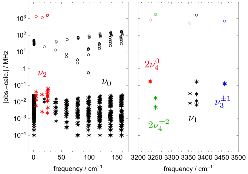
Figure 1: Absolute values of the discrepancies of the calculated transition frequencies of $\text{NH}_{3}$ to the experimental data for (left panel) the ground $\nu_{0}$ and $\nu_{2}$ vibrational states and (right panel) the $\nu_{1}$, $\nu_{3}^{\pm 1}$, $2\nu_{4}^{0}$, $2\nu_{4}^{\pm 2}$ bands. The errors in the rovibrational frequencies are plotted with circles while the relative errors of the quadrupole splittings are plotted with stars.

In Figure 1 we compare the predicted quadrupole hyperfine transition frequencies for $\text{NH}_{3}$ with the available experimental data. We have chosen the most recent and easily digitized experimental data sets, which contain rotational transitions in the ground vibrational Coudert and Roueff (2006) and $\nu_{2}$ Belov, Urban, and Winnewisser (1998) states, and rovibrational transitions from the ground to the $\nu_{1}$, $\nu_{3}^{\pm 1}$, $2\nu_{4}^{0}$, and $2\nu_{4}^{\pm 2}$ vibrational states Dietiker et al. (2015). An extended survey of the published experimental and theoretical data for the quadrupole hyperfine structure of ammonia can be found elsewhere Dietiker et al. (2015); Augustovičová, Soldán, and Špirko (2016). The absolute errors in the rovibrational frequencies, plotted with circles, are within the accuracy of the underlying PES Yurchenko et al. (2011). To estimate the accuracy of the predicted quadrupole splittings, we subtracted the respective error in the rovibrational frequency unperturbed from the quadrupole interaction effect for each transition. The resulting errors, plotted with stars in Figure 1, range from 0.1 to 25 kHz for the ground vibrational state and from 2.6 to 64 kHz for the $\nu_{2}$ state. These values correspond to the maximal relative errors in computed hyperfine splittings of 0.6 % and 1.4 % for the ground and $\nu_{2}$ states, respectively. For other fundamental and overtone bands, these errors are bigger, up to 160 kHz (3.9 %), however, the estimated uncertainty of the experimental data already accounts for $\pm 100$ (2.4 %) kHz Dietiker et al. (2015).

We believe that the accuracy of the quadrupole splittings can be significantly improved by employing a better level of the electronic structure theory in the calculations of the EFG surface. For example, the aug-cc-pVQZ basis set incompleteness error and the core electron correlation effects were shown to contribute up to 0.004 a.u. and 0.01 a.u., respectively, into the absolute values of the EFG tensor of the water molecule Olsen et al. (2002). By scaling these values with the nuclear quadrupole constant of the ¹⁴N atom, we estimate that the electronic structure errors in the quadrupole splittings of ammonia are as large as 50 kHz.

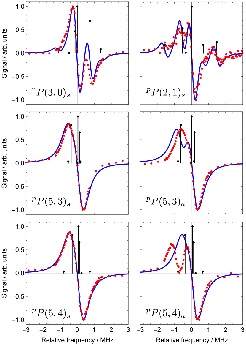
Figure 2: Comparison of the calculated (blue line) and observed Twagirayezu, Hall, and Sears (2016) (red dots) saturation dip line shapes for ${}^{\Delta K_{a}}\Delta J(J^{\prime\prime},K_{a}^{\prime\prime})_{\tau_{\rm inv}^{\prime\prime}}$ transitions of the $\nu_{1}+\nu_{3}$ band of NH₃ ($\tau_{\rm inv}^{\prime\prime}=s~{}{\rm or}~{}a$ denotes symmetric or anti-symmetric inversion parity of the ground vibrational state). Stems show contributing to the calculated line shape stick spectrum. The experimental and calculated intensities are normalized to the respective maximal values. The measured (calculated) zero-crossing wavenumbers, in $\text{cm}^{-1}$, are 6544.32154 (6544.49333) for ${}^{r}P(3,0)_{s}$, 6572.85349 (6572.87926) for ${}^{p}P(2,1)_{s}$, 6529.18969 (6530.047789) for ${}^{p}P(5,3)_{s}$, 6528.76857 (6528.51408) for ${}^{p}P(5,3)_{a}$, 6536.59280 (6537.31784) for ${}^{p}P(5,4)_{s}$, and 6537.68063 (6536.68512) for ${}^{p}P(5,4)_{a}$.

In Figure 2 we compare our results with sub-Doppler saturation-dip spectroscopic measurements for the $\nu_{1}+\nu_{3}$ band of $\text{NH}_{3}$ Twagirayezu, Hall, and Sears (2016). The saturation-dip lineshapes were calculated as the intensity-weighted sums of Lorentzian-lineshape derivatives Axner, Kluczynski, and Lindberg (2001) with a half-width-at-half-maximum (HWHM) width of the absorption profile of 290 kHz and the HWHM-amplitude of the experimentally applied frequency-modulation dither of 150 kHz Sears (2017). The ${}^{p}P(5,K_{a}^{\prime\prime})$ transitions were recorded with slightly larger HWHM Sears (2017) and we found a value of 500 kHz to best reproduce the measured lineshapes for these transitions. The computed profiles for ${}^{r}P(3,0)_{s}$, ${}^{p}P(2,1)_{s}$, ${}^{p}P(5,3)_{s}$, and ${}^{p}P(5,4)_{s}$ transitions show very good agreement with the measurement. For ${}^{p}P(5,3)_{a}$ and ${}^{p}P(5,4)_{a}$ transitions the calculated profiles do not match the experiment very well. In the experimental work Twagirayezu, Hall, and Sears (2016), the predicted double peak feature of the ${}^{p}P(5,3)_{a}$ was not observed while for the ${}^{p}P(5,4)_{a}$ it was attributed to perturbations. Based on the results of the present variational calculations the latter can not be confirmed. It should be noted, however, that the accuracy of the underlying PES is not sufficiently high in this energy region at 1.5 µm to unambiguously match the predicted rovibrational frequencies with the measured ones. Moreover, the PES employed here was obtained by a refinement of the ab initio surface to the high resolution spectroscopic data of NH₃. It is well known, that the PES refinement may cause appearance of the spurious intensity borrowing effects as well as dissipation of the true accidental resonances in various regions of the spectrum Yachmenev, Polyak, and Thiel (2013); Al-Refaie et al. (2015). Therefore, we refrain here from discussion of the possible alternative assignment of the ${}^{p}P(5,3)_{a}$ and ${}^{p}P(5,4)_{a}$ transitions. Calculations of a new, more accurate PES of NH₃ are currently performed and analyzed Coles, Yurchenko, and Tennyson (2017), which, once available, will be used to generate a more accurate quadrupole-hyperfine-resolved spectrum.

In conclusion, we have presented the first general-molecule variational implementation of nuclear-quadrupole hyperfine effects. Our approach is based on TROVE, which provides accurate spin-free rovibrational energy levels and wave functions used as a basis for the quadrupole-coupling problem. The initial results for ${}^{14}\text{NH}_{3}$ are in very good agreement with the available experimental data. The generated rovibrational line list for ${}^{14}\text{NH}_{3}$ with quadrupole-coupling components is available as part of the supplementary material Yac . We believe that computed hyperfine-resolved rovibrational spectrum of ammonia will be beneficial for the assignment of high resolution measurements in the near-infrared.

Calculations based on more accurate PES and the extension of the present approach to incorporate the hyperfine effects due to the spin-spin and spin-rotation couplings are currently performed in our group. Due to the general approach, predictions of similar quality will be possible for other small polyatomic molecules in order to guide future laboratory and astronomical observations with sub-Doppler resolution, including investigations of para-ortho transitions Miani and Tennyson (2004); Horke et al. (2014) or proton-to-electron-mass variations van Veldhoven et al. (2004); Cheng et al. (2016).

We gratefully acknowledge Trevor Sears for providing us with their original experimental data Twagirayezu, Hall, and Sears (2016). Besides DESY, this work has been supported by the excellence cluster “The Hamburg Center for Ultrafast Imaging—Structure, Dynamics and Control of Matter at the Atomic Scale” of the Deutsche Forschungsgemeinschaft (CUI, DFG-EXC1074).

References

- DeMille (2015) D. DeMille, “Diatomic molecules, a window onto fundamental physics,” Phys. Today 68, 34–40 (2015).
- Bethlem et al. (2008) H. L. Bethlem, M. Kajita, B. Sartakov, G. Meijer, and W. Ubachs, “Prospects for precision measurements on ammonia molecules in a fountain,” Eur. Phys. J. Special Topics 163, 55–69 (2008).
- Schnell and Küpper (2011) M. Schnell and J. Küpper, “Tailored molecular samples for precision spectroscopy experiments,” Faraday Disc. 150, 33–49 (2011).
- Bell and Softley (2009) M. T. Bell and T. P. Softley, “Ultracold molecules and ultracold chemistry,” Mol. Phys. 107, 99–132 (2009).
- van de Meerakker et al. (2012) S. Y. T. van de Meerakker, H. L. Bethlem, N. Vanhaecke, and G. Meijer, “Manipulation and control of molecular beams,” Chem. Rev. 112, 4828–4878 (2012).
- Naulin and Costes (2014) C. Naulin and M. Costes, “Experimental search for scattering resonances in near cold molecular collisions,” Int. Rev. Phys. Chem. 33, 427–446 (2014).
- Stuhl, Hummon, and Ye (2014) B. K. Stuhl, M. T. Hummon, and J. Ye, “Cold state-selected molecular collisions and reactions,” Annu. Rev. Phys. Chem. 65, 501–518 (2014).
- Baranov et al. (2012) M. A. Baranov, M. Dalmonte, G. Pupillo, and P. Zoller, “Condensed matter theory of dipolar quantum gases,” Chem. Rev. 112, 5012–5061 (2012).
- Ospelkaus et al. (2010) S. Ospelkaus, K.-K. Ni, G. Quéméner, B. Neyenhuis, D. Wang, M. H. G. de Miranda, J. L. Bohn, J. Ye, and D. S. Jin, “Controlling the hyperfine state of rovibronic ground-state polar molecules,” Phys. Rev. Lett. 104, 030402 (2010).
- Aldegunde, Ran, and Hutson (2009) J. Aldegunde, H. Ran, and J. M. Hutson, “Manipulating ultracold polar molecules with microwave radiation: The influence of hyperfine structure,” Phys. Rev. A 80, 043410 (2009).
- Moses et al. (2016) S. A. Moses, J. P. Covey, M. T. Miecnikowski, D. S. Jin, and J. Ye, “New frontiers for quantum gases of polar molecules,” Nat. Phys. 13, 13–20 (2016).
- Wei et al. (2011) Q. Wei, S. Kais, B. Friedrich, and D. Herschbach, “Entanglement of polar symmetric top molecules as candidate qubits,” J. Chem. Phys. 135, 154102 (2011).
- Jaouadi et al. (2013) A. Jaouadi, E. Barrez, Y. Justum, and M. Desouter-Lecomte, “Quantum gates in hyperfine levels of ultracold alkali dimers by revisiting constrained-phase optimal control design,” J. Chem. Phys. 139, 014310 (2013).
- van Veldhoven et al. (2004) J. van Veldhoven, J. Küpper, H. L. Bethlem, B. Sartakov, A. J. A. van Roij, and G. Meijer, “Decelerated molecular beams for high-resolution spectroscopy: The hyperfine structure of 15ND3,” Eur. Phys. J. D 31, 337–349 (2004).
- Flambaum and Kozlov (2007) V. V. Flambaum and M. G. Kozlov, “Limit on the cosmological variation of m(p)/m(e) from the inversion spectrum of ammonia,” Phys. Rev. Lett. 98, 240801 (2007).
- Owens et al. (2016) A. Owens, S. N. Yurchenko, W. Thiel, and V. Špirko, “Enhanced sensitivity to a possible variation of the proton-to-electron mass ratio in ammonia,” Phys. Rev. A 93, 052506 (2016).
- Cheng et al. (2016) C. Cheng, A. P. P. van der Poel, P. Jansen, M. Quintero-Pérez, T. E. Wall, W. Ubachs, and H. L. Bethlem, “Molecular fountain,” Phys. Rev. Lett. 117, 253201 (2016).
- Twagirayezu, Hall, and Sears (2016) S. Twagirayezu, G. E. Hall, and T. J. Sears, “Quadrupole splittings in the near-infrared spectrum of 14NH3,” J. Chem. Phys. 145, 144302 (2016).
- Hougen (1972) J. T. Hougen, “Reinterpretation of molecular beam hyperfine data for 14NH3 and 15NH3,” J. Chem. Phys. 57, 4207–4217 (1972).
- Gordy and Cook (1984) W. Gordy and R. L. Cook, Microwave Molecular Spectra, 3rd ed. (John Wiley & Sons, New York, NY, USA, 1984).
- Jensen et al. (1991) P. Jensen, I. Paidarová, J. Vojtík, and V. Špirko, “Theoretical calculations of the nuclear quadrupole coupling in the spectra of D, H2D+, and HD,” J. Mol. Spec. 150, 137–163 (1991).
- Jensen and Sauer (1997) P. Jensen and S. P. A. Sauer, “Theoretical calculations of the hyperfine structure in the spectra of H and its deuterated isotopomers,” Mol. Phys. 91, 319–332 (1997).
- Miani and Tennyson (2004) A. Miani and J. Tennyson, “Can ortho–para transitions for water be observed?” J. Chem. Phys. 120, 2732–2739 (2004).
- Lauvergnat and Nauts (2002) D. Lauvergnat and A. Nauts, “Exact numerical computation of a kinetic energy operator in curvilinear coordinates,” J. Chem. Phys. 116, 8560 (2002).
- Yurchenko, Thiel, and Jensen (2007) S. N. Yurchenko, W. Thiel, and P. Jensen, “Theoretical ROVibrational energies (TROVE): A robust numerical approach to the calculation of rovibrational energies for polyatomic molecules,” J. Mol. Spec. 245, 126–140 (2007).
- Mátyus et al. (2007) E. Mátyus, G. Czakó, B. T. Sutcliffe, and A. G. Császár, “Vibrational energy levels with arbitrary potentials using the Eckart-Watson Hamiltonians and the discrete variable representation,” J. Chem. Phys. 127, 084102 (2007).
- Mátyus, Czakó, and Császár (2009) E. Mátyus, G. Czakó, and A. G. Császár, “Toward black-box-type full- and reduced-dimensional variational (ro)vibrational computations,” J. Chem. Phys. 130, 134112 (2009).
- Wang and Carrington (2009) X.-G. Wang and T. Carrington, “A discrete variable representation method for studying the rovibrational quantum dynamics of molecules with more than three atoms,” J. Chem. Phys. 130, 094101 (2009).
- Avila and Carrington (2013) G. Avila and T. Carrington, “Solving the Schrödinger equation using smolyak interpolants,” J. Chem. Phys. 139, 134114 (2013).
- Fábri, Mátyus, and Császár (2011) C. Fábri, E. Mátyus, and A. G. Császár, “Rotating full- and reduced-dimensional quantum chemical models of molecules,” J. Chem. Phys. 134, 074105 (2011).
- Yachmenev and Yurchenko (2015) A. Yachmenev and S. N. Yurchenko, “Automatic differentiation method for numerical construction of the rotational-vibrational Hamiltonian as a power series in the curvilinear internal coordinates using the Eckart frame,” J. Chem. Phys. 143, 014105 (2015).
- Yurchenko, Yachmenev, and Ovsyannikov (2017) S. N. Yurchenko, A. Yachmenev, and R. I. Ovsyannikov, “Symmetry adapted ro-vibrational basis functions for variational nuclear motion calculations: TROVE approach,” J. Chem. Theory Comput. (2017), 10.1021/acs.jctc.7b00506, accepted.
- Tennyson et al. (2016) J. Tennyson, S. N. Yurchenko, A. F. Al-Refaie, E. J. Barton, K. L. Chubb, P. A. Coles, S. Diamantopoulou, M. N. Gorman, C. Hill, A. Z. Lam, L. Lodi, L. K. McKemmish, Y. Na, A. Owens, O. L. Polyansky, T. Rivlin, C. Sousa-Silva, D. S. Underwood, A. Yachmenev, and E. Zak, “The ExoMol database: Molecular line lists for exoplanet and other hot atmospheres,” J. Mol. Spec. 327, 73 – 94 (2016), new Visions of Spectroscopic Databases, Volume {II}.
- Yurchenko et al. (2011) S. N. Yurchenko, R. J. Barber, J. Tennyson, W. Thiel, and P. Jensen, “Towards efficient refinement of molecular potential energy surfaces: Ammonia as a case study,” J. Mol. Spec. 268, 123–129 (2011).
- Yurchenko et al. (2009) S. N. Yurchenko, R. J. Barber, A. Yachmenev, W. Thiel, P. Jensen, and J. Tennyson, “A variationally computed K line list for NH3,” J. Phys. Chem. A 113, 11845–11855 (2009).
- Derzi et al. (2015) A. R. A. Derzi, T. Furtenbacher, J. Tennyson, S. N. Yurchenko, and A. G. Császár, “MARVEL analysis of the measured high-resolution spectra of 14NH3,” J. Quant. Spectrosc. Radiat. Transfer 161, 117–130 (2015).
- Coudert and Roueff (2006) L. H. Coudert and E. Roueff, “Linelists for NH3, NH2D, ND2H, and ND3 with quadrupole coupling hyperfine components,” Astron. Astrophys. 449, 855–859 (2006).
- Belov, Urban, and Winnewisser (1998) S. Belov, Š. Urban, and G. Winnewisser, “Hyperfine structure of rotation-inversion levels in the excited 2 state of ammonia,” J. Mol. Spec. 189, 1–7 (1998).
- Dietiker et al. (2015) P. Dietiker, E. Miloglyadov, M. Quack, A. Schneider, and G. Seyfang, “Infrared laser induced population transfer and parity selection in 14NH3: A proof of principle experiment towards detecting parity violation in chiral molecules,” J. Chem. Phys. 143, 244305 (2015).
- Cook and de Lucia (1971) R. L. Cook and F. C. de Lucia, Am. J. Phys. 39, 1433–1454 (1971).
- (41) All supplementary data are available online at https://doi.org/10.5281/zenodo.855339.
- Yachmenev and Owens (2017) A. Yachmenev and A. Owens, “A general TROVE-based variational approach for rovibrational molecular dynamics in external electric fields,” J. Chem. Phys. (2017), in preparation.
- Yurchenko, Barber, and Tennyson (2011) S. N. Yurchenko, R. J. Barber, and J. Tennyson, “A variationally computed line list for hot NH3,” Mon. Not. Royal Astron. Soc. 413, 1828–1834 (2011).
- Dunning (1989) T. H. Dunning, J. Chem. Phys. 90, 1007 (1989).
- Kendall, Jr., and Harrison (1992) R. A. Kendall, T. H. D. Jr., and R. J. Harrison, “Electron affinities of the first-row atoms revisited. Systematic basis sets and wave functions,” J. Chem. Phys. 96, 6796–6806 (1992).
- Scuseria (1991) G. E. Scuseria, “Analytic evaluation of energy gradients for the singles and doubles coupled cluster method including perturbative triple excitations: Theory and applications to FOOF and Cr2,” J. Chem. Phys. 94, 442–447 (1991).
- (47) CFOUR, Coupled-Cluster techniques for Computational Chemistry, a quantum chemical program package written by J. F. Stanton, J. Gauss, M. E. Harding, and P. G. Szalay with contributions from A. A. Auer, R. J. Bartlett, U. Benedikt, C. Berger, D. E. Bernholdt, Y. J. Bomble, L. Cheng, O. Christiansen, M. Heckert, O. Heun, C. Huber, T.-C. Jagau, D. Jonsson, J. Jusélius, K. Klein, W. J. Lauderdale, D. A. Matthews, T. Metzroth, L. A. Mück, D. P. O’Neill, D. R. Price, E. Prochnow, C. Puzzarini, K. Ruud, F. Schiffmann, W. Schwalbach, S. Stopkowicz, A. Tajti, J. Vázquez, F. Wang, J. D. Watts, and the integral packages MOLECULE (J. Almlöf and P. R. Taylor), PROPS (P. R. Taylor), ABACUS (T. Helgaker, H. J. Aa. Jensen, P. Jørgensen, and J. Olsen), and ECP routines by A. V. Mitin and C. van Wüllen. For the current version, see http://www.cfour.de.
- Pyykkö (2008) P. Pyykkö, “Year-2008 nuclear quadrupole moments,” Mol. Phys. 106, 1965–1974 (2008).
- Augustovičová, Soldán, and Špirko (2016) L. Augustovičová, P. Soldán, and V. Špirko, “Effective Hyperfine-Structure Functions of Ammonia,” Astrophys. J. 824, 147 (2016).
- Note (1) We note that we found some inconsistencies in the experimental results reported in Table VIII of reference \rev@citealpnumDietiker:JCP143:244305, which we have corrected in our analysis.
- Olsen et al. (2002) L. Olsen, O. Christiansen, L. Hemmingsen, S. P. A. Sauer, and K. V. Mikkelsen, “Electric field gradients of water: A systematic investigation of basis set, electron correlation, and rovibrational effects,” J. Chem. Phys. 116, 1424–1434 (2002).
- Axner, Kluczynski, and Lindberg (2001) O. Axner, P. Kluczynski, and Å. M. Lindberg, “A general non-complex analytical expression for the th Fourier component of a wavelength-modulated Lorentzian lineshape function,” J. Quant. Spectrosc. Radiat. Transfer 68, 299–317 (2001).
- Sears (2017) T. J. Sears, private communication (2017).
- Yachmenev, Polyak, and Thiel (2013) A. Yachmenev, I. Polyak, and W. Thiel, “Theoretical rotation-vibration spectrum of thioformaldehyde,” J. Chem. Phys. 139, 204308 (2013).
- Al-Refaie et al. (2015) A. F. Al-Refaie, A. Yachmenev, J. Tennyson, and S. N. Yurchenko, “ExoMol line lists - VIII. a variationally computed line list for hot formaldehyde,” Mon. Not. Royal Astron. Soc. 448, 1704–1714 (2015).
- Coles, Yurchenko, and Tennyson (2017) P. Coles, S. N. Yurchenko, and J. T. Tennyson, (2017), in preparation.
- Horke et al. (2014) D. A. Horke, Y.-P. Chang, K. Długołęcki, and J. Küpper, “Separating para and ortho water,” Angew. Chem. Int. Ed. 53, 11965–11968 (2014), arXiv:1407.2056 [physics] .