Mean field theory of the swap Monte Carlo algorithm

Abstract

The swap Monte Carlo algorithm combines the translational motion with the exchange of particle species, and is unprecedentedly efficient for some models of glass former. In order to clarify the physics underlying this acceleration, we study the problem within the mean field replica liquid theory. We extend the Gaussian ansatz so as to take into account the exchange of particles of different species, and we calculate analytically the dynamical glass transition points corresponding to the swap and standard Monte Carlo algorithms. We show that the system evolved with the standard Monte Carlo algorithm exhibits the dynamical transition before that of the swap Monte Carlo algorithm. We also test the result by performing computer simulations of a binary mixture of the Mari-Kurchan model, both with standard and swap Monte Carlo. This scenario provides a possible explanation for the efficiency of the swap Monte Carlo algorithm. Finally, we discuss how the thermodynamic theory of the glass transition should be modified based on our results.

I Introduction

In many materials, with decreasing the temperature or increasing the density, the supercooled liquids dynamics shows dramatic slowing down and eventually gets frozen without developing any crystalline order. This is the so-called glass transition Debenedetti and Stillinger (2001); Cavagna (2009); Gotze (2009); Berthier and Biroli (2011); Biroli and Garrahan (2013).

One of the promising theory to explain the glass transition is the so-called random first order phase transition theory (RFOT) Kirkpatrick and Wolynes (1987); Kirkpatrick et al. (1989); Bouchaud and Biroli (2004); Lubchenko and Wolynes (2007); Kirkpatrick and Thirumalai (2015), which attributes the slow dynamics to the emergence of a very large number of long-lived metastable states. It has been shown that the RFOT scenario holds exactly in the high dimensional limit Parisi and Zamponi (2010); Charbonneau et al. (2017). In finite dimensions, there are several systematic approximation schemes that allow one to calculate the quantitative values of the thermodynamic quantities Mézard and Parisi (1999a, b); Parisi and Zamponi (2005, 2010); Jacquin et al. (2011); Berthier et al. (2011); Mangeat and Zamponi (2016). The RFOT theory predicts the existence of two important transition densities (temperatures). The first is the dynamical glass transition point, $\varphi_{d}$ [see Eq. (5) for a precise definition of packing fraction $\varphi$ in our model], at which exponentially many metastable glassy states arise in the free energy landscape. At the mean-field level, or equivalently, at the high dimension limit, the lifetime of the metastable state is infinite and the relaxation time diverges. The divergent behavior of the relaxation time upon approaching $\varphi_{d}$ from the liquid side is well described by the mode coupling theory (MCT) Bengtzelius et al. (1984); Gotze (2009), which was first independently derived by kinetic theory and later integrated in the RFOT scenario Kirkpatrick and Wolynes (1987); Maimbourg et al. (2016). In finite dimensions, contrary to the high dimensional limit, the dynamical transition is avoided and the lifetime of the metastable states is finite even above $\varphi_{d}$. Above $\varphi_{d}$, the relaxation is controlled by the configurational entropy, which is the logarithm of the number of metastable states Adam and Gibbs (1965); Kirkpatrick et al. (1989); Bouchaud and Biroli (2004). With increasing the density, the configurational entropy decreases and eventually vanishes at the thermodynamic glass transition point, the so-called Kauzmann transition point, $\varphi_{K}$ Kauzmann (1948). Above $\varphi_{K}$, the system is permanently trapped in the lowest free energy state, called the ideal glass state. It is quite challenging to reach the genuine thermodynamic glass transition point, if any, because the relaxation time of the supercooled liquid increases very rapidly above $\varphi_{d}$ and the system easily goes out of equilibrium while still being far from $\varphi_{K}$. Still, several indirect evidences that support the existence of the thermodynamic glass transition have been reported, including a growing static correlation length Bouchaud and Biroli (2004); Biroli et al. ; Berthier and Kob (2012) and an ideal glass transition in randomly pinned systems Cammarota and Biroli (2012, 2013); Karmakar and Parisi (2013); Kob and Berthier (2013); Ozawa et al. (2015).

Even if a thermodynamic glass transition exists, it is still unclear whether or not such a transition would be the main ingredient inducing slow dynamics in real supercooled liquids. Indeed, a totally different scenario to explain the slow dynamics has been proposed. The so-called dynamical facilitation theory (DFT) claims that kinetic constraints play an essential role in the slow dynamics of supercooled liquids Ritort and Sollich (2003); Chandler and Garrahan (2010); Biroli and Garrahan (2013). Under this assumptions, the theory describes well the qualitative behavior of the relaxation time in finite dimensions Biroli and Garrahan (2013); Keys et al. (2011); Isobe et al. (2016). Furthermore, on the Bethe lattice, the Fredrickson-Andersen (FA) model Fredrickson and Andersen (1984), which is a typical model in the DFT class, exhibits very similar behavior to the MCT Sellitto et al. (2005, 2010); Ikeda and Miyazaki (2015); Sellitto (2015); De Candia et al. (2016); Ikeda et al. (2017). Also, in finite dimensions, a Kac version of the FA model describes well the avoided dynamical transition Berthier et al. (2012). These successes of the DFT suggest that dynamic rules are indeed important.

To clarify the effects of the dynamic rules on the slow dynamics of supercooled liquids, it is helpful to observe the dynamic rule dependence. If the slow dynamics is originated solely by a thermodynamic glass transition, the dynamical behavior of supercooled liquids should depend only weakly on the details of the rules governing the dynamics Wyart and Cates (2017). This assumption is however inconsistent with recent results obtained by computer simulations using the swap Monte Carlo algorithm (swap MC) Gazzillo and Pastore (1989); Grigera and Parisi (2001); Cavagna et al. (2012); Gutiérrez et al. (2015); Berthier et al. (2016); Ninarello et al. (2017); Berthier et al. (2017). The swap MC combines the standard Monte Carlo algorithm with the exchange of particles species. The computer simulations of some polydisperse systems demonstrate that the swap MC can equilibrate the system about 10 orders of magnitude faster than the standard MC Berthier et al. (2016); Ninarello et al. (2017); Berthier et al. (2017). Clearly, the standard RFOT scenario fails to explain this result, because it totally neglects the details of the systems dynamics. It is thus desirable to reformulate the RFOT scenario so as to take into account the effects of the dynamic rule.

In this work, we perform a first step in this direction, by investigating the binary Mari-Kurchan (MK) model Mari and Kurchan (2011); Charbonneau et al. (2014), which is a mean-field model belonging to the RFOT class, with the swap and standard MC algorithms. We separately calculate the dynamical glass transition point with the swap MC, $\varphi_{d}^{\rm swap}$, and with the standard MC, $\varphi_{d}^{\rm mc}$, and we show that $\varphi_{d}^{\rm mc}<\varphi_{d}^{\rm swap}$. We also perform computer simulations of the binary MK model and compare with the analytical result, showing in particular that between $\varphi_{d}^{\rm mc}$ and $\varphi_{d}^{\rm swap}$, the swap MC is more efficient than the standard MC. Finally, we discuss the thermodynamic glass transition and the relaxation dynamics above the dynamical transition point of more realistic glass forming systems.

The organization of the paper is as follows. In Sec. II, we roughly sketch the main idea of our theory. In Sec. III, we introduce the model. In Sec. IV, we derive the analytical expression of the free energy. In Sec. V, we calculate the order parameters and phase diagram from the free energy. In Sec. VI, we report the computer simulation and compare with the theoretical results. In Sec. VII, we discuss the configurational entropy, the thermodynamic glass transition point, and the activated dynamics. In Sec. VIII, we summarize the results and conclude the work.

II Sketch of the framework

Before going into the details of the theory and the model, here we give a qualitative explanation of our theory. Within the RFOT scenario, the slow dynamics is attributed to the emergence of long-lived glassy metastable states. The dynamics within one of these states is assumed to be arrested on the experimental time scale. This dynamical arrest manifests itself in the two-time correlation functions, such as the mean square displacement or the intermediate scattering functions. In particular, if $\bm{x}_{i}(t)$ is the position of particle $i$ at time $t$, the mean square displacement (MSD) is defined as

$${\rm MSD}(t) \equiv\frac{1}{N}\sum_{i=1}^{N}\left\langle\left(\bm{x}_{i}(t)-\bm{x}_{i}(0)\right)^{2}\right\rangle.$$ (1)

In the liquid phase, the long-time limit of the MSD is diffusive, ${\rm MSD}(t)\sim 2dDt$ for $t\to\infty$, where $D$ is the diffusion constant. In the glass phase, instead (at least in the mean field limit), the long time limit of the MSD is a constant, expressing the fact that particles are caged by their neighbors and cannot diffuse, so they remain close to their initial position at all times. One can think of the swap algorithm as a dynamics in which a given particle does not have a definite type and it can exchange its type with other particles during the dynamical evolution Ninarello et al. (2017). The question is therefore whether such an exchange process can facilitate the dynamical relaxation, leading to an increased efficiency of the swap algorithm.

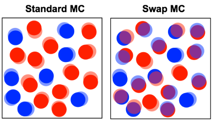
Figure 1: Schematic representation of the dynamics in a glass state, and its translation into the replica framework. Here, the circles describe the position of particles, while the different colors describe the different species. The transparent and non-transparent symbols correspond to the initial configuration (encoded by replica 1) and the long-time configuration (encoded by replica 2), respectively. In the standard MC ansatz, we assume that in the glass phase particles keep their identity at all times (i.e. exchanges are forbidden), so that in different replicas, the same particle must of the same type. In the swap MC phase, we assume that in the glass phase particles can change type during time, so that in different replicas, the same particle can have different types.

If the dynamical arrest is related to the emergence of metastable states, it can be captured by a purely thermodynamic calculation: this is indeed the essence of the RFOT scenario. Such a calculation can be performed via the so-called replica liquid theory (RLT) Monasson (1995), in which long-time correlations in the dynamics are translated in correlations between different copies of the original system (replicas); see Refs. Mézard and Parisi (1999a, b); Parisi and Zamponi (2010) for details. We thus introduce replicas, which can be thought as configurations of the same glass separated by an extremely long time evolution. In the liquid phase, as the system diffuses, the different replicas are uncorrelated. Above the dynamical glass transition point, $\varphi_{d}$, many metastable states arise. In the metastable states, because diffusion is arrested, the same particles of different replicas remain close together, and can be thus thought as “molecules” Mézard and Parisi (1999a, b); Parisi and Zamponi (2010).

Our central assumption is that different kind of molecules describe different dynamical rules, as illustrated in Fig. 1.

• In the case of the standard MC without particle swap, we assume that particles of different species can not be exchanged in a glassy metastable state, or more precisely, that the typical time scale to exchange particles of different species is much longer than the lifetime of the metastable state itself. Hence, a particle keeps its identity at all times, and as a consequence, the replica molecules must consist of particles of the same species, see the left cartoon of Fig. 1.

• This assumption is inappropriate in the case of the swap MC, because particles of different species can be exchanged much more easily than in the standard MC. In this case, we thus assume that in the glass phase, particles can still change their identity over time, and the replica molecules can thus consist of particles of different species, see the right cartoon of Fig. 1. This kind of ansatz was first proposed by Coluzzi et al. Coluzzi et al. (1999) and later explicitly implemented by Ikeda et al. Ikeda et al. (2016).

The assumptions that the long-time correlations are different in the standard and swap MC dynamics, and that they can be encoded in different replica ansatzes, are the crucial working hypothesis behind our analysis; we believe that it should hold at least in the mean field limit. In Sec. IV, we discuss the details of the two ansatzes and calculate $\varphi_{d}$ of the binary Mari-Kurchan model (MK model). In Sec. VI, we report a comparison of the theory with computer simulations of the same system, which provides strong support for the validity of our hypothesis in this system.

III Model

In this section, we introduce the model. We consider a system consisting of an equal number of large and small particles. The particles interact with the following potential:

$$V_{N} =\sum_{i<j}v_{\mu_{i}\mu_{j}}(\bm{x}_{i}-\bm{x}_{j}+\bm{\Lambda}_{ij}),$$ (2)

where

$$v_{\mu_{i}\mu_{j}}(\bm{x}_{i}-\bm{x}_{j}+\bm{\Lambda}_{ij}) =\begin{cases}\infty&\text{if }\left|\bm{x}_{i}-\bm{x}_{j}+\bm{\Lambda}_{ij}\right|\leq\sigma_{\mu_{i}\mu_{j}}\\ 0&\text{if }\left|\bm{x}_{i}-\bm{x}_{j}+\bm{\Lambda}_{ij}\right|>\sigma_{\mu_{i}\mu_{j}}\\ \end{cases}.$$ (3)

Here, $\bm{x}_{i},\bm{x}_{j}\in\mathbb{R}^{d}$ denote the particle positions and $\mu_{i},\mu_{j}\in\{L,\ S\}$ denote the particle species. $\sigma_{LL}$, $\sigma_{SS}$ are the diameters of large and small particles, respectively. We assume that the potential is additive, $\sigma_{LS}=\sigma_{SL}=(\sigma_{LL}+\sigma_{SS})/2$. $\bm{\Lambda}_{ij}$ is a quenched randomness and for each pair of $i<j$, $\bm{\Lambda}_{ij}$ is generated independently from the probability distribution function,

$$P(\bm{\Lambda}_{ij})=\frac{1}{V},$$ (4)

where $V$ is the volume of the system. The total number of particles is $N=N_{L}+N_{S}$, with particle concentrations $x_{\mu}=N_{\mu}/N$. The number density is $\rho=N/V$, and the packing fraction is given, in the case $d=3$ which will be our focus in the following, by

$$\varphi=\frac{\pi}{6}\rho[x_{L}\sigma_{LL}^{3}+x_{S}\sigma_{SS}^{3}]\ .$$ (5)

We also impose $\bm{\Lambda}_{ij}=-\bm{\Lambda}_{ji}$ so that the shifted distance between the $i$-th and $j$-th particles is to be symmetric,

$$\left|\bm{x}_{i}-\bm{x}_{j}+\bm{\Lambda}_{ij}\right|=\left|\bm{x}_{j}-\bm{x}_{i}+\bm{\Lambda}_{ji}\right|.$$ (6)

Because of the quenched randomness, $\bm{\Lambda}_{ij}$, particles interact with other randomly chosen particles instead of their nearest neighbor particles. The model is similar to models defined on random interaction graphs, and one can obtain the analytical expression of the free energy through mean field techniques Mari and Kurchan (2011).

IV Free energy calculation

In this section, we derive the analytical expression of the free energy. In case of the swap MC, one should take into account the exchange of the particle species as well as the translational motion of the particle position. The partition function can be written as

$$Z[\{\bm{\Lambda}_{ij}\}] =\prod_{i=1}^{N}\sum_{\mu_{i}}\int d\bm{x}_{i}e^{-\beta\sum_{i<j}v_{\mu_{i}\mu_{j}}(\bm{x}_{i}-\bm{x}_{j}+\bm{\Lambda}_{ij})},$$ (7)

where $N$ is the number of particles and $\beta$ is the inverse temperature. Note that the Gibbs factor $N!$ does not appear, because all particles are distinguishable due to the quenched randomness Mari and Kurchan (2011). Using the self-averaging property, the free energy can be calculated as

$$-\beta F\equiv\log Z[\{\bm{\Lambda}_{ij}\}]\approx\overline{\log Z[\{\bm{\Lambda}_{ij}\}]},$$ (8)

where the overline denotes averaging over $\bm{\Lambda}_{ij}$. We analyze the free energy using the replica method Mézard et al. (1987); Nishimori (2001). Because of the quenched disorder, the treatment might look different from the usual replica liquid theory Parisi and Zamponi (2010). However, as we will see below, the two methods are identical. To perform the disordered overage, we rewrite Eq. (8) as

$$-\beta F =\lim_{n\to 0}\frac{\log\overline{Z[\{\bm{\Lambda}_{ij}\}]^{n}}}{n}.$$ (9)

We shall use the one-step replica symmetric breaking ansatz (1RSB); we divide $n$ replicas into $n/m$ subgroups and assume that only the $m$ replicas in the same group are correlated Mézard et al. (1987); Nishimori (2001). The 1RSB structure, coupled to the fact that replicas in different blocks are completely uncorrelated (this property does not hold for all models), allows to factorize the partition function as $\overline{Z^{n}}=(\overline{Z^{m}})^{\frac{n}{m}}$. Substituting this expression into Eq. (9), one obtains

$$-\beta F =\frac{\log\overline{Z^{m}}}{m},$$ (10)

where

$$\overline{Z^{m}} =\prod_{i<j}\int d\bm{\Lambda}_{ij}P(\bm{\Lambda}_{ij})\left(\prod_{a=1}^{m}\prod_{i=1}^{N}\sum_{\mu_{i}^{a}}\int d\bm{x}_{i}^{a}\right)$$

$$\times\exp\left[-\beta\sum_{a=1}^{m}\sum_{i<j}v_{\mu_{i}^{a}\mu_{j}^{a}}(\bm{x}_{i}^{a}-\bm{x}_{j}^{a}+\bm{\Lambda}_{ij})\right].$$ (11)

Note that except for the factor $m^{-1}$, the free energy Eq. (10) is the same of the one considered in the standard replica liquid theory Parisi and Zamponi (2010). Thus, we can use the standard RLT of usual supercooled liquids without the quenched disorder. The partition function Eq. (11) can be analyzed using the saddle point method, see Ref. Mari and Kurchan (2011) for the details. After some straightforward calculations, we obtain

$$\mathcal{S}_{m}\equiv\frac{\log\overline{Z^{m}}}{N} =\log N-\frac{1}{N}\sum_{\overline{\mu}}\int d\overline{\bm{x}}\rho_{\overline{\mu}}(\overline{\bm{x}})\log\rho_{\overline{\mu}}(\overline{\bm{x}})$$

$$+\frac{1}{2N}\sum_{\overline{\mu},\overline{\nu}}\int d\overline{\bm{x}}d\overline{\bm{y}}\rho_{\overline{\mu}}(\overline{\bm{x}})\rho_{\overline{\nu}}(\overline{\bm{y}})f_{\overline{\mu},\overline{\nu}}(\overline{\bm{x}}-\overline{\bm{y}}),$$ (12)

where we have used the shorthand notations $\overline{\bm{x}}=\{\bm{x}^{1},\bm{x}^{2},\cdots,\bm{x}^{m}\}$ and $\overline{\mu}=\{\mu^{1},\mu^{2},\cdots,\mu^{m}\}$. We have also introduced the density distribution function,

$$\rho_{\overline{\mu}}(\overline{\bm{x}}) =\sum_{i=1}^{N}\left\langle\prod_{a=1}^{m}\delta(\bm{x}^{a}-\bm{x}_{i}^{a})\delta(\mu^{a},\mu_{i}^{a})\right\rangle,$$ (13)

and the replicated Mayer function,

$$f_{\overline{\mu}\overline{\nu}}(\overline{\bm{x}}-\overline{\bm{y}}) =\prod_{a=1}^{m}e^{-\beta v_{\mu^{a}\nu^{a}}(\bm{x}^{a}-\bm{y}^{a})}-1.$$ (14)

The full optimization of the free energy Eq. (12) for a completely general form of $\rho$ is a very difficult task. In order to simplify the calculations, below we approximate $\rho$ by assuming that it has a Gaussian form.

IV.1 Ansatz for the swap Monte Carlo algorithm

Here, we construct an ansatz for the swap MC. We simply assume that the distribution function can be factorized as

$$\rho_{\overline{\mu}}(\overline{\bm{x}})=\rho(\overline{\bm{x}})g(\overline{\mu}).$$ (15)

In principle, one can avoid this assumption and consider a more general ansatz, but the calculation becomes more involved as shown in Appendix. For the distribution function of the positions, we assume a Gaussian form Mézard and Parisi (1999a); Parisi and Zamponi (2010)

$$\rho(\overline{\bm{x}}) =\rho\int d\bm{X}\prod_{a=1}^{m}\gamma_{A}(\bm{x}^{a}-\bm{X}),$$ (16)

where $\gamma_{A}(\bm{x})=e^{-\left|\bm{x}\right|^{2}/2A}/(2\pi A)^{d/2}$. This is the same of that used for the one-component MK model Mari and Kurchan (2011); Parisi and Zamponi (2010), and we stress that this ansatz has no particular physical meaning, it is chosen only to make the calculation simpler. The cage size $A$ corresponds to the order parameter of the particle position. $A\to\infty$ corresponds to the liquid state, while a finite value of $A$ corresponds to the glass state. For $g(\overline{\mu})$, we assume the same form of the distribution function of the mean-field spin glasses Mézard et al. (1987); Hajime Yoshino :

$$g(\overline{\mu}) =C_{m}^{-1}e^{H\sum_{a}\sigma(\mu^{a})+\frac{\Delta^{2}}{2}\sum_{ab}\sigma(\mu^{a})\sigma(\mu^{b})}$$

$$=C_{m}^{-1}\int_{-\infty}^{\infty}Du\prod_{a=1}^{m}e^{(H+u)\sigma(\mu^{a})},$$ (17)

where $\sigma(L)=+1$, $\sigma(S)=-1$ (i.e. large particles are associated to up spins, small particles to down spins), and $Du=du\times e^{-u^{2}/2\Delta^{2}}/\sqrt{2\pi\Delta^{2}}$. $C_{m}$ is determined from the normalization condition, $\sum_{\overline{\mu}}g(\overline{\mu})=1$. $H$ fixes the numbers of large and small particles by

$$N_{\mu} =N\sum_{\overline{\mu}}g(\overline{\mu})\delta(\mu^{a},\mu),$$ (18)

where $N_{L}$ ($N_{S}$) is the number of large (small) particles. In particular for the equimolar system, $N_{L}=N_{S}$, which we shall investigate below, one can show that $H=0$. The correlation function of the particles species can be calculated as a function of $m$ and $\Delta$:

$$q_{m}(\Delta) \equiv\left\langle\sigma(\mu^{1})\sigma(\mu^{2})\right\rangle=\frac{\int Du\tanh(u)^{2}\cosh(u)^{m}}{\int Du\cosh(u)^{m}}\ .$$ (19)

In equilibrium, the order parameter of the glass transition is calculated by setting $m=1$ Parisi and Zamponi (2010). The function $q(\Delta)=q_{1}(\Delta)$ monotonically increases with $\Delta$ from zero to unity as shown in Fig. 2.

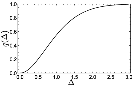
Figure 2: $\Delta$ dependence of $q(\Delta)$

$q$ (or $\Delta$) plays the role of the order parameter of the particle species. $q=0$ (or $\Delta=0$) corresponds to molecules made of completely uncorrelated particle types, and a finite value of $q$ (or $\Delta$) corresponds to molecules made of predominantly similar particles (i.e. finite correlation between particle types). The case $q=1$ (or $\Delta=\infty$) corresponds to fully identical particle types, as in the left panel of Fig. 1.

Substituting the above ansatz into the free energy, Eq. (12), we obtain

$$\mathcal{S}_{m} =\log N+\mathcal{S}_{id}^{x}+\mathcal{S}_{id}^{\sigma}+\mathcal{S}_{int},$$

$$\mathcal{S}_{id}^{x} =-\log\rho-\frac{d}{2}(1-m)\log(2\pi A)+\frac{d}{2}\log m-\frac{d}{2}(1-m),$$

$$\mathcal{S}_{id}^{\sigma} =\log C_{m}-\frac{\Delta^{2}}{2}\left(m+m(m-1)q_{m}(\Delta)\right),$$

$$\mathcal{S}_{int} =\frac{\rho}{2}\int d\bm{r}\left[\frac{1}{C_{m}^{2}}\int DuDvQ(\bm{r},u,v)^{m}-1\right],$$

where

$$C_{m} =\int Du\left[2\cosh(u)\right]^{m}$$ (21)

and

$$Q(\bm{r},u,v) =\sum_{\mu\nu}e^{u\sigma(\mu)+v\sigma(\nu)}\int d\bm{r}^{\prime}\gamma_{2A}(\bm{r}+\bm{r}^{\prime})e^{-\beta v_{\mu\nu}(\bm{r}^{\prime})}.$$ (22)

The order parameters, $A$ and $\Delta$, are determined by the saddle point conditions, $\partial_{A}\mathcal{S}_{m}=0$ and $\partial_{\Delta}\mathcal{S}_{m}=0$. In particular, we focus on the limit of $m\to 1$, which corresponds to the equilibrium glass transition Parisi and Zamponi (2010). In this limit, we obtain the following self-consistent equations:

$$A =\frac{1}{\rho}M_{A}(A,\Delta),$$

$$\Delta =M_{\Delta}(A,\Delta),$$

$$M_{A} =\left[-\frac{e^{-\Delta^{2}}}{4d}\int d\bm{r}\int DuDv\frac{\partial Q}{\partial A}\left[\log Q-f\right]\right]^{-1},$$

$$M_{\Delta} =-\frac{1}{1+q}\Bigg{[}-\frac{f^{\prime}}{2}+\frac{\Delta^{2}}{2}q^{\prime}$$

$$+\frac{\rho\Delta e^{-\Delta^{2}}}{4}\int d\bm{r}DuDvQ\left(\log Q-f\right)$$

$$-\frac{\rho e^{-\Delta^{2}}}{8}\int d\bm{r}Du^{\prime}DvQ\left(\log Q-f\right)$$

$$-\frac{\rho e^{-\Delta^{2}}}{8}\int d\bm{r}DuDv^{\prime}Q\left(\log Q-f\right)$$

$$+\frac{\rho e^{-\Delta^{2}}}{8}\int d\bm{r}DuDvQf^{\prime}\Bigg{]},$$ (23)

where we used the shorthand notation $F^{\prime}=\partial_{\Delta}F$ and introduced an auxiliary function;

$$f(\Delta) =e^{-\Delta^{2}/2}\int Du\,2\cosh(u)\log\left[2\cosh(u)\right].$$ (24)

IV.2 Ansatz for the standard Monte Carlo algorithm

In case of the standard MC without particle swap, we assume that particles of different species can not be exchanged. All $m$ replicas should have the same species, namely,

$$g(\overline{\mu}) =\sum_{\mu}x_{\mu}\prod_{a=1}^{m}\delta_{\mu^{a},\mu},$$ (25)

where $x_{\mu}=N_{\mu}/N$ is the number fraction of the $\mu$-species. This corresponds to the previous ansatz for $\Delta=\infty$. For $\rho(\overline{\bm{x}})$, we use the same Gaussian ansatz of the swap MC, Eq. (16). Substituting the ansatz into the free energy, Eq. (12), we obtain

$$\mathcal{S}_{m} =\log N+\mathcal{S}_{id}+\mathcal{S}_{int},$$

$$\mathcal{S}_{id} =\log 2-\log\rho-\frac{d}{2}(1-m)\log(2\pi A)$$ (26)

$$+\frac{d}{2}\log m-\frac{d}{2}(1-m),$$

$$\mathcal{S}_{int} =\frac{\rho}{2}\sum_{\mu\nu}x_{\mu}x_{\nu}\int d\bm{r}\left[Q_{\mu\nu}(\bm{r})^{m}-1\right],$$ (27)

where

$$Q_{\mu\nu}(\bm{r}) =\int d\bm{r}^{\prime}\gamma_{2A}(\bm{r}+\bm{r}^{\prime})e^{-\beta v_{\mu\nu}(\bm{r}^{\prime})}.$$ (28)

From the saddle point condition $\partial_{A}\mathcal{S}_{m}=0$, we can calculate the value of $A$. In the $m\to 1$ limit, we obtain

$$A =\frac{1}{\rho}M(A),$$ (29)

where

$$M(A) =\left[\frac{1}{d}\sum_{\mu\nu}x_{\mu}x_{\nu}\int d\bm{r}Q_{\mu\nu}\log Q_{\mu\nu}\right]^{-1}.$$ (30)

IV.3 Numerical solution of the equations

The self-consistent equations, Eqs. (23) and Eq. (29), can be solved iteratively. The dynamical glass transition point $\rho_{d}$ is defined as the density at which nontrivial solutions of the order parameters appear Parisi and Zamponi (2010). Near $\rho_{d}$ however, the iterative method becomes inefficient and it takes a long time to find the transition point in this way. An efficient way is to calculate the dynamical transition point from

$$\rho_{d}^{\rm swap} =\min_{A}\left[\frac{M_{A}(A,\Delta(A))}{A}\right],$$

$$\rho_{d}^{\rm mc} =\min_{A}\left[\frac{M(A)}{A}\right],$$ (31)

where $\Delta(A)$ is obtained by solving iteratively $\Delta=M_{\Delta}(A,\Delta)$.

V Order parameters and phase diagram

In this section, we discuss the density dependence of the order parameters and the phase diagram obtained by solving the self-consistent equations derived in Sec. IV.

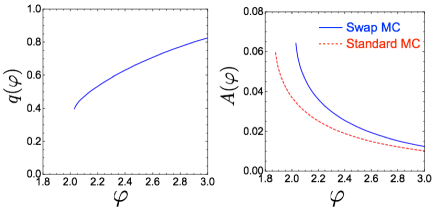
Figure 3: $\varphi$ dependence of the order parameters at $\sigma_{LL}/\sigma_{SS}=1.4$ and $d=3$. The blue solid lines denote the result of the swap MC (with order parameters $q$ and $A$), while the red dashed line denotes the result of the standard MC (with a single order parameter $A$).

We first discuss the behavior of the swap MC. We solve Eqs. (23) and calculate the order parameters of the swap MC, $q(\varphi)$ and $A(\varphi)$. The result at $\sigma_{LL}/\sigma_{SS}=1.4$ and $d=3$ is shown in Fig. 3 with the blue solid lines. For sufficiently small $\varphi$, $A=\infty$ and $\Delta=0$ indicating that there is no correlation between replicas and the system is in the liquid phase. As $\varphi$ is increased, $q(\varphi)$ jumps from zero to a finite value at the dynamical transition point, $\varphi_{d}^{\rm swap}\approx 2.02$. Simultaneously, $A(\varphi)$ drops from infinity to a finite value. This means that, even within the swap MC ansatz, finite correlations of the particle species spontaneously appear in each glassy metastable state. This is consistent with recent computer simulations where the slowing down of the positional degree of freedom has been found to be concomitant with that of the species Ninarello et al. (2017).

For the standard MC, we calculate $A(\varphi)$ by solving Eq. (30). The result is shown in the right panel of Fig. 3 as a red dashed line. $A(\varphi)$ of the standard MC changes discontinuously at the dynamical transition point $\varphi_{d}^{\rm mc}\approx 1.87$. The dynamical transition point of the standard MC is then smaller than that of the swap MC, $\varphi_{d}^{\rm mc}<\varphi_{d}^{\rm swap}$. This means that the slow dynamics of the standard MC sets in before that of the swap MC, providing an explanation for the efficiency of the swap MC. The value of $A(\varphi)$ with the swap MC is higher than that of the standard MC, which is also consistent with recent computer simulation results Ninarello et al. (2017).

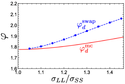
Figure 4: Phase diagram of the binary MK model. The solid red line denotes the dynamical transition point of the standard MC. The filled blue symbols with the dashed line denote the dynamical transition points of the swap MC. The blue dashed line is an eye guide.

From Eqs. (31), we can calculate the dynamical transition point. The results are summarized in Fig. 4. As expected, the dynamical transition point of the standard and swap MC are the same when the size ratio is unity. The difference between $\varphi_{d}^{\rm mc}$ and $\varphi_{d}^{\rm swap}$ becomes larger with increasing the size ratio. Note however that, in Eq. (15), we assume that the cage size is independent from the particle species. This assumption would be inappropriate when the size ratio becomes very large: we discuss in the Appendix a more general ansatz with two different cages, one for each type of particles.

VI Computer simulations

VI.1 Methods

In this section, we perform computer simulations of the binary MK model and compare the results with the theoretical predictions discussed in Sec. V. We employ standard MC and swap MC simulations for the equimolar binary MK model in $d=3$. The number of large and small particles are $N_{L}=500$ and $N_{S}=500$, respectively. In case of the standard MC, we randomly choose a particle and try to shift the particle position as $(x,y,z)\to(x+\varepsilon r_{x},y+\varepsilon r_{y},z+\varepsilon r_{z})$, where $r_{\alpha}$ is a random number uniform in $[-1,1]$ and $\varepsilon$ is an algorithm parameter. We fix $\varepsilon=0.25$ in this simulation. We accept the new position if the particle shifted in the new position does not overlap with any other particle. For the swap MC, in addition to the shift of the particle position, we try to swap the sizes of particles. We randomly choose two particles $i$ and $j$, and try to exchange their sizes; note that each particle keeps its label (i.e. particle $i$ remains $i$ and $j$ remains $j$) and its random shifts (otherwise the move would never be accepted), but the sizes of the two particles are exchanged (i.e. particle $i$ now has the diameter of $j$, and viceversa). We accept this trial move if there are no overlapped particles in the new configuration. We try to shift the positions with probability $1-\alpha$ and to swap the sizes with probability $\alpha$. As in Ref. Berthier et al. (2016), we set $\alpha=0.2$. We prepare initial equilibrated configurations by using the planting method, which in the MK model allows one to obtain perfectly equilibrated configurations even beyond $\varphi_{d}$ Mari and Kurchan (2011); Charbonneau et al. (2014). Below, we report the results for $\sigma_{LL}/\sigma_{SS}=1.4$. We have confirmed that the qualitative behavior is unchanged for different values of the size ratio.

VI.2 Self-correlation function and relaxation time

The first observable that we investigate is the self-correlation function, which characterizes the slow motion of the particle positions Hansen and McDonald (1990):

$$F_{s}(k,t) =\sum_{i=1}^{N}\frac{1}{N}\left\langle e^{i\bm{k}\cdot(\bm{x}_{i}(t)-\bm{x}_{i}(0))}\right\rangle,$$ (32)

where $\bm{k}$ denotes the wave vector. Because the system is isotropic, $F_{s}(k,t)$ is a function of the absolute value of $\bm{k}$. Following Ref. Mari and Kurchan (2011), we set $k=\left|\bm{k}\right|=\pi$. In Fig. 5, we plot $F_{s}(k,t)$ obtained by the computer simulation as a function of the MC step, where one MC step is defined as $N$ MC trials. At very low densities, the relaxation time of the standard and swap MC are compatible. On the contrary, at higher $\varphi$, $F_{s}(k,t)$ of the swap MC seems to relax faster than that of the standard MC.

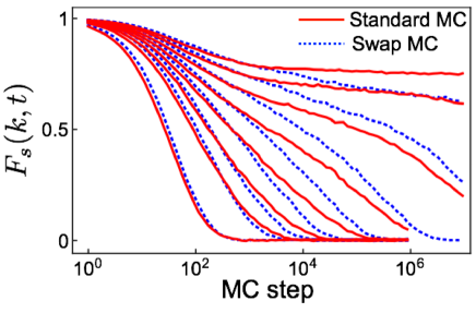
Figure 5: Equilibrium self-correlation function of the binary MK model. The red solid lines denote the results of the standard MC, while the blue dashed lines denote the results of the swap MC. $\varphi=0.5,1.0,1.2,1.4,1.6,1.8,2.0,2.2$ from left to right.

From $F_{s}(k,t)$, we define the relaxation time, $\tau_{\alpha}$, by $F_{s}(k,\tau_{\alpha})=1/e$. The resulting values of $\tau_{\alpha}$ calculated by the computer simulation are reported in Fig. 6. To compare with the theoretical prediction, we fit the numerical data by the power law function predicted by the MCT Gotze (2009):

$$\tau_{\alpha}=\tau_{0}(\varphi_{d}-\varphi)^{-\gamma},$$ (33)

where $\varphi_{d}$ is not a fitting parameter, as it is determined by our theory described in Sec. V. The precise values of $\varphi_{d}$ for the standard and swap MC are $\varphi_{d}^{\rm mc}=1.87$ and $\varphi_{d}^{\rm swap}=2.02$, respectively. $\tau_{0}$ and $\gamma$ are fitting parameters. The result of the fitting is shown in Fig. 6 with solid lines. We also show the MCT scaling plot in the inset. The scaling formula Eq. (33) works well for a wide range of relaxation times, but, for very large values of the relaxation time ($\tau_{\alpha}>10^{6}$), the MCT fit systematically overestimates the relaxation time both for the standard and swap MC. This is a natural result because, in finite dimension, the dynamical transition of the MK model is avoided due to rare hopping events Charbonneau et al. (2014).

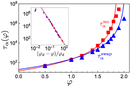
Figure 6: $\varphi$ dependence of the equilibrium relaxation time of the binary MK model. The filled red squares and filled blue triangles denote the result obtained by the computer simulation of the standard and swap MC, respectively. The solid lines indicate the theoretical prediction. (Inset) Scaling plot of the same data of the main panel.

VI.3 Long time limit of physical quantities

In this subsection, we compare the physical quantities in the long time limit calculated by theory and computer simulations. We first observe the MSD defined by Eq. (1). In Fig. 7(a), we show the equilibrium ${\rm MSD}$ calculated by the computer simulation. At small $\varphi$, the ${\rm MSD}$ continues to grow with time and diverges in the long time limit. Contrary, at large $\varphi$, the ${\rm MSD}$ saturates and converges to a finite value in the long time limit, meaning that particles are trapped in a narrow region, the “cage”. Using the Gaussian ansatz, Eq. (16), one can show that the long time value is related to the cage size, $A$, by

$$\lim_{t\to\infty}{\rm MSD}(t) =2dA.$$ (34)

We approximate the long time limit by the value of ${\rm MSD}(t)$ at $t=10^{7}$ and plot the result with the theoretical prediction, see Fig. 7(b). The results of the computer simulation (filled symbols) and theoretical prediction (solid lines) are consistent at large $\varphi$. However, for small $\varphi$, the theory underestimates the cage size, as already observed in Charbonneau et al. (2014). Part of this discrepancy comes from the poor approximations used in our theory. In Appendix, we show that one can obtain a better result by improving the molecular density approximation, Eq. (15).

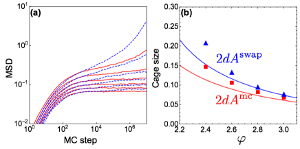
Figure 7: (a) Equilibrium mean square displacement of the binary MK model. The red solid and blue dashed lines denote the result of the standard and swap MC, respectively. $\varphi=2.0,2.2,2.4,2.6,2.8,3.0$ from top to bottom. (b) $\varphi$ dependence of the cage size (long time limit of the MSD). The filled red squares and blue triangles denote the numerical results of the standard and swap MC, respectively. The theoretical result is shown as a solid line of the same color.

In the swap MC, the particle species changes with time. The slow dynamics related to this motion is characterized by

$$q(t) \equiv\frac{1}{N}\sum_{i=1}^{N}\left\langle\sigma_{i}(t)\sigma_{i}(0)\right\rangle,$$ (35)

where $\sigma_{i}(t)=1$ if the $i$-th particle is a large particle at time $t$, otherwise $\sigma_{i}(t)=-1$. In Fig. 8(a), we show $q(t)$ calculated by computer simulations for several values of $\varphi$ as a solid line. We also show $F_{s}(k,t)$ as a dashed line. One can see that the relaxation time of $q(t)$ is comparable to that of $F_{s}(k,t)$. This is consistent with the theoretical prediction that the order parameters of the position and species begin to have finite values at the same density as shown in Fig. 3.

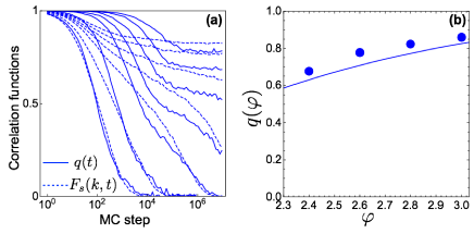
Figure 8: (a) Equilibrium correlation functions of the swap MC. The solid line denotes $q(t)$ and the dashed line denotes $F_{s}(k,t)$. $\varphi=1.0,1.4,1.8,2.0,2.2,2.4,2.6$ from left to right. (b) $\varphi$ dependence of $q(\varphi)$. The blue filled circle denotes the numerical data. The blue solid line denotes the theoretical prediction.

Above $\varphi_{d}^{\rm swap}$, the mean-field theory predicts that $q(t)$ does not decay to zero and converges to a finite value:

$$\lim_{t\to\infty}q(t)=\left\langle\sigma(\mu^{a})\sigma(\mu^{b})\right\rangle=q.$$ (36)

where $q$ is calculated by the $m\to 1$ limit of Eq. (19). Instead of the long time limit, we evaluate $q(t)$ at $t=10^{7}$ MC step and compare with the theoretical prediction. The result is summarized in Fig. 8(b). The agreement is good given the simplicity of the approximation. One can obtain a better result by improving the ansatz, see the Appendix.

VII Configurational entropy, thermodynamic glass transition point, and activated dynamics

In this section, we discuss the behavior of the configurational entropy, the thermodynamic glass transition point and the activated dynamics. Unfortunately, the intensive free energy of the MK model diverges in the thermodynamic limit, $N\to\infty$, and we can not discuss the thermodynamic glass transition of this model Mari and Kurchan (2011). Here instead, we discuss the qualitative predictions of our theory for more realistic glass forming systems. More explicitly, we consider standard three-dimensional binary or polydisperse mixtures of repulsive particles, such as the ones discussed in Ninarello et al. (2017), though our discussion may apply to a broader range of systems.

VII.1 Configurational entropy

The RFOT scenario and the associated RLT generically (but with notable exceptions Berthier et al. (2011)) predict that the thermodynamic glass transition point, $\varphi_{K}$, exists at a higher density than the dynamic transition density $\varphi_{d}$. The configurational entropy $S_{\rm conf}$ characterizes the proximity to the thermodynamic glass transition point, which is defined by $S_{\rm conf}=S_{\rm liq}-S_{\rm glass}$, where $S_{\rm liq}$ and $S_{\rm glass}$ are the entropies of the liquid and glass, respectively. In the liquid phase, $S_{\rm liq}>S_{\rm glass}$ and $S_{\rm conf}>0$. With increasing $\varphi$, $S_{\rm conf}$ decreases and eventually vanishes at $\varphi_{K}$.

However in binary or polydisperse mixtures, our theory provides two different configurational entropies corresponding to the two different ansatzes discussed above. Note that approximate analytical calculations of $S_{\rm conf}$ for realistic three-dimensional systems could be performed using the two ansatzes, following e.g. the scheme developed in Mangeat and Zamponi (2016). We leave this for future work, and here we limit ourselves to a schematic discussion of the expected result. In Fig. 9, we show the expected behavior of $S_{\rm conf}$ calculated by the ansatz corresponding to the standard MC, $S_{\rm conf}^{\rm mc}$, and that corresponding to the swap MC, $S_{\rm conf}^{\rm swap}$.

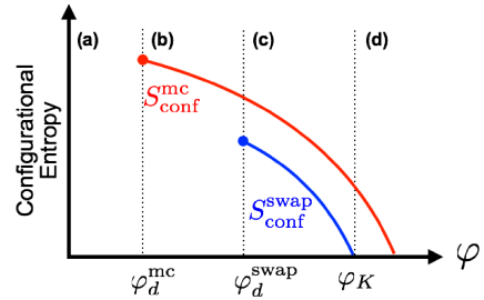
Figure 9: Schematic behavior of the configurational entropy.

$S_{\rm conf}^{\rm mc}$ and $S_{\rm conf}^{\rm swap}$ are well defined only above $\varphi_{d}^{\rm mc}$ and $\varphi_{d}^{\rm swap}$, respectively. In general, $S_{\rm conf}^{\rm swap}<S_{\rm conf}^{\rm mc}$ because the glass entropy $S_{\rm glass}$ associated to the swap MC is higher than that of the standard MC; this is due to the additional degrees of freedom related to the particle exchange, which is only allowed in the swap MC. Thus, two different thermodynamic glass transition points $\varphi_{K}$ are obtained from our theory. The one calculated by $S_{\rm conf}^{\rm mc}$ is higher than that of $S_{\rm conf}^{\rm swap}$.

From a purely thermodynamic point of view, the standard MC ansatz does not have a real meaning. In fact, thermodynamically one seeks to minimize the free energy over the whole space of functions $\rho_{\overline{\mu}}(\overline{\bm{x}})$, and the swap MC ansatz gives a lower free energy solution which thus dominates the partition function and the free energy. The metastable glassy states in the standard MC ansatz can be interpreted as an artifact due to the kinetic constraint that prohibits the exchange of particles of different species. Thus, the thermodynamic glass transition point should be determined by $S_{\rm conf}^{\rm swap}(\varphi_{K})=0$, or even better, $\varphi_{K}$ should be determined by the full optimization of the replicated free energy, i.e. using the most general ansatz for $\rho_{\overline{\mu}}(\overline{\bm{x}})$.

Note that a similar issue in the definition of the configurational entropy also appears in computer simulation studies. One should take into account the exchange of particle species when calculating the entropy of the glass state (or the vibrational entropy in the terminology of the computer simulations and experiments), otherwise one would overestimate the value of the configurational entropy. The methods proposed so far seem still inappropriate for this purpose. For instance, the inherent structure method Scala et al. (2000); Sciortino et al. (1999) and the Frenkel-Ladd method Angelani and Foffi (2007) take into account only the vibrational motion around the equilibrium position and neglect the exchange of the particle species when calculating the entropy of the glass state. A generalization of these methods to take into account exchange has been discussed recently in Ozawa and Berthier (2017). Another approach based on spin glass theory Franz and Parisi (1997) has been proposed by Berthier and Coslovich Berthier and Coslovich (2014): using the umbrella sampling, they calculated the free energy as a function of an overlap order parameter associated to the particle positions, which partially allows for particle exchanges. A comparison of the two methods, however, still reveals discrepancies Berthier et al. (2017), which might be due to the approximations involved. A complete treatment of the configurational entropy in computer simulations is left for future work.

VII.2 Activated dynamics

We now discuss the consequences of this structure for the dynamics, but we warn the reader that the discussion of this subsection is highly speculative.

From a dynamical point of view, the solution obtained from the standard MC ansatz might have an important meaning. The RFOT theory claims that above the dynamical transition point, the free energy has many metastable states whose lifetime is controlled by the configurational entropy Kirkpatrick et al. (1989); Bouchaud and Biroli (2004). The theory suggests that in finite dimensional systems, after an initial slowing down controlled by the MCT scaling in Eq. (33), the dynamical transition is avoided and activated dynamics sets in, leading to the following Adam-Gibbs relation:

$$\log\tau_{\alpha}\propto S_{\rm conf}^{-\eta},$$ (37)

where the critical exponent $\eta$ depends on the shape of the activated region Bouchaud and Biroli (2004). Eq. (37) predicts that a divergence of the relaxation time is concomitant to the vanishing of $S_{\rm conf}$. For the swap dynamics, the standard RFOT scenario could apply, using the configurational entropy $S_{\rm conf}^{\rm swap}$, with the usual caveats and limitations discussed extensively in Biroli and Bouchaud (2012).

However, in order to apply RFOT arguments to the standard MC, one should take into account the existence of an additional local time scale $\tau_{\rm ex}(T,\varphi)$ that controls particle exchange. If $\tau_{\rm ex}$ were to be infinite, then one could apply to the standard MC the usual RFOT arguments leading to an Adam-Gibbs relation controlled by $S_{\rm conf}^{\rm mc}$. However, because of its local nature, the time scale $\tau_{\rm ex}$ cannot diverge at any finite temperature. Therefore, upon lowering temperature, at some point one will necessarily have

$$\log\tau^{\rm mc}_{\alpha}\propto(S_{\rm conf}^{\rm mc})^{-\eta}\gg\log\tau_{\rm ex}\ .$$ (38)

When this happens, exchange becomes much faster than the lifetime of the metastable states that dominate $S_{\rm conf}^{\rm mc}$, revealing their instability against exchange. This argument reveals that there must be a temperature $T_{\rm ex}$ below which (or a density $\varphi_{\rm ex}$ above which) $S_{\rm conf}^{\rm mc}$ looses its dynamical meaning (we have already seen that it has no thermodynamical meaning). Below $T_{\rm ex}$ (above $\varphi_{\rm ex}$), the standard MC cannot follow anymore the Adam-Gibbs relation associated to $S_{\rm conf}^{\rm mc}$, and a different dynamics must set in, controlled either by the local exchange processes, or by the Adam-Gibbs relation associated to the swap dynamics, depending on how the two processes interact. Note that $T_{\rm ex}$ is expected to be strongly system-dependent due to the local nature of $\tau_{\rm ex}$, which depends on the details of the local particle caging. Note also that $\tau_{\rm ex}$ exists even in the $3d$ MK model Charbonneau et al. (2014).

One could well imagine a situation in which $\tau_{\rm ex}$ is small enough that it destabilizes the whole curve $S_{\rm conf}^{\rm mc}$, i.e. $T_{\rm ex}>T_{d}^{\rm mc}$ or $\varphi_{\rm ex}<\varphi_{d}^{\rm mc}$. In this case, in finite dimensions the finite lifetime of the states associated to $S_{\rm conf}^{\rm mc}$ would be determined by single particle hopping out of the cage Berthier et al. (2004); Candelier et al. (2010); Keys et al. (2011); Charbonneau et al. (2014); Ciamarra et al. (2016), rather than by RFOT-like collective phenomena. In this scenario, one might therefore expect that the beginning of the slow dynamics in the region $\varphi_{d}^{\rm mc}<\varphi<\varphi_{d}^{\rm swap}$ would be associated to a local hopping effect, as in the DFT scenario Ritort and Sollich (2003); Chandler and Garrahan (2010); Biroli and Garrahan (2013), while around $\varphi_{d}^{\rm swap}$ a crossover to the RFOT scenario would be observed, as also discussed in Wyart and Cates (2017). Note that the precise relation between the hopping kinetic constraint considered above and the one assumed in the DFT is not clear. Finally, systems with shorter hopping timescales would exhibit a smaller window of single-particle slow dynamics before the crossover to the RFOT regime is reached. More work is necessary to uncover the precise mechanisms of the slow dynamics in the region $\varphi_{d}^{\rm mc}<\varphi<\varphi_{d}^{\rm swap}$.

VIII Summary and discussion

In this work, we constructed a new ansatz for the replica liquid theory so as to separately calculate the dynamical glass transition points of the swap and standard Monte Carlo algorithms within the mean field RFOT scenario. This is possible by taking into account the effect of the exchange of particle species. We applied the theory to the binary Mari-Kurchan (MK) model and calculated the dynamical transition points of the swap and standard MC, $\varphi_{d}^{\rm swap}$ and $\varphi_{d}^{\rm mc}$, respectively. We also performed standard and swap MC simulations of the binary MK model and quantitatively showed that the dynamics in the standard MC simulation is dominated by $\varphi_{d}^{\rm mc}$, while that in the swap MC simulation is dominated by $\varphi_{d}^{\rm swap}$, thus validating our ansatzes.

We also discussed qualitatively the thermodynamics and dynamics of more realistic glass forming systems, as expected from our theory; concrete calculations could be performed in the future for these systems through a straightforward extension of the theory. Four distinct density (or temperature) regions exist, see Fig. 9. (a) When $\varphi<\varphi_{d}^{\rm mc}$, the relaxation time of the standard and swap MC are both small, and the system is liquid. (b) When $\varphi_{d}^{\rm mc}<\varphi<\varphi_{d}^{\rm swap}$, there are glassy metastable states that are stable only if particle exchange is forbidden. Therefore, if one uses the swap MC, the system relaxes as fast as in the liquid. Conversely, if one uses the standard MC, the system displays slow dynamics due to the kinetic constraint that prohibits the exchange of particles species. (c) When $\varphi_{d}^{\rm swap}<\varphi<\varphi_{K}$, there are glassy metastable states in the free energy that remain stable even if particle exchange is allowed. At the mean field level, the system is trapped in a metastable state both for the standard and swap MC, while in finite dimensions the RFOT scenario should be applicable, and activated relaxation should dominate the dynamics in both cases. Note that when the lifetime of the metastable states overcomes the typical time scale to exchange particles of different species, the relaxation times of the standard and swap MC would become comparable. In both cases, the relaxation time diverges upon approaching $\varphi_{K}$. (d) When $\varphi>\varphi_{K}$, the thermodynamic glass transition takes place and the system loses the ergodicity, remaining arrested in an ideal glass phase.

It is worth mentioning that, with the appropriate re-scaling, the slow dynamics of the standard MC is essentially the same as that of other more realistic dynamics such as the Langevin dynamics, Brownian dynamics, Newtonian dynamics, and possibly, the true experimental dynamics Gleim et al. (1998); Szamel and Flenner (2004); Berthier and Kob (2007). Thus, our results should be translated straightforwardly to these dynamics, provided the system under investigation is reasonably close to being mean field, in the sense of a Ginzburg criterion Franz et al. (2012). The latter property is strongly system-dependent, and in many systems the mean field scenario can be heavily affected by finite dimensional fluctuations. In particular, it is well known that the dynamical transition points $\varphi_{d}^{\rm mc}$ and $\varphi_{d}^{\rm swap}$ become simple crossovers in finite dimensional systems Biroli and Bouchaud (2012).

Keeping in mind these limitations, our results raise several interesting points for discussion.

• In Sec. VII.2, we argued that in one possible scenario, the exchange time $\tau_{\rm ex}$ is smaller than the Adam-Gibbs lifetime of the states associated to $S_{\rm conf}^{\rm mc}$ already around $\varphi_{d}^{\rm mc}$. In this case, $S_{\rm conf}^{\rm mc}$ would not control the slow dynamics. One first observes a slowdown dominated by the local exchange process, and then a crossover to RFOT-like dynamics in presence of exchange, which would be associated to $S_{\rm conf}^{\rm swap}$. A similar conclusion has been obtained in the work of Wyart and Cates Wyart and Cates (2017). They claim that around the (experimental) glass transition point $\varphi_{g}$, the local activation energy $E_{\rm loc}$, which describes the local physics and cannot diverge, is much larger than the collective activation energy $E_{\rm cor}$, which is controlled by the growing static length scale predicted by the RFOT scenario and diverges at the thermodynamic glass transition point $\varphi_{K}$ ( or $T_{K}$). From this assumption, they concluded that the slow dynamics of realistic systems is not related to the existence of metastable states Wyart and Cates (2017). We consider that the static length scale or $E_{\rm cor}$ is controlled by $S_{\rm conf}^{\rm swap}$ because $S_{\rm conf}^{\rm mc}$ is meaningless from the thermodynamic point of view as we discussed in Sec. VII.1. Thus, Wyart and Cates assumption $E_{\rm loc}\gg E_{\rm cor}$ is equivalent to assume that $\varphi_{g}$ is lower than the density at which a crossover to RFOT-like dynamics associated to $S_{\rm conf}^{\rm swap}$ takes place.

• The scenario outlined above, i.e. the fact that the relaxation of the standard MC dynamics is dominated by local exchange processes is peculiar, almost by definition, to systems for which the swap MC dynamics is efficient. In other words, one should keep in mind that the class of models investigated in Ninarello et al. (2017), for which the swap algorithm provides a speedup of many orders of magnitude, could be a specific class of glassy systems for which relaxation is dominated by local exchange processes. Other glassy systems could behave differently and present a truly cooperative relaxation. For example, for one-component or nearly one-component glass forming systems such as the Gaussian core model Ikeda and Miyazaki (2011), the dynamical transition points of the standard and swap MC are obviously identical and the region (b) where the slow dynamics is controlled by the kinetic constraint disappears. Those models could then display cooperative relaxation and could thus be ideal playgrounds to test the validity of the RFOT scenario.

• For systems where the swap algorithm is efficient, and $\varphi_{d}^{\rm mc}<\varphi_{d}^{\rm swap}$, within our mean field framework, we expect that the standard MC dynamics should exhibit a mode-coupling like phenomenology upon approaching $\varphi_{d}^{\rm mc}$, as usual, but the swap MC should also exhibit MCT-like phenomenology upon approaching $\varphi_{d}^{\rm swap}$ (of course both transitions would be avoided in finite dimensions due to activated processes). In other words, one expects that the swap MC should develop dynamical heterogeneities, a critical MCT scaling of the approach to and departure from the plateau, etc. Some of these phenomena are indeed observed in Ninarello et al. (2017), but a more systematic study should be performed.

• Because the swap MC should become arrested around $\varphi_{d}^{\rm swap}$, i.e. before the metastable states associated to $S_{\rm conf}^{\rm swap}$ are able to develop, this would not be an efficient algorithm to sample such states. In particular, the configurational entropy measured in Berthier et al. (2017) likely pertains to the region $\varphi_{d}^{\rm mc}<\varphi<\varphi_{d}^{\rm swap}$, i.e. region (b) above, which is the only one accessible to the swap MC. The configurational entropy $S_{\rm conf}^{\rm swap}$ is not well defined in that region, and therefore its measurement could be plagued by ambiguities, due to the fact that these states have a finite (and possibly not so long) lifetime in that region. This is likely to impact in particular the measurements made via the Frenkel-Ladd method, which requires states to be stable for long times, while measurement made through the Franz-Parisi potential should be more reliable Berthier and Coslovich (2014).

• Finally, our work shows that even in a region where the slow dynamics is completely dominated by local kinetic constraints, one can construct an appropriate thermodynamic theory (in our case, by forbidding particle exchanges in the construction of replicated molecules) that is able to capture the associated metastability; a similar example can be found in Ref. Foini et al. (2012).

We are therefore convinced that our work raises a number of interesting questions that will hopefully be addressed by future analytical and numerical works.

Appendix: Two-cage Ansatz

In this Appendix, we construct a more general ansatz than the decoupling approximation in Eq. (15). We allow the cage size to depend on the particles species and make the following ansatz:

$$\rho_{\overline{\mu}}(\overline{\bm{x}}) =\rho(\overline{\bm{x}}|\overline{\mu})g(\overline{\mu}),$$ (39)

where $g(\overline{\mu})$ is defined by Eq. (17) and

$$\rho(\overline{\bm{x}}|\overline{\mu})=\rho\int d\bm{X}\prod_{a=1}^{m}\gamma_{A_{\sigma^{a}}}(\bm{x}^{a}-\bm{X})=\frac{\rho}{\prod_{a=1}^{m}\left(2\pi A_{\sigma^{a}}\right)^{d/2}}\left(\frac{2\pi}{\sum_{a=1}^{m}A_{\sigma^{a}}^{-1}}\right)^{d/2}\exp\left[-\frac{1}{4\sum_{a=1}^{m}A_{\sigma^{a}}^{-1}}\sum_{ab}\frac{(\bm{x}^{a}-\bm{x}^{b})^{2}}{A_{\sigma^{a}}A_{\sigma^{b}}}\right].$$ (40)

Here we used the shorthand notation, $\sigma^{a}=\sigma(\mu^{a})$. $A_{L}$ and $A_{S}$ are the cage sizes of large and small particles, respectively. Hereafter, we call this the “two-cage ansatz”, while we refer to the ansatz in the main text as the “one-cage ansatz”. Substituting the above ansatz into the free energy Eq. (12), we obtain

$$\frac{\log Z_{m}}{N} =S_{id}^{x}+S_{id}^{\sigma}+S_{int}+\log N,$$

$$S_{id}^{\sigma} =\log\int Dh\left(2\cosh(h)\right)^{m}-\frac{\Delta^{2}}{2}\left(m+m(m-1)\frac{\int Dh\cosh(h)^{m}\tanh(h)^{2}}{\int Dh\cosh(h)^{m}}\right),$$

$$S_{id}^{x} =-\log\rho+\frac{d}{4}m(\log A_{L}+\log A_{S})+(m-1)\frac{d}{2}\log(2\pi)+(m-1)\frac{d}{2}$$

$$+\frac{d}{2}\int_{0}^{\infty}\frac{dt}{t}\left[e^{-t}-\frac{1}{\int Dh(2\cosh(h))^{m}}\int Dh\left(e^{h-t/A_{L}}+e^{-h-t/A_{S}}\right)^{m}\right],$$

$$S_{int} =\frac{\rho}{2}\int d\bm{r}\left(\frac{1}{C_{m}^{2}}\int DuDvq(r,u,v)^{m}-1\right),$$

$$q(r,u,v) =\sum_{\mu\nu}e^{u\sigma(\mu)+v\sigma(\nu)}\int d\bm{u}\gamma_{A_{\sigma(\mu)}+A_{\sigma(\nu)}}(r+u)e^{-\beta v_{\mu\nu}(u)}.$$ (41)

The order parameters are calculated by the saddle point conditions, $\partial_{A_{L}}\log Z_{m}=0$, $\partial_{A_{S}}\log Z_{m}=0$, and $\partial_{\Delta}\log Z_{m}=0$. After some manipulations, we obtain the following self-consistent equations:

$$A_{L} =M_{L}(A_{L},A_{S},\Delta),$$

$$A_{S} =M_{S}(A_{L},A_{S},\Delta),$$

$$\Delta =M_{\Delta}(A_{L},A_{S},\Delta),$$ (42)

where

$$M_{L}(A_{L},A_{S},\Delta) =\frac{\frac{d}{4}+\frac{d}{2}\int_{0}^{\infty}\frac{dt}{A_{L}}e^{-t/A_{L}}\left[\frac{f}{4}-\frac{K_{L}}{2}\right]}{-\frac{\rho}{8}e^{-\Delta^{2}}\int drDhDh^{\prime}\frac{\partial q}{\partial A_{L}}\left(\log q-f\right)},$$

$$M_{S}(A_{L},A_{S},\Delta) =\frac{\frac{d}{4}+\frac{d}{2}\int_{0}^{\infty}\frac{dt}{A_{S}}e^{-t/A_{S}}\left[\frac{f}{4}-\frac{K_{S}}{2}\right]}{-\frac{\rho}{8}e^{-\Delta^{2}}\int drDhDh^{\prime}\frac{\partial q}{\partial A_{S}}\left(\log q-f\right)},$$

$$M_{\Delta}(A_{L},A_{S},\Delta) =-\frac{1}{1+q}\Bigg{[}-\frac{f^{\prime}}{2}+\frac{\Delta^{2}}{2}g^{\prime}-\frac{d}{2}\int\frac{dt}{t}\left[\frac{f^{\prime}}{2}\frac{e^{-t/A_{l}}+e^{-t/A_{S}}}{2}\frac{K^{\prime}}{2}\right]$$

$$+\frac{\rho}{4}\Delta e^{-\Delta^{2}}\int q(\log q-f)-\frac{\rho}{8}e^{-\Delta^{2}}\int dr\frac{\partial Dh}{\partial\Delta}Dh^{\prime}q(\log q-f)-\frac{\rho}{8}e^{-\Delta^{2}}\int drDh\frac{\partial Dh^{\prime}}{\partial\Delta}q(\log q-f)$$

$$+\frac{\rho}{8}e^{-\Delta^{2}}\int qf^{\prime}\Bigg{]}.$$ (43)

We have introduced the auxiliary functions, $K$, $K_{L}$ and $K_{S}$ as

$$K(A_{L},A_{S},\Delta) =e^{-\Delta^{2}/2}\int Dh\left(e^{h-t/A_{L}}+e^{-h-t/A_{S}}\right)\log\left(e^{h-t/A_{L}}+e^{-h-t/A_{S}}\right),$$

$$K_{L}(A_{L},A_{A},\Delta) =1+e^{-\Delta^{2}/2}\int Dhe^{h}\log\left(e^{h-t/A_{L}}+e^{-h-t/A_{S}}\right),$$

$$K_{S}(A_{L},A_{S},\Delta) =1+e^{-\Delta^{2}/2}\int Dhe^{-h}\log\left(e^{h-t/A_{L}}+e^{-h-t/A_{S}}\right).$$ (44)

We solved the self-consistent equations by using the iterative method for the size ratio $\sigma_{LL}/\sigma_{SS}=1.4$. The result is summarized in Fig. 10. One can see that the two cage ansatz gives a slightly better result than the one-cage ansatz at this size ratio. Our preliminary calculations for smaller size ratio $\sigma_{LL}/\sigma_{SS}\approx 1.2$ predict, however, a decoupling of the glass transition point of the position and species, which was never observed in computer simulation. The reason for this discrepancy between the theory and computer simulations is still unclear and its clarification is left for future work.

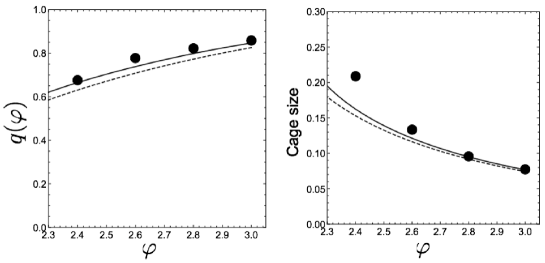
Figure 10: Order parameters of the swap MC for $\sigma_{LL}/\sigma_{SS}=1.4$. The filled symbols denote the results obtained by the computer simulation. The solid line denotes the result of the two-cage ansatz. The dashed line denotes the result of the one-cage ansatz.

References

- Debenedetti and Stillinger (2001) P. G. Debenedetti and F. H. Stillinger, Nat. 410, 259 (2001).
- Cavagna (2009) A. Cavagna, Phys. Rep. 476, 51 (2009).
- Gotze (2009) W. Gotze, Complex dynamics of glass-forming liquids (Oxford University Press, 2009).
- Berthier and Biroli (2011) L. Berthier and G. Biroli, Rev. Mod. Phys. 83, 587 (2011).
- Biroli and Garrahan (2013) G. Biroli and J. P. Garrahan, J. Chem. Phys. 138, 12A301 (2013).
- Kirkpatrick and Wolynes (1987) T. Kirkpatrick and P. Wolynes, Phys. Rev. A 35, 3072 (1987).
- Kirkpatrick et al. (1989) T. Kirkpatrick, D. Thirumalai, and P. G. Wolynes, Phys. Rev. A 40, 1045 (1989).
- Bouchaud and Biroli (2004) J.-P. Bouchaud and G. Biroli, J. Chem. Phys. 121, 7347 (2004).
- Lubchenko and Wolynes (2007) V. Lubchenko and P. G. Wolynes, Annu. Rev. Phys. Chem. 58, 235 (2007).
- Kirkpatrick and Thirumalai (2015) T. R. Kirkpatrick and D. Thirumalai, Rev. Mod. Phys. 87, 183 (2015).
- Parisi and Zamponi (2010) G. Parisi and F. Zamponi, Rev. Mod. Phys. 82, 789 (2010).
- Charbonneau et al. (2017) P. Charbonneau, J. Kurchan, G. Parisi, P. Urbani, and F. Zamponi, Annu. Rev. Condens. Matter Phys. 8, 265 (2017).
- Mézard and Parisi (1999a) M. Mézard and G. Parisi, J. Phys. Condens. Matter 11, A157 (1999a).
- Mézard and Parisi (1999b) M. Mézard and G. Parisi, J. Chem. Phys. 111, 1076 (1999b).
- Parisi and Zamponi (2005) G. Parisi and F. Zamponi, J. Chem. Phys. 123, 144501 (2005).
- Jacquin et al. (2011) H. Jacquin, L. Berthier, and F. Zamponi, Phys. Rev. Lett. 106, 135702 (2011).
- Berthier et al. (2011) L. Berthier, H. Jacquin, and F. Zamponi, Phys. Rev. E 84, 051103 (2011).
- Mangeat and Zamponi (2016) M. Mangeat and F. Zamponi, Phys Rev. E 93, 012609 (2016).
- Bengtzelius et al. (1984) U. Bengtzelius, W. Gotze, and A. Sjolander, J. Phys. C 17, 5915 (1984).
- Maimbourg et al. (2016) T. Maimbourg, J. Kurchan, and F. Zamponi, Phys. Rev. Lett. 116, 015902 (2016).
- Adam and Gibbs (1965) G. Adam and J. H. Gibbs, J. Chem. Phys. 43, 139 (1965).
- Kauzmann (1948) W. Kauzmann, Chem. Rev. 43, 219 (1948).
- (23) G. Biroli, J.-P. Bouchaud, A. Cavagna, T. S. Grigera, and P. Verrocchio, Nat. Phys. 4, 771.
- Berthier and Kob (2012) L. Berthier and W. Kob, Phys. Rev. E 85, 011102 (2012).
- Cammarota and Biroli (2012) C. Cammarota and G. Biroli, PNAS 109, 8850 (2012).
- Cammarota and Biroli (2013) C. Cammarota and G. Biroli, J. Chem. Phys. 138, 12A547 (2013).
- Karmakar and Parisi (2013) S. Karmakar and G. Parisi, PNAS 110, 2752 (2013).
- Kob and Berthier (2013) W. Kob and L. Berthier, Phys. Rev. Lett. 110, 245702 (2013).
- Ozawa et al. (2015) M. Ozawa, W. Kob, A. Ikeda, and K. Miyazaki, PNAS 112, 6914 (2015).
- Ritort and Sollich (2003) F. Ritort and P. Sollich, Adv. Phys. 52, 219 (2003).
- Chandler and Garrahan (2010) D. Chandler and J. P. Garrahan, Annu. Rev. Phys. Chem. 61, 191 (2010).
- Keys et al. (2011) A. S. Keys, L. O. Hedges, J. P. Garrahan, S. C. Glotzer, and D. Chandler, Phys. Rev. X 1, 021013 (2011).
- Isobe et al. (2016) M. Isobe, A. S. Keys, D. Chandler, and J. P. Garrahan, Phys. Rev. Lett. 117, 145701 (2016).
- Fredrickson and Andersen (1984) G. H. Fredrickson and H. C. Andersen, Phys. Rev. Lett. 53, 1244 (1984).
- Sellitto et al. (2005) M. Sellitto, G. Biroli, and C. Toninelli, EPL 69, 496 (2005).
- Sellitto et al. (2010) M. Sellitto, D. De Martino, F. Caccioli, and J. J. Arenzon, Phys. Rev. Lett. 105, 265704 (2010).
- Ikeda and Miyazaki (2015) H. Ikeda and K. Miyazaki, EPL 112, 16001 (2015).
- Sellitto (2015) M. Sellitto, Phys. Rev. Lett. 115, 225701 (2015).
- De Candia et al. (2016) A. De Candia, A. Fierro, and A. Coniglio, Sci. Rep. 6, 26481 (2016).
- Ikeda et al. (2017) H. Ikeda, K. Miyazaki, and G. Biroli, EPL 116, 56004 (2017).
- Berthier et al. (2012) L. Berthier, G. Biroli, D. Coslovich, W. Kob, and C. Toninelli, Phys. Rev. E 86, 031502 (2012).
- Wyart and Cates (2017) M. Wyart and M. E. Cates, Phys. Rev. Lett. 119, 195501 (2017).
- Gazzillo and Pastore (1989) D. Gazzillo and G. Pastore, Chem. Phys. Lett. 159, 388 (1989).
- Grigera and Parisi (2001) T. S. Grigera and G. Parisi, Phys. Rev. E 63, 045102 (2001).
- Cavagna et al. (2012) A. Cavagna, T. S. Grigera, and P. Verrocchio, J. Chem. Phys. 136, 204502 (2012).
- Gutiérrez et al. (2015) R. Gutiérrez, S. Karmakar, Y. G. Pollack, and I. Procaccia, EPL 111, 56009 (2015).
- Berthier et al. (2016) L. Berthier, D. Coslovich, A. Ninarello, and M. Ozawa, Phys. Rev. Lett. 116, 238002 (2016).
- Ninarello et al. (2017) A. Ninarello, L. Berthier, and D. Coslovich, Phys. Rev. X 7, 021039 (2017).
- Berthier et al. (2017) L. Berthier, P. Charbonneau, D. Coslovich, A. Ninarello, M. Ozawa, and S. Yaida, PNAS , 201706860 (2017).
- Mari and Kurchan (2011) R. Mari and J. Kurchan, J. Chem. Phys. 135, 124504 (2011).
- Charbonneau et al. (2014) P. Charbonneau, Y. Jin, G. Parisi, and F. Zamponi, PNAS 111, 15025 (2014).
- Monasson (1995) R. Monasson, Phys. Rev. Lett. 75, 2847 (1995).
- Coluzzi et al. (1999) B. Coluzzi, M. Mézard, G. Parisi, and P. Verrocchio, J. Chem. Phys. 111, 9039 (1999).
- Ikeda et al. (2016) H. Ikeda, K. Miyazaki, and A. Ikeda, J. Chem. Phys. 145, 216101 (2016).
- Mézard et al. (1987) M. Mézard, G. Parisi, and M. A. Virasoo, Spin glass theory and beyond (World Scientific, Singapore, 1987).
- Nishimori (2001) H. Nishimori, Statistical physics of spin glasses and information processing: an introduction, Vol. 111 (Clarendon Press, 2001).
- (57) Hajime Yoshino, “Statistical mechanics of glasses and jamming systems: the replica method and its applications,” http://www.cp.cmc.osaka-u.ac.jp/~yoshino/articles-eng.html.
- Hansen and McDonald (1990) J.-P. Hansen and I. R. McDonald, Theory of simple liquids (Elsevier, 1990).
- Scala et al. (2000) A. Scala, F. W. Starr, E. La Nave, F. Sciortino, and H. E. Stanley, Nature 406, 166 (2000).
- Sciortino et al. (1999) F. Sciortino, W. Kob, and P. Tartaglia, Phys. Rev. Lett. 83, 3214 (1999).
- Angelani and Foffi (2007) L. Angelani and G. Foffi, J. Phys. Condens. Matter 19, 256207 (2007).
- Ozawa and Berthier (2017) M. Ozawa and L. Berthier, J. Chem. Phys. 146, 014502 (2017).
- Franz and Parisi (1997) S. Franz and G. Parisi, Phys. Rev. Lett. 79, 2486 (1997).
- Berthier and Coslovich (2014) L. Berthier and D. Coslovich, PNAS 111, 11668 (2014).
- Biroli and Bouchaud (2012) G. Biroli and J.-P. Bouchaud, in Structural Glasses and Supercooled Liquids: Theory, Experiment, and Applications (John Wiley & Sons, 2012) pp. 31–113.
- Berthier et al. (2004) L. Berthier, D. Chandler, and J. P. Garrahan, EPL 69, 320 (2004).
- Candelier et al. (2010) R. Candelier, A. Widmer-Cooper, J. K. Kummerfeld, O. Dauchot, G. Biroli, P. Harrowell, and D. R. Reichman, Phys. Rev. Lett. 105, 135702 (2010).
- Ciamarra et al. (2016) M. P. Ciamarra, R. Pastore, and A. Coniglio, Soft matter 12, 358 (2016).
- Gleim et al. (1998) T. Gleim, W. Kob, and K. Binder, Phys. Rev. Lett. 81, 4404 (1998).
- Szamel and Flenner (2004) G. Szamel and E. Flenner, EPL 67, 779 (2004).
- Berthier and Kob (2007) L. Berthier and W. Kob, J. Phys. Condens. Matter 19, 205130 (2007).
- Franz et al. (2012) S. Franz, H. Jacquin, G. Parisi, P. Urbani, and F. Zamponi, PNAS 109, 18725 (2012).
- Ikeda and Miyazaki (2011) A. Ikeda and K. Miyazaki, Phys. Rev. Lett. 106, 015701 (2011).
- Foini et al. (2012) L. Foini, F. Krzakala, and F. Zamponi, J. Stat. Mech. Theor. Exp. 2012, P06013 (2012).