Abstract

We extend the free fermionic classification methodology to the class of standard–like heterotic–string vacua, in which the $SO(10)$ GUT symmetry is broken at the string level to $SU(3)\times SU(2)\times U(1)^{2}$. The space of GGSO free phase configurations in this case is vastly enlarged compared to the corresponding $SO(6)\times SO(4)$ and $SU(5)\times U(1)$ vacua. Extracting substantial numbers of phenomenologically viable models therefore requires a modification of the classification methods. This is achieved by identifying conditions on the GGSO projection coefficients, which are satisfied at the $SO(10)$ level by random phase configurations, and that lead to three generation models with the $SO(10)$ symmetry broken to the $SU(3)\times SU(2)\times U(1)^{2}$ subgroup. Around each of these fertile $SO(10)$ configurations, we perform a complete classification of standard–like models, by adding the $SO(10)$ symmetry breaking basis vectors, and scanning all the associated GGSO phases. Following this methodology we are able to generate some $10^{7}$ three generation Standard–like Models. We present the results of the classification and one exemplary model with distinct phenomenological properties, compared to previous SLM constructions.

1 Introduction

The Standard Model utilises the framework of perturbative quantum field theories and provides viable perturbative parameterisation of all subatomic observational data up to the electroweak symmetry breaking scale. The synthesis of gravity with the gauge interactions requires, however, a departure from perturbative quantum field theories. String theories provide a consistent approach to perturbative quantum gravity. Furthermore, the consistency conditions espouse gravity with the gauge and matter components of the subatomic world. By doing that string theory provides the ingredients for the development of a phenomenological approach to quantum gravity. While this approach is still in its infancy, the development of deeper understanding of the theory, as well as of the tools for the analysis of phenomenological vacua is required.

Indeed, since the early realisation that string theory provides the ingredients for the unification of gravity and the gauge interactions [1, 2], a variety of target–space and worldsheet tools have been utilised to construct phenomenological string vacua [3]. The models constructed in the free fermionic formulation [4] correspond to toroidal $Z_{2}\times Z_{2}$ orbifold compactifications at special points in the moduli space with discrete Wilson lines [5]. The early constructions in the late eighties were obtained by a “trial and error” method and corresponded to asymmetric $Z_{2}\times Z_{2}$ orbifold compactifications, in which the observable $E_{8}$ gauge symmetry is broken to an $SO(10)$ subgroup. Quasi–realistic three generation models with $SU(5)\times U(1)$ (flipped $SU(5)$) [6], $SU(3)\times SU(2)\times U(1)^{2}$ (Standard–like) [7], $SO(6)\times SO(4)$ (Pati–Salam) [8], and $SU(3)\times SU(2)^{2}\times U(1)$ (left–right symmetric) [9] $SO(10)$ subgroups gave rise to quasi–realistic examples, whereas the case with $SU(4)\times SU(2)_{L}\times U(1)_{R}$ was shown not to produce realistic models [10]. The early free fermionic models shared an underlying NAHE–based structure [11] and consisted of a small number of examples. More recent methodology pursued the systematic classification of large spaces of free fermionic string vacua [12, 13, 14, 15, 16, 17, 18], as well as in other approaches [19].

The free fermionic classification method was initially developed for type II superstring vacua in ref. [12]. It was extended for the classification of symmetric $Z_{2}\times Z_{2}$ heterotic–string orbifolds with an unbroken $SO(10)$ gauge group in refs. [13, 14]. The classification of vacua with $SO(6)\times SO(4)$ Pati–Salam (PS) $SO(10)$ subgroup was developed in ref. [15], and the case with the $SU(5)\times U(1)$ (FSU5) $SO(10)$ subgroup was pursued in ref. [17, 18]. The classification program led to several important results. The case with an unbroken $SO(10)$ subgroup revealed the existence of a new duality symmetry in the space of heterotic–string vacua with $(2,0)$ worldsheet supersymmetry, akin to mirror symmetry [20], under the exchange of spinorial plus anti–spinorial and vectorial representations of $SO(10)$ [14, 21]. It was extended to compactifications corresponding to interacting worldsheet CFTs in ref. [22]. The PS classification produced examples of exophobic heterotic–string vacua, in which exotic states with fractional electric charge do not appear as massless states in the physical spectrum [15]. The classification methodology provides an insight into the global symmetries that underlie the large space of vacua, as, for example, in the case of spinor–vector duality, as well as providing a trawling algorithm to extract string models with desired phenomenological properties. The spinor–vector duality may be a reflection of a much wider symmetry structure that underlie the fermionic $Z_{2}\times Z_{2}$ orbifolds [23]. Another example is the observation that a large space of FSU5 vacua do not contain exophobic models with an odd number of chiral generations [17, 18]. The fishing procedure was employed to construct exophobic three generation models with $SU(6)\times SU(2)$ Grand Unified Theory (GUT) [16], as well as string vacua that allow for the existence of a light family universal $Z^{\prime}$ [24]. A general signature of this class of low scale $Z^{\prime}$ models is via di–photon excess [25].

In this paper we extend the classification methodology of free fermionic heterotic–string models to the case in which the $SO(10)$ symmetry is broken to the $SU(3)\times SU(2)\times U(1)^{2}$ standard–like model (SLM) subgroup. This class of vacua introduces several novel features. The first is that the set of basis vectors that are used to span the space of models utilises both the PS and FSU5 symmetry breaking patterns in two separate basis vectors. This makes the analysis of the spectrum and the development of automated techniques to extract the physical states far more cumbersome compared to the previous two cases. The second complexity is with respect to the type of exotic states that arise in the spectrum of the standard–like models [26]. The PS as well as the FSU5 models produce exotic states that carry fractional charge $\pm 1/2$ and must therefore be sufficiently rare and/or sufficiently heavy [27]. As the SLM models contain both the PS and FSU5 breaking patterns, they admit sectors that possess the PS or FSU5 symmetry and therefore also give rise to states with fractional electric charge $\pm 1/2$. However, the SLM class of models also contain sectors that arise from combinations of the PS and FSU5 breaking basis vectors [7]. These sectors produce states that carry the standard charges with respect to the Standard Model subgroup, but carry fractional charge with respect to the $U(1)_{Z^{\prime}}$, which is embedded in $SO(10)$ and is orthogonal to the Standard Model gauge group [26]. Such states are therefore particular to the SLM–models. They can produce viable dark matter candidates [28] as well as play a role in the symmetry breaking of the $U(1)_{Z^{\prime}}$ [7] and in the stringy see–saw mechanism [29].

The inclusion of two basis vectors that break the $SO(10)$ symmetry increases the complexity of the classification method. In the first instance we find that the space of a priori distinct vacua is increased to the order of $2^{72}$ independent configurations as compared to $2^{51}$ in the cases of the FSU5 and PS free fermionic heterotic–string vacua. To explore the space of phenomenologically viable models this necessitates adaptation of the classification methodology, in a two stage process. The first stage is a pre–selection of configurations with unbroken $SO(10)$ symmetry with net number of twelve generations or larger. Moreover, it turns out that one can constrain the space of pre–selected configurations with $SO(10)$ gauge symmetry that can lead to three generation models with $SU(3)\times SU(2)\times U(1)^{2}$ symmetry. We therefore impose these constrains on the random generation of free phases configurations and only scan the models around these fertile $SO(10)$ cores. The reason being that the frequency of phenomenologically viable models among the total number of models is too small to generate a significant statistical sampling of phenomenologically interesting models. Around these pre–selected fertile configurations with $SO(10)$ symmetry we perform a complete classification of the standard–like models by adding the two $SO(10)$ breaking vectors and varying all the phases associated with the added basis vectors. This method ensures that the number of viable three generation models is not too diluted and is accessible to the statistical sampling. This two stage process represents a departure from the methodology used in the classification of the PS and FSU5 free fermionic models. Additionally, and differently from the previous cases of the FSU5 and PS models we do not restrict a priori our scan to vacua in which only untwisted spacetime vector bosons remain in the physical spectrum. Therefore, the gauge symmetry may be enhanced in some of the models. The requirement that the observable gauge symmetry is that of the Standard Model times some $U(1)$ symmetries is imposed as a test on fished out models. The reason for this change is that the number of sectors that produce additional vector bosons is large and imposing that all of those are projected out imposes a large number of constraints and is unnecessarily cumbersome. We find that about 20% of the total number of models contain enhanced symmetries. Viable models allow for enhancement of the hidden sector rank eight gauge symmetry, whereas enhancements of the observable sector, or mixed enhancements are not allowed.

Our paper is organised as follows: in section 2 we introduce the free fermionic classification methodology. In section 3 we discuss the sectors that produce massless physical states in the free fermionic standard–like models. We first present the symmetry enhancing sectors and next elaborate on the twisted sectors that produce massless matter states. These sectors are divided into sectors that produce standard model observable sector states versus those that produce hidden sector as well as exotic states. Our focus in this paper is on extracting phenomenologically viable vacua and we discuss the special procedure adopted here to obtain these models. We present all the matter producing sectors that arise in the models, but our systematic classification in this paper is solely with respect to the observable Standard Model states. In section 4 we impose the existence of a leading top quark Yukawa coupling and discuss the implementation of this requirement in the classification procedure. in section 5 we discuss the outcome of our computerised search, which results in some $10^{7}$ three generation Standard–like Models. In section 6 we present an exemplary model with several distinct properties as compared to the earlier SLM constructions [7]. This demonstrates the power of our computerised methodology in extracting models with specific phenomenological properties. Section 7 concludes our paper.

2 Standard-Like Free Fermionic Models

In this paper we extend the free fermionic classification method of [13, 14, 15, 17] to the case of vacua with the standard–like subgroup of $SO(10)$. The free fermionic model building rules are formulated in terms of a set of basis vectors and the Generalised Gliozzi–Scherk–Olive (GGSO) projection coefficients of the one–loop partition function [4]. It facilitates straightforward analysis of the physical massless states and of the renormalisable and non–renormalisable terms in the superpotential. The $SO(10)$ GUT symmetry is broken directly at the string level. In this paper the manifest unbroken $SO(10)$ subgroup in the low energy effective field theory is $SU(3)\times SU(2)\times U(1)^{2}$. The matter states that give rise to the Standard Model fermionic representations are obtained from spinorial $16$ representations of $SO(10)$ decomposed under the unbroken $SO(10)$ subgroup. Similarly, the light Standard Model Higgs states arise from vectorial 10 representations of $SO(10)$. The free fermionic models correspond to $Z_{2}\times Z_{2}$ orbifold compactifications with ${\cal N}=(2,0)$ worldsheet supersymmetry and discrete Wilson lines. All the models that we classify preserve the $SO(10)$ embedding of the weak hypercharge and possess $N=1$ spacetime supersymmetry. Extension to nonsupersymmetric vacua [30] can similarly be pursued and is left for future work.

2.1 The Free Fermionic Formulation

We recap the salient features of the free fermionic construction, essential for the ensuing discussion. Further details of the notation and construction can be found in the literature [4, 5, 6, 7, 8, 9, 10, 11, 12, 13, 14, 15, 16, 17, 18]. In the free fermionic formulation all the extra degrees of freedom required to generate a consistent string theory are represented in terms of free fermions propagating on the two dimensional string worldsheet. In the four dimensional heterotic–string in the light–cone gauge these include 20 left–moving and 44 right–moving real worldsheet fermions. When parallel transported around the non–contractible loops of the vacuum to vacuum amplitude the worldsheet fermions can pick up a nontrivial phase. The transformation properties of the 64 worldsheet fermions are encoded in 64 dimensional boundary condition vectors,

$$v_{i}=\left\{\alpha_{i}(f_{1}),\dots,\alpha_{i}(f_{20})|\alpha_{i}(\overline{f}_{1}),\dots,\alpha_{i}({\overline{f}_{44}})\right\}.$$

A string vacuum in the free fermionic formulation is specified in terms of a set of basis vectors, $v_{1},\dots,v_{N}$, that must be consistent with modular invariance constraints. The basis vectors span a space $\Xi$ of $2^{N+1}$ sectors, obtained as linear combination of the basis vectors,

$$\xi=\sum_{i=1}^{N}m_{j}v_{i},\,\,\,\,\,\,\,\,\,\,m_{j}=0,1,\dots,N_{j}-1,$$ (1)

where $N_{j}\cdot v_{j}=0$ mod $2$, and produce the string spectrum. The physical string states $|S_{\xi}>$ in a given sector are constrained by modular invariance, which is encoded in terms of the boundary condition basis vectors and the one–loop Generalised GSO projection (GGSO) coefficients as

$$e^{i\pi v_{i}\cdot F_{\xi}}|S_{\xi}>=\delta_{{\xi}}\ C{\xi\atopwithdelims[ ]v_{i}}^{*}|S_{\xi}>,$$ (2)

where $F_{\xi}$ is the fermion number operator, and $\delta_{{\xi}}=\pm 1$ is the space–time spin statistics index. Different choices of GGSO projection coefficients $c{{\xi}\atopwithdelims[ ]v_{i}}=\pm 1;\pm i$, consistent with modular invariance produce different models. In summary: a model is specified by a set of boundary condition basis vectors $v_{1},\dots,v_{N}$ and a set of $2^{N(N-1)/2}$ of independent GGSO projection coefficients $C{v_{i}\atopwithdelims[ ]v_{j}},i>j$.

2.2 SO(10) Models

The first stage in the classification entails preselecting a string vacuum with a total net number of generations exceeding 12 generations. In the usual notation the worldsheet fermions are denoted by: $\psi^{\mu},\chi^{1,\dots,6},y^{1,\dots,6},\omega^{1,\dots,6}$ (left-movers) and $\overline{y}^{1,\dots,6},\overline{\omega}^{1,\dots,6}$, $\overline{\psi}^{1,\dots,5}$, $\overline{\eta}^{1,2,3}$, $\overline{\phi}^{1,\dots,8}$ (right-movers). Here 32 of the real right–moving fermions are paired into 16 complex fermions. Of those the first five complex fermions, denoted by $\overline{\psi}^{1,\dots,5}$, produce the Cartan sub–algebra of an $SO(10)$ GUT group; the next three, denoted by $\overline{\eta}^{1,2,3}$, produce three $U(1)$ generators; and the last eight, denoted by $\overline{\phi}^{1,\dots,8}$, produce the Cartan generators of the hidden sector gauge group.

The Standard–like Models (SLMs) in the free fermionic construction are produced by a set of 14 basis vectors. The first 12 basis vectors consist of the same basis vectors that are used in the classification of the $SO(10)$ vacua [14]. These basis vectors preserve the $SO(10)$ symmetry and are given by

$$v_{1}={\bf 1} = \{\psi^{\mu},\ \chi^{1,\dots,6},y^{1,\dots,6},\omega^{1,\dots,6}|$$

$$~{}~{}~{}\overline{y}^{1,\dots,6},\overline{\omega}^{1,\dots,6},\overline{\eta}^{1,2,3},\overline{\psi}^{1,\dots,5},\overline{\phi}^{1,\dots,8}\},$$

$$v_{2}=S = \{{\psi^{\mu}},\chi^{1,\dots,6}\},$$

$$v_{2+i}={e_{i}} = \{y^{i},\omega^{i}|\overline{y}^{i},\overline{\omega}^{i}\},\ i=1,\dots,6,$$

$$v_{9}={b_{1}} = \{\chi^{34},\chi^{56},y^{34},y^{56}|\overline{y}^{34},\overline{y}^{56},\overline{\eta}^{1},\overline{\psi}^{1,\dots,5}\},$$ (3)

$$v_{10}={b_{2}} = \{\chi^{12},\chi^{56},y^{12},y^{56}|\overline{y}^{12},\overline{y}^{56},\overline{\eta}^{2},\overline{\psi}^{1,\dots,5}\},$$

$$v_{11}=z_{1} = \{\overline{\phi}^{1,\dots,4}\},$$

$$v_{12}=z_{2} = \{\overline{\phi}^{5,\dots,8}\}.$$

The additional two basis vectors break the gauge symmetry to the Pati–Salam (PS) and flipped $SU(5)$ (FSU5) subgroups. The classification of the PS models was done in ref. [15] and that of the FSU5 models in ref. [17, 18]. The standard–like models incorporate both the PS and FSU5 breaking patterns and therefore include the basis vector that breaks the $SO(10)$ symmetry to the PS subgroup, as well as a basis vector that breaks it to the FSU5 subgroup. The inclusion of two $SO(10)$ breaking vectors is a unique characteristic of the SLMs, and impacts the space of vacua, as compared to the previous two cases. One reason is that each one of the $SO(10)$ breaking projections truncates the number of $SO(10)$ component states by two. Hence to produce three complete PS and FSU5 generations requires that we start with an $SO(10)$ vacuum with a net number of 6 generations, whereas the SLM models require an $SO(10)$ vacuum with 12 generations, and will severely restrict the number of SLM models with three complete generations.

2.3 The Standard-like Construction

To construct the standard–like heterotic–string models in the free fermionic formulation we therefore need to specify two additional basis vectors. The basis vector that breaks the $SO(10)$ symmetry to the PS subgroup can generically take the form

$$v_{13}=\alpha=\{\overline{\psi}^{4,5},\overline{\phi}^{1,2}\},$$ (4)

All other possible assignments that break the $SO(10)$ symmetry to the $SO(6)\times SO(4)$ are equivalent [15]. Similarly to other free fermionic FSU5 and SLMs constructed to date [6, 7, 17, 18], we restrict the assignment of rational phases of complex fermions to positive 1/2 boundary conditions. The choice of the FSU5 breaking vector $\beta$ is, however, not unique. The different choices were discussed in ref. [17]. The basis vector $\beta$ in our SLM classification is taken to be

$$v_{14}=\beta=\{\overline{\psi}^{1,\dots,5}=\textstyle\frac{1}{2},\overline{\eta}^{1,2,3}=\textstyle\frac{1}{2},\overline{\phi}^{1,2}=\textstyle\frac{1}{2},\overline{\phi}^{3,4}=1,\overline{\phi}^{5,6}=\textstyle\frac{1}{2},\overline{\phi}^{7}=1,\overline{\phi}^{8}=0\,\},$$ (5)

and an alternative choice is given by

$$v_{14}=\beta^{\prime}=\{\overline{\psi}^{1,...,5}=\frac{1}{2},\overline{\eta}^{1,2,3}=\textstyle\frac{1}{2},\overline{\phi}^{1,...,8}=\frac{1}{2}\}.$$

The first choice ensures that the basis set is linearly independent, whereas the second is not as in this case we obtain ${\bf 1}=S+\sum_{i=1}^{6}e_{i}+2\beta$, which results in correlations among the GGSO phases. Classification of the FSU5 models using the second choice was discussed in [18]. Here we will focus on the first choice. Our basis therefore consists of a set of 14 independent basis vectors, $\{1,S,e_{1},e_{2},e_{3},e_{4},e_{5},e_{6},b_{1},b_{2},z_{1},z_{2},\alpha,\beta\}$.

2.4 GGSO Projections

The second ingredient needed to construct the string models are the GGSO projection coefficients that appear in the one–loop partition function, $c{v_{i}\atopwithdelims[ ]v_{j}}$, spanning a $14\times 14$ matrix. Only the terms with $i>j$ are independent, and the remaining terms are fixed by modular invariance. A priori there are therefore 92 independent coefficients corresponding to $2^{92}$ string vacua. We note that the use of rational boundary conditions in $\beta$ does not increase the number of possibilities because the product $\beta\cdot v_{i}$ fixes the phases mod $Z_{2}$, i.e. to be either $\pm 1$ or $\pm i$ but not both. Thirteen additional coefficients are fixed by demanding that the models possess $N=1$ supersymmetry. Without loss of generality we impose the associated GGSO projection coefficients

$$c{1\atopwithdelims[ ]1}=c{S\atopwithdelims[ ]1}=c{S\atopwithdelims[ ]e_{i}}=c{S\atopwithdelims[ ]b_{m}}=c{S\atopwithdelims[ ]z_{n}}=c{S\atopwithdelims[ ]\alpha}=c{S\atopwithdelims[ ]\beta}=-1,$$ (6)

$$i=1,...,6,\,m=1,2,\,n=1,2.$$

leaving 79 independent coefficients, which we choose to be

$$c{1\atopwithdelims[ ]1},~{}~{}~{}~{}~{}~{}~{}~{}~{}~{} c{e_{i}\atopwithdelims[ ]b_{A}},\ \ c{e_{i}\atopwithdelims[ ]z_{n}},\ \ c{e_{i}\atopwithdelims[ ]\alpha},\ \ c{e_{i}\atopwithdelims[ ]\beta},$$

$$c{e_{i}\atopwithdelims[ ]e_{j}},~{}i\geq j~{}, c{1\atopwithdelims[ ]b_{A}},\ \ c{1\atopwithdelims[ ]z_{A}},\ \ c{1\atopwithdelims[ ]\alpha},\ \ c{\beta\atopwithdelims[ ]1},$$

$$c{b_{1}\atopwithdelims[ ]b_{2}},\ \ c{b_{A}\atopwithdelims[ ]z_{n}},\ \ c{b_{A}\atopwithdelims[ ]\alpha},\ \ c{\beta\atopwithdelims[ ]b_{A}},$$

$$c{\alpha\atopwithdelims[ ]\beta},~{}~{}~{}~{}~{}~{}~{}~{}~{} c{z_{1}\atopwithdelims[ ]z_{2}},\ \ c{z_{A}\atopwithdelims[ ]\alpha},\ \ c{\beta\atopwithdelims[ ]z_{1}},\ \ c{z_{2}\atopwithdelims[ ]\beta},\ \$$

$$i,j=1,\dots 6\,\ ,\ A,n=1,2.$$

All $c{i\atopwithdelims[ ]j}$ above are real and take values $\pm 1$.

3 The String Spectrum

As in previous cases we derive algebraic conditions for the Generalised GSO (GGSO) projections on all the sectors that can produce massless states in the string standard–like models (SLMs). We remark here that the nomenclature “standard–like models” refers in this paper, and in conformity with earlier literature [7], to the case in which the non–Abelian $SO(10)$ symmetry is reduced at the string level to the non–Abelian subgroup $SU(3)\times SU(2)$ times the Abelian subgroup $U(1)^{2}$. As the Standard Model contains a single Abelian group, this entails that the SLM models contain an additional Abelian group, beyond the Standard Model, that has to be broken in the effective field theory limit. This point is particularly relevant to the exemplary model that we will present in section 6 and the Higgs states in the string SLM models that are available for breaking the additional Abelian symmetry. The algebraic constraints depend on the one loop GGSO phases and are coded in a computer program that scans the space of vacua. However, due to the number of independent free phases we adopt a new strategy for extracting the phenomenologically interesting models. Whereas in the cases of the $SO(10)$ [13], $SO(6)\times SO(4)$ [15] and $SU(5)\times U(1)$ classifications [17, 18] the entire set of independent phases was spanned, in the case of the $SU(3)\times U(1)_{C}\times SU(2)\times U(1)_{L}$ models, due to substantially larger number of choices, we adopt an alternative strategy. In the previous cases the entire set of free phases for a string model was generated randomly and analysed by imposing the GGSO projections in algebraic form. In the case of the SLM vacua we generate a random choice of phases with unbroken $SO(10)$ symmetry and a net number of generations larger or equal to twelve, which is a minimal condition to generate three generation Standard–like Models. Additionally, we impose a set of conditions, to be discussed below, on the randomly generated sets of GGSO projection phases that involves only the $SO(10)$ preserving basis vectors in eq. (3). We then perform a complete scan of the phases associated with the breaking of the $SO(10)$ symmetry down to the Standard Model subgroup. This method generates a sizable space of three generation SLMs. We remark that the frequency of a three generation SLM is about one in $10^{12}$ and using the random generation of the entire set of free phases, in general, misses the phenomenologically viable cases.

Similarly, to the previous cases the string states can be divided according to the sectors in which they arise, and algebraic conditions generated for the entire spectrum. Spacetime vector bosons arising in the untwisted sector generate the $SO(10)$ symmetry and its unbroken subgroups. The models contain additional sectors that may give rise to spacetime vector bosons and enhance the untwisted gauge symmetry. The twisted sectors in the models produce $N=1$ supersymmetric matter multiplets that may be classified according to the $SO(10)$ subgroup that they leave unbroken. Sectors that contain a linear combination of the basis vector $\alpha$ break the $SO(10)$ symmetry to the $SO(6)\times SO(4)$ subgroup, whereas sectors that contain a single combination with the basis vector $\pm\beta$ break the $SO(10)$ symmetry to the FSU5 subgroup. Sectors that contain the combination $\alpha\pm\beta$ break the $SO(10)$ symmetry to the Standard Model subgroup. Sectors that contain the combination $2\beta$ do not break the $SO(10)$ symmetry. All the remaining basis vectors do not break the $SO(10)$ symmetry. Any sector that is obtained from combination of the $SO(10)$ preserving vectors produces components of $SO(10)$ representations decomposed under the $SU(3)\times U(1)_{C}\times SU(2)\times U(1)_{L}$ subgroup of $SO(10)$, but that are not exotic with respect to the $U(1)$ Cartan generators of $SO(10)$, or that are $SO(10)$ singlets. In contrast, the sectors that contain an $SO(10)$ breaking basis vector give rise to exotic states that carry exotic charges with respect to an unbroken $U(1)$ generator of the $SO(10)$ subgroup. The sectors that contain the $SO(6)\times SO(4)$ or $SU(5)\times U(1)$ breaking vectors produce states that carry fractional $U(1)_{Y}$ charge and hence fractional electric charge $\pm 1/2$. Sectors that contain the combination $\alpha\pm\beta$ produce states that carry the standard charges under the Standard Model gauge group but carry fractional charges under the $U(1)_{Z^{\prime}}$ combination in eq. (12).

Additionally, the states producing sectors can be divided according to the left– and right–moving vacuum. The physical states satisfy the Virasoro condition:

$$M_{L}^{2}=-\frac{1}{2}+\frac{\xi_{L}\cdot\xi_{L}}{8}+N_{L}=-1+\frac{\xi_{R}\cdot\xi_{R}}{8}+N_{R}=M_{R}^{2},$$ (8)

where $N_{L}$ and $N_{R}$ are sums over the oscillators acting on the vacuum in the left– and right–moving sectors, respectively [4]. Sectors with $M_{L}=0$ and $M_{R}=0,4,6,8$ can produce spacetime vector bosons, which determine the gauge symmetry in a given vacuum configuration. Sectors with $M_{L}=4$ and $M_{R}=4,6,8$ produce matter states that will be enumerated below. All the models that we consider here preserve $N=1$ spacetime supersymmetry, which is generated by the single basis vector $S$ with $(M_{L};M_{R})=(4,0)$.

3.1 The gauge symmetry

The untwisted sector gives rise to spacetime vector bosons that correspond to the generators of the observable and hidden sectors gauge symmetries

$${\rm Observable} : ~{}~{}~{}~{}SU(3)_{C}\times U(1)_{C}\times SU(2)_{L}\times U(1)_{L}\times U(1)_{1}\times U(1)_{2}\times U(1)_{3}$$ (9)

$${\rm Hidden} : ~{}~{}~{}~{}SU(2)_{h1}\times U(1)_{h1}\times SU(2)_{h2}\times SU(2)_{h3}\times$$ (10)

$$~{}~{}~{}~{}SU(2)_{h4}\times U(1)_{h4}\times U(1)_{h2}\times U(1))_{h3}$$

The $SO(10)$ symmetry breaking pattern is well known in Grand Unified Theories [31, 7, 32]. The weak hypercharge is given by the combination

$$U(1)_{Y}=\frac{1}{3}U(1)_{C}+\frac{1}{2}U(1)_{L}~{},$$ (11)

whereas the orthogonal $U(1)_{Z^{\prime}}$ combination is given by

$$U(1)_{Z^{\prime}}=U(1)_{C}-U(1)_{L}~{}.$$ (12)

Depending on the choices of the GGSO projection coefficients, additional massless spacetime vector bosons may be obtained from the following sectors,

$$\mathbf{G}=\left\{\begin{array}[]{cccc}x&z_{1},&z_{2},&z_{1}+z_{2},\\ x+2\beta,&z_{1}+x+2\beta,&z_{2}+x+2\beta,&z_{1}+z_{2}+x+2\beta,\\ &&&\\ \alpha,&\alpha+z_{1},&\alpha+z_{2},&\alpha+z_{1}+z_{2},\\ \alpha+2\beta,&\alpha+x+z_{1},&z_{2}+\alpha+2\beta,&z_{1}+z_{2}+x+\alpha+2\beta,\\ \alpha+x,&x+z_{1}+\alpha+2\beta&x+\alpha+2\beta,&x+z_{2}+\alpha+2\beta\\ &&&\\ \pm\beta,&z_{1}\pm\beta&z_{2}\pm\beta,&z_{1}+z_{2}\pm\beta,\\ x\pm\beta&x+z_{1}\pm\beta,&x+z_{2}\pm\beta,&x+z_{1}+z_{2}\pm\beta,,\\ &&&\\ \alpha\pm\beta&z_{1}+\alpha\pm\beta&z_{2}+\alpha\pm\beta&z_{1}+z_{2}+\alpha\pm\beta,\\ x+\alpha\pm\beta,&x+z_{1}+\alpha\pm\beta&x+z_{2}+\alpha\pm\beta&x+z_{1}+z_{2}+\alpha\pm\beta\\ \end{array}\right\}.$$ (13)

where

$$x={\bf 1}+S+\sum_{i=1}^{6}e_{i}+z_{1}+z_{2}=\{{\bar{\psi}}^{1,\cdots,5},{\bar{\eta}}^{1,2,3}\}.$$ (14)

There are in total 36 sectors that can produce massless spacetime vector bosons and hence enhance the gauge symmetry. The sectors in eq. (13) are divided according to the $SO(10)$ subgroup that they leave unbroken. The first two rows contain sectors that do not break the $SO(10)$ symmetry, whereas rows 3–5, 6–7 and 8–9 break the $SO(10)$ symmetry to the $SO(6)\times SO(4)$, $SU(5)\times U(1)$ and $SU(3)\times SU(2)\times U(1)^{2}$, respectively.

In the classification of the $SO(10)$ [13], $SO(6)\times SO(4)$ [15] and the $SU(5)\times U(1)$ [17] type of vacua the conditions for survival of vector bosons from the enhancing sectors were derived. It was then imposed that all the spacetime vector bosons from these sectors are projected out. The gauge symmetry in these cases therefore only arose from the generators that are obtained in the untwisted Neveu–Schwarz sector. In the case of the $SU(3)\times U(1)_{C}\times SU(2)\times U(1)_{L}$ models, as seen from equation (13), the number of enhancing sectors proliferates, rendering the previous approach impractical. We therefore adopt an alternative strategy. The condition for projection of the enhanced symmetries are not derived. The space of scanned vacua therefore contains models with enhanced symmetries, which amounts to about 20% of the models. In extracting viable models we impose some phenomenological constraints and restrict that these models only contain enhancements of the hidden sector gauge group.

3.2 The Twisted Matter Sectors

3.2.1 General Remarks

The proliferation of gauge symmetry enhancing sectors implies that there is a similar proliferation in the twisted sectors. The string models that we consider correspond to $Z_{2}\times Z_{2}$ orbifolds, which contain three twisted sectors. The primary twisted sectors, or twisted planes, are generated by the vectors $b_{1}$, $b_{2}$ and $b_{3}=b_{1}+b_{2}+x$. Each twisted sector of the $Z_{2}\times Z_{2}$ orbifold contains sixteen fixed points, which we denote as $B_{i}^{pqrs}$ with $i=1,2,3$ denoting the twisted plane and $p,q,r,s=0,1$ denoting the fixed points. Since all of the symmetry enhancing sectors in eq. (13) are blind to the internal twisted space, adding any of these sectors to the primary sectors $b_{1,2,3}$ can produce physical massless states. If spacetime vector bosons from a given enhancing sector survive the GGSO projection, the states arising from its combination with the primary twisted sectors $b_{1,2,3}$ merely complements the physical multiplets in that sector to representations of the enhanced symmetry. If the additional vector bosons are projected out, as is the case with respect to most of the symmetry enhancing sectors, then its combination with the primary twisted sectors will produce states that are singlets of the enhanced symmetry, but transform under other part of the four dimensional gauge group. For example, in models with unbroken $SO(10)$, the $x$–sector enhances the $SO(10)\times U(1)$ gauge symmetry to $E_{6}$. If the symmetry enhancing states from the $x$–sector are projected out then the $10+1+1$ representations of $SO(10)$ that arise in the sectors $b_{i}+x$ are mapped to vectorial representations of the hidden sector gauge group [33]. We remark that the $10+1+1$ states correspond to the $10+1$ in the $27$ chiral representation of $E_{6}$, which decomposes under $SO(10$ as $16+10+1$, whereas the additional $E_{6}$ singlet correspond to a twisted moduli [33, 34]. All the sectors arising in the twisted planes preserve the underlying structure of a six dimensional $Z_{2}\times Z_{2}$ toroidal orbifold.

The sectors in the string models can be further divided into those that do not break the $SO(10)$ symmetry and those that do. Sectors that preserve the $SO(10)$ symmetry are divided into sectors that produce observable states, that transform under the Standard Model gauge group, and sectors that produce hidden states that do not carry Standard Model charges. Sectors that break the $SO(10)$ symmetry are divided by the $SO(10)$ symmetry breaking pattern in each of the sectors. Additionally, the sectors are divided by the right–moving vacuum. To produce massless states, sectors with $\xi_{R}\cdot\xi_{R}=4$ require one right–moving NS oscillator acting on the vacuum, whereas sectors with $\xi_{R}\cdot\xi_{R}=6$ require one oscillator of a worldsheet fermion with boundary condition $\pm 1/2$. Sectors with $\xi_{R}\cdot\xi_{R}=8$ do not require any oscillators.

3.2.2 The Observable Matter Sectors

Similarly to the cases of the PS and FSU5 models, the observable matter spectrum arises from sectors that leave the underlying $SO(10)$ symmetry unbroken. The observable matter states therefore arise from $SO(10)$ representations, decomposed under the $SU(3)\times U(1)_{C}\times SU(2)\times U(1)_{L}$ subgroup. The Standard Model states may arise from spinorial or vectorial $SO(10)$ representations. Additionally, these sectors may give rise to states that are $SO(10)$, and consequently, SLM singlets. The chiral spinorial representations of the observable $SU(3)\times U(1)_{C}\times SU(2)\times U(1)_{L}$ arise from the sectors:

$$B_{pqrs}^{(1)} = S+{b_{1}+pe_{3}+qe_{4}+re_{5}+se_{6}}$$ (15)

$$= \{\psi^{\mu},\chi^{12},(1-p)y^{3}\overline{y}^{3},p\omega^{3}\overline{\omega}^{3},(1-q)y^{4}\overline{y}^{4},q\omega^{4}\overline{\omega}^{4},$$

$$~{}~{}~{}(1-r)y^{5}\overline{y}^{5},r\omega^{5}\overline{\omega}^{5},(1-s)y^{6}\overline{y}^{6},s\omega^{6}\overline{\omega}^{6},\overline{\eta}^{1},\overline{\psi}^{1,...,5}\},$$

$$B_{pqrs}^{(2)} = S+{b_{2}+pe_{1}+qe_{2}+re_{5}+se_{6}},$$

$$B_{pqrs}^{(3)} = S+{b_{3}+pe_{1}+qe_{2}+re_{3}+se_{4}},$$

where $p,q,r,s=0,1$ and $b_{3}=b_{1}+b_{2}+x$. These 48 sectors give rise to 16 and $\overline{\textbf{16}}$ multiplets of $SO(10)$ decomposed under $SU(3)\times U(1)_{C}\times SU(2)\times U(1)_{L}$, which are given by

16 $$= ~{}~{}\left(\textbf{3},+\textstyle\frac{1}{2};\textbf{2},0\right)\oplus\left(\overline{\textbf{3}},-\textstyle\frac{1}{2};\textbf{1},+1\right)\oplus\left(\overline{\textbf{3}},-\textstyle\frac{1}{2};\textbf{1},-1\right)$$

$$\oplus\left(\textbf{1},-\textstyle\frac{3}{2};\textbf{2},0\right)\oplus\left(\textbf{1},+\textstyle\frac{3}{2};\textbf{1},+1\right)\oplus\left(\textbf{1},+\textstyle\frac{3}{2};\textbf{1},-1\right)$$

$$\overline{\textbf{16}} = ~{}~{}\left(\overline{\textbf{3}},-\textstyle\frac{1}{2};\textbf{2},0\right)\oplus\left(\textbf{3},+\textstyle\frac{1}{2};\textbf{1},-1\right)\oplus\left(\textbf{3},+\textstyle\frac{1}{2};\textbf{1},+1\right)$$

$$\oplus\left(\textbf{1},+\textstyle\frac{3}{2};\textbf{2},0\right)\oplus\left(\textbf{1},-\textstyle\frac{3}{2};\textbf{1},-1\right)\oplus\left(\textbf{1},-\textstyle\frac{3}{2};\textbf{1},+1\right).$$

Additionally, vector–like representations of the observable $SU(3)\times U(1)_{C}\times SU(2)\times U(1)_{L}$ gauge group arise from the sectors

$$B_{pqrs}^{(4)} = B_{pqrs}^{(1)}+x$$ (18)

$$= S+b_{1}+pe_{3}+qe_{4}+re_{5}+se_{6}+x$$

$$= \{\psi^{\mu},\chi^{12},(1-p)y^{3}\overline{y}^{3},p\omega^{3}\overline{\omega}^{3},(1-q)y^{4}\overline{y}^{4},q\omega^{4}\overline{\omega}^{4},$$

$$~{}~{}~{}(1-r)y^{5}\overline{y}^{5},r\omega^{5}\overline{\omega}^{5},(1-s)y^{6}\overline{y}^{6},s\omega^{6}\overline{\omega}^{6},\overline{\eta}^{2,3}\}$$

$$B_{pqrs}^{(5,6)} = B_{pqrs}^{(2,3)}+x.$$

Massless states in these sectors are obtained by acting on the vacuum with a NS right–moving oscillator. They produce vectorial 10 representations of $SO(10)$ decomposed as

10 $$= \left({\textbf{1}},0;{\textbf{2}},+1\right)\oplus\left({\textbf{1}},0;{\textbf{2}},-1\right)\oplus\left({\textbf{3}},-1;{\textbf{1}},0\right)\oplus\left({\overline{\textbf{3}}},+1;{\textbf{1}},0\right),$$

where the electroweak doublet representations may be identified as light Higgs states. The sectors $B^{(4,5,6)}_{pqrs}$ may additionally produce the $SO(10)$ singlet states

• $\{\overline{\eta}^{i}\}|R\rangle_{pqrs}^{(4,5,6)}$ or $\{\overline{\eta}^{*i}\}|R\rangle_{pqrs}^{(4,5,6)}$, $i=1,2,3$, where $|R\rangle_{pqrs}^{(4,5,6)}$ is the degenerate Ramond vacuum of the $B_{pqrs}^{(4,5,6)}$ sector. These states transform as a vector–like representations under the $U(1)_{i}$’s.

• $\{\overline{\phi}^{j}\}|R\rangle_{pqrs}^{(4,5,6)}$ or $\{\overline{\phi}^{*1,2}\}|R\rangle_{pqrs}^{(4,5,6)}$, $j=1,\dots,8$. These states transform as a vector–like representations of the hidden sector gauge group.

• $\{\overline{y}^{1,...,6}\}|R\rangle_{pqrs}^{(4,5,6)}$ or $\{\overline{\omega}^{*1,...,6}\}|R\rangle_{pqrs}^{(4,5,6)}$. These states transform as a vector–like representations under the $U(1)_{i}$’s.

We note that the states arising from the sectors in eqs. (15) and (18) transform as standard states under the Standard Model gauge group. The term “exotic states” is reserved to states that carry non–standard charges with respect to the $SO(10)$ group factors. This distinction is particularly important in the case of the SLMs. Exotic states in the SLMs are obtained from sectors that break the $SO(10)$ symmetry, i.e. sectors that contain the vectors $\alpha$, $\beta$ or their combination $\alpha\pm\beta$. However, while the first two cases carry fractional electric charges, the last category carry non–standard $SO(10)$ charges with respect to $U(1)_{Z^{\prime}}$ rather than with respect to the Standard Model subgroup.

The number of $SO(10)$ spinorials/anti-spinorials, $N_{16}/N_{\overline{16}}$, arising from the sectors $B_{pqrs}^{(A)},A=1,2,3\,,$ $p,q,r,s=0,1\,,$ is determined by the projectors

$$P^{1}_{pqrs}=\frac{1}{2^{4}}\prod_{i=1,2}\left(1-{c{B_{pqrs}^{(1)}\atopwithdelims[ ]e_{1}}}^{\ast}\right)\prod_{a=1,2}\left(1-{c{B_{pqrs}^{(1)}\atopwithdelims[ ]z_{a}}}^{\ast}\right)$$ (19)

$$P^{2}_{pqrs}=\frac{1}{2^{4}}\prod_{i=3,4}\left(1-{c{B_{pqrs}^{(2)}\atopwithdelims[ ]e_{i}}}^{\ast}\right)\prod_{a=1,2}\left(1-{c{B_{pqrs}^{(2)}\atopwithdelims[ ]z_{a}}}^{\ast}\right)$$ (20)

$$P^{3}_{pqrs}=\frac{1}{2^{4}}\prod_{i=5,6}\left(1-{c{B_{pqrs}^{(3)}\atopwithdelims[ ]e_{i}}}^{\ast}\right)\prod_{a=1,2}\left(1-{c{B_{pqrs}^{(3)}\atopwithdelims[ ]z_{a}}}^{\ast}\right)$$ (21)

and the phases

$$X^{1}_{pqrs} = -{c{B_{pqrs}^{(1)}\atopwithdelims[ ]S+b_{2}+(1-r)e_{5}+(1-s)e_{6}}}^{\ast}$$ (22)

$$X^{2}_{pqrs} = -{c{B_{pqrs}^{(2)}\atopwithdelims[ ]S+b_{1}+(1-r)e_{5}+(1-s)e_{6}}}^{\ast}$$ (23)

$$X^{3}_{pqrs} = -{c{B_{pqrs}^{(3)}\atopwithdelims[ ]S+b_{1}+(1-r)e_{3}+(1-s)e_{4}}}^{\ast},$$ (24)

as follows

$$N_{16} = \frac{1}{2}\sum_{\begin{subarray}{c}A=1,2,3\\ p,q,r,s=0,1\end{subarray}}P^{A}_{pqrs}\left(1+X^{A}_{pqrs}\right)$$ (25)

$$N_{\overline{16}} = \frac{1}{2}\sum_{\begin{subarray}{c}A=1,2,3\\ p,q,r,s=0,1\end{subarray}}P^{A}_{pqrs}\left(1-X^{A}_{pqrs}\right)\ .$$ (26)

Here we have assumed the chirality of the spacetime fermions to be $c\left(\psi^{\mu}\right)=+1$.

Similarly, the number of $SO(10)$ vectorials, $N_{10}$, is determined by the projectors

$$R^{1}_{pqrs}=\frac{1}{2^{4}}\prod_{i=1,2}\left(1-{c{B_{pqrs}^{(1)}+x\atopwithdelims[ ]e_{i}}}^{\ast}\right)\prod_{a=1,2}\left(1-{c{B_{pqrs}^{(1)}+x\atopwithdelims[ ]z_{a}}}^{\ast}\right)$$ (27)

$$R^{2}_{pqrs}=\frac{1}{2^{4}}\prod_{i=3,4}\left(1-{c{B_{pqrs}^{(2)}+x\atopwithdelims[ ]e_{i}}}^{\ast}\right)\prod_{a=1,2}\left(1-{c{B_{pqrs}^{(2)}+x\atopwithdelims[ ]z_{a}}}^{\ast}\right)$$ (28)

$$R^{3}_{pqrs}=\frac{1}{2^{4}}\prod_{i=5,6}\left(1-{c{B_{pqrs}^{(3)}+x\atopwithdelims[ ]e_{i}}}^{\ast}\right)\prod_{a=1,2}\left(1-{c{B_{pqrs}^{(3)}+x\atopwithdelims[ ]z_{a}}}^{\ast}\right)$$ (29)

as follows

$$N_{10}=\sum_{\begin{subarray}{c}A=1,2,3\\ p,q,r,s=0,1\end{subarray}}R^{A}_{pqrs}.$$ (30)

Furthermore, after applying the $\alpha,\beta$ projections onto the remaining spinorials/vectorials in order to obtain the final SM states, we observe that some of these $SO(10)$ spinorials/vectorials are entirely projected out. A detailed analysis shows that the surviving SM states originate from specific $SO(10)$ spinorials/vectorials that satisfy certain criteria that can be expressed in terms of GGSO phases involving only the basis vectors (3). Utilising the following projectors

$$S^{I}_{pqrs} = -{c{B_{pqrs}^{(I)}\atopwithdelims[ ]x}}^{\ast}\ ,\ I=1,2,3$$ (31)

$$T^{I}_{pqrs} = -{c{B_{pqrs}^{(I+3)}\atopwithdelims[ ]x}}^{\ast}\ \ ,$$ (32)

we can demonstrate that the surviving SM states in $B^{I}_{pqrs}$ and $B^{I+3}_{pqrs},\,I=1,2,3$ arise solely from spinorials/vectorials with

$$S^{I}_{pqrs}=-1\ ,\ T^{I}_{pqrs}=-1\ ,\ I=1,2,3$$ (33)

respectively. The number of these fertile $\textbf{16}/\overline{\textbf{16}}$ and 10 can be also expressed exclusively in terms of $SO(10)$ level projectors, that is GGSO coefficients involving only the first 12 basis vectors, as follows

$$N^{f}_{16} = \frac{1}{2}\sum_{\begin{subarray}{c}A=1,2,3\\ p,q,r,s=0,1\end{subarray}}P^{A}_{pqrs}S^{A}_{pqrs}\left(1+X^{A}_{pqrs}\right)$$ (34)

$$N^{f}_{\overline{16}} = \frac{1}{2}\sum_{\begin{subarray}{c}A=1,2,3\\ p,q,r,s=0,1\end{subarray}}P^{A}_{pqrs}S^{A}_{pqrs}\left(1-X^{A}_{pqrs}\right)$$ (35)

$$N^{f}_{10} = \sum_{\begin{subarray}{c}A=1,2,3\\ p,q,r,s=0,1\end{subarray}}R^{A}_{pqrs}T^{A}_{pqrs}.$$ (36)

These expressions can be further analysed and written in terms of the GGSO coefficients of (2.4). After some algebra we arrive to the conclusion that the number of independent $c{i\atopwithdelims[ ]j}$ involved is 44. These are

$$c{1\atopwithdelims[ ]1},\ c{1\atopwithdelims[ ]b_{A}},\ c{e_{i}\atopwithdelims[ ]e_{j}}_{i<j},\ c{e_{i}\atopwithdelims[ ]z_{n}},\ c{b_{A}\atopwithdelims[ ]z_{n}},\ c{b_{1}\atopwithdelims[ ]b_{2}},\ c{z_{1}\atopwithdelims[ ]z_{2}}$$

$$c{e_{1}\atopwithdelims[ ]b_{1}},\ c{e_{2}\atopwithdelims[ ]b_{1}},\ c{e_{5}\atopwithdelims[ ]b_{1}},\ c{e_{6}\atopwithdelims[ ]b_{1}},\ c{e_{3}\atopwithdelims[ ]b_{2}},\ c{e_{4}\atopwithdelims[ ]b_{2}},\ c{e_{5}\atopwithdelims[ ]b_{2}},\ c{e_{6}\atopwithdelims[ ]b_{2}},\$$ (37)

where without loss of generality, as far as the spinorial/vectorial and descendant states are concerned, we have assumed

$$c{1\atopwithdelims[ ]e_{i}}=c{1\atopwithdelims[ ]z_{n}}=c{e_{3}\atopwithdelims[ ]b_{1}}=c{e_{4}\atopwithdelims[ ]b_{1}}=c{e_{1}\atopwithdelims[ ]b_{2}}=c{e_{2}\atopwithdelims[ ]b_{2}}=+1\ .$$ (38)

After having identified the fertile $SO(10)$ spinorials/vectorials we turn to the explicit application of the remaining projections related to $\alpha$ and $\beta$ vectors. As explained earlier, for generic points of the parameter space, these projections break $SO(10)$ to $SU(3)\times U(1)_{C}\times SU(2)\times U(1)_{L}$ and truncate the fertile $SO(10)$ spinorials/vectorials. The surviving states and their SM content for the various choices of the projectors are shown in table 1 for the case of $SO(10)$ spinorials/antispinorials and in table 2 for the case of $SO(10)$ vectorials, where

$$U^{\alpha,I}_{pqrs} = -{c{B^{I}_{pqrs}\atopwithdelims[ ]\alpha}}^{\ast}\ ~{}~{}~{}~{}~{}~{}~{}~{},\ ~{}~{}U^{\beta,I}_{pqrs}=-{c{B^{I}_{pqrs}\atopwithdelims[ ]\beta}}^{\ast}\ ,$$ (39)

$$V^{\alpha,I}_{pqrs} = -{c{B^{I}_{pqrs}+x\atopwithdelims[ ]\alpha}}^{\ast}\ ~{}~{},\ ~{}~{}V^{\beta,I}_{pqrs}=-{c{B^{I}_{pqrs}+x\atopwithdelims[ ]\beta}}^{\ast}\ ,$$ (40)

and

$$Y^{1}_{pqrs} = -{c{B_{pqrs}^{(1)}+x\atopwithdelims[ ]S+b_{2}+(1-r)e_{5}+(1-s)e_{6}}}^{\ast}$$ (41)

$$Y^{2}_{pqrs} = -{c{B_{pqrs}^{(2)}+x\atopwithdelims[ ]S+b_{1}+(1-r)e_{5}+(1-s)e_{6}}}^{\ast}$$ (42)

$$Y^{3}_{pqrs} = -{c{B_{pqrs}^{(3)}+x\atopwithdelims[ ]S+b_{1}+(1-r)e_{3}+(1-s)e_{4}}}^{\ast}\ .$$ (43)

Here ${d^{c}}^{\prime},\overline{{d^{c}}^{\prime}}$ are additional SM triplet pairs and $\overline{Q},\overline{u^{c}},\overline{e^{c}},\overline{d^{c}},\overline{\nu^{c}}$ are additional states with quantum numbers conjugate to those of corresponding SM states.

$X^{I}_{pqrs}$	$U^{\alpha,I}_{pqrs}$	$U^{\beta,I}_{pqrs}$	$SU(3)\times U(1)_{C}\times SU(2)\times U(1)_{L}$ rep(s)	SM state(s)
$+1$	$+1$	$+i$	$\left(\overline{\textbf{3}},-\textstyle\frac{1}{2};\textbf{1},-1\right)\oplus\left(\textbf{1},+\textstyle\frac{3}{2};\textbf{1},+1\right)$	$u^{c},e^{c}$
$+1$	$+1$	$-i$	$\left(\overline{\textbf{3}},-\textstyle\frac{1}{2};\textbf{1},+1\right)\oplus\left(\textbf{1},+\textstyle\frac{3}{2};\textbf{1},-1\right)$	$d^{c},\nu^{c}$
$+1$	$-1$	$+i$	$\left(\textbf{1},-\textstyle\frac{3}{2};\textbf{2},0\right)$	$L$
$+1$	$-1$	$-i$	$\left(\textbf{3},+\textstyle\frac{1}{2};\textbf{2},0\right)$	$Q$
$-1$	$+1$	$+i$	$\left({\textbf{3}},+\textstyle\frac{1}{2};\textbf{1},+1\right)\oplus\left(\textbf{1},-\textstyle\frac{3}{2};\textbf{1},-1\right)$	$\overline{u^{c}},\overline{e^{c}}$
$-1$	$+1$	$-i$	$\left({\textbf{3}},+\textstyle\frac{1}{2};\textbf{1},-1\right)\oplus\left(\textbf{1},-\textstyle\frac{3}{2};\textbf{1},+1\right)$	$\overline{d^{c}},\overline{\nu^{c}}$
$-1$	$-1$	$+i$	$\left(\textbf{1},+\textstyle\frac{3}{2};\textbf{2},0\right)$	$\overline{L}$
$-1$	$-1$	$-i$	$\left(\overline{\textbf{3}},-\textstyle\frac{1}{2};\textbf{2},0\right)$	$\overline{Q}$

Table 1: Offspring states arising from fertile $SO(10)$ spinorials/antispinorials ($X^{I}_{pqrs}=+1/-1)$, for the allowed values of the projectors $U^{\alpha,I}_{pqrs}$, $U^{\beta,I}_{pqrs}$ related to the $SO(10)$ breaking vectors $\alpha,\beta$, and their transformation under $SU(3)\times U(1)_{C}\times SU(2)\times U(1)_{L}$. The related SM states, in the case of standard Hypercharge embedding, are shown in the last column.

A detailed analysis of the additional GGSO projectors presented above shows that as far as offspring spinorial and vectorial $SO(10)$ states are concerned we have 18 additional independent phases involved. These are

$$c{1\atopwithdelims[ ]\alpha},\ c{\beta\atopwithdelims[ ]1},\ c{e_{i}\atopwithdelims[ ]\beta}\ ,c{e_{i}\atopwithdelims[ ]\alpha},\ c{b_{a}\atopwithdelims[ ]\alpha},\ c{\beta\atopwithdelims[ ]b_{a}}\ ,\ {i=1\dots 6},{a=1,2}$$ (44)

where we have appropriately chosen as parameters the phases with allowed values $\pm 1$. Moreover, without loss of generality for the states under consideration we have set

$$c{z_{1}\atopwithdelims[ ]\alpha}=c{z_{2}\atopwithdelims[ ]\alpha}=c{\beta\atopwithdelims[ ]z_{1}}=c{\beta\atopwithdelims[ ]z_{2}}=+1\ .$$ (45)

Using the information presented above we can calculate for each model in this class the following numbers $n(Q),n(\overline{Q}),n(L),n(\overline{L}),n(d^{c}),n(\overline{d^{c}}),n(u^{c}),n(\overline{u^{c}}),n({d^{c}}^{\prime}),n(\overline{{d^{c}}^{\prime}})$, $n(H_{u})$, $n(H_{d})$, corresponding to the multiplicities of the associated SM fields, in terms of the 44+18=62 independent GGSO phases. Of course, in realistic cases these numbers are not independent. For example, a minimal set of phenomenological requirements includes:

• (i) Complete fermion generations, that is

  $$n(Q)-n(\overline{Q})=n(L)-n(\overline{L})=n(d^{c})-n(\overline{d^{c}})=n(u^{c})-n(\overline{u^{c}})=n_{g}\ ,$$ (46)

  where $n_{g}$ the generation number.

• (ii)Absence of mixed states transforming both under the SM and some hidden sector non Abelian gauge group factors. This requires additional states to appear in vector-like pairs, otherwise cancellation of mixed anomalies infers the presence of states in mixed representations. So in addition to (i) we have to impose

  $$n(H_{u})=n(H_{d})=n_{H}\ ,\ n({d^{c}}^{\prime})=n(\overline{{d^{c}}^{\prime}})=n_{d}$$ (47)

• (iii) Existence of SM breaking Higgs doublets, that is

  $$n_{H}\geq 1\ .$$ (48)

$Y^{I}_{pqrs}$	$V^{\alpha,I}_{pqrs}$	$V^{\beta,I}_{pqrs}$	$SU(3)\times U(1)_{C}\times SU(2)\times U(1)_{L}$ rep(s)	SM state(s)
$\pm 1$	$-1$	$\pm i$	$\left({\textbf{1}},0;{\textbf{2}},+1\right)$	$H_{u}$
$\pm 1$	$-1$	$\mp i$	$\left({\textbf{1}},0;{\textbf{2}},-1\right)$	$H_{d}$
$\pm 1$	$+1$	$\pm i$	$\left({\textbf{3}},-1;{\textbf{1}},0\right)$	$\overline{{d^{c}}^{\prime}}$
$\pm 1$	$+1$	$\pm i$	$\left({\overline{\textbf{3}}},+1;{\textbf{1}},0\right)$	${d^{c}}^{\prime}$

Table 2: Offspring states arising from fertile $SO(10)$ vectorials, for the allowed values of the projectors $Y^{I}_{pqrs}$, $V^{\alpha,I}_{pqrs}$, $V^{\beta,I}_{pqrs}$, and their transformation under $SU(3)\times U(1)_{C}\times SU(2)\times U(1)_{L}$. In the last column we present the related SM states in the case of standard Hypercharge embedding.

3.2.3 The Hidden Matter Sectors

The hidden matter spectrum arises in sectors that do not break the $SO(10)$ symmetry but that do not transform under the $SU(3)\times U(1)_{C}\times SU(2)\times U(1)_{L}$ subgroup of $SO(10)$. All the sectors in this category have $\xi_{R}\cdot\xi_{R}=8$. They may contain the combination of the $SO(10)$ preserving vectors $x$, $z_{1,2}$ and $2\beta$, but not of the $SO(10)$ breaking vectors $\alpha$ and $\beta$. The $SO(10)$ preserving hidden sectors are:

$$B_{pqrs}^{(7,8,9)}~{}~{}~{} = B_{pqrs}^{(1,2,3)}+2\beta$$

$$B_{pqrs}^{(10,11,12)} = B_{pqrs}^{(1,2,3)}+2\beta+z_{1}$$

$$B_{pqrs}^{(13,14,15)} = B_{pqrs}^{(1,2,3)}+2\beta+z_{2}$$

$$B_{pqrs}^{(16,17,18)} = B_{pqrs}^{(1,2,3)}+2\beta+z_{1}+z_{2}$$ (49)

$$B_{pqrs}^{(16,17,18)} = B_{pqrs}^{(1,2,3)}+x+z_{1}$$

$$B_{pqrs}^{(16,17,18)} = B_{pqrs}^{(1,2,3)}+x+z_{2}$$

3.2.4 The Exotic Matter Sectors

Exotic matter sectors arise from combinations of the $SO(10)$ basis vectors $\alpha$ and $\pm\beta$ with the other basis vectors. These sectors can be divided according to the $SO(10)$ subgroup that they leave unbroken. There are three possibilities:

• 1. the vector $\alpha$ leaves the $SO(6)\times SO(4)$ subgroup unbroken;

• 2. the vector $\pm\beta$ leaves the $SU(5)\times U(1)$ subgroup unbroken;

• 3. the combination $\alpha\pm\beta$ leaves $SU(3)\times U(1)_{C}\times SU(2)\times U(1)_{L}$ unbroken.

Additionally, the sectors can be divided by the right–moving product $\xi_{R}\cdot\xi_{R}=6,8$, where the first case can only leave unbroken the $SU(5)\times U(1)$ or $SU(3)\times U(1)_{C}\times SU(2)\times U(1)_{L}$ subgroups but not the $SO(6)\times SO(4)$ one. That is, this case must include the basis vector $\pm\beta$. The $SU(5)\times U(1)$ preserving sectors are:

• $\xi_{R}\cdot\xi_{R}=6$

  $$B_{pqrs}^{(19,20,21)} = B_{pqrs}^{(1,2,3)}\pm\beta+z_{1}$$

  $$B_{pqrs}^{(22,23,24)} = B_{pqrs}^{(1,2,3)}\pm\beta+z_{1}+z_{2}$$

  $$B_{pqrs}^{(25,26,27)} = B_{pqrs}^{(1,2,3)}\pm\beta+x+z_{1}$$ (50)

  $$B_{pqrs}^{(28,29,30)} = B_{pqrs}^{(1,2,3)}\pm\beta+x+z_{1}+z_{2}$$

• $\xi_{R}\cdot\xi_{R}=8$

  $$B_{pqrs}^{(31,32,33)} = B_{pqrs}^{(1,2,3)}\pm\beta$$

  $$B_{pqrs}^{(34,35,36)} = B_{pqrs}^{(1,2,3)}\pm\beta+z_{2}$$

  $$B_{pqrs}^{(37,38,39)} = B_{pqrs}^{(1,2,3)}\pm\beta+x$$ (51)

  $$B_{pqrs}^{(40,41,42)} = B_{pqrs}^{(1,2,3)}\pm\beta+x+z_{2}$$

The $SO(6)\times SO(4)$ preserving sectors can only have $\xi_{R}\cdot\xi_{R}=8$. These are:

$$B_{pqrs}^{(43,44,45)} = B_{pqrs}^{(1,2,3)}+\alpha$$

$$B_{pqrs}^{(46,47,48)} = B_{pqrs}^{(1,2,3)}+\alpha+2\beta$$

$$B_{pqrs}^{(49,50,51)} = B_{pqrs}^{(1,2,3)}+\alpha+z_{1}$$

$$B_{pqrs}^{(52,53,54)} = B_{pqrs}^{(1,2,3)}+\alpha+z_{2}+2\beta$$ (52)

$$B_{pqrs}^{(55,56,57)} = B_{pqrs}^{(1,2,3)}+\alpha+x$$

$$B_{pqrs}^{(58,59,60)} = B_{pqrs}^{(1,2,3)}+\alpha+x+z_{1}$$

$$B_{pqrs}^{(61,62,63)} = B_{pqrs}^{(1,2,3)}+\alpha+x+2\beta$$

$$B_{pqrs}^{(64,65,66)} = B_{pqrs}^{(1,2,3)}+\alpha+x+z_{2}+2\beta$$

Finally, the $SU(3)\times U(1)_{C}\times SU(2)\times U(1)_{L}$ preserving sectors are:

• $\xi_{R}\cdot\xi_{R}=6$

  $$B_{pqrs}^{(67,68,69)} = B_{pqrs}^{(1,2,3)}\alpha\pm\beta+z_{1}$$

  $$B_{pqrs}^{(70,71,72)} = B_{pqrs}^{(1,2,3)}\alpha\pm\beta+z_{1}+z_{2}$$

  $$B_{pqrs}^{(73,74,75)} = B_{pqrs}^{(1,2,3)}\alpha\pm\beta+x+z_{1}$$ (53)

  $$B_{pqrs}^{(76,77,78)} = B_{pqrs}^{(1,2,3)}\alpha\pm\beta+x+z_{1}+z_{2}$$

• $\xi_{R}\cdot\xi_{R}=8$

  $$B_{pqrs}^{(79,80,81)} = B_{pqrs}^{(1,2,3)}\alpha\pm\beta$$

  $$B_{pqrs}^{(82,83,84)} = B_{pqrs}^{(1,2,3)}\alpha\pm\beta+z_{2}$$

  $$B_{pqrs}^{(85,86,87)} = B_{pqrs}^{(1,2,3)}\alpha\pm\beta+x$$ (54)

  $$B_{pqrs}^{(88,89,90)} = B_{pqrs}^{(1,2,3)}\alpha\pm\beta+x+z_{2}$$

4 Top quark Yukawa coupling

Apart from the SM spectrum, string theory is expected to reproduce also the SM interactions at the low energy limit. To verify this we need information regarding the effective superpotential that usually infers lengthy calculations of model dependent string amplitudes. However, it has been shown that for the calculation of fermion mass terms, the related superpotential couplings can be implemented using a straightforward general analytical method [35]. Especially when applied to the top quark Yukawa coupling, which is in general expected to be present at the tree–level superpotential, the necessary conditions can be expressed in terms of GGSO phases. We note here several distinctions between the early SLM constructions [7] and the type of models that we analyse herein, which are particularly relevant for the top quark Yukawa coupling. The key difference is that the early SLM constructions utilised asymmetric boundary conditions with respect to the set of worldsheet fermions $\{y,\omega|{\bar{y}},{\bar{\omega}}\}^{1,\cdots,6}$, whereas the class of models that we consider here utilise symmetric boundary conditions. This results in the retention of untwisted electroweak doublets in the asymmetric SLM models [7, 36], and their projection in the symmetric SLM models considered here. The top quark Yukawa coupling in the asymmetric SLM models arises therefore from a cubic level coupling of twisted–twisted-untwisted string states [7, 37], whereas in the symmetric models it is obtained from a twisted–twisted–twisted coupling of string states. In the asymmetric models the coupling is determined in terms of the boundary condition assignments [37], whereas in the symmetric models it constrains the GGSO phase assignments [35]. In the class of models under consideration the top quark mass coupling reads

$$\lambda_{t}Q^{F}{u^{c}}^{F}H_{u}^{B}$$

where the superscripts $F,B$ refer to the fermionic/bosonic component of the associated superfield. As was shown in [35] the necessary conditions for the presence of this coupling, before the breaking of the $SO(10)$ gauge symmetry, are

$$c{b_{1}\atopwithdelims[ ]e_{1}}=c{b_{1}\atopwithdelims[ ]e_{2}}=c{b_{2}\atopwithdelims[ ]e_{3}}=c{b_{2}\atopwithdelims[ ]e_{4}}=c{b_{1}\atopwithdelims[ ]z_{1}}=c{b_{1}\atopwithdelims[ ]z_{2}}=c{b_{2}\atopwithdelims[ ]z_{1}}=c{b_{2}\atopwithdelims[ ]z_{2}}=+1\ ,$$

$$c{b_{1}\atopwithdelims[ ]e_{5}}=c{b_{2}\atopwithdelims[ ]e_{5}}\ ,\ c{b_{1}\atopwithdelims[ ]e_{6}}=c{b_{2}\atopwithdelims[ ]e_{6}}\ ,$$ (55)

where without loss of generality we have assumed that $Q,u^{c}$ and $H_{u}$ arise from the sectors $B^{1}_{0000}=S+b_{1}$, $B^{2}_{0000}=S+b_{2}$ and $B^{6}_{0000}=S+b_{1}+b_{2}$ respectively. Preserving this coupling, after the breaking of the $SO(10)$ symmetry, requires the introduction of additional constraints, these are

$$S^{1}_{0000}=S^{2}_{0000}=T^{3}_{0000}=-1$$ (56)

and

$$X^{1}_{0000}=+1\ ,\ U^{\alpha,1}_{0000}=-1\ ,\ \ U^{\beta,1}_{0000}=-i\ ,$$ (57)

$$X^{2}_{0000}=+1\ ,\ U^{\alpha,2}_{0000}=+1\ ,\ \ U^{\beta,1}_{0000}=+i\ ,$$ (58)

$$Y^{3}_{0000}~{}=+i\ ,\ V^{\beta,3}_{0000}~{}=\pm 1\ ,\ V^{\alpha,3}_{0000}~{}=-1\ .$$ (59)

Conditions in (56) assert that the states $Q,u^{c}/H_{u}$ belong to fertile $SO(10)$ spinorials/vectorials while conditions (57)-(59) assure the survival of these states after the employment of the $\alpha,\beta$ related projections according to tables 1 and 2. Altogether, constraints (56)-(59) translate to

$$c{b_{1}\atopwithdelims[ ]b_{2}}=c{b_{1}\atopwithdelims[ ]e_{5}}\,~{}~{},~{}~{}c{b_{1}\atopwithdelims[ ]e_{6}}=-c{1\atopwithdelims[ ]b_{1}}\ ,$$

$$c{\alpha\atopwithdelims[ ]b_{1}}=c{\beta\atopwithdelims[ ]b_{1}}=-c{\alpha\atopwithdelims[ ]b_{2}}=-c{\beta\atopwithdelims[ ]b_{2}}=+1\ .$$ (60)

The last two equations together with (55) stand for the necessary and sufficient conditions for the presence of the top quark mass Yukawa coupling in the low energy effective field theory of the models under consideration.

5 Results

In this section we analyse SLM string vacua and classify them according to their basic phenomenological properties. Following the results of Section 3.2.2 and restricting to the observable spectrum, apart from fractional charge exotics, the parameter space involves 62 GGSO phases taking values $\pm 1$ each. A comprehensive scan of this space would require examining $2^{62}\sim 5.\times 10^{18}$ configurations. We note that some redundancy exists in this space of configurations, e.g. with respect to the permutation symmetry of the $Z_{2}\times Z_{2}$ orbifold planes. Consequently, some phase configurations may produce identical physical characteristics. In this paper our objective is to develop the methods to extract vacua with specific properties. In particular our focus here is with respect to the observable sector, and further development of the classification methods with respect to the hidden and exotic sectors is deferred for future work. We further note that the same redundancy exists in the classification of the PS and FSU5 free fermionic vacua, as they possess a similar $Z_{2}\times Z_{2}$ orbifold structure. In comparison to these cases, the space of SLM phase configurations is vastly increased. We further comment that one has to ensure that the randomizing routine has an appropriately large cycle to reduce the probability that identical phase configurations are generated. Despite recent progress in the development of efficient scan algorithms, capable of scanning up to $10^{5}$ models per second (see e.g. [14]), a full exploration of this huge parameter space would require thousands of years. One strategy for dealing with this problem is to analyse a random sample of the parameter space and to deduce some conclusions regarding the structure and the properties of this class of vacua. An advantage of this method is that it can be easily adapted to the available computer power and time. Moreover, as it is expected that phenomenologically interesting models will in general exhibit some degeneracy, a random scan of e.g. $1:10^{4}$ configurations could capture the most important features of these vacua.

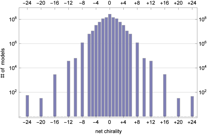
Figure 1: Number of models versus net chirality $N_{16}-N_{\overline{16}}$ in a random sample of $10^{9}$ $SO(10)$ models.

In addition, this method has been also successfully applied in the analysis of Pati–Salam and flipped $SU(5)$ vacua. However, a straightforward implementation in the case of standard model like vacua under consideration turns out to be practically impossible. The reason being that the phenomenologically acceptable models are too rare to be located using fully randomised search. Moreover, as will become clearer in the following, interesting SM vacua are not evenly spaced, but are concentrated in small regions of the parameter space, around specific fertile $SO(10)$ cores defined in Section 3.2.2. To demonstrate this we split the parameter space $\Pi$ in a product of two spaces $\Pi=\Pi_{1}\times{\Pi_{2}}$. The former $\Pi_{1}$ comprises GGSO phases that involve the first 12 basis vectors preserving the $SO(10)$ gauge symmetry whilst the latter $\Pi_{2}$ includes all GGSO phases related to the $SO(10)$ breaking vectors $\alpha,\beta$. Following Section 3.2.2, $\Pi_{1}$ includes 44 parameters given in (37), whereas $\Pi_{2}$ consists of the 18 parameters of (44).

Let us focus on the $\Pi_{1}$ subspace. It comprises $2^{44}\sim 2.\times 10^{13}$ $SO(10)$ configurations. We can apply a random sampling method to study their basic features. To this end we have generated a random sample of $10^{9}$ vacua and calculated the number of spinorial/antispinorial and vectorial representations for each model using equations (25), (26) and (30). This sampling is quite dense as it comprises approximately one in $10^{4}$ models of this subspace. The results for the number of models as a function of the net chirality $N_{16}-N_{\overline{16}}$ are depicted in Figure 1. We recover the usual bell shape distribution of $SO(10)$ vacua [14]. However, at this point one has to take into account an additional constraint. As explained in Section 3.2.2, when considering the $\beta$ related projections some spinorials are entirely projected out and do not give rise to offspring standard model states. However, these fertile spinorials can be traced back in the $\Pi_{1}$ parameter space. Thus, the effective net chirality is that of the fertile spinorials $N^{f}_{16}-N^{f}_{\overline{16}}$ as defined in (34), (35). We have performed a similar analysis in our random $SO(10)$ model sample and plotted the number of models versus the fertile net chirality in Figure 2.

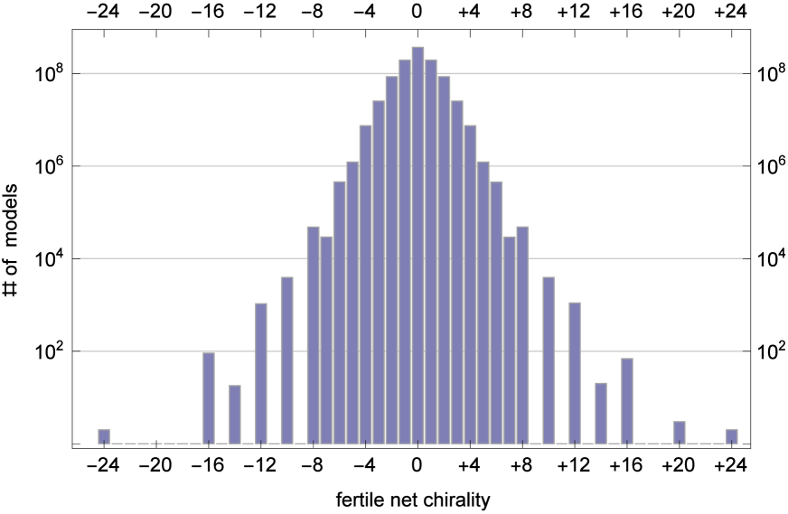
Figure 2: Number of models versus fertile net chirality $N^{f}_{16}-N^{f}_{\overline{16}}$ in a random sample of $10^{9}$ $SO(10)$ configurations.

Moreover, the final net chirality is also affected by the truncation of the SM states accommodated in spinorial representations due to the $\alpha,\beta$ projections. As can be seen from table 1 for fixed values of these projections each spinorial is split into four parts out of which only one survives. As a result we need at least $4\times 3=12$ generations at this level in order end up with three generations at the SM level. Consequently, only vacua with fertile net chirality 12 can give rise to three generation models after the application of the $SO(10)$ breaking projections. Another important phenomenological requirement is the existence of Higgs doublets in the low energy effective theory spectrum. At least one massless pair is needed in the minimal supersymmetric scenario. Appropriate Higgs doublets are accommodated into $SO(10)$ vectorials that arise both from the twisted and the untwisted sectors. However, it can be shown that in the class of models under consideration the $\alpha$ GGSO projections eliminate all untwisted doublets [36]. Hence, we have to look for the necessary SM Higgs doublets among the twisted sector $SO(10)$ vectorials. Using similar arguments, as in the case of spinorials, we conclude that the number of vectorials that satisfy the GGSO projections related to $\Pi_{1}$ and give rise to Higgs doublets is effectively reduced due to two reasons. First, some of them become inactive as they do not abide by the fertility condition (33). Second, as vectorials are also subject to truncation due to the $\alpha,\beta$ projections they can give rise to additional triplets instead of doublets. A look at table 2 is enough to convince us that we need at least two fertile vectorials at the $SO(10)$ level in order to produce the required Higgs doublet pair at the SM level. A plot of the number of models in our sample with $N_{16}-N_{\overline{16}}=12$ versus the number of $SO(10)$ vectorials is presented in Figure 3.

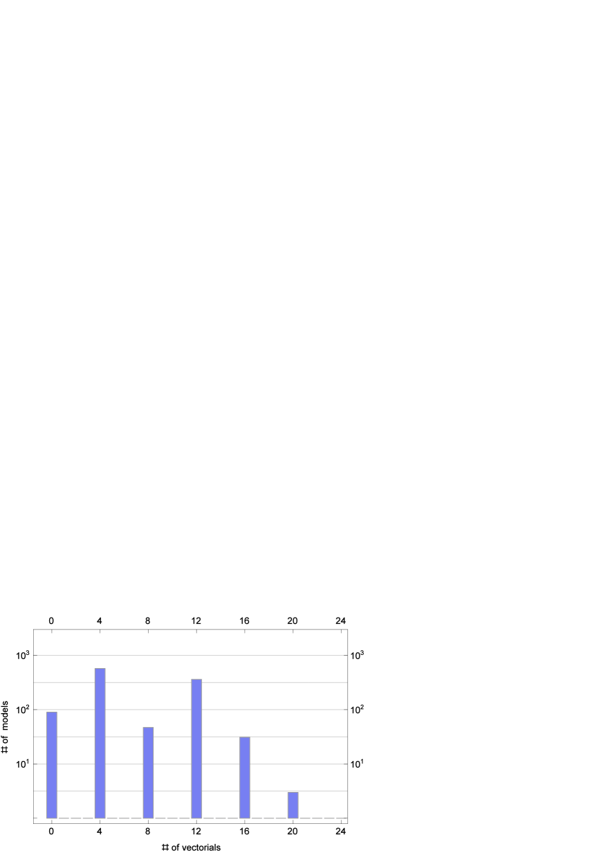
Figure 3: Number of models with fertile net chirality $N^{f}_{16}-N^{f}_{\overline{16}}=12$ versus number of twisted fertile vectorial representations in a random sample of $10^{9}$ $SO(10)$ vacua.

As seen from the figure a number of models, namely those with $N^{10}_{f}=0$, in Figure 3 fail to comply with this requirement and are thus excluded. Moreover, there are no models with $N^{f}_{10}=2$. Altogether, it turns out that approximately one in a million $SO(10)$ configurations in $\Pi_{1}$ give rise to phenomenologically acceptable offspring SM spectra.

Let us now turn to the $\Pi_{2}$ subspace. It contains 18 parameters thus it amounts to $2^{18}\sim 2.6\times 10^{5}$ distinct coefficient choices. A preliminary computer search shows that when combined with a legitimate $\Pi_{1}$ model they give rise to $2.2\times 10^{4}$ acceptable SM vacua on the average. That is one in ten configurations. Altogether the abundance of acceptable vacua is $2.2\times 10^{4}\times 10^{3}:2.6\times 10^{5}\times 10^{9}\sim 1:10^{7}$. Collecting a reasonable set of say $10^{6}$ SMs would require examining a sample of $10^{13}$ configurations. The problem becomes more difficult in practice as the distribution of acceptable vacua is not homogeneous. To resolve this issue we introduce a new search strategy consisting of a random scan in the parameter space $\Pi_{1}$ combined with a comprehensive scan of $\Pi_{2}$. More particularly, we first perform a random search in $\Pi_{1}$ for $SO(10)$ models that satisfy the aforementioned constraints

$$N^{f}_{16}-N^{f}_{\overline{16}}=12\ ,\ N^{f}_{10}\geq 2\$$ (61)

and collect the associated matching model data. Afterwords, for each of the assembled configurations we perform a comprehensive scan of the parameter space $\Pi_{2}$ and classify the resulting acceptable model spectra according to their main phenomenological properties. At this step, a model is considered as acceptable if it satisfies the minimal set of phenomenological criteria of Eqs. (46), (47), (48). This method turned out to be very efficient. A random scan of $10^{9}$ $SO(10)$ configurations in $\Pi_{1}$ took approximately 8 hours in a computer equipped with Intel i7 CPU (4 cores) running at 2.93GHz and 12 GB of RAM and produced 1011 matching $SO(10)$ models. Then a full scan of the $\Pi_{2}$ parameter space required around 5 additional hours and yielded approximately $2.2\times 10^{7}$ acceptable models. The main characteristics of these models together with their multiplicities are summarised in table 3. For each different model we list $n(Q),n(L),n(d^{c})=n(\nu^{c}),n(u^{c})=n(e^{c})$ i.e. the multiplicities of the associated standard model fields together with $n(\overline{Q}),n(\overline{L}),n(\overline{d^{c}})=n(\overline{\nu^{c}}),n(\overline{u^{c}})=n(\overline{e^{c}})$ the multiplicities of potential fields in conjugate representations arising from $SO(10)$ spinorials/antispinorials as well as the numbers of Higgs doublet pairs $n(H_{u})=n(H_{d})$ and additional triplet pairs $n({d^{c}}^{\prime})=n(\overline{{d^{c}}^{\prime}})$ arising from $SO(10)$ vectorials.

Some comments are in order here concerning the model multiplicity in table 3. First, a part of this degeneracy is due to permutation symmetry. More particularly, as the basis vectors $v_{1},\dots v_{14}$ treat the three orbifold planes symmetrically it is expected that for every model with a certain distribution of states in the three twisted planes, say $\left(\Xi_{1},\Xi_{2},\Xi_{3}\right)$ with $\Xi_{I}$ the subset of states in the I-the twisted plane, there exist equivalent models where two of the three subsets are interchanged e.g $\left(\Xi_{2},\Xi_{1},\Xi_{3}\right)$. We will explain below, in the discussion concerning the top quark Yukawa coupling how this degeneracy can be lifted. Second, in the computation of model multiplicity we have ignored all information regarding exotic/fractional charge states, hidden sector states etc. Thus, models considered as equivalent in table 3 could differ substantially with respect to the hidden sector and/or fractional/exotic state spectra. Third, even in the case where two models have identical spectra they could differ substantially at the level of interactions.

	$n(Q)$	$n(L)$	$n(d^{c})$ $n(\nu^{c})$	$n(u^{c})$ $n(e^{c})$	$n(\overline{Q})$	$n(\overline{L})$	$n(\overline{d^{c}})$ $n(\overline{\nu^{c}})$	$n(\overline{u^{c}})$ $n(\overline{e^{c}})$	$n(H_{u})$ $n(H_{d})$	$n({d^{c}}^{\prime})$ $n(\overline{{d^{c}}^{\prime}})$	Multiplicity
1	3	3	3	3	0	0	0	0	1	1	10748928
2	3	3	3	3	0	0	0	0	3	3	7635968
3	3	3	3	3	0	0	0	0	2	0	1697792
4	3	3	3	3	0	0	0	0	2	2	669696
5	3	3	3	3	0	0	0	0	1	5	298496
6	3	3	3	3	0	0	0	0	5	1	298496
7	4	4	4	4	1	1	1	1	1	1	49152
8	3	3	3	3	0	0	0	0	2	4	34816
9	3	3	3	3	0	0	0	0	4	2	34816
10	3	3	3	3	0	0	0	0	1	3	28672
11	3	3	3	3	0	0	0	0	3	1	28672
12	3	3	4	4	0	0	1	1	2	0	24576
13	4	4	3	3	1	1	0	0	2	0	24576
14	4	4	3	3	1	1	0	0	3	5	16640
15	3	3	4	4	0	0	1	1	5	3	16640
16	3	3	4	4	0	0	1	1	3	5	16640
17	4	4	3	3	1	1	0	0	5	3	16640
18	3	4	4	3	0	1	1	0	4	4	16384
19	4	3	3	4	1	0	0	1	4	4	16384
20	3	4	3	4	0	1	0	1	4	4	16384
21	4	3	4	3	1	0	1	0	4	4	16384
22	3	4	4	3	0	1	1	0	2	2	12288
23	4	3	3	4	1	0	0	1	2	2	12288
24	3	4	3	4	0	1	0	1	2	2	12288
25	4	3	4	3	1	0	1	0	2	2	12288
26	3	3	4	4	0	0	1	1	1	1	12288
27	4	4	3	3	1	1	0	0	1	1	12288
28	3	3	3	3	0	0	0	0	4	0	9216
29	4	4	4	4	1	1	1	1	2	0	8192
30	4	4	3	3	1	1	0	0	3	1	7680
31	3	3	4	4	0	0	1	1	3	1	7680
32	4	4	3	3	1	1	0	0	1	3	6144
33	3	3	4	4	0	0	1	1	1	3	6144
34	3	4	4	3	0	1	1	0	1	1	6144
35	4	3	3	4	1	0	0	1	1	1	6144
36	3	4	3	4	0	1	0	1	1	1	6144
37	4	3	4	3	1	0	1	0	1	1	6144
38	3	3	4	4	0	0	1	1	1	7	2816
39	4	4	3	3	1	1	0	0	7	1	2816
40	3	3	4	4	0	0	1	1	7	1	2816
41	4	4	3	3	1	1	0	0	1	7	2816
42	3	5	3	3	0	2	0	0	1	3	1536
43	5	3	3	3	2	0	0	0	1	3	1536
44	3	3	3	5	0	0	0	2	3	1	1536
45	3	3	5	3	0	0	2	0	3	1	1536
46	3	5	3	3	0	2	0	0	3	1	1536
47	5	3	3	3	2	0	0	0	3	1	1536
48	3	3	3	5	0	0	0	2	1	3	1536
49	3	3	5	3	0	0	2	0	1	3	1536

Table 3: Distinct standard like models with respect to the phenomenological characteristics under consideration and their multiplicities. The models are derived utilising a search over a random sample of $10^{9}$ configurations in the $SO(10)$ preserving parameter subspace $\Pi_{1}$ combined with a comprehensive scan in the $SO(10)$ breaking parameter subspace $\Pi_{2}$.

Another phenomenological characteristic of particular interest is the existence of a Yukawa coupling providing mass to the heaviest quark, namely the top quark. The conditions ensuring the presence of such coupling at the tri-level low energy effective superpotential have been derived in Section 4. They are expressed in terms of GGSO phase relations (55),(60). As a result, their implementation is straightforward, it suffices to match the standard like models derived above towards the criteria (55),(60). The results of this analysis are shown in table 3 where we list the main characteristics and multiplicities of distinct standard like models possessing a top quark Yukawa coupling. It turns out that almost half of the different models in table 3 are endowed with a top quark mass potential term. Caution must be taken in comparing the model multiplicities of tables 3 and 4. In the implementation of the top quark mass constraints we have made certain assumptions about the origin of the states involved ($Q^{3},{d^{c}}^{3},H_{u}$). Without loss of generality these assumptions lift some degeneracy of the spectra related to twisted plane permutation symmetries. Consequently, multiplicities in the last column of table 4 have to be raised by an extra factor when compared to those of the last column of table 3. This factor amounts e.g for assigning $Q^{3}$ state to $B^{1}_{0000}$ sector, ${u^{c}}^{3}$ to $B^{2}_{0000}$ etc.

	$n(Q)$	$n(L)$	$n(d^{c})$ $n(\nu^{c})$	$n(u^{c})$ $n(e^{c})$	$n(\overline{Q})$	$n(\overline{L})$	$n(\overline{d^{c}})$ $n(\overline{\nu^{c}})$	$n(\overline{u^{c}})$ $n(\overline{e^{c}})$	$n(H_{u})$ $n(H_{d})$	$n({d^{c}}^{\prime})$ $n(\overline{{d^{c}}^{\prime}})$	Multiplicity
1	3	3	3	3	0	0	0	0	1	1	27264
2	3	3	3	3	0	0	0	0	3	3	16896
3	3	3	3	3	0	0	0	0	2	0	7296
4	3	3	3	3	0	0	0	0	2	2	2304
5	3	3	3	3	0	0	0	0	5	1	1536
6	4	3	3	4	1	0	0	1	2	2	768
7	3	4	3	4	0	1	0	1	2	2	768
8	3	3	3	3	0	0	0	0	1	5	640
9	4	4	3	3	1	1	0	0	5	3	512
10	3	3	4	4	0	0	1	1	3	1	384
11	3	3	4	4	0	0	1	1	1	3	384
12	3	3	3	3	0	0	0	0	3	1	256
13	4	4	3	3	1	1	0	0	3	5	256
14	3	3	4	4	0	0	1	1	7	1	192
15	4	4	3	3	1	1	0	0	3	1	192
16	3	3	3	5	0	0	0	2	3	1	192
17	3	3	3	5	0	0	0	2	1	3	192
18	3	3	3	3	0	0	0	0	1	3	128
19	3	4	3	4	0	1	0	1	4	4	128
20	3	4	4	3	0	1	1	0	4	4	128
21	4	3	4	3	1	0	1	0	4	4	128
22	4	3	3	4	1	0	0	1	4	4	128
23	3	3	4	4	0	0	1	1	5	3	64
24	3	3	4	4	0	0	1	1	3	5	64
25	3	3	4	4	0	0	1	1	1	7	64

Table 4: Main phenomenological features and multiplicities of distinct standard–like models endowed with a top quark mass Yukawa coupling. The models are derived utilising a search over a random sample of $10^{9}$ configurations in the $SO(10)$ preserving parameter subspace $\Pi_{1}$ combined with a full scan in the $SO(10)$ breaking parameter subspace $\Pi_{2}$. Assumptions have been made with regard to the sectors producing the associated states (see text for details).

As seen from tables 3 three generation SLM vacua display a variety of spectra including : (a) Models without additional twisted triplets, as model no 3 in the table. Although, untwisted triplets are not projected out they usually become superheavy through coupling with untwisted sector singlets that acquire vevs. Hence, these models deserve further study in conjunction with the issue of proton decay. (b) Models with additional vector-like standard model states, including $Q-\bar{Q}$ pairs. The presence of these states could raise the SM coupling unification scale to energies close to the string scale. (c) Models with $\nu^{c}-\bar{\nu}^{c}$ pairs. These can play the role of heavy Higgs that break the additional abelian symmetries giving rise to the standard hyperchange $U(1)_{Y}$ symmetry. This is a new feature that leads to a new class of SLMs that have not been studied previously. Interestingly enough, all above classes of models appear also in table 4, that is they possess a candidate top quark mass Yukawa coupling. We will study an exemplary model displaying some of the above characteristics in the next section.

6 An Exemplary Model

In this section we use our computerised trawling algorithm to extract and discuss one specific model in some detail. The entire spectrum of the model is derived and presented. The string vacuum contains three chiral 16 of $SO(10)$ decomposed under the $SU(3)\times SU(2)\times U(1)^{2}$ subgroup, plus the heavy and light Higgs representations required for realistic symmetry breaking and fermion mass generation. Distinctly from previous free fermionic SLM constructions, the heavy Higgs states in this model are obtained from standard $SO(10)$ representations. The string derived model contains an additional pair of vector–like $Q$ and ${\bar{Q}}$ states that can be used to mitigate the GUT versus heterotic–string gauge coupling unification problem. The string model is generated by the set of basis vectors given in eqs. (3,4, 5), and by the set of GGSO phases given in eq. (62).

$$(v_{i}|v_{j})\ \ =\ \ \bordermatrix{&~{}1&S&e_{1}&e_{2}&e_{3}&e_{4}&e_{5}&e_{6}&b_{1}&b_{2}&z_{1}&z_{2}&\alpha&\beta\cr 1&~{}1&1&0&0&0&0&0&0&1&1&0&0&0&{1\over 2}\cr S&~{}1&1&1&1&1&1&1&1&1&1&1&1&1&1\cr e_{1}&~{}0&1&1&0&0&0&0&0&0&0&0&0&1&0\cr e_{2}&~{}0&1&0&1&1&0&0&0&1&0&0&0&0&0\cr e_{3}&~{}0&1&0&1&1&1&0&0&0&0&0&0&0&0\cr e_{4}&~{}0&1&0&0&1&1&0&0&0&0&1&0&0&0\cr e_{5}&~{}0&1&0&0&0&0&1&0&0&0&0&0&1&0\cr e_{6}&~{}0&1&0&0&0&0&0&1&0&0&0&0&0&1\cr b_{1}&~{}1&0&0&1&0&0&0&0&1&0&1&0&0&{1\over 2}\cr b_{2}&~{}1&0&0&0&0&0&0&0&0&1&0&0&0&-{1\over 2}~{}~{}\cr z_{1}&~{}0&1&0&0&0&1&0&0&1&0&0&1&0&{1\over 2}\cr z_{2}&~{}0&1&0&0&0&0&0&0&0&0&1&0&0&1\cr\alpha&~{}0&1&1&0&0&0&1&0&1&1&1&0&0&1\cr\beta&~{}1&1&0&0&0&0&0&1&0&1&0&0&0&{1\over 2}\cr}$$ (62)

where we used the notation $c{v_{i}\atopwithdelims[ ]v_{j}}=e^{i\pi(v_{i}|v_{j})}$. The spacetime vector bosons in the model are obtained from three sectors: the Neveu–Schwarz (NS) sector; the $z_{2}$–sector; and the $x+2\beta$–sector. The vector bosons from the NS–sector generate the observable and hidden sector symmetries given in eqs. (9) and (10). The $z_{2}$–sector enhances the $SU(2)_{h2}\times SU(2)_{h3}\times U(1)_{SU(4)_{h}}$ to an hidden $SU(4)_{h}$ gauge symmetry, whereas the vector boson states from the $z_{3}$–sector enhance the $SU(2)_{h1}\times SU(2)_{h4}$, together with the real fermion $\bar{\omega}_{2}$ to $SO(5)$. The $U(1)$ combinations are:

$$U(1)_{SU(4)} = U_{h4}+U_{h2}+U_{h3}~{},$$ (63)

$$U(1)_{5^{\prime}}~{}~{}~{}~{} = U_{h4}-U_{h2}-U_{h3}~{},$$ (64)

$$U(1)_{6^{\prime}}~{}~{}~{}~{} = ~{}~{}~{}~{}~{}~{}~{}~{}U_{h2}-U_{h3}~{}.$$ (65)

We emphasize that the non–simply laced $SO(5)$ symmetry is generated due to the fact that the states from the $z_{3}$–sector, that enhance the untwisted gauge symmetry, are obtained by acting on the vacuum with the real fermion oscillator $\bar{\omega}_{2}$. One generator in the Cartan sub–algebra is projected out and the roots are not charged under the associated broken $U(1)$ symmetry. Consequently, the roots obtained from the $z_{3}$–sector have length 1 and the resulting group is non–simply laced. Extensive investigations of using real fermions in similar constructions are discussed in ref. [38]. The full massless matter spectrum of the model is displayed in tables 5, 6, LABEL:tableslmexotics, LABEL:tablePSe, LABEL:tablefsu5e, LABEL:tableso10singlets. The model possess $N=1$ spacetime supersymmetry and therefore all the states shown in the table are in super–multiplets. Table 5 shows the untwisted matter states that are charged under the observable gauge group. A single untwisted state, $V_{33}$, which is charged under the hidden sector gauge group is shown in table LABEL:tableso10singlets. Table 6 shows the observable matter states. The states in table 6 are charged only under the observable gauge symmetry in eq. (9) but not under the hidden gauge symmetry in eq. (10). As seen from table 6 the model contains three chiral generations and the required heavy and light Higgs states for $U(1)_{Z^{\prime}}$ and electroweak symmetry breaking. The observable spectrum of this model exhibits several novel features compared to the earlier SLM free fermionic constructions [7]. The model contains the state ${\bar{N}}_{1}$, which together with a combination of the $N_{i},~{}i=1,\cdots,4$ can be used to break the $U(1)_{Z^{\prime}}$ symmetry along flat directions. This should be contrasted with the earlier SLM models in which such a state was absent. Those models therefore necessarily utilised exotic states that carry fractional $U(1)_{Z^{\prime}}$ charge. Breaking the $U(1)_{Z^{\prime}}$ gauge symmetry with states that carry standard GUT charges leaves a remnant local discrete symmetry [39] that protects the exotic states from decaying into the Standard Model states. In this case the exotic states provide viable dark matter candidates [28]. However, in the absence of states with standard GUT charges, exotically charged states are utilised [7], which does not leave a remnant discrete symmetry. The dark matter scenario of ref. [28] was recently realised in [40] with states that are exotic with respect to $E_{6}$, but are singlets under the $SO(10)$ gauge group, i.e. these states are neutral under the $U(1)_{Z^{\prime}}$ symmetry of eq. (12). The model presented here therefore provides examples of viable dark matter candidates that are Standard Model singlets and are charged under this $U(1)_{Z^{\prime}}$ combination. These states are shown in table LABEL:tableslmexotics. The second novel property of this model compared to the earlier construction of [7] is the additional pair of $Q$ and ${\bar{Q}}$, that may play a role in resolving the discrepancy between the GUT and heterotic string unification scales [41, 42].

The states displayed in table LABEL:tableso10singlets are singlets of $SO(10)$ and hence neutral under the Standard Model subgroup. They are charged with respect to the observable and hidden $U(1)$ gauge symmetries and may transform in non–Abelian representations of the hidden $SU(4)\times SO(5)$ gauge symmetry. The last state appearing in table LABEL:tableso10singlets, $V_{33}$, is obtained from the untwisted sector, whereas all other states are obtained from the twisted sectors. The untwisted state $V_{33}$ arises due to the gauge symmetry enhancement from the $z_{3}$–sector.

The states displayed in tables LABEL:tableslmexotics, LABEL:tablePSe and LABEL:tablefsu5e are exotic states that arise due to the Wilson line breaking of the $SO(10)$ GUT symmetry. As discussed in section 3.2.4 these states are classified according to the $SO(10)$ subgroup that is left unbroken in the sectors from which they arise. The states in tables LABEL:tablePSe and LABEL:tablefsu5e leave unbroken the $SO(6)\times SO(4)$ and $SU(5)\times U(1)$ subgroups, respectively, and therefore also arise in the free fermionic Pati–Salam [8, 15] and flipped $SU(5)$ [6, 41, 17, 18] type models. The states from these sectors carry fractional electric charge $\pm 1/2$, which are highly constrained by observations [27]. We note that a proposed resolution is that all the fractionally charged states transform in non–Ableian representations of the hidden sector gauge group and are confined into integrally charged states [43]. This is similar to the situation with the SLM exotics in table LABEL:tableslmexotics, which all transform under the hidden $SU(4)$ gauge symmetry. Indeed, that is also the case with the fractionally charged states appearing in table LABEL:tableslmexotics. However, while this is indeed the case in the flipped $SU(5)$ model of ref. [6], it does not in general hold in the space of flipped $SU(5)$ [17] or Pati–Salam heterotic–string vacua [15]. An alternative possibility is that the fractionally charged states obtain string scale mass from effective mass terms in the superpotential [26]. The most compelling possibility, however, is that fractionally charged states appear as massive states in the string spectrum, but not at the massless level. Indeed, such Pati–Salam models were found in ref. [15, 16, 24] and were dubbed exophobic string vacua. As seen from tables LABEL:tablePSe and LABEL:tablefsu5e the present model contains a variety of fractionally charged states.

sector	field	$SU(3)\times{SU(2)}_{L}\times{U(1)}_{C}\times U(1)_{L}$	${U(1)}_{1}$	${U(1)}_{2}$	${U(1)}_{3}$
$S$	$D_{1}$	$(3,\hphantom{+}1,{-1},\hphantom{+}0)$	$+1$	$\hphantom{+}0$	$\hphantom{+}0$
	$D_{2}$	$(3,\hphantom{+}1,{-1},\hphantom{+}0)$	$\hphantom{+}0$	$+1$	$\hphantom{+}0$
	$D_{3}$	$(3,\hphantom{+}1,{-1},\hphantom{+}0)$	$\hphantom{+}0$	$\hphantom{+}0$	$+1$
	$\bar{D}_{1}$	$({\bar{3}},\hphantom{+}1,+1,\hphantom{+}0)$	$-1$	$\hphantom{+}0$	$\hphantom{+}0$
	$\bar{D}_{2}$	$({\bar{3}},\hphantom{+}1,{+1},\hphantom{+}0)$	$\hphantom{+}0$	$-1$	$\hphantom{+}0$
	$\bar{D}_{3}$	$({\bar{3}},\hphantom{+}1,{+1},\hphantom{+}0)$	$\hphantom{+}0$	$\hphantom{+}0$	$-1$
	$\Phi_{12}$	$(1,\hphantom{+}1,\hphantom{+}0,\hphantom{+}0)$	$+1$	$-1$	$\hphantom{+}0$
	$\bar{\Phi}_{12}$	$(1,\hphantom{+}1,\hphantom{+}0,\hphantom{+}0)$	$-1$	$+1$	$\hphantom{+}0$
	$\Phi_{13}$	$(1,\hphantom{+}1,\hphantom{+}0,\hphantom{+}0)$	$+1$	$\hphantom{+}0$	$-1$
	$\bar{\Phi}_{13}$	$(1,\hphantom{+}1,\hphantom{+}0,\hphantom{+}0)$	$-1$	$\hphantom{+}0$	$+1$
	$\Phi_{23}$	$(1,\hphantom{+}1,\hphantom{+}0,\hphantom{+}0)$	$\hphantom{+}0$	$-1$	$+1$
	$\bar{\Phi}_{23}$	$(1,\hphantom{+}1,\hphantom{+}0,\hphantom{+}0)$	$\hphantom{+}0$	$+1$	$-1$
	$\Phi_{i},i=1,\dots,5$	$(1,\hphantom{+}1,\hphantom{+}0,\hphantom{+}0)$	$\hphantom{+}0$	$\hphantom{+}0$	$\hphantom{+}0$

Table 5: Observable untwisted matter spectrum and $SU(3)_{C}\times{SU(2)}_{L}\times{U(1)}_{C}\times U(1)_{L}\times{U(1)}^{3}$ quantum numbers.

sector	field	$SU(3)\times{SU(2)}_{L}\times{U(1)}_{C}\times U(1)_{L}$	${U(1)}_{1}$	${U(1)}_{2}$	${U(1)}_{3}$
$S+b_{1}+e_{3}+e_{4}+e_{6}$	${U}_{1}$	$({\bar{3}},\hphantom{+}1,-{1/2},-1)$	$-{1/2}$	$\hphantom{+}0$	$\hphantom{+}0$
	${E}_{1}$	$(1,\hphantom{+}1,{\hphantom{+}{3}/{2}},+1)$	$-{1/2}$	$\hphantom{+}0$	$\hphantom{+}0$
$S+b_{1}+e_{3}+e_{4}$	${D}_{1}$	$({\bar{3}},\hphantom{+}1,{-{1/2}},+1)$	$-{1/2}$	$\hphantom{+}0$	$\hphantom{+}0$
	${N}_{1}$	$(1,\hphantom{+}1,{\hphantom{+}{3/2}},-1)$	$-{1/2}$	$\hphantom{+}0$	$\hphantom{+}0$
$S+b_{1}+e_{3}+e_{4}+e_{5}+e_{6}$	$L_{1}$	$(1,\hphantom{+}2,{-{3/2}},\hphantom{+}0)$	$-{1/2}$	$\hphantom{+}0$	$\hphantom{+}0$
$S+b_{1}+e_{3}+e_{4}+e_{5}$	$Q_{1}$	$(3,\hphantom{+}2,{\hphantom{+}{1/2}},\hphantom{+}0)$	$-{1/2}$	$\hphantom{+}0$	$\hphantom{+}0$
$S+b_{2}+e_{1}+e_{5}$	${U}_{2}$	$({\bar{3}},\hphantom{+}1,{-{1/2}},-1)$	$\hphantom{+}0$	$-{1/2}$	$\hphantom{+}0$
	${E}_{2}$	$(1,\hphantom{+}1,{\hphantom{+}{3/2}},+1)$	$\hphantom{+}0$	$-{1/2}$	$\hphantom{+}0$
$S+b_{2}+e_{1}+e_{5}+e_{6}$	${D}_{2}$	$({\bar{3}},\hphantom{+}1,{-{1/2}},+1)$	$\hphantom{+}0$	$-{1/2}$	$\hphantom{+}0$
	${N}_{2}$	$(1,\hphantom{+}1,{\hphantom{+}{3/2}},-1)$	$\hphantom{+}0$	$-{1/2}$	$\hphantom{+}0$
$S+b_{2}+e_{1}$	$L_{2}$	$(1,\hphantom{+}2,{-{3/2}},\hphantom{+}0)$	$\hphantom{+}0$	$-{1/2}$	$\hphantom{+}0$
$S+b_{2}+e_{1}+e_{6}$	$Q_{2}$	$(3,\hphantom{+}2,{\hphantom{+}{1/2}},\hphantom{+}0)$	$\hphantom{+}0$	$-{1/2}$	$\hphantom{+}0$
$S+b_{2}+e_{1}+e_{5}$	${U}_{3}$	$({\bar{3}},\hphantom{+}1,{-{1/2}},-1)$	$\hphantom{+}0$	$-{1/2}$	$\hphantom{+}0$
	${E}_{3}$	$(1,\hphantom{+}1,{\hphantom{+}{3/2}},+1)$	$\hphantom{+}0$	$-{1/2}$	$\hphantom{+}0$
$S+b_{2}+e_{1}+e_{5}+e_{6}$	${D}_{3}$	$({\bar{3}},\hphantom{+}1,{-{1/2}},+1)$	$\hphantom{+}0$	$-{1/2}$	$\hphantom{+}0$
	${N}_{3}$	$(1,\hphantom{+}1,{\hphantom{+}{3/2}},-1)$	$\hphantom{+}0$	$-{1/2}$	$\hphantom{+}0$
$S+b_{2}+e_{1}$	$L_{3}$	$(1,\hphantom{+}2,{-{3/2}},\hphantom{+}0)$	$\hphantom{+}0$	$-{1/2}$	$\hphantom{+}0$
$S+b_{2}+e_{1}+e_{6}$	$Q_{3}$	$(3,\hphantom{+}2,{\hphantom{+}{1/2}},\hphantom{+}0)$	$\hphantom{+}0$	$-{1/2}$	$\hphantom{+}0$
$S+b_{3}+e_{1}$	${D}_{4}$	$({\bar{3}},\hphantom{+}1,{-{1/2}},\hphantom{+}1)$	$\hphantom{+}0$	$\hphantom{+}0$	$-{1/2}$
$S+b_{3}+e_{1}$	${N}_{4}$	$(1,\hphantom{+}1,{\hphantom{+}{3/2}},-1)$	$\hphantom{+}0$	$\hphantom{+}0$	$-{1/2}$
$S+b_{3}$	$Q_{4}$	$(3,\hphantom{+}2,{\hphantom{+}{1/2}},\hphantom{+}0)$	$\hphantom{+}0$	$\hphantom{+}0$	$-{1/2}$
$S+b_{3}+e_{1}+e_{3}$	${\bar{D}}_{1}$	$({3},\hphantom{+}1,\hphantom{+}{1/2},-1)$	$\hphantom{+}0$	$\hphantom{+}0$	$\hphantom{+}{1/2}$
$S+b_{3}+e_{1}+e_{3}$	${\bar{N}}_{1}$	$(1,\hphantom{+}1,{-{3}/{2}},+1)$	$\hphantom{+}0$	$\hphantom{+}0$	$\hphantom{+}{1/2}$
$S+b_{3}+e_{3}$	${\bar{Q}}_{1}$	$({\bar{3}},\hphantom{+}2,{-{1/2}},\hphantom{+}0)$	$\hphantom{+}0$	$\hphantom{+}0$	$\hphantom{+}{1/2}$
$S+b_{3}+x+e_{4}$	${\cal D}_{1}$	$({3},\hphantom{+}1,~{}~{}{-1},\hphantom{+}0)$	$-{1/2}$	$-{1/2}$	$\hphantom{+}0$
$S+b_{3}+x+e_{4}$	$S_{1}$	$({1},\hphantom{+}1,~{}~{}\hphantom{+}0,\hphantom{+}0)$	$\hphantom{+}{1/2}$	$\hphantom{+}{1/2}$	$+1$
$S+b_{3}+x+e_{3}+e_{4}$	${\bar{\cal D}}_{1}$	$({\bar{3}},\hphantom{+}1,~{}~{}{+1},\hphantom{+}0)$	$\hphantom{+}{1/2}$	$\hphantom{+}{1/2}$	$\hphantom{+}0$
$S+b_{3}+x+e_{3}+e_{4}$	${\bar{S}}_{1}$	$({1},\hphantom{+}1,~{}~{}\hphantom{+}0,\hphantom{+}0)$	$-{1/2}$	$-{1/2}$	$-1$
$S+b_{3}+x+e_{1}+e_{4}$	${h}_{1}$	$({1},\hphantom{+}2,~{}~{}\hphantom{+}0,-1)$	$\hphantom{+}{1/2}$	$\hphantom{+}{1/2}$	$\hphantom{+}0$
$S+b_{3}+x+e_{3}+e_{4}$	${\bar{h}}_{1}$	$({1},\hphantom{+}2,~{}~{}\hphantom{+}0,+1)$	$\hphantom{+}{1/2}$	$\hphantom{+}{1/2}$	$\hphantom{+}0$
$S+b_{1}+x+e_{3}+e_{5}+e_{6}$	$\zeta_{1}$	$({1},\hphantom{+}1,~{}~{}\hphantom{+}0,\hphantom{+}0)$	$\hphantom{+}0$	$\hphantom{+}{1/2}$	$-{1/2}$
$S+b_{1}+x+e_{5}+e_{6}$	${\cal D}_{2}$	$({1},\hphantom{+}1,~{}~{}-1,\hphantom{+}0)$	$\hphantom{+}0$	$\hphantom{+}{1/2}$	$\hphantom{+}{1/2}$
$S+b_{1}+x+e_{5}+e_{6}$	$\zeta_{a},~{}a=2,3$	$({1},\hphantom{+}1,~{}~{}~{}\hphantom{+}0,\hphantom{+}0)$	$\hphantom{+}0$	$\hphantom{+}{1/2}$	$-{1/2}$
$S+b_{1}+x+e_{5}+e_{6}$	${\bar{\zeta}}_{a},~{}a=2,3$	$({1},\hphantom{+}1,~{}~{}~{}\hphantom{+}0,\hphantom{+}0)$	$\hphantom{+}0$	$-{1/2}$	$\hphantom{+}{1/2}$
$S+b_{1}+x+e_{5}+e_{6}$	$\phi_{1}$	$({1},\hphantom{+}1,~{}~{}~{}\hphantom{+}0,\hphantom{+}0)$	$+1$	$-{1/2}$	$-{1/2}$
$S+b_{1}+x+e_{5}$	${\bar{\cal D}}_{2}$	$({1},\hphantom{+}1,~{}~{}+1,\hphantom{+}0)$	$\hphantom{+}0$	$\hphantom{+}{1/2}$	$\hphantom{+}{1/2}$
$S+b_{1}+x+e_{5}$	${\bar{S}}_{2}$	$({1},\hphantom{+}1,~{}~{}+1,\hphantom{+}0)$	$-1$	$-{1/2}$	$-{1/2}$
$S+b_{1}+x+e_{6}$	${h}_{2}$	$({1},\hphantom{+}2,~{}~{}\hphantom{+}0,-1)$	$\hphantom{+}0$	$\hphantom{+}{1/2}$	$\hphantom{+}{1/2}$
$S+b_{1}+x$	${\bar{h}}_{2}$	$({1},\hphantom{+}2,~{}~{}\hphantom{+}0,+1)$	$\hphantom{+}0$	$\hphantom{+}{1/2}$	$\hphantom{+}{1/2}$

Table 6: Twisted matter spectrum (observable sector) and $SU(3)_{C}\times{SU(2)}_{L}\times{U(1)}_{C}\times U(1)_{L}\times{U(1)}^{3}$ quantum numbers.

7 Conclusions

In this paper we extended the free fermionic classifications methodology to the class of Standard–like Models, in which the $SO(10)$ GUT symmetry is broken at the string level to $SU(3)\times SU(2)\times U(1)^{2}$. The SLM free fermionic heterotic–string models uniquely require two basis vectors that break the $SO(10)$ symmetry. One to the PS subgroup and one to the FSU5 subgroup. Compared to the PS and FSU5 cases this substantially increases the computational complexity of the analysis of the SLM vacua. Compared to the classifications of the corresponding PS and FSU5 models, the space of SLM models is vastly increased. To extract the phenomenologically interesting three generation models therefore required adaptation of the methodology. Rather than generating random phases of the entire space of vacua, we divided the process in two steps. The first involves imposing a set of constraints on the GGSO phases of models with $SO(10)$ GUT symmetry. These constraints pre–select $SO(10)$ GGSO configurations that yield three generation models, and are dubbed as fertile $SO(10)$ models. At this level we generate random choices of GGSO configurations that satisfy the fertility constraints. To these preselected configurations we add the $SO(10)$ breaking basis vectors, and perform a complete classification of the additional GGSO coefficients, resulting in some $10^{7}$ three generation Standard–like Models. Additionally, we discussed the imposition of a viable top quark Yukawa couplings in the selection process, and the reduction of model degeneracy, which is obtained by fixing the $Z_{2}\times Z_{2}$ orbifold planes from which the top quark left and right components are obtained. We further used our computerised method to explore in detail an exemplary three generation SLM model with special phenomenological properties, which were not obtained in previous SLM constructions. The first is the presence of an additional pair of right–handed neutrino and its conjugated field. These can be used as heavy Higgs representations to break the additional $U(1)_{Z^{\prime}}$ of eq. (12) along supersymmetric flat directions, whereas in earlier models exotic states with fractional $U(1)_{Z^{\prime}}$ charge were used for that purpose [7]. The consequence is that in our new model one can realise the dark matter scenario discussed in ref. [28], whereas this was not possible in the models of refs. [7]. The second distinct property of our new model is the existence of an additional pair of $Q$, ${\bar{Q}}$ states that may be instrumental in mitigating the heterotic–string gauge coupling unification problem [41, 42].

The methodology developed in this work therefore enables us to generate a larger number of phenomenologically viable SLM free fermionic heterotic–string vacua, as compared to the earlier trial–and–error method of [7]. One can envision using this method to delve deeper in the phenomenological detail. In this paper we focused on the analysis of the observable Standard Model matter states. Analysis of the enhanced symmetries and exotic states can be further developed, along the lines of earlier classifications [15, 17, 18, 44]. Furthermore, the vast space of GGSO configurations entailed that our analysis here is slated toward models that can produce phenomenologically viable models. It would therefore be of interest to develop alternative computerised methods, such as those developed in refs. [45], and to explore the symmetries underlying the larger space of vacua.

References

- [1] P. Candelas, G.T. Horowitz, A. Strominger and E. Witten, Nucl. Phys. B258 (1985) 46.
- [2] D.J. Gross, J.A. Harvey, E.J. Martinec and R. Rohm, Nucl. Phys. B267 (1986) 75.
- [3] For review and references see e.g: L.E Ibanez and A.M Uranga, String theory and particle physics: an introduction to string phenomenology, Cambrdige University Press, 2012.
-
[4]
I. Antoniadis, C. Bachas, and C. Kounnas, Nucl. Phys. B289 (1987) 87;
H. Kawai, D.C. Lewellen, and S.H.-H. Tye, Nucl. Phys. B288 (1987) 1;
I. Antoniadis and C. Bachas, Nucl. Phys. B298 (1988) 586. -
[5]
A.E. Faraggi, Phys. Lett. B326 (1994) 62; Phys. Lett. B544 (2002) 207;
E. Kiritsis and C. Kounnas, Nucl. Phys. B503 (1997) 117;
A.E. Faraggi, S. Forste and C. Timirgaziu, JHEP 0608 (2006) 057;
P. Athanasopoulos, A.E. Faraggi, S. Groot Nibbelink and V.M. Mehta, JHEP 1604 (2016) 038. - [6] I. Antoniadis, J. Ellis, J. Hagelin and D.V. Nanopoulos, Phys. Lett. B231 (1989) 65
-
[7]
A.E. Faraggi, D.V. Nanopoulos and K. Yuan,
Nucl. Phys. B335 (1990) 347;
A.E. Faraggi, Phys. Lett. B278 (1992) 131; Nucl. Phys. B387 (1992) 239;
G.B. Cleaver, A.E. Faraggi and D.V. Nanopoulos, Phys. Lett. B455 (1999) 135;
A.E. Faraggi, E. Manno and C.M. Timirgaziu, Eur. Phys. Jour. C50 (2007) 701. -
[8]
I. Antoniadis. G.K. Leontaris and J. Rizos,
Phys. Lett. B245 (1990) 161;
G.K. Leontaris and J. Rizos, Nucl. Phys. B554 (1999) 3. - [9] G.B. Cleaver, A.E. Faraggi and C. Savage, Phys. Rev. D63 (2001) 066001; G.B. Cleaver, D.J Clements and A.E. Faraggi, Phys. Rev. D65 (2002) 106003;
-
[10]
G.B. Cleaver, A.E. Faraggi and S.E.M. Nooij,
Nucl. Phys. B672 (2003) 64;
A.E. Faraggi and H. Sonmez, Phys. Rev. D91 (2015) 066006. - [11] A.E. Faraggi and D.V. Nanopoulos, Phys. Rev. D48 (1993) 3288.
- [12] A. Gregori, C. Kounnas and J. Rizos, Nucl. Phys. B549 (1999) 16.
- [13] A.E. Faraggi, C. Kounnas, S.E.M. Nooij and J. Rizos, hep-th/0311058; Nucl. Phys. B695 (2004) 41.
- [14] A.E. Faraggi, C. Kounnas and J. Rizos, Phys. Lett. B648 (2007) 84; Nucl. Phys. B774 (2007) 208; Nucl. Phys. B799 (2008) 19.
-
[15]
B. Assel, C. Christodoulides, A.E. Faraggi, C. Kounnas and J. Rizos
Phys. Lett. B683 (2010) 306; Nucl. Phys. B844 (2011) 365;
C. Christodoulides, A.E. Faraggi and J. Rizos, Phys. Lett. B702 (2011) 81. - [16] L. Bernard et al, Nucl. Phys. B868 (2013) 1.
- [17] A.E. Faraggi, J. Rizos and H. Sonmez, Nucl. Phys. B886 (2014) 202.
- [18] H. Sonmez, Phys. Rev. D93 (2016) 125002.
-
[19]
See e.g.: D. Senechal, Phys. Rev. D39 (1989) 3717;
K.R. Dienes, Phys. Rev. Lett. 65 (1990) 1979; Phys. Rev. D73 (2006) 106010;
M.R. Douglas, JHEP 0305 (2003) 046;
R. Blumenhagen et al, Nucl. Phys. B713 (2005) 83;
F. Denef and M.R. Douglas, JHEP 0405 (2004) 072;
T.P.T. Dijkstra, L. Huiszoon and A.N. Schellekens, Nucl. Phys. B710 (2005) 3;
B.S. Acharya, F. Denef and R. Valadro, JHEP 0506 (2005) 056;
P. Anastasopoulos, T.P.T. Dijkstra, E. Kiritsis and A.N. Schellekens, Nucl. Phys. B759 (2006) 83;
M.R. Douglas and W. Taylor, JHEP 0701 (2007) 031;
K.R. Dienes, M. Lennek, D. Senechal and V. Wasnik, Phys. Rev. D75 (2007) 126005;
O. Lebedev et al, Phys. Lett. B645 (2007) 88;
E. Kiritsis, M. Lennek and A.N. Schellekens JHEP 0902 (2009) 030;
L.B. Anderson, A. Constantin, J. Gray, A. Lukas and E. Palti, JHEP 1401 (2014) 047. -
[20]
B.R. Greene and M.R. Plesser, Nucl. Phys. B338 (1990) 15;
P. Candelas, M. Lynker and R. Schimmrigk, Nucl. Phys. B341 (1990) 383. -
[21]
T. Catelin-Julian, A.E. Faraggi, C. Kounnas and J. Rizos,
Nucl. Phys. B812 (2009) 103;
C. Angelantonj, A.E. Faraggi and M. Tsulaia, JHEP 1007 (2010) 314;
A.E. Faraggi, I. Florakis, T. Mohaupt and M. Tsulaia, Nucl. Phys. B848 (2011) 332. - [22] P. Athanasoupoulos, A.E. Faraggi and D. Gepner, Phys. Lett. B735 (2014) 357.
- [23] P. Athanasopoulos and A.E. Faraggi, Adv. Math. Phys. 2017 (2017) 3572469.
- [24] A.E. Faraggi and J. Rizos, Nucl. Phys. B895 (2015) 233.
-
[25]
A.E. Faraggi and J. Rizos, Eur. Phys. Jour. C76 (2016) 170;
J. Ashfaque, L. Delle Rose, A.E. Faraggi and C. Marzo, Eur. Phys. Jour. C76 (2016) 570. - [26] A.E. Faraggi, Phys. Rev. D46 (1992) 3204.
- [27] See e.g. V. Halyo et al, Phys. Rev. Lett. 84 (2000) 2576.
-
[28]
S. Chang, C. Coriano and A.E. Faraggi, Nucl. Phys. B477 (1996) 65;
C. Coriano, A.E. Faraggi and M. Plümacher, Nucl. Phys. B614 (2001) 233. -
[29]
A.E. Faraggi and E. Halyo, Phys. Lett. B307 (1993) 416;
A.E. Faraggi and J. Pati, Phys. Lett. B400 (1998) 21;
C. Coriano and A.E. Faraggi, Phys. Lett. B581 (2004) 99. -
[30]
K.R. Dienes, Phys. Rev. Lett. 65 (1990) 1979; Phys. Rev. D42 (1990) 2004;
S. Abel and K.R. Dienes, Phys. Rev. D91 (2015) 126014;
J.M. Ashfaque, P. Athanasopoulos, A.E. Faraggi and H.Sonmez, Eur. Phys. Jour. C76 (2016) 208;
M. Blaszczyk, S. Groot Nibbelink, O. Loukas and F. Ruehle, JHEP 1510 (2015) 166;
S. Groot Nibbelink and E. Parr, Phys. Rev. D94 (2016) 041704;
I. Florakis and J. Rizos, Nucl. Phys. B913 (2016) 495;
I. Florakis, arXiv:1611.10323;
B. Aaronson, S. Abel and E. Mavroudi, arXiv:1612.05742. - [31] see e.g.: S. Raby, Lect. Notes. Phys. 939 (2017) 1, and references therein.
- [32] T. Asaka, W. Buchmüller and L. Covi, Phys. Lett. B523 (2001) 199.
-
[33]
A.E. Faraggi, Nucl. Phys. B407 (1993) 57; Eur. Phys. Jour. C49 (2007) 803;
G. Cleaver and A.E. Faraggi, Int. J. Mod. Phys. A14 (1999) 2335. - [34] A.E. Faraggi, Nucl. Phys. B728 (2005) 83.
- [35] J. Rizos, Eur. Phys. Jour. C74 (2014) 2905.
- [36] A.E. Faraggi, Nucl. Phys. B428 (1994) 111; Phys. Lett. B520 (2001) 337.
- [37] A.E. Faraggi, Phys. Lett. B274 (1992) 47; Phys. Rev. D47 (1993) 5021.
-
[38]
D.C. Lewellen, Nucl. Phys. B337 (1990) 49;
K.R. Dienes and J. March–Russell, Nucl. Phys. B479 (1996) 113. - [39] A.E. Faraggi, Phys. Lett. B398 (1997) 88.
- [40] L. Delle Rose, A.E. Faraggi, C. Marzo and J. Rizos, Phys. Rev. D96 (2017) 055025, arXiv:1704.02579.
- [41] J.L Lopez, D.V. Nanopoulos and K. Yuan, Nucl. Phys. B399 (1993) 654.
-
[42]
A.E. Faraggi, Phys. Lett. B302 (1993) 202;
K.R. Dienes and A.E. Faraggi, Phys. Rev. Lett. 75 (1995) 2646; Nucl. Phys. B457 (1995) 409. -
[43]
J. Ellis, J.L. Lopez and D.V. Nanopoulos, Phys. Lett. B247 (1990) 257;
K. Benakli, J. Ellis and D.V. Nanopoulos, Phys. Rev. D59 (1999) 047301. - [44] H. Sonmez, University of Liverpool PhD thesis, 2015.
-
[45]
S. Abel and J. Rizos, JHEP 1408 (2014) 10;
R. Hogan, M. Fairbairn and N. Seeburn, Mon. Not. Roy. Astron. Soc. 449 (2015) 2040;
J.K. Behr et al, Eur. Phys. Jour. C76 (2016) 386;
F. Ruehle, JHEP 1708 (2017) 38;
J. Liu, arXiv:1707.02800;
J. Carifio, J. Halverson, D. Krioukov and B.D. Nelson, arXiv:1707.00655.