Inspiraling Halo Accretion Mapped in Lyman-$\alpha$ Emission around a $z\sim 3$ Quasar

Abstract

In an effort to search for Ly$\alpha$ emission from circum- and intergalactic gas on scales of hundreds of kpc around $z\sim 3$ quasar, and thus characterise the physical properties of the gas in emission, we have initiated an extensive fast-survey with the Multi Unit Spectroscopic Explorer (MUSE): Quasar Snapshot Observations with MUse: Search for Extended Ultraviolet eMission (QSO MUSEUM). In this work, we report the discovery of an enormous Ly$\alpha$ nebula (ELAN) around the quasar SDSS J102009.99+104002.7 at $z=3.164$, which we followed-up with deeper MUSE observations. This ELAN spans $\sim 297$ projected kpc, has an average Ly$\alpha$ surface brightness ${\rm SB}_{\rm Ly\alpha}\sim 6.04\times 10^{-18}$erg s^-1 cm^-2 arcsec^-2(within the $2\sigma$ isophote), and is associated with an additional four, previously unknown embedded sources: two Ly$\alpha$ emitters and two faint active galactic nuclei (one Type-1 and one Type-2 quasar). By mapping at high significance the line-of-sight velocity in the entirety of the observed structure, we unveiled a large-scale coherent rotation-like pattern spanning $\sim 300$ km s^-1 with a velocity dispersion of $<270$ km s^-1, which we interpret as a signature of the inspiraling accretion of substructures within the quasar’s host halo. Future multiwavelength data will complement our MUSE observations, and are definitely needed to fully characterise such a complex system. None the less, our observations reveal the potential of new sensitive integral-field spectrographs to characterise the dynamical state of diffuse gas on large scales in the young Universe, and thereby witness the assembly of galaxies.

1 Introduction

It is predicted that the universe’s initial conditions have zero net angular momentum. Yet spin is a fundamental property of galaxies, especially in disky spirals like our Milky Way. The accepted model of galaxy formation explains the required angular momentum build-up as follows. During the Universe’s lifespan, baryons collapse into the potential well of dark matter (DM) haloes from the “cosmic web”, i.e. the diffuse intergalactic medium (IGM) tracing the large-scale structure in the universe. In this process, the gas is shock-heated to the virial temperature of the DM haloes, and subsequently cools down and settles in galaxies, where it is partially transformed into stars (White & Rees 1978). In the initial phases of the collapse, the gravitational forces exerted between neighbouring DM haloes produce torques which generate a net angular momentum within these systems (Hoyle 1951). In an expanding universe (Hubble 1929), this initial phase of angular momentum build-up ends when the DM haloes become bound structures in themselves, sufficiently far away from their neighbours such that the large scale gravitational torques stop being the dominant evolutionary force. As a result, the angular momentum acquired at earlier epochs forces the baryons to assemble in rotating structures inside haloes (Fall & Efstathiou 1980). Following this theory, analytic calculations predicted spins for modern galaxies (Peebles 1969), which have been confirmed by numerical simulations within our modern cosmological paradigm (e.g. Bullock et al. 2001; Porciani et al. 2002).

In the past decade, an important element has been added to this picture. Hydrodynamic simulations of galaxy formation have started to show the accretion of “streams” of cool gas into dark matter haloes (Kereš et al. 2005). These streams are predicted to fuel star-formation within the central galaxy (Dekel & Birnboim 2006), funnel dwarf galaxies into the surrounding dark matter halo, and provide a reservoir of cool halo gas (Faucher-Giguère & Kereš 2011; Fumagalli et al. 2011). Recent numerical work has found that the baryons within these streams exhibit a significantly higher angular momentum than the matter within the inner regions of the dark matter haloes. This suggests that streams contribute to the net angular momentum of the system (Stewart et al. 2011; Danovich et al. 2015). These same models predict that large regions of the halo may contain inspiraling gas or structures with a projected velocity shear qualitatively similar to rotation (Stewart et al. 2016). Therefore, both these channels of accretion available to baryons would lead to the presence of cool gaseous structures within galaxy haloes carrying a net angular momentum.

Unfortunately, the halo gas, i.e. the so-called circumgalactic medium (CGM), is expected to have very low densities, and thus to be typically too faint to detect directly. Observations using the light from bright background sources to probe haloes along individual sightlines have revealed a high covering fraction of cool gas around high-$z$ galaxies (Rudie et al. 2012; Prochaska et al. 2013a; Prochaska et al. 2013b, 2014). This cool CGM is manifest around galaxies of essentially all luminosity and mass, and across all of cosmic time (e.g., Prochaska et al. 2011; Tumlinson et al. 2013). The absorption-line experiment, however, cannot resolve the ‘morphology’ of the CGM, and given that it is an inherently one-dimensional probe, it does not uniquely constrain kinematics relevant to the angular momentum of the system. The past few years, however, have witnessed the discovery of enormous Ly$\alpha$ nebulae (ELANe) – cool, emitting hydrogen gas that extends hundreds of kpc around $z>2$ quasars (Cantalupo et al. 2014; Hennawi et al. 2015; Cai et al. 2017). On these scales, the Ly$\alpha$ emission probes gas throughout the dark matter halo and even beyond into the surrounding IGM. Furthermore, the emission is sufficiently bright (Ly$\alpha$ surface brightness ${\rm SB}_{\rm Ly\alpha}\sim 10^{-17}{\rm\,erg\,s^{-1}\,cm^{-2}\,arcsec^{-2}}$ at 100 kpc from the AGN) to measure line-of-sight velocities throughout the ELAN. In turn, one may search for signatures of inspiraling gas predicted by models of galaxy formation.

However, ELANe seems to be extremely rare, and one would need a statistical sample to find such bright and thus “easy-to-observe” systems. Indeed, the reminder of the studies in the literature show (i) fainter Ly$\alpha$ emission at these large projected distances (100 kpc), ${\rm SB}_{\rm Ly\alpha}\sim 10^{-18}$erg s^-1 cm^-2 arcsec^-2 (Borisova et al. 2016; Fumagalli et al. 2016), (ii) detections only on smaller scales ($R<50$ kpc) in 50-70% of the cases (Hu & Cowie 1987; Heckman et al. 1991a, b; Christensen et al. 2006; North et al. 2012; Hennawi & Prochaska 2013; Roche et al. 2014; Arrigoni Battaia et al. 2016), or (iii) non-detections (e.g., Herenz et al. 2015; Arrigoni Battaia et al. 2016). By conducting a stacking analysis of the narrow-band data targeting the Ly$\alpha$ emission of 15 $z\sim 2$ quasars, Arrigoni Battaia et al. (2016) shows that the average Ly$\alpha$ profile for typical quasars at this redshift should be very low (${\rm SB}_{\rm Ly\alpha}\sim 10^{-19}$erg s^-1 cm^-2 arcsec^-2 at $\approx$100 kpc) and thus quite difficult to be detected routinely around each object. On the other hand, using MUSE, Borisova et al. (2016) show, on average, higher azimuthal Ly$\alpha$ profiles around $z\sim 3$ quasars, but still lower than the observed profiles for the ELANe. Thus, ELANe are indeed the best target to map line-of-sight velocities at high significance. Nevertheless, given their recent discovery and the low-number statistic the ELAN phenomenon is still poorly constrained.

In this study, we report the discovery of an additional ELAN: an enormous (maximum projected distance of 297 kpc) bright (${\rm SB}_{\rm Ly\alpha}\sim 6.04\times 10^{-18}$erg s^-1 cm^-2 arcsec^-2, average within the $2\sigma$ isophote) Ly$\alpha$ nebulosity around the quasar SDSS J102009.99+104002.7 at $z=3.164\pm 0.006$ (for details on the redshift determination see Appendix A). This new discovery together with the other ELANe reported so far (Cantalupo et al. 2014; Hennawi et al. 2015; Cai et al. 2017) seems to hint to a scenario in which such bright extended Ly$\alpha$ emission around quasars is linked to dense environments or to the presence of companions (e.g., Hennawi et al. 2015). Further, the high flux of the Ly$\alpha$ emission from the large-scale structure together with the unprecedented capabilities of MUSE/VLT, allows us to map the velocity field in the entirety of such a large-scale nebula, revealing a rotation-like pattern.

This work is structured as follows. In 2, we describe our observations and data reduction. In 3, we present the observational results. In particular, we show the quasar’s companions, the maps (surface brightness, velocity, and sigma) for the Ly$\alpha$ emission, and the constraints on the extended emission in the C iv and He ii lines. In 4 we discuss our observations in light of current models for galaxy formation and predictions from different powering mechanisms. Finally, 5 summarises our conclusions.

Throughout this paper, we adopt the cosmological parameters $H_{0}=70$ km s^-1 Mpc^-1, $\Omega_{M}=0.3$ and $\Omega_{\Lambda}=0.7$. In this cosmology, 1″ corresponds to about 7.6 physical kpc at $z=3.164$. All magnitudes are in the AB system (Oke 1974), and all distances are proper, unless specified.

2 Observations and Data Reduction

We targeted the quasar SDSS J102009.99+104002.7 (henceforth SDSS J1020$+$1040) during the program 094.A-0585(A) with the Multi Unit Spectroscopic Explorer (MUSE; Bacon et al. 2010) on the VLT 8.2m telescope YEPUN (UT4), as part of the survey QSO MUSEUM: Quasar Snapshot Observations with MUse: Search for Extended Ultraviolet eMission (Arrigoni Battaia et al. in prep.). This “snapshot survey” has been designed to target the population of $z\sim 3$ quasars with fast observations of 45 minutes on source, with the aim of (i) uncovering additional ELANe, similar to Cantalupo et al. (2014) and Hennawi et al. (2015), (ii) conducting a statistical census to determine the frequency of the ELAN phenomenon, (iii) studying the size, luminosity, covering factor of the extended Ly$\alpha$ emission, and any relationship with the quasar luminosity or radio activity, (iv) looking for any evolutionary trend by comparing this sample with the $z\sim 2$ quasar population (e.g., Arrigoni Battaia et al. 2016). At the moment of writing, this survey consists of $48$ radio-quiet quasars and $11$ radio-loud objects, with $i$-band magnitude in the range $17.4<i<19.0$ (median 18.02), and the redshift spanning $3.03<z<3.46$ (median 3.17). This survey thus expands on the work by Borisova et al. (2016), both in number of targeted sources and by encompassing fainter sources. A preliminary analysis of this sample shows that ELANe (i.e. showing a surface brightness of $10^{-17}\,{\rm\,erg\,s^{-1}\,cm^{-2}\,arcsec^{-2}}$ at 100 projected kpc from the quasar) have been discovered in only 2% of the sample in agreement with previous statistics reporting $\lesssim 10\%$ at $z\sim 2$ (Hennawi et al. 2015).

The observations of SDSS J1020$+$1040 were carried out in service-mode during UT 18-19 of February 2015 and consisted of 3 exposures of 900 s each, with the exposures rotated with respect to each other by 90 degrees. These observations resulted in the discovery of a bright ELAN around the quasar SDSS J1020$+$1040, with a maximum extent of $199.3$ kpc (or $26.2\arcsec$), determined from the 2$\sigma$ isophote. After this initial discovery in the “fast-survey” data, we followed up this target with MUSE for an additional 4.5 hours on source on UT 8-9 December 2015 and 10-11 January 2016, as part of the service program 096.A-0937(A). The exposure time was split into 18$\times$900 s exposures, with 90 degree rotations and a small dither between each exposure. The average seeing for these observations was $0.66\arcsec$ (FWHM of the Gaussian at 5000 Å, measured from the combined 4.5 hours datacube), and ranged between $0.59\arcsec-0.82\arcsec$ in different observation blocks (OBs). In this follow-up program 096.A-0937(A), on which we focus in the reminder of this work, we offset the pointing centre so that the quasar moved about $15\arcsec$ to the East with respect to program 094.A-0585(A) (where the quasar was centred in the MUSE field of view), so that our observations would cover two bright radio sources located $\sim 30\arcsec$ away from the quasar. As the nature of these radio sources was unknown, our aim was to determine if they were linked to the system studied here. The spectral-imaging capabilities of MUSE, together with the radio data from the literature, allowed us to assess that these sources are actually the radio lobes of a previously unidentified radio galaxy at $z=1.536\pm 0.001$, and are thus not physically related to the system considered here (see appendix B).

The data were reduced using the MUSE pipeline recipes v1.4 (Weilbacher et al. 2014). In particular, each of the individual exposures has been bias-subtracted, flat-fielded, twilight and illumination corrected, and wavelength calibrated. The flux calibration of each exposure has been obtained using a spectrophotometric standard star observed during the same night of each of the six observing blocks. Sky-subtraction was not performed with the ESO pipeline, but instead using the CubExtractor package (Cantalupo in prep., Borisova et al. 2016) developed to enable the detection of very low surface brightness signals in MUSE datacubes. Specifically we apply the procedures CubeFix and CubeSharp described in Borisova et al. (2016) to apply a flat-fielding correction and to subtract the sky, respectively. Finally, the datacubes of the individual exposures are combined using an average $3\sigma$-clipping algorithm. As described in Borisova et al. (2016), we applied another iteration of the aforementioned procedures to improve the removal of self-calibration effects. The products of this data reduction are a final science datacube and a variance datacube, which takes into account the propagation of errors for the MUSE pipeline and the correct propagation during the combination of the different exposures. Our final MUSE datacube (4.5 hours on source) results in a $2\sigma$ surface brightness limit of SB${}_{\rm Ly\alpha}=3.7\times 10^{-19}{\rm\,erg\,s^{-1}\,cm^{-2}\,arcsec^{-2}}$ (in 1 arcsec² aperture) in a single channel (1.25Å) at $\approx 5066$Å  ($z=3.167$, Ly$\alpha$ line for the nebula; see section 3.2.1).

3 Observational Results

In Fig. 1 we show the whole $1.02^{\prime}$ $\times$ $1.11^{\prime}$ field of view (FOV) of our combined MUSE observations (i) as a “white-light” image , (ii) as a narrow-band (NB) image ($40$ Å) centred on the Ly$\alpha$ line at $z=3.167$ (spatially smoothed by 3 pixels or $0.6\arcsec$), and (iii) a RGB image composed of the NB image, and two intermediate continuum-bands free of line emission at the redshift of SDSS J1020$+$1040, with a width of about $200$ Å and centred at $5400$ Å and $8237$ Å, respectively. The $40$ Å narrow-band image has a $2\sigma$ surface brightness limit of SB${}_{\rm Ly\alpha}=1.9\times 10^{-18}{\rm\,erg\,s^{-1}\,cm^{-2}\,arcsec^{-2}}$ (in 1 arcsec² aperture). Note that our observational strategy inevitably results in vertical stripes with higher noise because we only performed three 90 degree rotations instead of four, making the vertical stripes under-sampled in comparison to the rest of the field. This artefact is more significant in the white-light image than in NB (or single channel) images, and has no effect on the results presented in this work. Fig. 1 clearly shows the presence of a bright ELAN around SDSS J1020$+$1040. Before analysing it, we focus on the characterisation of the compact sources associated with SDSS J1020$+$1040.

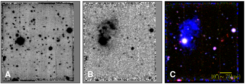
Figure 1: Discovery images of the ELAN around the quasar SDSS J1020$+$1040. (A) white-light image of the combined exposures showing the whole FOV of our observations. Vertical stripes with slightly lower signal-to-noise are visible in this image due to our observing strategy (see section 2 for details). (B) NB image of 40 Å centred at the redshift $z=3.167$ of the extended Ly$\alpha$ emission. The image has been smoothed with a gaussian kernel of $0.6\arcsec$ (or 3 pixels). (C) RGB image composed of the NB image, and two intermediate continuum bands free of line emissions at the redshift of SDSS J1020$+$1040 of about $200$ Å centred at $5400$ Å and $8237$ Å, respectively. North is up, East is to the left.

3.1 Search for Companion Sources: Hints of an Overdensity

To identify galaxies at the same redshift of the quasar, we use two complementary approaches. We search for i) compact continuum sources and ii) compact Ly$\alpha$ emitters whose continuum might have been too faint to be detected in the former case. We then determine the redshifts by looking for lines or continuum breaks (if any). This analysis led to the discovery of four companions of which we show the positions in both the white-light image and in the NB image in Fig. 2, and list them in Table LABEL:tabPos. Further, we show their spectra in Fig. 3.

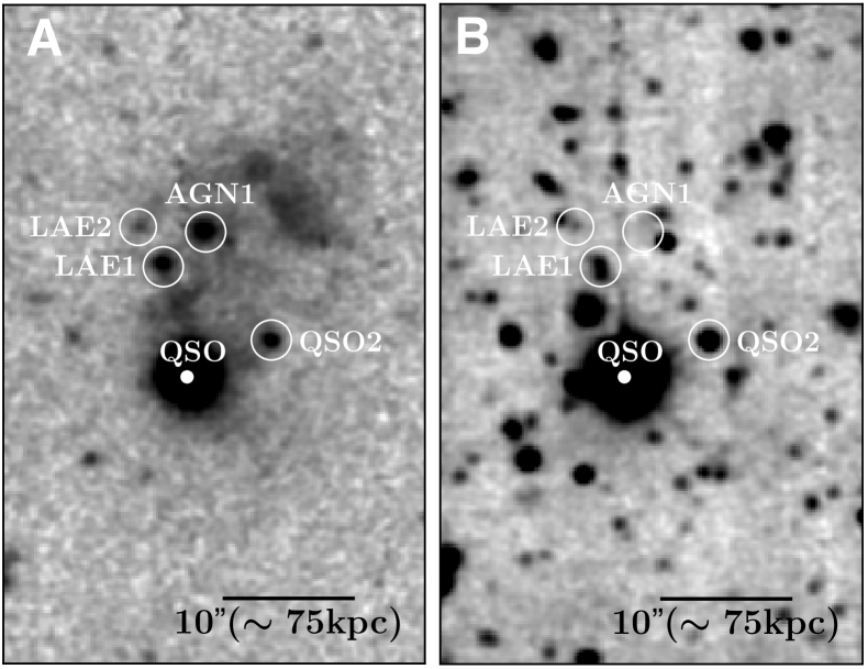
Figure 2: Position of the compact sources associated with the ELAN. (A) Portion of the $40$ Å NB image matching the Ly$\alpha$  line of the quasar SDSS J1020$+$1040 extracted from the MUSE datacube. (B) Portion of the white-light image obtained by collapsing the MUSE datacube. In both panels, the positions of the objects associated with the ELAN are indicated. North is up, East is to the left.

Table 1: Positions and $i$-mag for the associated sources QSO2, AGN1, LAE1, and LAE2.

Source	RA	Dec	Separation	$i$-mag
	(J2000)	(J2000)	(arcsec)	(AB)
QSO2	10:20:09.58	+10:40:02.30	6.8	$24.30\pm 0.02$
AGN1	10:20:09.92	+10:40:13.93	11.3	$>28.6$
LAE1	10:20:10.15	+10:40:11.53	9.1	$25.45\pm 0.05$
LAE2	10:20:10.24	+10:40:14.13	11.9	$>27.0$

More specifically, the companions have been found as follows. First, we use the white-light image shown in Fig. 1 as a deep continuum detection image and construct a catalogue of source candidates. Specifically, we run SExtractor (Bertin & Arnouts 1996) with a detection area of 5 pixels and a threshold of 2$\sigma$ above the background root-mean-square. We then use the segmentation map generated by SExtractor as a mask to extract 1D spectra for each identified source from the final MUSE datacube. Next, we inspected the 1D spectra to identify emission or absorption lines at the redshift of SDSS J1020$+$1040. Of all the 177 continuum detected sources in the deep white-light image, only two are clearly at redshifts similar to SDSS J1020$+$1040. These are a quasar, referred to as QSO2, and a strong Ly$\alpha$ emitter (EW${}_{\rm rest}=105$ Å), referred to as LAE1, at projected distances of $51.7$ kpc ($6.8\arcsec$) and $69.2$ kpc ($9.1\arcsec$) from SDSS J1020$+$1040, respectively (Fig. 2). We evaluate the redshift of QSO2 with the same approach as for SDSS J1020$+$1040  (see appendix A), i.e. following Shen et al. (2016). Specifically, we estimate the peak of the C iv line, as specified in Shen et al. (2016), and obtained $z=3.158$. With a measured $\lambda L_{1700\textup{\AA}}=(5.0\pm 0.9)\times 10^{43}$ erg s^-1 for QSO2, we estimate an expected shift of +173 km s^-1 for C iv with respect to systemic. We thus obtain a redshift of $z=3.156\pm 0.006$ for QSO2, where we took into account the systematic uncertainty of $415$ km s^-1 in the error estimate (Shen et al. 2016). Bearing in mind the uncertainties on the redshift determination for both quasars, QSO2 seems to have a blueshift of 576 km s^-1 with respect to SDSS J1020$+$1040.

For LAE1, we have obtained a redshift of $z=3.168\pm 0.001$ by fitting its Ly$\alpha$ emission line with a gaussian (despite the presence of a red tail in its shape). For both QSO2 and LAE1, we have extracted an equivalent $i$-band SDSS magnitude from the MUSE datacube, obtaining $24.30\pm 0.02$ and $25.45\pm 0.05$, respectively. These sources are therefore much fainter than SDSS J1020$+$1040 ($i$=17.98, fiber magnitude).

Secure redshifts could not be obtained for any of the other continuum-detected sources, e.g. no presence of emission lines, no continuum breaks. In particular, note that continuum sources that happen to be at the same location of the ELAN, show faint line emission at the wavelength of the Ly$\alpha$ emission of the ELAN itself. Given that these faint continuum sources are not visible as compact Ly$\alpha$ emitters in the NB image (see Fig. 2), and that they do not show other emission lines, we ascribe the emission to the nebula.

As stated earlier, we also search for associated compact line emitters whose faint continua were not detected in the deep white-light image. Specifically, we use the 40 Å NB image presented in Fig. 1 as a detection image to construct a catalogue of source candidates. We run SExtractor with a detection area of 5 pixels and a threshold of 2$\sigma$ above the background root-mean-square. Next we matched this line-emitter catalog to our catalog of continuum sources from the foregoing discussion, and removed all those with continuum detections. The segmentation map of the remaining sources was used as a mask to extract 1D spectra from the final MUSE datacube. This approach led to the identification of two Ly$\alpha$ emitters at a redshift similar to SDSS J1020$+$1040, AGN1 at $z=3.179\pm 0.001$ (EW${}_{\rm rest}>168$ Å) at $11.3\arcsec$ ($\sim 85.9$ kpc), and LAE2 at $z=3.167\pm 0.001$ (EW${}_{\rm rest}>29$ Å) at $11.9\arcsec$ ($\sim 90.4$ kpc) (Fig. 2). AGN1 also exhibits a C iv  emission line, and tentative evidence for He ii and N v  emission lines, all indicative of a hard-ionizing source, making this source most likely a type-2 AGN. Indeed, its line ratios are in good agreement with type-2 AGN reported in the literature as shown in Fig. 4 (Nagao et al. 2006; McCarthy 1993; Humphrey et al. 2008). Given its redshift, AGN1 has a velocity shift of 864 km s^-1 with respect to SDSS J1020$+$1040. Note that AGN1 does not have a fully gaussian Ly$\alpha$ line, although redshifts determined from both Ly$\alpha$ and C iv agree within their uncertainties. On the other hand, LAE2 shows strong Si iv emission, also requiring a hard-ionizing source (ionization energy of I${}_{\rm SiIV}=33.49$ eV; Draine 2011). However, we don’t detect other high ionization lines (He ii, C iv, N v, C iii]) which typically accompany Si iv in AGN spectra (e.g., McCarthy 1993; Humphrey et al. 2008; Hainline et al. 2011; Lacy et al. 2013). To our knowledge, there are no sources reported in the literature with only Ly$\alpha$ and Si iv detected. In the population of Lyman break galaxies (LBGs; e.g., Shapley et al. 2003) or LAEs characterized by similar strong Ly$\alpha$ emission as LAE2, Si iv is usually observed in absorption (e.g., 4th quartile in Shapley et al. 2003). We show the discrepancy between the line ratios for LAE2 and the population of type-2 AGN and LBGs in Fig. 5. LAE2 thus seems a clear outlier for both type-2 AGN and LBGs. However, we argue that the strong Si iv emission should be a signature of powering mechanisms more similar to an AGN. The nature of LAE2 remains unclear, and follow up studies are needed. Intriguingly, Dey et al. (2005), while studying a LAB at $z=2.656$, reported the detection of an emission line at $\lambda=5081.6$ Å, which could have been an improbable blueshifted Si iv line, or an interloper as the author suggested. The information for the three sources with narrow emission lines are summarized in Table LABEL:tabCompactSources.

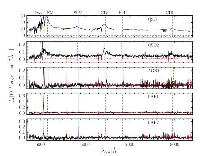
Figure 3: One-dimensional spectra of the strong Ly$\alpha$ emitters associated with the ELAN. The 1D spectrum of SDSS J1020$+$1040 has been extracted in a $1.5\arcsec$ radius circular aperture, while the other four spectra have been extracted within the 2$\sigma$ isophote of each source (see section 3.1). For each object, the red dashed line shows the noise spectra extracted within the same aperture. At long wavelengths the MUSE spectra become noisier due to the presence of residuals of stronger and numerous sky-lines (more evident for the fainter sources). The blue dashed lines indicate the location of the typical strong ultra-violet emission lines encountered in quasar’s spectra. The individual y-axes have been scaled for presentation. QSO2 and AGN1 have been classified as AGN. Having a strong Si iv line in emission, LAE2 is a clear outlier in comparison to typical Ly$\alpha$ emitters at this redshift (see section 3.1 and Fig. 5).

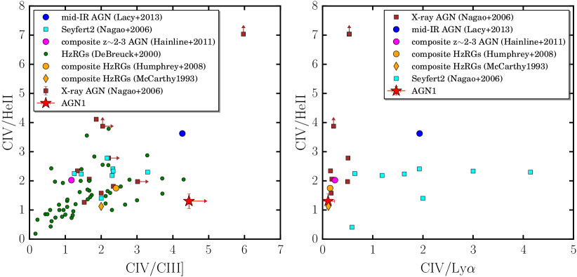
Figure 4: Comparison between AGN1 and the Type-2 AGN in the literature. The line-ratios of AGN1 (red star) are compared to other Type-2 AGN from the literature in the C iv/He ii vs. C iv/C iii] diagram (left), and in the C iv/He ii vs. C iv/Ly$\alpha$ diagram (right). We show the values for (i) individual HzRGs (green circles; De Breuck et al. 2000), (ii) individual narrow-line X-ray sources (brown squares; Nagao et al. 2006), (iii) individual Seyfert-2s (cyan squares; Nagao et al. 2006), (iv) two composites for HzRGs (orange diamond; McCarthy 1993; and orange circle, Humphrey et al. 2008), (v) a composite of narrow-lined AGN at $z\sim 2-3$ (magenta; Hainline et al. 2011), and (vi) a composite for mid-IR selected Type-2 AGN (blue circle; Lacy et al. 2013). To avoid confusion, we only show the errorbars for our data point. The typical uncertainties on the line ratios from the literature are of the order of 0.5-1. Overall, AGN1 seems to agree with the type-2 AGN reported in the literature.

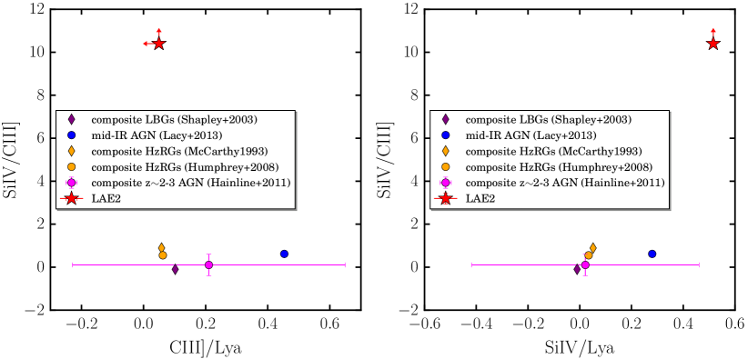
Figure 5: Comparison between LAE2 and the Type-2 AGN and LBGs in the literature. The line-ratios of LAE2 (red star) are compared to Type-2 AGN and LBGs from the literature in the Si iv/C iii] vs. C iii]/Ly$\alpha$ diagram (left), and in the Si iv /C iii] vs. Si iv/Ly$\alpha$ diagram (right). We show the values for (i) two composites for HzRGs (orange diamond, McCarthy 1993; and orange circle, Humphrey et al. 2008), (ii) a composite of narrow-lined AGN at $z\sim 2-3$ (magenta; Hainline et al. 2011), (iii) a composite for mid-IR selected Type-2 AGN (blue circle; Lacy et al. 2013), and (iv) a composite for bright Ly$\alpha$ emitting LBGs (EW${}_{\rm Ly\alpha}^{\rm rest}=52.63\pm 2.74$, 4th quartile in Shapley et al. 2003). Note that LBGs have Si iv in absorption and thus their ratio on this plot is negative. LAE2 is a clear outlier.

Table 2: Information on the emission lines detected in the spectrum of AGN1, LAE1, and LAE2.

Line	Line Center	Redshift	Line Flux	Continuum Flux	EWrest	Line Width
	(Å)		(10-17 erg s-1 cm-2)	(10-20 erg s-1 cm-2 Hz-1)	(Å)	(km s-1)
AGN1 ($\langle z\rangle=3.179\pm 0.001$, d$=85.9$ kpc)
Ly$\alpha$	5080.51$\pm$0.03	3.179$\pm$0.001	9.90$\pm$0.08	-4.4$\pm$7.0	$>$168	232.4$\pm$1.9
C iv	6474.6$\pm$0.6	3.180$\pm$0.001	1.09$\pm$0.08	-3.2$\pm$3.0	$>$42	213$\pm$26
He ii	6854.2$\pm$0.2	3.179$\pm$0.001	0.83$\pm$0.04	-2.9$\pm$4.0	$>$25	156$\pm$10
LAE1 (d$=69.2$ kpc)
Ly$\alpha$	5067.68$\pm$0.05	3.168$\pm$0.001	5.49$\pm$0.06	12.6$\pm$9.8	104.96$\pm$0.78	239.6$\pm$2.8
LAE2 ($\langle z\rangle=3.167\pm 0.001$, d$=90.4$ kpc)
Ly$\alpha$	5064.9$\pm$0.1	3.166$\pm$0.001	2.41$\pm$0.07	-1.4$\pm$9.8	$>$29	186.9$\pm$6.0
Si iv	5846.42$\pm$0.07	3.167$\pm$0.001	1.24$\pm$0.04	-3.7$\pm$3.6	$>$41	90.6$\pm$3.9

The presence of three confirmed AGN within 90 projected kpc makes this system similar to the other two known physical quasar triplets discovered at lower redshifts (Djorgovski et al. 2007; Farina et al. 2013). In addition, given the presence of unusual compact emitters embedded in the ELAN, it might resemble the properties of the so far only known quadruple quasar (Hennawi et al. 2015), known to be embedded in a bright ELAN as well. It is thus interesting to compare the environment of that system with SDSS J1020$+$1040. Hennawi et al. (2015) show that the bright quasar SDSS J084158.47+392121.0 (henceforth SDSS J0841) in their system inhabits a clear overdensity of LAEs, exceeding the average protoclusters, i.e. high-redshift radio galaxies (HzRGs) and Lyman-Alpha Blobs (LABs; e.g., Yang et al. 2009), by a factor of $\gtrsim 20$ for $R<200$ kpc and by $\sim 3$ on scales of $R\simeq 1$ Mpc. To allow a comparison with studies of HzRGs and LABs, the analysis of Hennawi et al. (2015) relies on the LAEs selected to have $EW_{\rm rest}>20$Å  and with $f_{\rm Ly\alpha}>4.0\times 10^{-17}$ erg s^-1 cm^-2. Given our pointing strategy and the MUSE FOV, we are able to fully probe the environment only within $R\lesssim 122$ kpc (or $\lesssim 16\arcsec$) from SDSS J1020$+$1040. Within this region, following the same selection criteria of Hennawi et al. (2015), we find 3 objects (2 of which are AGN), while SDSS J0841 has 4 objects (2 of which are AGN), suggesting that the system studied here inhabits a similar overdensity on small $\lesssim 100$ kpc scales as SDSS J0841, and making it a rare overdense system as well. A follow-up narrow-band study of a wider field around SDSS J1020$+$1040 is needed for a full comparison. However, the similarity on small scales with SDSS J0841, together with the presence of multiple AGN, make SDSS J1020$+$1040 likely to be the progenitor of a very massive object.

Finally, we note that the other two ELANe so far discovered are also associated to multiple AGN and overdensities of galaxies (Cantalupo et al. 2014; Cai et al. 2017). Cantalupo et al. (2014) report the discovery of an ELAN associated to the quasar UM 287 ($z=2.279$) and a fainter companion quasar. Further, Cai et al. (2017) unveil a bright ELAN at $z=2.319\pm 0.004$ displaced by $33.1\arcsec$ from the quasar SDSS J144121.66+400258.8 ($z=2.311\pm 0.006$) by targeting the density peak of the large-scale structure BOSS1441 (Cai et al. 2016). Showing extended C iv and He ii in emission, this ELAN probably hosts an additional obscured AGN which is powering the nebula through an outflow and/or photionization (Cai et al. 2017). More generally, it has been argued that the presence of a giant Ly$\alpha$ nebula (wether is an ELAN, a LAB or associated to an HzRG) is physically connected to the location of overdensities of galaxies and AGN (Matsuda et al. 2005, 2009; Saito et al. 2006; Venemans et al. 2007; Prescott et al. 2008; Yang et al. 2009; Hennawi et al. 2015).

3.2 The Enormous Lyman-Alpha Nebula

In Fig. 1 we have shown an NB image of the ELAN around the quasar SDSS J1020$+$1040. In this section we report how we analysed the final MUSE datacube to constrain this extended Ly$\alpha$ emission, while in appendix C we explain how we tested the reliability of our approach.

3.2.1 Empirical PSF subtraction and Moments of the Flux Distribution

We extracted the properties of the Ly$\alpha$ emission using the CubExtractor package, as explained in Borisova et al. (2016). Briefly, we have first subtracted the quasar PSF to remove any contamination from the unresolved QSO on large scales, and then we have characterised the properties of the ELAN by calculating the moments of the flux distribution.

More specifically, the subtraction of the PSF has been performed using the CubePSFSub algorithm within CubExtractor, which empirically reconstructs the PSF of the quasar in user-defined wavelength layers within the MUSE datacube. For each wavelength layer, the empirical PSF image is obtained as a pseudo-NB image, it is rescaled to the flux within $5\times 5$ pixels (or $1\arcsec\times 1\arcsec$) around the quasar position, and then subtracted (see Borisova et al. 2016 for more details). In our case, we have used a wavelength layer of 150 spectral pixels ($187.5$Å), shown to be optimal for the case of extended emission around quasars (Borisova et al. 2016). Note that this method is not reliable in the central $1\arcsec\times 1\arcsec$ region used for the PSF rescaling, leading to residuals on these scales (Borisova et al. 2016). However, in appendix C we show that the PSF subtraction following a different algorithm does not change our results (Husemann et al. 2013). In addition to the PSF subtraction, we have removed all the continuum-detected sources from the datacube using the CubeBKGSub algorithm, which uses a fast median-filtering approach (see Borisova et al. 2016 for more details).

We then use CubExtractor to identify the diffuse Ly$\alpha$ emission by searching for regions with a minimum “volume” of 10,000 voxels (volume pixels) above a signal-to-noise ${\rm S/N}>2$ within the MUSE datacube. In this way, we are left with a three-dimensional mask which indicates the voxels associated with the extended Ly$\alpha$ emission around the quasar SDSS J1020$+$1040. We used this mask to obtain an “optimally extracted” NB image by integrating the flux along the wavelength direction for only the voxels belonging to the nebulosity. Each pixel itself in the obtained 2D-image thus represents a narrow-band filter, whose width is set by the ${\rm S/N}=2$ threshold. We have then added to the “optimally extracted” NB image a ’background’ layer of 40 Å around $z=3.167$ (central wavelength of the nebula for region closer to QSO position) to recreate the noise for a NB image with the wavelength range equal to the maximum width of the nebulosity, i.e the maximum width of the 3-D mask previously obtained. In panel A of Fig. 6 we show this optimally extracted NB image, which clearly reveals that this Ly$\alpha$ nebula is one of the so far brightest and largest known around radio-quiet quasars. The nebula has an average SB${}_{\rm Ly\alpha}=6.04\times 10^{-18}\,{\rm\,erg\,s^{-1}\,cm^{-2}\,arcsec^{-2}}$ (within the $2\sigma$ isophote). Note that an “optimally extracted” image does not allow a visual estimate of the noise as it depends on the number of layers at each spatial position. Hence, to enable a better interpretation we show in Fig. 6 the signal-to-noise contours for $S/N=2,4,10,20,30,50$, and $100$, estimated through variance propagation accounting for the number of layers along each pixel position (see Borisova et al. 2016).

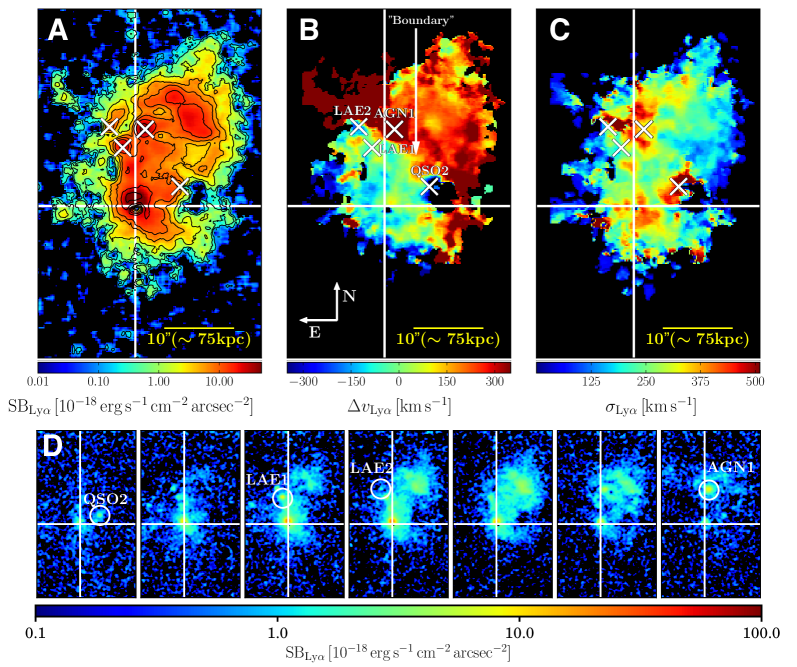
Figure 6: The enormous Ly$\alpha$ nebula (ELAN) surrounding the quasar SDSS J1020$+$1040. (A) “optimally-extracted” Ly$\alpha$ surface brightness map obtained after subtraction of the quasar point-spread-function (PSF) and continuum in the final MUSE datacube (see section 3.2.1). The black contours indicate the isophotes corresponding to a signal-to-noise ratio of ${\rm S/N}=2,\,4,\,10,\,20,\,30,\,50$, and $100$. This image reveals an extremely bright nebula (SB${}_{\rm Ly\alpha}\sim 10^{-17}{\rm\,erg\,s^{-1}\,cm^{-2}\,arcsec^{-2}}$) extending on 100 kpc scales on the NW side of the quasar. Additional four strong Ly$\alpha$ emitters (diagonal crosses) are associated with SDSS J1020$+$1040, and the ELAN. Two of these sources have been spectroscopically confirmed as AGN (Fig. 3), making this system the third known quasar triplet. (B) flux-weighted velocity-shift map with respect to the systemic redshift of the quasar SDSS J1020$+$1040  obtained from the first-moment of the flux distribution. A velocity shear between the SE and NW portion of the nebula is evident. The transition region is referred to as the “Boundary”. (C) velocity dispersion map obtained from the second-moment of the flux distribution. Regions of higher dispersion ($\sigma_{\rm Ly\alpha}\approx 430$ km s^-1) are visible in proximity of the three AGN, but overall the Ly$\alpha$ nebula shows quiescent kinematics ($\sigma_{v}<270$ km s^-1). (D) Each cut-out image (same size as A, B, and C) shows the surface brightness map of the ELAN within a 3.75 Å layer ($3\times$ MUSE sampling) in the wavelength range 5058 Å $\lesssim\lambda\lesssim$ 5084 Å (from left to right). In all of the panels (A, B, C, D) the large white cross indicates the position of the quasar SDSS J1020$+$1040  prior to PSF subtraction.

Further, the PSF subtracted image reveals a bright peak for the Ly$\alpha$ emission $\simeq 1\arcsec$ to the North of the quasar SDSS J1020$+$1040  (Fig. 6). The Ly$\alpha$ emission at this location show a much narrower profile ($\sigma_{\rm Ly\alpha}=316.4\pm 7.9$ km $s^{-1}$) than the more complex quasar’s broad Ly$\alpha$ line blended together with the N v emission. This comparison is shown in Fig. 7. Given the great differences in the line shapes, we are therefore confident that the bright emission in close proximity to the quasar SDSS J1020$+$1040 cannot constitute a PSF subtraction residual. This bright knot may represent the extended emission line regions (EELR; Stockton et al. 2006) associated with quasars, i.e. narrow emission-line regions extending for tens of kpc around AGN, and thought to be mainly powered by the central bright source or star-formation from the host-galaxy (e.g., Husemann et al. 2014). Interestingly, this emission is at the redshift of $z=3.167\pm 0.001$, and is connected to the emission on larger scales. This occurrence thus confirm that the Ly$\alpha$ nebula and the quasar SDSS J1020$+$1040 are at the same redshift, once the known uncertainties are taken into account (see appendix A).

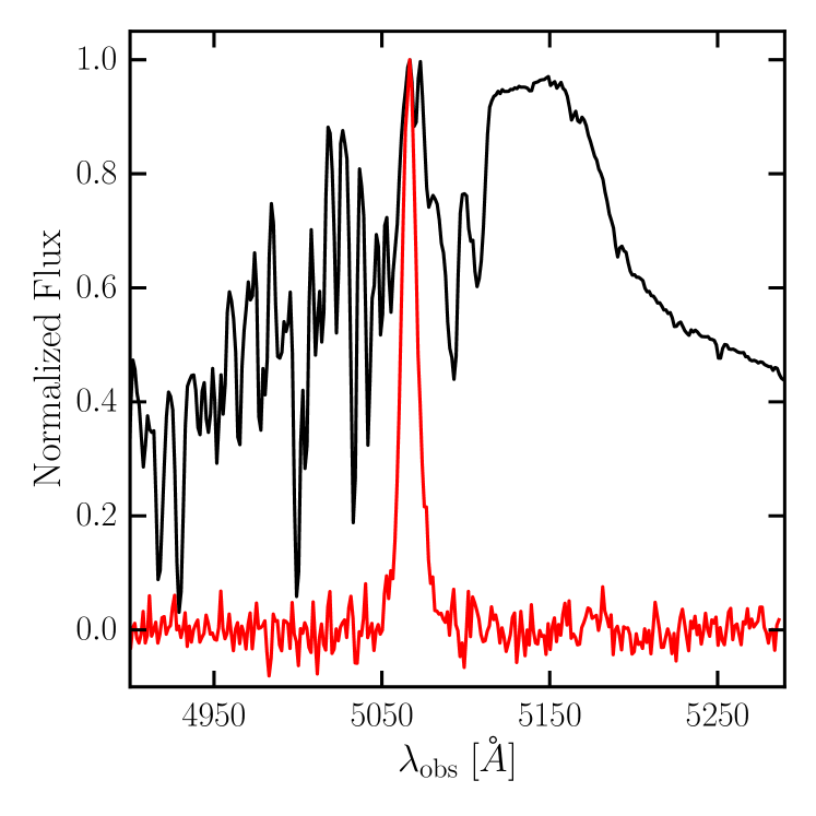
Figure 7: Ly$\alpha$ line shape for the quasar SDSS J1020$+$1040 and the peak of the ELAN. We compare the Ly$\alpha$ line emission of the quasar (black) and of the peak of the ELAN (red), i.e. at $\approx 1\arcsec$ from the quasar. The spectrum of the peak of the ELAN has been extracted within a circular aperture of $2\arcsec$ radius centred at $\alpha=155.0428$ deg and $\delta=10.6679$ deg (Region 3 in Fig. 14). Both spectra have been normalized to their maximum. The ELAN emission is much narrower than the complex Ly$\alpha$ emission of the quasar SDSS J1020$+$1040. We are thus confident that the peak of the ELAN close to the quasar position is not due to PSF residuals.

We then use the aforementioned three-dimensional mask to analyse the kinematics of the Ly$\alpha$ emitting gas. Specifically, to derive the centroid velocity and the width of the emission line, we have computed at each spatial location the first and second moment of the flux distribution only for the voxels selected by the mask. The use of only the selected “volume” should minimise the effect of the noise for this approach.

Panel B in Fig. 6 shows the flux-weighted centroid of the Ly$\alpha$ emission throughout the ELAN with respect to the systemic redshift of SDSS J1020$+$1040. The ELAN clearly exhibits a significant velocity shear as one progresses from its SE edge to the NW. The southern half of the ELAN shows systematically blueshifted velocities (by $\approx 300$ km s^-1) compared to its northern half, and there is a relatively sharp discontinuity across the “boundary”. Panel C in Fig. 6 shows the flux-weighted standard deviation of the emission. The values are relatively small, $\sigma_{v}<270$ km s^-1 and are nearly consistent with the spectral resolution of MUSE. One concludes that the motions within this ELAN are highly coherent, and have amplitudes consistent with being gravitational motions within a dark matter halo hosting a quasar. This high coherence of the velocity field can be greatly appreciated by looking at panel D in Fig. 6. This panel dissects the ELAN presented in panel A, B, and C in a sequence of narrow-band images of $3.75$ Å ($3\times$ MUSE sampling) in the wavelength range $5058$ Å $\lesssim\lambda\lesssim$ $5084$ Å. We will further discuss this observed velocity shear in section 4.1.

3.2.2 The Enormous Lyman-Alpha Nebula in He ii and C iv 

To try to mitigate the possible uncertainties that arise from the use of the Ly$\alpha$ emission as a unique diagnostic (section 4.2.1), our QSO MUSEUM survey (Arrigoni Battaia et al., in prep.) specifically targets $z\sim 3$ quasars to be able to cover other strong rest-frame ultraviolet lines beside Ly$\alpha$. In particular, it has been shown that the C iv $\lambda 1549$ and He ii $\lambda 1640$ lines are important indicators that may constrain the density, ionization state, metallicity, and the importance of scattering within the emitting gas (Nagao et al. 2006; Prescott et al. 2009; Humphrey et al. 2008; Prescott et al. 2015a; Arrigoni Battaia et al. 2015a; Arrigoni Battaia et al. 2015b). Further, as described in detail in Arrigoni Battaia et al. (2015a); Arrigoni Battaia et al. (2015b), these emission lines can disentangle the powering mechanisms for the Ly$\alpha$ emission, such as photoionization from AGN or star-formation (Arrigoni Battaia et al. 2015a and references therein), scattering of Ly$\alpha$ photons (e.g., Dijkstra & Loeb 2008; Cen & Zheng 2013), shock-heated gas in superwinds (e.g., Taniguchi & Shioya 2000; Mori et al. 2004; Cabot et al. 2016), or cooling radiation (e.g., Yang et al. 2006; Rosdahl & Blaizot 2012). Such mechanisms can also act together, and additional diagnostics might be needed to characterise the different contributions (e.g. polarization of the Ly$\alpha$ line Prescott et al. 2011). Here we report our observations at the C iv and He ii expected wavelengths, while we discuss the powering mechanisms for the ELAN around SDSS J1020$+$1040 in section 4.3.

To assess the presence of extended C iv and He ii in our data, we proceed in two ways. First, using CubExtractor, we have searched for connected voxels above a signal-to-noise ${\rm S/N}>2$ at the wavelength of the two emission lines, on unsmoothed data, and leaving the minimum “volume” unconstrained, so that less extended emission than the enormous Ly$\alpha$ emission would have also been detected. This approach led to the detection of compact unresolved emission close to the quasar PSF residuals, but no extended emission has been detected at the expected redshift, with only a hint for extended emission in the C iv line if the ${\rm S/N}>2$ constrain is relaxed. Secondly, given the possibility of a velocity shift between the Ly$\alpha$ line emission and the C iv and He ii emission, we have searched the datacube with the same approach within a window of 2000 km s^-1 on both side of the expected location. This approach has also not resulted in the detection of the two lines on large scales. Here, we have thus decided to present our data by simply constructing two narrow-band images of 30 Å centred at the expected wavelength of the two emission lines at $z=3.167$ (redshift of the peak of the Ly$\alpha$ nebula; section 3.2.1), i.e. $\lambda=6454.7$ Å  and $\lambda=6833.9$ Å, respectively for C iv and He ii . The NB images are obtained by collapsing the final datacube, after the quasar PSF and the continuum sources have been removed (as explained in section 3.2.1).

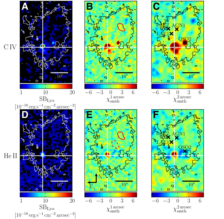
Figure 8: Narrow-band images extracted at the expected wavelengths for C iv and He ii. (A) C iv surface brightness map for a $30$ Å NB image obtained by collapsing the final MUSE datacube around $z=3.167$ (redshift of the ELAN), after quasar PSF and continuum subtraction. (B) $\chi_{\rm smth}$ image for the same wavelength range (expected C iv location) obtained using a Gaussian kernel with FWHM$=1\arcsec$ as explained in section 3.2.2. The red contour highlights the ${\rm S/N}=50$ isophote for the Ly$\alpha$ emission used to extract the line ratios for the clump at $\approx 120$ kpc from SDSS J1020$+$1040. (C) $\chi_{\rm smth}$ image for the same wavelength range (expected C iv location) obtained using a Gaussian kernel with FWHM$=2\arcsec$ as explained in section 3.2.2. (D), (E), (F) Same as for (A), (B), and (C), respectively, but for the He ii line. In (E), the dashed red contour indicates the portion of the ELAN used in the analysis that resulted in Fig. 27. No clear extended emission in C iv and He ii is associated to the ELAN down to our sensitivity limits. However the aggressive smoothing seems to suggest very faint extended C iv emission in the South-West direction from SDSS J1020$+$1040.

Panels A and D of Fig. 8 show the surface brightness maps for the NB images of the giant Ly$\alpha$ nebula in the C iv and He ii lines after smoothing the data with a Gaussian kernel of 1 arcsec. These images have a 2$\sigma$ SB limit within a square arcsecond of SB${}_{\rm lim}^{\rm CIV}=1.05\times 10^{-18}{\rm\,erg\,s^{-1}\,cm^{-2}\,arcsec^{-2}}$, and SB${}_{\rm lim}^{\rm HeII}=1.18\times 10^{-18}{\rm\,erg\,s^{-1}\,cm^{-2}\,arcsec^{-2}}$, while the depth achieved for individual channels at these wavelength is SB${}_{\rm lim}=2.25\times 10^{-19}{\rm\,erg\,s^{-1}\,cm^{-2}\,arcsec^{-2}}$, and SB${}_{\rm lim}=2.69\times 10^{-19}{\rm\,erg\,s^{-1}\,cm^{-2}\,arcsec^{-2}}$, respectively for C iv and He ii . To indicate the significance of the mild detection of the compact emission and to search for evidence of faint emission on large scales, we have computed a smoothed $\chi$ image following the technique in Hennawi & Prochaska (2013) and Arrigoni Battaia et al. (2015a), for two Gaussian kernels with FWHM$=1\arcsec$ and FWHM$=2\arcsec$, respectively. To obtain these images, we proceed as follows. First, we obtain an unsmoothed NB image $I$ of 30 Å by collapsing the final MUSE datacube at the wavelength of interest. Then, we smooth this image using the Gaussian kernel, obtaining $I_{\rm smth}$. Next, from the variance cube we have computed the unsmoothed variance image $\sigma^{2}_{\rm unsmooth}$ for each NB image, and obtained the smoothed sigma image $\sigma_{\rm smth}$ by propagating the variance image of the unsmoothed data:

$$\sigma_{\rm smth}=\sqrt{{\rm CONVOL}^{2}[\sigma_{\rm unsmooth}^{2}]},$$ (1)

where the CONVOL² operation denotes the convolution of the variance image with the square of the Gaussian kernel. Thus, the smoothed $\chi$ image is defined by

$$\chi_{\rm smth}=\frac{I_{\rm smth}}{\sigma_{\rm smth}}.$$ (2)

These $\chi_{\rm smth}$ maps are more effective in visualising the presence of extended emission.

From Fig. 8 it is clear that C iv emission is only definitively detected in close proximity of the two quasars, SDSS J1020$+$1040 and its companion, while the He ii emission is seen clearly only close to SDSS J1020$+$1040 (North direction). In the case of SDSS J1020$+$1040, the additional emission lines have their maxima at the same position of the peak of the Ly$\alpha$ emission at $\approx 1\arcsec$ from SDSS J1020$+$1040. Being narrow and at the same redshift of the quasar, this small-scale emission is thus probably due to the so-called EELR around the bright quasar (see section 3.2). Deeper data at higher spatial resolution are needed to explore in further detail the presence, kinematics, and geometry of the C iv and He ii line-emissions on these small scales. Such observations will be feasible once the adaptive-optic system for MUSE becomes available (GALACSI; Stuik et al. 2006).

In addition, there is the hint (very low significance in the unsmoothed data) in the C iv map for extended emission in the South-West direction of SDSS J1020$+$1040. Given the faint levels for this emission, we are not able to investigate if it traces the same kinematics as the Ly$\alpha$ emission in this region. Deeper observations are needed to confirm this emission and eventually compare it with the Ly$\alpha$ emission.

Finally, as they can be used to infer the physical properties of the gas in emission, we report here the line ratios between C iv, He ii, and Ly$\alpha$, and discuss in section 4.3 their implications. Specifically, given that we do not have a detection in C iv and He ii on large scales, we compute the 5$\sigma$ SB limits within the ${\rm S/N}=2$ isophote defined by the Ly$\alpha$ emission (see black contour in Fig. 8), which corresponds to an area on the sky of 609.36 arcsec². We obtain SB${}_{\rm HeII}<1.2\times 10^{-19}{\rm\,erg\,s^{-1}\,cm^{-2}\,arcsec^{-2}}$, and SB${}_{\rm CIV}<1.1\times 10^{-20}{\rm\,erg\,s^{-1}\,cm^{-2}\,arcsec^{-2}}$, resulting in He ii/Ly$\alpha$$<0.020$, and C iv/Ly$\alpha$$<0.018$ when using the average SB${}_{\rm Ly\alpha}=(6.04\pm 0.26)\times 10^{-18}{\rm\,erg\,s^{-1}\,cm^{-2}\,arcsec^{-2}}$ for the whole nebula. We compute the $5\sigma$ limits also for the bright clump at a projected distance of $\approx 120$ kpc from SDSS J1020$+$1040. In particular, we use the isophote within which the Ly$\alpha$ emission has ${\rm S/N}>50$ (region indicated with a red contour in Fig. 8, area of 13.4 arcsec²) finding SB${}_{\rm HeII}<8.1\times 10^{-19}{\rm\,erg\,s^{-1}\,cm^{-2}\,arcsec^{-2}}$, and SB${}_{\rm CIV}<7.2\times 10^{-19}{\rm\,erg\,s^{-1}\,cm^{-2}\,arcsec^{-2}}$, resulting in He ii/Ly$\alpha$$<0.045$, and C iv/Ly$\alpha$$<0.039$ when using the average SB${}_{\rm Ly\alpha}=(1.81\pm 0.08)\times 10^{-17}{\rm\,erg\,s^{-1}\,cm^{-2}\,arcsec^{-2}}$ within the same region. Further, we also compute the line ratios for the detected EELR close to SDSS J1020$+$1040 and obtained SB${}_{\rm HeII}=(7.24\pm 0.35)\times 10^{-18}{\rm\,erg\,s^{-1}\,cm^{-2}\,arcsec^{-2}}$, and SB${}_{\rm CIV}=(1.11\pm 0.05)\times 10^{-17}{\rm\,erg\,s^{-1}\,cm^{-2}\,arcsec^{-2}}$, resulting in He ii/Ly$\alpha$$=0.12\pm 0.01$, and C iv/Ly$\alpha$$=0.18\pm 0.01$ when using the average SB${}_{\rm Ly\alpha}=(6.08\pm 0.27)\times 10^{-17}{\rm\,erg\,s^{-1}\,cm^{-2}\,arcsec^{-2}}$ at this location. Fig. 9 summarizes our datapoints and compares them to data in the literature for radio-quiet extended Ly$\alpha$ nebulosities at high redshift. Our data for the whole ELAN are consistent with the non-detections usually reported in the literature for radio-quiet Ly$\alpha$ nebulae (e.g., Arrigoni Battaia et al. 2015a). While the values of the EELR are in agreement with the detections in the literature for nebulae currently explained as powered by an enshrouded AGN (i.e. Dey et al. 2005; Cai et al. 2017).

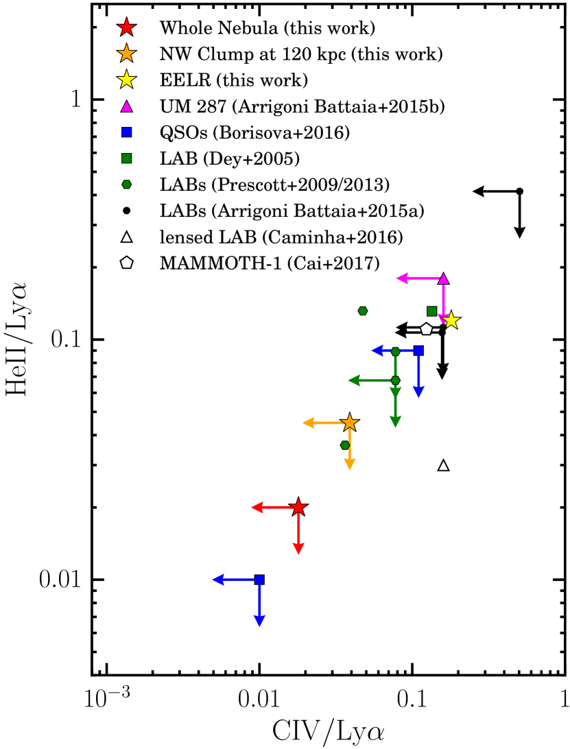
Figure 9: He ii/Ly$\alpha$ vs. C iv/Ly$\alpha$ log-log plot for radio-quiet Ly$\alpha$ nebulae. Our upper limits of the He ii/Ly$\alpha$ and C iv/Ly$\alpha$ ratios for the whole Ly$\alpha$ nebula (red), the NW clump at ${\approx 120}$ kpc (orange) and the datapoint for the EELR (yellow) here studied are compared with data available in the literature for other radio-quiet Ly$\alpha$ nebulae. Specifically, we show data for (i) LABs from Prescott et al. (2009, 2013); Dey et al. (2005), Caminha et al. (2016), and Arrigoni Battaia et al. (2015a) (only the most and less stringent data-points); (ii) Ly$\alpha$ nebulae around radio-quiet QSOs from Arrigoni Battaia et al. (2015b) and from Borisova et al. (2016) (only the most and less stringent data-points); (iii) the MAMMOTH-1 ELAN (Cai et al. 2017). The errorbars for both ratios ($\sigma=0.01$) for our EELR datapoint are smaller than the size of the symbol used.

4 Discussion

In this section we first show how the velocity shear observed within the ELAN around SDSS J1020$+$1040 is remarkably similar to a rotation-like pattern and discuss the favoured interpretation in light of the current data. Secondly, we consider in turn alternative scenarios for the presence of such a velocity shear. Finally, we discuss the possible powering mechanisms that could give rise to such bright Ly$\alpha$ emission on 100 kpc scales, with no extended He ii and C iv emission down to our current SB limits.

4.1 The favoured interpretation: witnessing mass assembly around a $z\sim 3$ quasar

We better highlight the velocity shear presented in Fig. 6 and section 3.2 with two complementary views. First, we present the velocities with respect to the quasar systemic redshift along three parallel “pseudo-slits” through the ELAN. Fig. 10 show this test. The central pseudo-slit (“Pseudo-slit 1”) intersects the position of SDSS J1020$+$1040  (assumed as reference), the flux-weighted centroid of the ELAN ($1\arcsec$ from SDSS J1020$+$1040), and also a bright peak in the extended Ly$\alpha$ emission at $\approx 120$ projected kpc NW from SDSS J1020$+$1040. The other two pseudo-slits are offset by $15.2$ kpc (or $2\arcsec$) to either side. This configuration has been chosen to cover the brightest parts of the extended Ly$\alpha$ emission, while avoiding contamination from the known compact sources.

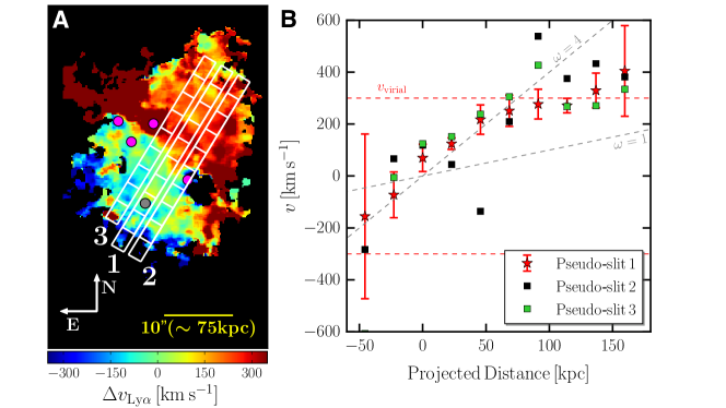
Figure 10: Ly$\alpha$ velocities along three “pseudo-slits” through the ELAN. (A) The three $2\arcsec$-wide pseudo-slits (long white rectangles) used in our analysis are overlaid on the flux-weighted velocity-shift map for the ELAN. “Pseudo-slit 1” intersects the position of the quasar SDSS J1020$+$1040 (grey circle), the peak of the ELAN at a distance of $1\arcsec$ from the quasar (at $\alpha=155.0428$ deg, $\delta=10.6679$ deg), and a secondary peak at 120 projected kpc from SDSS J1020$+$1040. Two additional pseudo-slits probe the same orientation but at symmetrically shifted positions. Each pseudo-slit is oriented at $149$ deg E from N. Along each pseudo-slit we indicate the $2\arcsec\times 3\arcsec$ boxes within which the Ly$\alpha$ centroids have been calculated (see B). The magenta circles indicate the position of the additional associated sources (Fig. 2). (B) Flux-weighted velocity shift computed along the three pseudo-slits shown in A with respect to the position and systemic redshift of SDSS J1020$+$1040. The errorbars show the uncertainty on the mean velocity $\sigma/\sqrt{S/N}$. To avoid confusion, similar errorbars are not shown for the pseudo-slits 2 and 3. The red dashed line indicates the virial velocity $v_{\rm vir}=293$ km s^-1 for a halo of $M_{\rm DM}=10^{12.5}$ M_⊙. While the grey dashed lines represent the velocity curve for solid-body rotation with $\omega=1$, or $4$ in units of $3.1\times 10^{13}$ Hz. The whole Ly$\alpha$ structure seems to show a rotation-like pattern. Analogous results are found by using Gaussian-centroided velocities (see appendix C).

Within each pseudo-slit the nebula shows small flux-weighted velocity shifts at small projected distances, and up to $300-400$ km s^-1 shifts at $160$ projected kpc. The velocity shift at large projected distances is remarkably similar to the expected virial velocity ($293$ km s^-1) of the dark matter haloes that host $z\sim 3$ quasars ($M_{\rm DM}\sim 10^{12.5}M_{\odot}$, White et al. 2012). Outlying points along each velocity curve are due to substructures in the giant nebula, like the gas associated with the faint QSO2 along “Pseudo-slit 2”. Overplotted on the figure are predictions (dashed lines) for a sphere in solid body rotation centred on the ELAN and with its angular momentum axis oriented perpendicular to the pseudo-slits. The data-points flatten out at large radii and thus do not follow such simplified models.

Secondly, to fully support our analysis using pseudo-slits, in Fig. 11 we show a two-dimensional spectrum obtained by collapsing the final MUSE datacube (PSF and continuum subtracted) along the direction of “Pseudo-slit 1”. In particular, panel A and B of Fig. 11 report the two-dimensional spectrum for the whole spatial range comprehending the ELAN (i.e. like a pseudo-slit with width of $\approx 21\arcsec$). In these panels is visible the contribution of the associated compact sources (QSO2, LAE1, LAE2, and AGN1) to the Ly$\alpha$ emission. At positive distances their intrinsic Ly$\alpha$ emission hides the signature of the rotation-like pattern on halo scales, but at negative distances the shear is visible. On the other hand, the shear at positive distances is evident when excluding these sources from the extracted two-dimensional spectrum. Indeed, panel C of Fig. 11 shows the two-dimensional spectrum extracted within “Pseudo-slit 1” together with the data-points presented in Fig. 10 (first moment of the flux distribution). The velocity shear of the diffuse Ly$\alpha$ emission extending from negative to positive distances is now clearly visible. Note that we change the flux scale between panel A and B to allow a comparison with panel C.

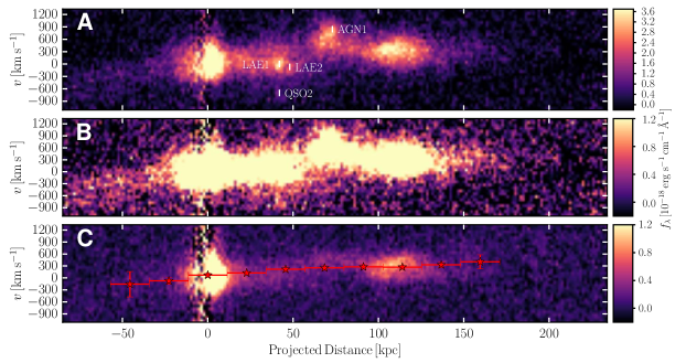
Figure 11: Two-dimensional spectrum of the ELAN along the direction of “Pseudo-slit 1”. (A) Two-dimensional spectrum of the ELAN obtained by collapsing the final MUSE datacube (PSF and continuum subtracted) along the direction of “Pseudo-slit 1” for a spatial region including the whole Ly$\alpha$ extended emission. The position for the contribution of the associated compact sources is indicated. Note that along this direction LAE1 and QSO2 are at the same projected distance from the quasar SDSS J1020$+$1040 (used here as reference). (B) same as A, but with a different flux scale (same as in panel C) to emphasise the emission at lower levels. (C) Two-dimensional spectrum of the ELAN extracted within “Pseudo-slit 1” with superimposed the data-points shown in Fig. 10. Within this pseudo-slit, the velocity pattern is not contaminated by the contribution from the compact sources, and thus clearly visible. The higher noise at 0 kpc is due to the PSF subtraction of SDSS J1020$+$1040  (see section 3.2.1).

This behaviour of a monotonically increasing velocity with increasing distance, and a flattening at larger distances, is suggestive of a “classical” galaxy rotation curve, impacted by the presence of the underlying dark matter on large scales (e.g., Persic et al. 1996). Such a large-scale rotation-like pattern is also expected in the current paradigm of galaxy formation for inspiraling material within galaxy haloes (e.g., Stewart et al. 2016). Specifically, the fraction of cool halo gas mapped in Ly$\alpha$ emission, is likely tracing the overall accretion motions within the halo, roughly centred at or near the position of SDSS J1020$+$1040. This baryonic ’rotation’ is in turn predicted to trace the motions of the underlying dark-matter.

To further explore this possibility, we compare our observations with a cosmological zoom-in simulation centred on a dark-matter halo of mass $M_{\rm DM}=10^{12.29}M_{\odot}$ at $z\approx 3$ (Wang et al. 2015, see appendix D for details on the selection of the halo) close to the masses estimated for quasar host haloes (White et al. 2012; Fanidakis et al. 2013). In particular, as the observed Ly$\alpha$ emission traces cool gas ($T\sim 10^{4}$ K) (e.g., Hennawi et al. 2015), we directly compare the observed velocity shear with the velocity patterns of the cool gas ($T<10^{4.5}$ K) in our cosmological zoom-in simulation (see appendix D for details on this temperature cut). Intriguingly, it is easy to find views of the simulated halo for which the velocity shear is similar to what is seen in our data. Fig. 12 shows mass-weighted line-of-sight velocity maps of the dark matter (panel A) and the cool gas (panel B) in our simulation. These maps are constructed for a direction perpendicular to the angular momentum axis of the cool gas in a $400$ kpc box centred on the minimum of the halo potential (appendix D). Although the dark matter and the cool gas show similar shears of the order of hundreds km/s, the dark matter lags behind the baryons which are inspiraling.

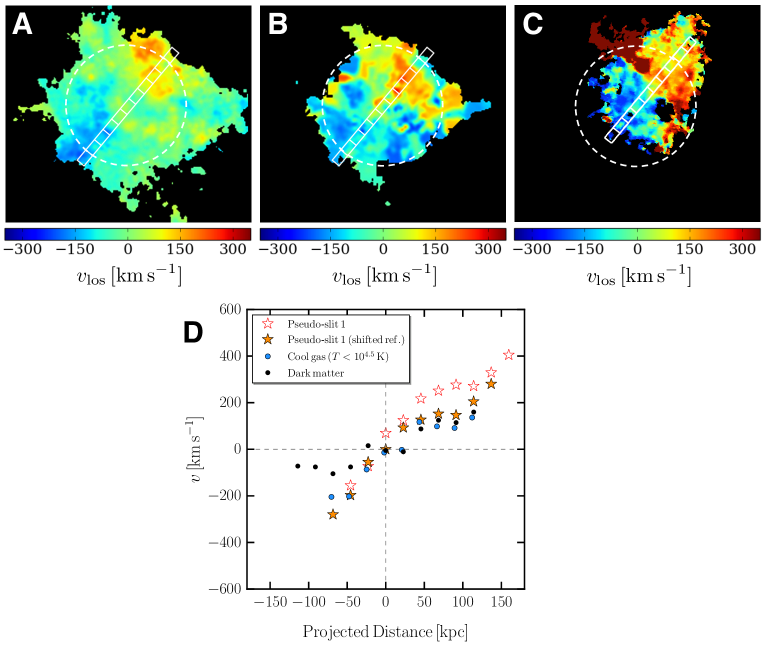
Figure 12: Comparison of the observed Ly$\alpha$ velocity pattern with the prediction of a particular direction to a simulated halo. Line-of-sight mass-weighted velocity map for (A) the dark matter and (B) the cool gas ($T<10^{4.5}$ K) in our simulation (Wang et al. 2015, appendix D), smoothed to the same resolution of the observations. The maps show the halo as seen along a direction perpendicular to the net angular momentum of the cool gas (appendix D). In both maps, the white rectangle indicates the pseudo-slit used to extract the velocity curves presented in D. The circles denote the virial radius of the simulated dark matter halo, $R_{200}=[3M_{\rm halo}/(800\pi\rho_{\rm crit}(z))]=101$ kpc. (C) flux-weighted velocity-shift map of the ELAN adapted from Fig. 6, now shown with respect to the shifted position (see D). (D) Simulated mass-weighted velocity shift computed along the pseudo-slit shown in A and B. The cool gas (blue) and dark matter (black) are compared to the flux-weighted velocity shift along “Pseudo-slit 1” (red) as from Fig. 10. In orange we show the data-points for “Pseudo-slit 1” as if the halo centre was not co-spatial with the quasar SDSS J1020$+$1040, but shifted by $\approx 23$ kpc (or $\approx 3\arcsec$) along “Pseudo-slit 1” and by $\approx-125$ km s^-1 (i.e. next white box along “Pseudo-slit 1” from the quasar position in Fig. 10), as shown in panel C. This position is also displaced from the peak of the extended Ly$\alpha$ emission at $1\arcsec$ from SDSS J1020$+$1040. To avoid confusion we omit the errorbars. Note that the errors on the simulated data-points are much smaller than the uncertainty shown for our observations in Fig. 10.

The similarity between our data (panel C in Fig. 12) and the shear present within the simulated gas can be better quantified by extracting the velocity curve along a pseudo-slit, analogous to what was done with the observations. In particular, we select the pseudo-slit that passes through the centre of the halo and best probes the velocity shear of the cool halo gas as seen in this orientation (appendix D). The bottom panel of Fig. 12 illustrates that the observed velocity shear (red points) agrees, within the uncertainties, with the simulated cool gas velocity shear (blue points) at small and negative projected distances. However, the simulation seems to under-predict the line-of-sight velocities at large positive projected distances. This can be explained by the fact that at smaller radial distances from the centre, the halo potential should dominate the kinematics, whereas halo gas at large radii (large projected distances) is expected to be more influenced by the particular large scale configuration (e.g. mergers, filaments) at a given time (e.g. More et al. 2015). Variations of the signal on $100$ kpc scales are thus expected in a halo to halo comparison. In addition, the quasar SDSS J1020$+$1040 could sit in a more massive DM halo than selected here. Such a halo would be characterised by higher circular velocity. Further, we caution that the comparison between observations and simulations suffers from the uncertainty on firmly placing the centre of the halo in observations (see section 4.1.1). Indeed, the agreement between observations and the simulation would be improved by shifting the reference position for the observed data (previously placed at SDSS J1020$+$1040) towards the companion Ly$\alpha$ emitters and the Ly$\alpha$ nebula by $\approx 23$ kpc (or $\approx 3\arcsec$) and by $-125$ km s^-1, i.e. by one box along “Pseudo-slit 1” (orange points in Fig. 12). Such a better agreement would imply that the centre of mass of the system is not precisely located at the position of SDSS J1020$+$1040.

We further test this scenario by selecting all the orientations of the simulated halo which show a clear rotation-like signal within the virial radius, and compute the velocity curves as done for the previous orientation. Specifically, we have generated hundred velocity maps for the cool halo gas by sampling the whole sphere. $\sim 20$% of this maps show a clear rotation-like signal within the virial radius. We have then extracted the velocity curves within a pseudo-slit as done previously. In Fig. 13 we compare the region spanned by these simulated velocity curves drawn from different orientations with our observations, for both the data-points estimated using the quasar as reference (red) and the shifted reference position (orange, as in Fig. 12). The good agreement between the observed and the simulated velocity curves confirms the plausibility of our interpretation, namely that the nebular Ly$\alpha$ emission traces motions of inspiraling baryons within the halo hosting the quasar SDSS J1020$+$1040. It is important to note that such motions can be easily probed by observations only if the bright Ly$\alpha$ emission extend out to large distances (comparable with the halo scale) from the quasar.

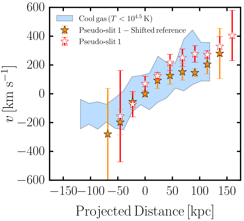
Figure 13: Comparison of the observed Ly$\alpha$ velocity pattern with the overall prediction of a cosmological zoom-in simulation of galaxy formation. The data points (red and orange) are the same as in Fig. 12. The blue shaded area indicates the region covered by the predicted velocity curves for directions to the simulated halo which show a clear rotation-like signal within the virial radius. Such directions corresponds to $\sim 20$% of the possible orientations. Given the remarkable agreement, our data seems to reveal structure assembly onto a massive dark matter halo.

4.1.1 The Position of the Centre of the Main Halo

As discussed in the previous section, our interpretation of the velocity pattern as the signature of inspiraling structures within the quasar’s halo requires the centre of the dark-matter halo to be in close proximity to SDSS J1020$+$1040. This hypothesis is supported by several pieces of evidence. First of all, clustering studies place SDSS quasars at these redshifts in very massive dark matter haloes $M_{\rm halo}\approx 10^{12.5}\,M_{\odot}$ (White et al. 2012), at least $30\times$ more massive than the haloes hosting LAEs at the same redshift, $M_{\rm halo}=10^{11\pm 1}M_{\odot}$ (e.g., Ouchi et al. 2010). Also, bright quasars at $z=2.7$ seem to sit in $M_{\rm halo}=10^{12.3\pm 0.5}\,M_{\odot}$ and to reside in groups of galaxies (Trainor & Steidel 2012). In addition, the two-point correlation function of quasars (combining SDSS DR7 quasars and the sample in Hennawi et al. 2006) requires only a very small fraction of quasars to be satellites ($f_{\rm sat}\sim 10^{-4}$ at $z=1.4$) to explain their small-scale clustering, when interpreted in the framework of the halo occupation distribution (Richardson et al. 2012). It is thus plausible that the halo of SDSS J1020$+$1040 acts as the main halo in its overdense environment, with the fainter objects being interacting structures or satellites. Intriguingly, note that the most favoured position of the centre of mass from the comparison with the direction perpendicular to the net angular momentum of the cool gas in the simulation (Fig. 12) would place the two companions AGN, QSO2 and AGN1, at symmetric velocity shift, i.e. $-701\pm 450$ km s^-1 and $739\pm 72$ km s^-1 respectively. Keeping in mind the uncertainties on the redshift determination for the two QSOs, these shifts could then reflect the peculiar velocities of the two AGN with respect to SDSS J1020$+$1040 within a massive structure.

Secondly, the Ly$\alpha$ nebula is clearly associated with SDSS J1020$+$1040, being at its systemic redshift and showing its maximum near the quasar position (at $\approx 1\arcsec$, Fig. 6). It is indeed plausible that the Ly$\alpha$ emission shows its maximum in proximity of the quasar where higher densities are expected. For example, the existence of a density profile within CGM with higher densities near the central galaxy has been proposed by Stern et al. (2016), and inferred with the absorption technique in Lau et al. (2016).

Even though the aforementioned hints are compelling, a firm determination of the halo centre would require challenging observations. Indeed, an additional evidence could be obtained by conducting a deep spectral-imaging survey (e.g. deeper IFU observations, submm data to estimate the redshift of faint or obscured companions) to characterise the velocity distribution of galaxies around SDSS J1020$+$1040. If such a distribution clearly peaks around the quasar’s systemic redshift and no comparable massive galaxies are found, SDSS J1020$+$1040 would then be considered as dominant. Obvious to say, this approach would need a statistical sample of satellites to accurately compute a velocity distribution. In addition to this approach, if SDSS J1020$+$1040 is indeed at the centre of a massive group, very deep X-ray observations might be able to constrain the emission from the diffuse hot-phase. If the peak of such emission (after removal of the intrinsic quasar’s X-rays) appears to be close to SDSS J1020$+$1040 our hypothesis would then be definitely strengthened.

Our overall approach reflects the techniques used at low redshift to constrain the properties of galaxy clusters, where the most massive galaxy has been often used as the centre of mass when other information were still not available (e.g., Kent & Gunn 1982). Finally, note that a shift of the brightest object of a group from the centre of the mass distribution is frequently seen at low redshift. For example, the brightest cluster galaxy (BCG) in the prototypical strongly lensed massive clusters A383 ($z=0.1887$) is displaced from the cluster centre by tens of kpc ($21\pm 56$ kpc) and tens of km s^-1 ($-11\pm 110$ km s^-1) (Geller et al. 2014).

4.2 Alternate Scenarios for the Observed Velocity Shear within the ELAN

In the previous section, we argue that the velocity shear within the ELAN most likely traces the kinematics of the cool gas, which is expected to show a rotation-like pattern while accreting onto a dark matter halo, as shown in current structure-formation theories and cosmological simulations. The velocity offsets detected within the gaseous structure and the association of three AGN with the ELAN, together with their large velocity offsets from SDSS J1020$+$1040, thus seems to reflect the gravitational motions within a massive structure (e.g., Miley et al. 2006; Hennawi et al. 2015). However, so far, we have neglected other possible mechanisms that might have shaped the Ly$\alpha$ emission around SDSS J1020$+$1040 (e.g., resonant scattering of Ly$\alpha$ photons).

In the next sections we thus discuss the alternate scenarios that could reproduce the observed velocity shear, which we conclude seems disfavoured given the current data. However, we emphasise that only future follow-up observations compared against future zoom-in cosmological simulations would be able to definitively rule out some of these scenarios.

4.2.1 Resonant Scattering within the ELAN

The resonant nature of the Ly$\alpha$ transition makes challenging, in most of the cases, its use as a tracer of the kinematics in astrophysical observations (e.g., Neufeld 1990, and references thereafter). In particular, a Ly$\alpha$ photon typically experiences several scatterings before escaping the system in which it is produced because of the high opacity at line centre. As Ly$\alpha$ photons must diffuse into the wings of the line to leave the system (e.g., Neufeld 1990; Cantalupo et al. 2005), double-peaked emission line profiles are thus expected especially for high neutral hydrogen column densities. In addition, because of the high number of scatterings, the emergent Ly$\alpha$ line profile could be also affected by the amount of dust and its particular distribution within the system (e.g., Neufeld 1990; Duval et al. 2014). Further, infalling or outflowing gas on galaxy scales have been shown to imprint a distinctive feature to the Ly$\alpha$ line profile, with absorption of the red or blue side of the line, respectively (e.g., Verhamme et al. 2006). Therefore, the line profile is not expected to follow a simple analytical function, and additional non-resonant diagnostics are usually required to firmly characterise the motions within a system (e.g., Yang et al. 2014; Prescott et al. 2015a). Notwithstanding these challenges, the Ly$\alpha$ line is the brightest and, in most of the cases, the only detected emission from the diffuse CGM and IGM, and hence it provides a unique opportunity to study the kinematics of these diffuse gas phases on very large scales, once the resonant scattering effects are taken into account.

Not being able to rely on non-resonant emission lines (He ii is not detected, section 3.2.2), to assess the importance of resonant scattering of Ly$\alpha$ photons within the ELAN here studied, we have thus carefully inspected the Ly$\alpha$ line shape. First, our test in appendix C.2 shows that the moment analysis presented in section 3.2.1 is in complete agreement with a Gaussian fit for all the extent of the ELAN, resulting in fully compatible maps (Fig. 21). This agreement has been further demonstrated in Fig. 22 for the emission within “Pseudo-slit 1”. As an additional check, in Fig. 14 we show the Ly$\alpha$ emission line shape in four circular regions of radius $2\arcsec$. We choose these regions because they are representative of the different velocity dispersions that are present in Fig. 6, spanning more quiescent (Region 1 and 4) and active (Region 2 and 3) portions, while covering the range of distances from SDSS J1020$+$1040 within the ELAN. Indeed, from Fig. 14 it is clear that all regions show in first approximation Gaussian lines (detected at high significance), with regions 2 and 3 presenting wider emission (FWHM$\approx 1000$ km s^-1), while regions 1 and 4 more quiescent kinematics (FWHM$\lesssim 600$ km s^-1). Therefore, we conclude that our data are well approximated by a Gaussian down to the MUSE spectral resolution of FWHM$\approx 2.83$Å, or $\approx 170$ km s^-1 at 5000Å (i.e. close to the Ly$\alpha$ line wavelength). Further, it is interesting to note that the estimate for the overall widths within the Ly$\alpha$ structure are comparable to the velocity widths observed in absorption in the CGM surrounding $z\sim 2$ quasars ($\Delta v\approx 500$ km s^-1; Prochaska & Hennawi 2009; Lau et al. 2016). Both the emission and absorption kinematics are comparable to the virial velocity $\sim 300$ km s^-1 of the massive dark matter haloes hosting quasars (M${}_{\rm DM}\sim 10^{12.5}$ M_⊙; White et al. 2012).

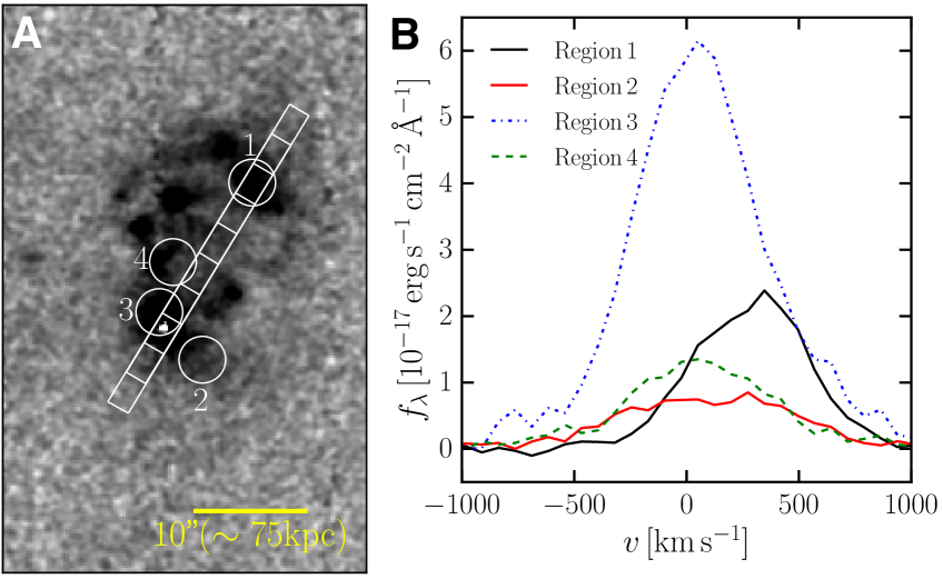
Figure 14: Ly$\alpha$ emission-line shapes for four representative regions within the ELAN. (A) NB image of the Ly$\alpha$ nebula around SDSS J1020$+$1040 after PSF subtraction. The position of 4 regions (circles with $2\arcsec$ radius) and of the slit used in Fig. 10 are shown for comparison. (B) Ly$\alpha$ line spectra of the nebula extracted within the region shown in the left panel. Note that at the resolution of our observations (FWHM $\approx 170$ km s^-1 at 5000Å), there is no evidence for double peak profiles expected for resonantly trapped Ly$\alpha$ emission. Note also the velocity shift of $\approx 300$ km s^-1 from the quasar systemic redshift for Region 1, as expected from our analysis.

All these evidences suggest that resonant scattering of Ly$\alpha$ photons do not play an important role in this system as opposed to intrinsic motions. Even though resonant scattering effects could be in place on small scales ($10$ kpc) and be hidden at the current spectral resolution (Verhamme et al. 2012) (e.g., “double-peaked” profiles, and/or faint absorption from low column density gas), we argue that on the much larger scales spanned by the Ly$\alpha$ nebula, resonant scattering seems to be negligible. Indeed, it has been demonstrated that the resonant scattering process results in a very efficient diffusion in velocity space, such that the vast majority of resonantly scattered photons produced at a certain location should escape the system after propagating for only small distances ($\lesssim 10$ kpc; Dijkstra et al. 2006; Verhamme et al. 2006; Cantalupo et al. 2014). Interestingly, to our knowledge, in all the currently known large-scale radio-quiet Ly$\alpha$ nebulosities where both Ly$\alpha$ emission and the non-resonant HeII emission are detected on $>50$ kpc scales (Prescott et al. 2015a; Cai et al. 2017), the two lines show the same shapes, suggesting that the Ly$\alpha$ line on such large scales (hundreds of kpc) might trace the kinematics of the gas just as well. For these reasons we thus claim that the extended Ly$\alpha$ emission around the quasar SDSS J1020$+$1040 can be used to trace the cool gas motions on halo scales. Further, for the same reasons, we argue that resonant scattering effects are not able to produce the $\approx 300$ km s^-1 coherent velocity shear observed within the ELAN on hundreds of kpc. However, future observations through additional diagnostics (e.g. polarization, higher resolution spectroscopy) are needed to firmly confirm the low importance of scattering within this system.

4.2.2 Two Independent “Blobs” at Two Different Redshifts within a Large-scale Structure in Projection

A first look at the velocity map in Fig. 6 could give the impression of two independent nebulae with different redshifts, i.e. one at the redshift of the quasar SDSS J1020$+$1040 and the other in the NW direction at $\approx 300$ km s^-1 (or $\Delta z\approx 0.004$), separated at the “boundary”. The velocity shift between the two nebulae could be interpreted as a large-scale structure in projection with a maximum extent of at least $600$ kpc (or a comoving distance of $\approx 2.53\,h^{-1}$ Mpc), when converting the velocity difference into distance assuming the structure to be in the Hubble flow. If this is indeed the case, to our knowledge, this structure could then represent the largest cosmic-web patch traced in Ly$\alpha$ to date. Even though we consider such a scenario of great interest, as we explicitly conduct our surveys (Arrigoni Battaia et al. 2016 and QSO MUSEUM, Arrigoni Battaia et al., in prep.) to search for large-scale structures with the hope of directly detect the IGM, we argue that several lines of evidence contradict this interpretation. We list them in what follows.
1) The peak of the Ly$\alpha$ emission continuously shifts in velocity with distance from the quasar SDSS J1020$+$1040 (Fig. 10, Fig. 11) and does not show any evidence for double-peaked Ly$\alpha$ line profiles at the “boundary”. In other words, the line profiles do not show two distinct peaks separated by $300$ km s^-1 (and thus at two different redshfits), which would be clearly distinguishable at the MUSE spectral resolution and because of the small width of the Ly$\alpha$ line within the ELAN. This can be once again appreciated in Fig. 15 where we show the Ly$\alpha$ profiles in three boxes of $2\arcsec\times 3\arcsec$ at this location (the “boundary”), which one might assume to be the region where the two nebulae overlap. In all the apertures, the Ly$\alpha$ line is characterised by a single peak slightly redshifted from the quasar systemic, as expected from our overall analysis. As also demonstrated by the Gaussian fit analysis (appendix C.2), the same exercise do not reveal any double-peaked Ly$\alpha$ profile in any region within the ELAN. If what we see are two independent nebulosities, the bright emission from these two structures thus do not overlap, but has to stop exactly where they touch in projection.
2) In the framework of two independent nebulosities, it would be difficult to explain the symmetrical gradual shift in velocities at both positive and negative projected distances ($-50<d<50$ kpc) from the quasar SDSS J1020$+$1040 (Fig. 10, Fig. 11), and justify at the same time a separation of these signatures with respect to the coherent redshifted NW portion at higher positive distances without involving any kinematics (e.g. rotation-like and accretion).
3) In a two nebulae scenario, projection effects due to our vantage point conspire to perfectly mimic the expected kinematics and sizes of a dark matter halo hosting quasars. Indeed, it is intriguing that the Ly$\alpha$ emission is detected only within $\approx 170$ projected kpc and with velocity shifts $<400$ km s^-1, when the expected virial radius for a quasar is $\approx 160$ kpc (Prochaska et al. 2014) and the expected virial velocity is $v_{\rm vir}=293$ km s^-1 ($M_{\rm DM}=10^{12.5}$ M_⊙ White et al. 2012). Such mimicking seems highly improbable for at least two reasons. First, the observed velocities along the line-of-sight within a large-scale structure in projection would be greatly affected by the flow velocities of the gas within the structure itself. Indeed the gas within filaments in haloes is expected to flow with velocities $\sim 200$ km s^-1 (Dekel et al. 2009; Goerdt & Ceverino 2015). On top of this, resonant scattering effects of Ly$\alpha$ photons may greatly affect any such structure aligned along the line-of-sight, as Ly$\alpha$ photons have to pass through the structure itself to reach the observer. Distance information would therefore be highly distorted, especially for such a large reservoir of neutral hydrogen.
4) If the structure is along the line of sight, the hard ionizing radiation of the quasar SDSS J1020$+$1040 has to impinge on the gas. Indeed, in accord with unified models of AGN (e.g. Antonucci 1993) quasars should emit in roughly symmetrical ionization cones. Being un-obscured along our line-of-sight, one should expect the quasar to be un-obscured also in the opposite direction. If this is the case, given the high luminosity of SDSS J1020$+$1040, photoionization would be undoubtedly the main powering mechanism for the whole extended emission (Cantalupo et al. 2014; Hennawi et al. 2015; Arrigoni Battaia et al. 2015b). In this scenario, the observed high Ly$\alpha$ surface brightness and the absence of extended He ii require implausibly high densities ($n_{\rm H}>100$ cm^-3) within at least $350$ kpc spanned by the ELAN in the Hubble flow. Such high density values would be in stark contrast with current cosmological simulations which predict $n_{\rm H}\sim 10^{-2}-10^{-5}$ cm^-3 in the CGM and IGM (e.g. Rosdahl & Blaizot 2012). On top of this, a photoionization scenario would predict a smooth transition between optically thin and thick gas (to ionizing radiation) while moving from small to large distances from the quasar. As the Ly$\alpha$ surface brightness is proportional to $n_{\rm H}$, and column density $N_{\rm H}$ in the optically thin regime (i.e. SB${}_{\rm Lya}^{\rm thin}\propto n_{\rm H}N_{\rm H}$), while only to the ionizing luminosity in the optically thick regime (i.e. SB${}_{\rm Lya}^{\rm thick}\propto L_{\rm\nu}$) (Hennawi & Prochaska 2013), this scenario would imply a tuning between the different values so that the transition happens while roughly preserving the same level of observed Ly$\alpha$ surface brightness in the whole extent of the ELAN (Fig. 6). We discuss this analysis in detail in appendix E.

Notwithstanding these arguments, additional observations are needed to completely rule out this scenario, i.e. polarization study of the Ly$\alpha$ emission (determination of the powering mechanism), observations in other gas tracers to confirm the Ly$\alpha$ line shape (e.g. deeper MUSE observations, deep observations targeting the H$\alpha$ line), or observations with a higher spectral resolution (importance of scattering).

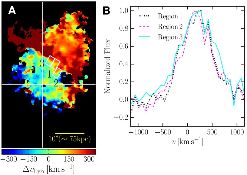
Figure 15: Ly$\alpha$ line shape at the “boundary”. (A) The three $2\arcsec\times 3\arcsec$ boxes within which the Ly$\alpha$ spectra have been extracted are overlaid on the flux-weighted centroid map for the Ly$\alpha$ emission of the giant nebula (panel B of Fig. 6). The large white cross indicates the position of the quasar SDSS J1020$+$1040 before PSF subtraction. (B) Ly$\alpha$ emission-line within the three regions shown in panel A. In each region, the Ly$\alpha$ line do not show two distinctive peaks at two different redshifts (at $0$ and $300$ km s^-1) expected in the case of two independent structures in projection. Note however, that there is a fainter and very narrow peak at $\approx 420$ km s^-1 in all of the spectra. Higher resolution data are needed to study the nature of this feature.

4.2.3 A Large Rotating Disc

A large rotating disc (in a dark-matter halo with $R=225$ kpc, $M_{\rm halo}=10^{13.1}M_{\odot}$, circular velocity $v_{\rm c}=500$ km s^-1) has been proposed to interpret the ELAN around the radio-quiet quasar UM 287 (Martin et al. 2015). We thus discuss the same scenario for our observations, even though we consider the presence of an ordered disc extremely implausible given (i) the presence of SDSS J1020$+$1040 and two strong LAEs at the same redshift and embedded within the ELAN, and (ii) the morphology of the nebula, in which there are clear substructures. Indeed a disc – unlike accreting substructures from different directions – is a coherent structure flattened on one plane and supported by rotation in the same plane. Hence, in the case of a disc, one would expect the largest and smallest velocity shifts along the major axis (the pseudo-slit direction in our case), while the velocity should drop to zero as we go from the major to minor axis.

In such a scenario, the disc centre must be placed at the “boundary” (see Fig. 6). If one assumes the disc is sitting in a massive halo like in Martin et al. (2015), circular velocities as high as 400 km s^-1 are expected at about 60 kpc. Given that the observed maximum velocity shift from the boundary is $\approx 150$ km s^-1, an almost face-on disc would be required with an inclination $i<20^{\circ}$. Indeed, the observed line-of-sight velocity within the Ly$\alpha$ “disc” would depend on the inclination of the disc itself with a $\sin\,i$ term. The morphology of the Ly$\alpha$ emission and the presence of the embedded sources run counter to this interpretation. On the other hand, if we assume an almost edge-on Ly$\alpha$ disc, the observed velocities would imply the presence of a less massive system $M\approx 10^{11.32}M_{\odot}$, in strong contrast with the predicted average mass for quasar haloes (White et al. 2012). In addition, once again, it seems implausible that the Ly$\alpha$ morphology is associated to a stable edge-on disc (see also Fig. 11).

4.2.4 A Large-scale Outflow Driven by Quasar or Star-formation Activity

Cosmological simulations of galaxy formation usually invoke the presence of AGN feedback to reproduce the observed properties of massive systems, in particular to not over-predict the stellar mass, (e.g., Sijacki et al. 2007; Schaye et al. 2015). This is because in principle supermassive black-holes (SMBHs) have enough energy to be coupled with the surrounding gas in a strong wind with velocities grater then the escape velocity of even the most massive galaxies (Silk & Rees 1998). SMBHs should thus quench star-formation by disrupting the gas reservoir within galaxies. In addition, star-formation driven winds are expected to shape the galaxy properties especially at the low mass end of the galaxy population, where the injected supernovae energy is large enough to overcome the galaxy potential (e.g., Dekel & Silk 1986; Scannapieco et al. 2008). Both these feedback mechanisms are predicted to heavily affect the gas distribution and properties on hundred kpc scales, especially when implementations with a strong coupling are used (e.g., Vogelsberger et al. 2014). Such outflows would result in high velocity shifts and velocity dispersions clearly observable with current instrumentations. We here compare our data with such a scenario. However, given the large uncertainties on the current feedback implementations and modelling of outflows, we prefer to compare our observations with current data in the literature.

The great effort in searching for AGN or star-formation driven outflows (or winds) has so far resulted in evidence for their presence on maximum ten kpc scales for radio-quiet objects at both low and intermediate redshifts (e.g., Nesvadba et al. 2011; Harrison et al. 2014; Kakkad et al. 2016; Steidel et al. 2010; Rubin et al. 2014). Hundreds kpc outflows have only been reported around HzRGs, where a strong radio-jet is able to displace the surrounding gas (e.g., Swinbank et al. 2015). In general, on kpc scales star-formation driven winds show lower peak velocities and velocity dispersions ($\sim 300$ km s^-1) than AGN powered outflows ($\sim 2000$ km s^-1). Importantly, even some of the most luminous galaxies at high redshift, such as the Ultraluminous Infrared Galaxies (ULIRG), show outflows in the ionized phase only out to few kpc ($\lesssim 15$ kpc) and with velocity up to $\sim 1000$ km s^-1 (e.g. Harrison et al. 2012), with faster outflows likely powered in the presence of an AGN. On the other hand, the large scale (hundreds of kpc) outflows around HzRGs present velocity shifts and FWHM of $>1000$ km s^-1. These outflows are often aligned with the radio axis and represent the highest surface brightness part of the extended Ly$\alpha$ emission around HzRGs (Villar-Martín et al. 2003).

This large body of observations are clearly at odds with our dataset. Indeed, given that all the embedded sources lack evidence for large displacements of the Ly$\alpha$ line peak, the relatively quiescent and continuously rising kinematics traced by the Ly$\alpha$ line around SDSS J1020$+$1040  can not be easily reconciled with an AGN wind scenario. The system around SDSS J1020$+$1040 is thus substantially different from the ELAN studied in Cai et al. (2017), and currently interpreted as powered by an obscured QSO. Indeed, in that system, two velocity components are observed with a velocity shift of $\approx 700$ km s^-1 on $\gtrsim 30$ kpc scales in both Ly$\alpha$, HeII and CIV, all presenting FWHM $\approx 700-1000$ km s^-1. The presence of these additional emission lines besides Ly$\alpha$ clearly invoke the presence of a fast shock or an embedded hard ionizing source.

Further, the large size of the ELAN around SDSS J1020$+$1040 together with the small velocity dispersion throughout its extent with a continuous peak displacement (an ordered flow pattern), seems to disfavour a star-formation-driven wind. Indeed such a scenario would require a coherent high energy input from several coeval supernovae to sustain a massive wind for hundreds of kpc within a massive system. Even though supernova driven superwinds (with velocities up to 1000 km s^-1) have been theorized to explain radio-quiet giant Ly$\alpha$ nebulae (e.g. Taniguchi & Shioya 2000), a growing body of observations are in stark contrast with such a scenario (e.g. Yang et al. 2014). In addition, even a shock with low velocities ($\sim 100$ km s^-1) may result in the production of hard ionizing photons and thus in detectable extended emission in the He ii and C iv lines within our sensitivity limits (Allen et al. 2008; Arrigoni Battaia et al. 2015a). Our upper limits on C iv/Ly$\alpha$ and He ii/Ly$\alpha$  (section 3.2.2) appear to be in contrast with the ratios expected (Figure 13 in Arrigoni Battaia et al. 2015a), and thus disfavour such a scenario. However, while we argue against a wind scenario to reproduce the velocity shear on hundreds of kpc, we cannot exclude the presence of both feedback effects on small scales (as usually reported in the literature) in close proximity to the compact sources embedded within the ELAN.

Finally, we stress the similarity of the kinematics traced within this ELAN around SDSS J1020$+$1040 with the quiescent haloes observed around HzRGs (e.g., Villar-Martín et al. 2003). Indeed, HzRGs not only present highly disturbed kinematics, but also the presence of low surface brightness haloes with velocity shifts and FWHM of few hundreds of km s^-1. This emission is usually interpreted to be associated with the cool reservoir within a quiescent host halo not perturbed by the radio activity of the HzRG (Villar-Martín et al. 2003).

4.3 Powering Mechanisms and Physical Properties of the Emitting Gas

Our observations reveal emission from only the Ly$\alpha$ transition from the ELAN associated with the quasar SDSS J1020$+$1040. Because several mechanisms could in principle act together to produce Ly$\alpha$ emission on hundreds of kpc scales (section 3.2.2), characterizing the physical properties of the emitting gas is a problem of complexity, and only ad-hoc comprehensive simulations of massive haloes would shed light on the nature of bright and giant Ly$\alpha$ nebulae, once the current computational problems would be bypassed (e.g. Cantalupo et al. 2014; Arrigoni Battaia et al. 2015a; Hennawi et al. 2015; McCourt et al. 2016 and appendix D). Here we briefly discuss which mechanisms could be in play, and what physical properties are then expected.

The dominant powering mechanism has to reproduce the high level of the observed surface brightness of the Ly$\alpha$ line SB${{}_{\rm Ly\alpha}\sim 10^{-17}\,{\rm\,erg\,s^{-1}\,cm^{-2}\,arcsec^{-2}}}$ on scales of $\sim 100$ kpc, together with its kinematics. Specifically, the ELAN around SDSS J1020$+$1040 shows overall quiescent kinematics (FWHM$\lesssim 600$ km s^-1), with more disturbed and active ones (larger velocity dispersion) in proximity of the three AGN, and a rotation-like pattern.

Such quiescent kinematics has been seen in several extended Ly$\alpha$ nebulae discovered so far around radio-quiet quasars for which we have spectroscopic information (Martin et al. 2014; Hennawi et al. 2015; Borisova et al. 2016). All these nebulosities have been overall interpreted as powered by fluorescence emission, i.e. recombination radiation boosted by the quasar ionizing radiation (e.g., Cantalupo et al. 2005; Kollmeier et al. 2010). However, if the luminous quasar does not shine directly on the surrounding gas (e.g. depending on its opening angle and orientation), then alternative powering mechanisms, i.e. photoionization from star-formation, shocks from superwinds (e.g., Taniguchi & Shioya 2000; Mori et al. 2004), scattering of Ly$\alpha$ photons (e.g.,Dijkstra & Loeb 2008), and “cooling radiation” (e.g., Haiman et al. 2000; Rosdahl & Blaizot 2012), could still be relevant. In the case of SDSS J1020$+$1040, we have already discussed the evidence against the presence of superwinds or a large contribution from resonant scattering, concluding that these processes could only be effective in altering the ELAN properties on small scales ($\lesssim 10$ kpc) (section 4.2). In the remainder of this section we briefly consider “cooling radiation” and photoionization in the case of SDSS J1020$+$1040.

4.3.1 Cooling radiation

“Cooling radiation”, i.e. collisional excitation driven Ly$\alpha$ emission from gravitational accretion, is often invoked to explain extended Ly$\alpha$ emission (e.g., Fardal et al. 2001; Rosdahl & Blaizot 2012). The strength of such emission is largely “controlled” by the collisional excitation coefficient given by ${C_{\rm Ly\alpha}=3.7\times 10^{-17}}$ ${{\rm exp}(-h\nu/k_{\rm B}T)/T^{1/2}}$ erg s^-1 cm³ (Osterbrock 1989), where $h$ is the planck constant and $k_{\rm B}$ is the Boltzmann constant. Given the exponential dependence on temperature of $C_{\rm Ly\alpha}$ and (being a collisional process) on gas density squared (in the ionized case), this mechanism requires a “fine tuning” between the temperature and density of the gas to reproduce the observed bright SB_Lyα, while taking into account the detail balance of heating and cooling within the gas itself. Dijkstra & Loeb (2009) argue, while modelling LABs in an analytical way, that if $\gtrsim 10$% of the change in gravitational binding energy in ISM-like dense ($n_{\rm H}\gtrsim 1$ cm^-3) cold ($T\sim 10^{4}$ K) flows goes into heating of the gas, then cold flows in massive haloes ($M_{\rm halo}~{}10^{12}-10^{13}$ M_⊙) would be detectable as LABs. The same picture, but with lower densities, has been reproduced with cosmological simulations (Furlanetto et al. 2005; Faucher-Giguère et al. 2010; Rosdahl & Blaizot 2012). These works show how gas with $n_{\rm H}\gtrsim 0.3$ cm^-3 (the CGM for those simulations), whose emission is dominated by collisional excitation, accounts for 40% of the total Ly$\alpha$ luminosity (Rosdahl & Blaizot 2012), and could be detected as a LAB. The high gas densities in the cold flows are caused by the confinement due to the presence of hot gas within the virial radius of the system (Dijkstra & Loeb 2009). For this reason, it is expected that outside the virial radius the emission powered by “cooling radiation” declines considerably as no hot gas is present and the cold flows would then be much more rarefied (Dijkstra & Loeb 2009; Dekel et al. 2009; Kereš et al. 2009).

One could speculate that cooling radiation is indeed what we see around SDSS J1020$+$1040. Indeed, in the favoured scenario (i.e., inspiraling cool gas), we probe the quasar halo, and therefore the Ly$\alpha$ emission does not extend much beyond the expected virial radius. In addition, the infall of the gas is expected to occur with coherent velocities of the order of $200$ km s^-1 (e.g., Dekel et al. 2009; Goerdt & Ceverino 2015), which are consistent with the observed velocity dispersion. Further, in this scenario, our non detections on large scales for the He ii and C iv lines would reflect the low signal expected in He ii in massive haloes (SB${}_{\rm HeII}\sim 10^{-20}\,{\rm\,erg\,s^{-1}\,cm^{-2}\,arcsec^{-2}}$; Yang et al. 2006), and the low metallicity expected for inflowing gas (but note Lau et al. 2016), respectively.

4.3.2 Photoionization

Even though the emission around SDSS J1020$+$1040 seems to be interpretable in light of a “cooling scenario” in the aforementioned qualitative way, the high Ly$\alpha$ surface brightnesses on hundreds of kpc scales (SB${}_{\rm Ly\alpha}\sim 10^{-17}\,{\rm\,erg\,s^{-1}\,cm^{-2}\,arcsec^{-2}}$) are not easily reproduced in simulations with current expected densities and temperatures (e.g., Rosdahl & Blaizot 2012; Faucher-Giguère et al. 2010), and it is thus difficult to firmly assess if this is the main powering mechanism. To reproduce the observed high SBs, lower temperatures or higher densities in the framework of a “pure” cooling radiation scenario are thus needed. In this regard, note that cosmological simulations could probably still miss high densities in the CGM due to computational issues or current subgrid prescriptions. Indeed, the above-mentioned works show that to reproduce the LABs, the Ly$\alpha$ emission should come from gas dense enough to be almost star-forming in their simulations (e.g., Furlanetto et al. 2005; Faucher-Giguère et al. 2010; Rosdahl & Blaizot 2012).

In addition, the sources embedded within the Ly$\alpha$ emission could photoionize the surrounding gas and thus boost the Ly$\alpha$ signal through recombination radiation (fluorescence). This effect has not been accounted for when dealing with the “cooling radiation” scenario (e.g., Dijkstra & Loeb 2009; Rosdahl & Blaizot 2012), as studies were focused on a conservative “cooling flow” framework. Given the very mild dependence on temperature and ionisation state for the recombination radiation, this process seems more plausible for extended Ly$\alpha$ nebulae around quasars (e.g., Cantalupo et al. 2014; Borisova et al. 2016). The far higher luminosity of SDSS J1020$+$1040 in comparison to its companions (see section 3.1), likely makes it the dominant source of radiation if it illuminates the ELAN. However, we don’t exclude the possibility that the type-2 AGN1 may be brighter as seen from the nebula than from our perspective. Nevertheless, it is unlikely that its emission overcame the ionizing radiation from SDSS J1020$+$1040, given the intensity of the observed narrow lines, e.g. C iv.

If we then assume the ELAN to span the CGM around SDSS J1020$+$1040, and the bright quasar to illuminate it, the emitting gas has to be highly ionized, and thus optically thin to the ionizing radiation (Arrigoni Battaia et al. 2015b). In this regime, the Ly$\alpha$ emission would follow SB${}_{\rm Ly\alpha}^{\rm thin}\propto n_{\rm H}N_{\rm H}$, and thus would not depend on the luminosity of the central source (as long as the quasar is able to keep the gas ionized) (Hennawi & Prochaska 2013). If the physical properties of the emitting gas ($n_{\rm H}$, $N_{\rm H}$) are roughly the same, the aforementioned relation thus naturally explain the roughly constant high surface brightness in the whole extent of the ELAN.

As shown by Arrigoni Battaia et al. (2015b), strong constraints on the level of the He ii line can break the degeneracy between $n_{\rm H}$ and $N_{\rm H}$ (and thus the cool gas mass) inherent in the observation of the SB_Lyα alone in this optically thin regime. We thus use the Cloudy photoionization code (v10.01), last described by Ferland et al. (2013), to constrain the physical properties of the emitting gas around the quasar SDSS J1020$+$1040, focusing in particular on the NW emission at $\approx 120$ kpc (the high S/N portion, solid red contour in Fig. 8). In particular, we perform a similar analysis as in Arrigoni Battaia et al. (2015b), using

1. their same prescriptions for the input quasar SED, using the MUSE spectrum of SDSS J1020$+$1040  (Fig. 2) and masking the Ly$\alpha$ and C iv lines to avoid contribution to both emissions from scattering of photons from the quasar. As in Arrigoni Battaia et al. (2015b), for the extreme ultraviolet (UV) we adopt a slope of $\alpha_{\rm UV}=-1.7$ (Lusso et al. 2015), and determine the luminosity at the Lyman limit of SDSS J1020$+$1040 to be $L_{\nu_{\rm LL}}=2.8\times 10^{31}$ erg s^-1;
   

2. a standard plane-parallel geometry for the emitting clouds illuminated by the quasar at a distance of $120$ kpc;
   

3. a grid of models with this wide range of parameters given the dependence of SB_Lyα on $n_{\rm H}$, and $N_{\rm H}$, and the dependence on metallicity ($Z$) of the C iv and He ii lines, and of the collisional excitation:

   1. $n_{\rm H}=10^{-2}-10^{3}$ cm^-3 (steps of 0.2 dex),

   2. $N_{\rm H}=10^{18}-10^{22}$ cm^-2 (steps of 1 dex),

   3. $Z=10^{-3}-1$ Z_solar (steps of 1 dex).

Note that photoionization models are self-similar in the ionization parameter $U\equiv\frac{\phi_{\rm LL}}{cn_{\rm H}}$, which is the ratio of the number density of ionizing photons to hydrogen atoms. As the luminosity of the quasar is known, the variation of $U$ results from the variations of $n_{\rm H}$, as can be seen in panel F of Fig. 16, where we show the predictions of this calculation for $Z=0.1$ Z_solar (expected for CGM gas; Lau et al. 2016). As we discuss in section 3.2.2, our MUSE observations constrain the Ly$\alpha$ emission of the NW bright clump at $120$ kpc to be SB${}_{\rm Ly\alpha}=(1.81\pm 0.08)\times 10^{-17}{\rm\,erg\,s^{-1}\,cm^{-2}\,arcsec^{-2}}$, and yields $5\sigma$ upper limits of SB${}_{\rm HeII}<8.1\times 10^{-19}{\rm\,erg\,s^{-1}\,cm^{-2}\,arcsec^{-2}}$ and SB${}_{\rm CIV}<7.2\times 10^{-19}{\rm\,erg\,s^{-1}\,cm^{-2}\,arcsec^{-2}}$. On the other hand, each photoionization model in our grid predicts the intensity of these emission lines. Fig. 16 report the trajectory of these models of different $N_{\rm H}$ as a function of $n_{\rm H}$ and compare those values to our measurements. Our calculation confirms that optically thin gas (log$[N_{\rm HI}/{\rm cm}^{-2}]\ll 17.2$; see panel B) can reproduce the SB_Lyα at the NW clump (horizontal line in panel A), while optically thick gas would result in $\approx 20\times$ higher levels of emission. However, it is clear that the models that reproduce the observed SB_Lyα present levels of He ii too high to be in agreement with our observations (see panels C), unless the emitting gas is characterized by very high densities and low column densities. Specifically, only models with $n_{\rm H}\gtrsim 690$ cm^-3 and ${\rm log}[N_{\rm H}/{\rm cm}^{-2}]\lesssim 18$ are able to match our observations (${\rm SB}_{\rm Ly\alpha}$ and He ii upper limit). Given the stringent constraint He ii/Ly$\alpha$$<0.045$, this result is also valid for the other metallicities here studied (see Figure 7 in Arrigoni Battaia et al. 2015b), and would change by roughly a factor of 3 ($n_{\rm H}>250$ cm^-3, Arrigoni Battaia et al. 2015b) if we adopt the softest ionizing slope ($\alpha_{\rm UV}$=-2.3) in agreement (within $1\sigma$) with the quasar average spectrum in Lusso et al. (2015). The high values for $n_{\rm H}$ and low values for $N_{\rm H}$ are in strong contrast with the average values expected within the quasar CGM, i.e. $n_{\rm H}\approx 10^{-2}-10^{-3}$ cm^-3 and log$N_{\rm H}=20.5$ (e.g., Rosdahl & Blaizot 2012; Lau et al. 2016; Arrigoni Battaia et al. 2016). This result exacerbates similar conclusions found when studying the ELAN around the quasar UM 287, i.e. $n_{\rm H}\gtrsim 3$ cm^-3 and log$N_{\rm H}\lesssim 20$ (Arrigoni Battaia et al. 2015b), and would thus increase the tension with current simulations of cosmological structure formation (see discussion in Cantalupo et al. 2014; Crighton et al. 2015; Arrigoni Battaia et al. 2015b; Hennawi et al. 2015; McCourt et al. 2016), which are currently not able to follow such high densities within the diffuse CGM/IGM. However, as the predicted values in the case of SDSS J1020$+$1040 seem implausible in comparison to the expectations, we conclude that the quasar is probably not directly shining on the ELAN, or/and it should have a spectral energy distribution much softer than the average quasar.

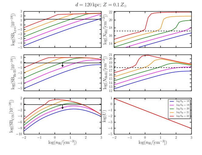
Figure 16: Photoionization modeling of the maximum within the NW redshifted emission assumed to be at $120$ kpc, $Z=0.1$ Z_⊙. The calculation has been performed using the photoionization code Cloudy (Ferland et al. 2013). We show, as a function of $n_{\rm H}$, the predicted SB_Lyα in units of $10^{-18}{\rm\,erg\,s^{-1}\,cm^{-2}\,arcsec^{-2}}$, the predicted column density of neutral hydrogen $N_{\rm HI}$, the predicted SB${}_{\rm He\,II}$ in units of $10^{-18}{\rm\,erg\,s^{-1}\,cm^{-2}\,arcsec^{-2}}$, the predicted column density of singly ionized helium $N_{\rm He\,II}$, the predicted SB${}_{\rm C\,IV}$ in units of $10^{-18}{\rm\,erg\,s^{-1}\,cm^{-2}\,arcsec^{-2}}$, and the ionization parameter $U$, respectively in (A), (B), (C), (D), (E), and (F). The solid horizontal lines show our measurement for SB_Lyα and the upper limits for SB${}_{\rm He\,II}$ and SB${}_{\rm C\,IV}$. The horizontal dashed lines indicate the theoretical threshold dividing the optically thin regime from the optically thick case for that element. For neutral hydrogen is at $N_{\rm HI}=10^{17.2}$ cm^-2, while for helium is at $N_{\rm He\,II}=10^{17.8}$ cm^-2. If the quasar SDSS J1020$+$1040 is illuminating the emitting gas, only models with $n_{\rm H}\gtrsim 690$ cm^-3 and ${\rm log}[N_{\rm H}/{\rm cm}^{-2}]\lesssim 18$ would match our observational constraints at this position.

In the case of a photoionization scenario, the fainter embedded sources together with eventual obscured sources not detected in our observations (i.e. obscured starbursts, sub-millimeter galaxies) could thus probably largely contribute to the powering of the Ly$\alpha$ emission. In particular, given the expected softer UV radiation from star-forming galaxies with respect to a quasar, photoionization from these objects could explain the observed level of SB_Lyα, together with the non-detections in He ii and C iv with more reasonable densities ($\sim 1$ cm^-3). In addition, part of the cool CGM in quasar haloes and emitting in Ly$\alpha$ could be gas stripped from infalling satellites (e.g., Arrigoni Battaia et al. 2012). Such gas has been predicted to emit preferentially through collisional excitation in low-redshift systems, though definite conclusions on this have not been reached (e.g., Tonnesen & Bryan 2011). If this is the case also at high redshift, part of the Ly$\alpha$ emission could be due to this process, and would result in larger and brighter ELANe depending on the phase of the interaction we witness. Further, powering mechanisms linked to companion objects can explain (i) the detections of the rotation-like pattern in a transverse direction with respect to the bright quasar without requiring ad-hoc orientation of the ionizing cone together with an ad-hoc wide opening angle for the AGN emission ($>90^{\circ}$), and (ii) the asymmetry of the ELAN, or in other words the absence of bright extended emission detected at negative distances from the quasar without requiring lack of cool gas within the ionizing cone of the quasar. Indeed at these locations no bright companions are detected down to our sensitivity limit.

Finally, extended star-formation may be occurring in this large-scale nebula, and thus power, at least partially, the Ly$\alpha$ emission. Indeed, the presence of widespread star-formation and molecular gas on hundreds of kiloparsecs has been unveiled in the case of the Spiderweb radio-galaxy at $z=2.161$, where a giant Ly$\alpha$ nebula encompass several galaxies (Emonts et al. 2016).

Summarizing, we can not firmly constrain the powering mechanism for the extended Ly$\alpha$ emission. Most likely, the high level of SB_Lyα that we discovered is due to a complex combination of all the aforementioned processes. Additional observations are thus needed to disentangle the contributions from each mechanism. A step towards a better understanding of this system could originate from our follow-up campaign in the submillimeter regime (to search for the presence of dust-obscured highly star-forming galaxies associated with the ELAN, e.g., Geach et al. 2016, extended star formation, and molecular gas), or by our planned observations to estimate the polarization of the Ly$\alpha$ emission (to verify the importance of scattering within the ELAN and to understand which are the powering sources, e.g. Prescott et al. 2011). Notwithstanding these uncertainties, the bright levels of Ly$\alpha$ emission seems to imply high $n_{\rm H}$ values ($\gtrsim 1$ cm^-3) irrespective of the powering mechanism invoked.

5 Summary and Conclusions

To characterise the frequency of detection of the enormous Ly$\alpha$ nebulae (ELANe) (${\rm SB}_{\rm Ly\alpha}\gtrsim 10^{-17}$erg s^-1 cm^-2 arcsec^-2 at 100 kpc) around quasars (Cantalupo et al. 2014; Hennawi et al. 2015; Cai et al. 2017), and characterise the physical properties of the CGM/IGM in emission, we have initiated a survey of the population of $z\sim 3$ quasars using MUSE on VLT, i.e. QSO MUSEUM (Arrigoni Battaia et al., in prep.). In this framework, we here report the discovery of an additional ELAN around the radio-quiet quasar SDSS J1020$+$1040 at $z=3.167$. This ELAN spans a maximum projected distance of 297 kpc, and show an average Ly$\alpha$ surface brightness ${\rm SB}_{\rm Ly\alpha}\sim 6.04\times 10^{-18}$erg s^-1 cm^-2 arcsec^-2(within the $2\sigma$ isophote). Notwithstanding the high ${\rm SB}_{\rm Ly\alpha}$, the ELAN does not show extended emission in He ii and C iv down to our deep SB limits, resulting in stringent upper limits on the line ratios, i.e. He ii/Ly$\alpha$$<0.020$ and C iv/Ly$\alpha$$<0.018$ ($5\sigma$).

Further, this ELAN is associated with an additional four embedded sources besides SDSS J1020$+$1040, i.e. two LAEs and two faint AGN SDSS J1020$+$1040 thus seems to reside in an overdense environment as the ELAN associated with the only quadruple AGN known at high redshift (Hennawi et al. 2015). Such an occurrence hints to a scenario in which ELANe are preferentially observed in overdensities (Matsuda et al. 2005, 2009; Saito et al. 2006; Prescott et al. 2008; Yang et al. 2009; Hennawi et al. 2015).

Also, this ELAN shows coherent kinematics, i.e. small gradient (300 km s^-1) and velocity dispersion ($<270$ km s^-1), on very large scales (hundreds of kpc) at high significance. Specifically, the ELAN shows a velocity shear of $\sim 300$ km s^-1 between its SE and NW edges. After considering several scenarios (e.g., resonant scattering, outflows, coherent disc) to explain this observed velocity shear, and by comparing the velocity field of the ELAN with a cosmological zoom-in simulation, we conclude that we are likely witnessing the accretion of sub-structures onto a central massive halo. Our discovery is in agreement with current theory of structure formation for infalling sub-structures which predict the presence of a rotation-like pattern on halo scales. Our interpretation thus remarkably differs from previous studies in the literature which explain the kinematics within extended Ly$\alpha$ nebulae as coherent thin discs, on similar sizes (Martin et al. 2015) or on smaller scales (radius of $\approx 3$″or $\approx 25$ kpc; Prescott et al. 2015b).

Independent of the origin for the observed cool halo gas (e.g., hot or cold mode accretion, stripping of satellite galaxies, feedback), our observations reveal the potential for high precision spatial mapping of gas kinematics on circumgalactic and intergalactic scales around massive systems, thought to be the progenitors of present-day elliptical galaxies (White et al. 2012). Such observations encode precious information about the formation of such systems, possibly unveiling clues on the intimate connection between baryons, dark matter, and the large-scale structures at these early epochs (e.g. van den Bosch et al. 2002; Sharma & Steinmetz 2005; Aragón-Calvo et al. 2007; Zhang et al. 2009; Codis et al. 2012; Zjupa & Springel 2017). Ultimately, a large sample of similar observations would enable a statistical characterisation of the geometrical uncertainties inherent to this study, and open up the possibility of comparing the angular momentum of the observed halo gas to the predicted spin of their dark matter haloes. This would allow us to better comprehend the angular momentum build-up that eventually leads to the formation of a central massive disc (Fall & Efstathiou 1980; Stewart et al. 2016), before further accretion, violent mergers and interactions reshape it into an elliptical galaxy (e.g., Gott 1975; Oser et al. 2010). Although there is a wealth of theoretical work addressing the formation of Milky Way analogs, we stress the lack of simulations targeting more massive systems ($M_{\rm DM}>10^{12}\,M_{\odot}$ at $z\approx 3$). Further development on this mass scales, with particular emphasis on the challenges in reproducing ELANe (Cantalupo et al. 2014; Arrigoni Battaia et al. 2015b; Hennawi et al. 2015; McCourt et al. 2016 and appendix D), are crucial to examine the processes of galaxy formation and gas accretion at early times. With the ongoing and planned observations with new sensitive integral-field spectrographs (e.g., Borisova et al. 2016, Arrigoni Battaia et al., in prep.) this field is rapidly emerging.

Appendix A The Systemic Redshift of the Quasar SDSS J1020$+$1040

Because of shifts between broad lines and the presence/shape of the broad lines themselves, it is notoriously difficult to obtain precise estimates of the systemic redshifts of quasars (e.g., Hewett & Wild 2010; Bolton et al. 2012; Pâris et al. 2012; Shen et al. 2016). The redshift reported in the literature for SDSS J1020$+$1040 is $z=3.1589\pm 0.0003$ (SDSS-DR12 Quasar catalogue), or previously $z=3.1678\pm 0.0008$ (Adelman-McCarthy & et al. 2009). However, the uncertainty on the redshift seems underestimated in both works, given the absence of data covering narrow emission lines. For this reason, in this study, we use as systemic redshift the estimate from the C iv line after correcting for the known luminosity-dependent blueshift of this line with respect to systemic (Richards et al. 2011; Shen et al. 2016), i.e. $z_{\rm SDSS\,J1020+1040}=3.164\pm 0.006$. Indeed, Shen et al. (2016) has shown that, according to the quasar luminosity, the redshift determined from C iv is shifted by ${v=14-122\times({\rm log}(\lambda L_{1700\textup{\AA}})-45)}$ km s^-1 (where $L_{1700\textup{\AA}}$ is the monochromatic luminosity at rest-frame 1700Å). In this formula, negative velocities indicate blueshifts from systemic, and thus a positive correction needed to get the correct systemic redshift. From the MUSE spectrum of SDSS J1020$+$1040 extracted within a circular region ($R=1.5\arcsec$; see Fig. 2), we obtain $f_{1700\textup{\AA}}=(19.4\pm 0.5)\times 10^{-17}$erg s^-1 cm^-2 Å^-1  , and thus $\lambda L_{1700\textup{\AA}}=(2.87\pm 0.07)\times 10^{46}$ erg s^-1. Using this value, we estimate an expected blueshift of -164 km s^-1. We then estimate the peak of the C iv line, as specified in Shen et al. (2016), and obtained $z=3.162$. Adding the previously determined shift gives then $z_{\rm SDSS\,J1020+1040}=3.164\pm 0.006$. The error on the redshift reflects the 415 km s^-1 intrinsic uncertainty of the empirical calibration in Shen et al. (2016). To have a firm interpretation of the system surrounding SDSS J1020$+$1040, a better determination of the redshift is certainly needed. However, we note that the narrow and bright emission evident after the PSF subtraction in close proximity to the bright quasar, which we interpret as the extended emission line regions (EELR; Husemann et al. 2014) associated with SDSS J1020$+$1040, has a redshift in agreement with the above calculation, i.e. $z=3.167\pm 0.001$ (see section 3.2). In this work, we thus assume that the quasar and the ELAN are at the same redshift, and thus physically associated.

Appendix B The Quasar SDSS J1020$+$1040  is Not Radio-Loud

As discussed in section 2, while building our survey QSO MUSEUM, we have carefully selected our targeted quasars to try to cover any dependence on the presence of an ELAN with radio activity, companion sources, luminosity, etc. Thus, we collect from the literature these information, if present, and check for any inconsistency.

In the case of SDSS J1020$+$1040, we found that it has been so far considered as the counterpart of a strong radio emission ($F=515$ mJy at 1.4 GHz; Condon et al. 1998), and thus as a radio-loud object. However, the available radio data together with our MUSE data clearly rule out an association of the quasar SDSS J1020$+$1040 with the strong radio emission, which instead appear related to an unknown HzRG at $\sim 30\arcsec$ from the quasar SDSS J1020$+$1040, but at much lower redshift.

Specifically, SDSS J1020$+$1040 was initially catalogued as counterpart of the radio emission within the Fourth Cambridge Survey (Pilkington & Scott 1965), with the name 4C 10.29, and subsequently in the Parkes survey (Ekers 1969), with the name PKS 1017+109. Also, Condon & Broderick (1985, 1986) and White & Becker (1992) reported SDSS J1020$+$1040 as the counterpart of an emission with $F=538$ mJy at 1.4 GHz. None the less, the spatial resolution of these datasets were not optimal for source matching at arcsec precision, e.g. Condon & Broderick (1985, 1986) has a resolution of $700\arcsec$.

Also the Texas Survey of Radio Sources at 365 MHz (TXS, Douglas et al. 1996) and the NRAO VLA Sky Survey at 1.4 GHz (NVSS, Condon et al. 1998), with a resolution of $5\arcsec$ and $45\arcsec$, reported the quasar as counterpart of the radio emission. This happened even though both these surveys, with a position precision estimated to be $<1\arcsec$, were able to detect the position shift of $\sim 33\arcsec$ between their reported position for the radio emission and the quasar SDSS J1020$+$1040  (see Table LABEL:tabHzRG). Probably the absence of detected optical sources at the location of the radio emission made the quasar the best alternative given the available optical catalogs at that time. Recently, data at 1.4 GHz with higher spatial resolution undoubtedly show that there is a shift of $\approx 33\arcsec$ between SDSS J1020$+$1040 and the strong radio emission (Condon et al. 1998; Becker et al. 1994).

Notwithstanding the work by Condon et al. (1998) and Becker et al. (1994), due to the former erroneous association, the quasar SDSS J1020$+$1040 has been included till now in radio-loud samples (e.g., Curran et al. 2002; Ellison et al. 2008). In particular, it is worth noting that if one follows the last edition (13th) of the catalogue by Véron-Cetty & Véron (2010), one would end up classifying SDSS J1020$+$1040 as definitely radio-loud. Indeed, the most used definition of radio-loudness requires that the ratio $R=f_{\nu,\,{\rm 5GHz}}/f_{\nu,\,{\rm 4400\textup{\AA}}}>10$ (Kellermann et al. 1989), where $f_{\nu,\,{\rm 5GHz}}$ is the 5 GHz radio rest-frame flux density, and $f_{\nu,\,{\rm 4400\textup{\AA}}}$ is the 4400Å optical rest-frame flux density. At the redshift of SDSS J1020$+$1040, one can use the information at 1.4 GHz (observed) for the radio emission, and interpolate the data for the $H$ and $K$ bands to get the optical rest-frame flux at $4400$Å. In this regard, Véron-Cetty & Véron (2010) list $F=538$ mJy at 1.4 GHz (Condon & Broderick 1985, 1986; White & Becker 1992), while the infrared information come from the Two Micron All Sky Survey (2MASS; Skrutskie et al. 2006), with a magnitude of $H=15.49$, and $K=15.32$. It is thus evident that SDSS J1020$+$1040 would be classified as radio-loud.

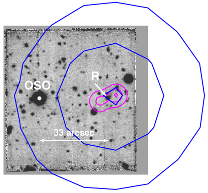
Figure 17: SDSS J1020$+$1040 is radio-quiet: discovery of an HzRG. White-light image of the combined exposures of our final MUSE datacube (as in panel A of Fig. 1) with superimposed the radio contours from the NVSS (blue; Condon et al. 1998) and VLA FIRST Survey (magenta; Becker et al. 1994) for the radio source at $\approx 30\arcsec$ from SDSS J1020$+$1040. Both sets of contours are shown at ${\rm S/N}=2$, $10$, and $20$. Owing to their higher spatial resolution ($5\arcsec$) with respect to the NVSS ($45\arcsec$), the data from the FIRST survey show two resolved structures, which we interpret as the radio lobes of a previously unknown radio galaxy. The MUSE spectrum for the optical counterpart (host galaxy) “R” of the radio emission is shown in Fig. 18, confirming this interpretation.

In Fig. 17 we show the “white-light” image from our final MUSE datacube with radio contours superimposed. Specifically, the $S/N=2$, $10$, and $20$ contours from the NVSS (blue; Condon et al. 1998), and from the VLA Faint Images of the Radio Sky at Twenty-Centimeters Survey (magenta; FIRST, resolution of $5\arcsec$, Becker et al. 1994) are indicated in blue and magenta, respectively. The shift between the quasar and the radio emission is evident, with values of $33.1\arcsec$ and $32.35\arcsec$ (average), from the NVSS and FIRST survey positions, respectively. While the superior resolution of the FIRST data reveals two bright structures separated by $7.6\arcsec$, the total integrated flux is in agreement between the two surveys (i.e. the sum of the two sources in FIRST is equal to the flux observed in the NVSS; see Table LABEL:tabHzRG).

Table 3: Summary of the radio data able to resolve the distance between SDSS J1020$+$1040 and the discovered HzRG.

Survey	RA	Dec	Separation	Flux	Reference
	(J2000)	(J2000)	(arcsec)	(Jy)
TXS	10:20:07.79	+10:40:02.8	32.6	1.642 (at 365 MHz)	Douglas et al. (1996)
NVSS	10:20:07.76	+10:40:03.5	33.1	0.515 (at 1.4 GHz)	Condon et al. (1998)
FIRST	10:20:08.05	+10:40:01.5	28.7	0.218 (at 1.4 GHz)	Becker et al. (1994)
	10:20:07.56	+10:40:04.1	36.0	0.309 (at 1.4 GHz)

Furthermore, we are able to classify this radio source. As discussed in section 2, between the program 094.A-0585(A) and 096.A-0937(A) we offset the position of SDSS J1020$+$1040 by about $15\arcsec$ to the East to try to obtain a spectrum of any optical counterpart to the radio emission. Inspection of the final MUSE datacube at the location of the two bright radio spots detected in FIRST, reveals that there are no optical counterparts down to our continuum sensitivity level (in the “white-light” image, $f_{\lambda,1\sigma}=1.1\times 10^{-21}$ erg s^-1 cm^-2 Å^-1 pixel^-1), but there is a faint source in between ($i=23.94\pm 0.02$), source “R” (Fig. 17). Given this geometric configuration we realised that this source is likely a radio galaxy, with the two radio sources being its bright radio lobes. This association is confirmed by the optical spectrum of “R” extracted from the MUSE datacube (see Fig. 18), which shows the emission lines expected in this wavelength range from a radio galaxy, i.e. C iii]$\lambda$1909, C ii]$\lambda$2327, and [Ne v]$\lambda$3426, and the characteristic red upturn of the continuum due to the sum of the contribution from the old stellar population in the host galaxy and the reddened AGN at the centre of the system (e.g., McCarthy 1993). Further confirmation is given by the agreement between the ratios of the rest-frame emission line equivalent widths for our newly discovered HzRG, EW${}_{\rm rest}^{\rm C\,III]}$/EW${}_{\rm rest}^{\rm C\,II]}=1.81\pm 0.41$ and EW${}_{\rm rest}^{\rm[Ne\,V]}$/EW${}_{\rm rest}^{\rm C\,II]}=1.51\pm 0.31$ (see Table LABEL:tabTwoHzRG), and the values reported for a composite of HzRGs presented in McCarthy (1993), EW${}_{\rm rest}^{\rm C\,III]}$/EW${}_{\rm rest}^{\rm C\,II]}=1.68$ and EW${}_{\rm rest}^{\rm[Ne\,V]}$/EW${}_{\rm rest}^{\rm C\,II]}=1.16$. In addition, the analysis of the emission-lines indicates that this newly discovered radio galaxy is at a redshift of $z=1.536\pm 0.001$ (see Table LABEL:tabTwoHzRG), and thus is not physically related to SDSS J1020$+$1040.

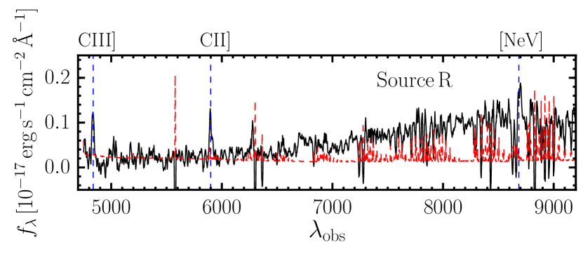
Figure 18: 1D spectrum for the optical counterpart “R” of the radio emission shown in Fig. 17. The spectrum has been extracted within the isophotal aperture defined by the continuum detection in the MUSE white-light image. The source “R” is at RA 10:20:07.8 and Dec 10:40:02.93. The red dashed line represents the noise spectra extracted within the same aperture. The location of the detected C iii], C ii], and [Ne v] emission lines is indicated with blue dashed lines. Note the red upturn of the continuum, expected in HzRGs due to a combination of old stellar population of the host and reddened AGN (e.g., McCarthy 1993).

Table 4: Information on the emission lines detected in the spectrum of source “R” (see Figure 17).

Line	Line Center	Redshift	Line Flux	Continuum Flux	EWrest	Line Width
	(Å)		(10-17 erg s-1 cm-2)	(10-19 erg s-1 cm-2 Hz-1)	(Å)	(km s-1)
C iii]$\lambda$1909	4840.4$\pm$0.8	1.535$\pm$0.002	1.91$\pm$0.10	1.63$\pm$0.87	46.2$\pm$12.6	244$\pm$76
C ii]$\lambda$2327	5896.6$\pm$0.7	1.534$\pm$0.002	1.62$\pm$0.09	2.51$\pm$0.75	25.5$\pm$7.8	250$\pm$58
[Ne v]$\lambda$3426	8700.4$\pm$0.6	1.539$\pm$0.002	3.71$\pm$0.29	9.67$\pm$0.44	38.4$\pm$3.5	272$\pm$38

Finally, we stress that this system is interesting because one could use the bright background quasar SDSS J1020$+$1040 to study any absorption feature arising from the environment around the newly discovered HzRG, at an impact parameter of $\sim 275$ kpc (at $z=1.536$). Indeed, the quasar SDSS J1020$+$1040 has been observed with the High Resolution Echelle Spectrometer (HIRES, Vogt et al. 1994) on the Keck telescope (e.g., O’Meara et al. 2015). To search for absorption signatures from low (e.g., Mg ii, Fe ii) and high (e.g., C iv) ionization lines, we have inspected both the Keck/HIRES and the BOSS/SDSS spectra in a 2000 km s^-1 window around the systemic redshift of the newly discovered HzRG. This search resulted in the identification of C iv  absorption at $\sim 200$ km s^-1 from the HzRG systemic, but no other metal absorption lines are found. Using VPFIT, we have constrained the C iv  doublet to be at $z=1.53759\pm 0.000006$ (or uncertainty of $0.7$ km s^-1), and characterised by a parameter $b=7.5\pm 0.5$ km s^-1, and a column density of log $N_{\rm C\,IV}=13.32\pm 0.02$. Fig. 19 shows the fit for this C iv absorber and also the spectra at the expected correspective locations for low-ionization transitions (Mg ii, Fe ii). The absence of such low-ionization-state metal absorptions suggests that this absorber is highly ionized. This absorption could be thus associated to the HzRG itself, or to a companion object. The further characterisation of this HzRG and its environment is left to future studies.

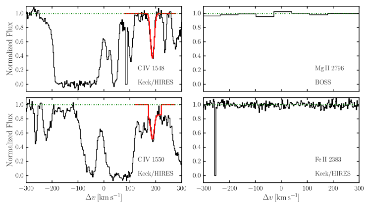
Figure 19: Absorption line spectrum of gas at $\sim 275$ kpc from the HzRG. The spectrum of the absorbing gas detected in the sightline of the quasar SDSS J1020$+$1040 at an impact parameter of $\sim 275$ kpc from the HzRG is shown. We found absorption from the high-ionization line C iv, offset by $188$ km s^-1 from the HzRG’s systemic redshift ($z=1.536$). No low-ionization-state metal absorption is detected; we show two representative non-detection, i.e. the first line of the Mg ii doublet, and Fe ii. The absorbing gas thus seems highly ionized. We fitted the C iv  absorption (red) and estimated a column density ${\rm log}[N_{\rm C\,IV}/{\rm cm}^{2}]=13.32\pm 0.02$. This absorber could be associated with the HzRG itself or with a companion object.

Appendix C Testing our Analysis Tools: PSF Subtraction and Lyman-Alpha Analysis

As described in section 3.2.1, we have presented results based on the CubExtractor package (Cantalupo in prep., Borisova et al. 2016), and showed the overall surface brightness, velocity, and dispersion maps as sum (along wavelength), first moment, and second moment of the flux distribution within the extracted three-dimensional mask (Fig. 6), respectively. Here we test our results by using a different method for the PSF subtraction and the analysis of the extended nebula. Specifically, we first compare the previously obtained maps with the maps obtained by using QDeblend^3D (Husemann et al. 2013) for the PSF subtraction. Secondly, we compare the moments analysis to a Gaussian fitting approach. Finding complete agreement between different techniques, both tests clearly show that our results are not affected by our method.

C.1 PSF Subtraction with QDeblend^3D

To study extended emission around AGN without contamination from the central source, Husemann et al. (2013) have developed the software tool QDeblend^3D, which differs from the method described in Borisova et al. (2016) and used in our analysis. We have thus used this tool to test our PSF subtraction. For completeness, we briefly summarise the iterative subtraction algorithm used in QDeblend^3D, but for further details we refer the reader to Husemann et al. (2013); Husemann et al. (2014) or to the manual of the software.

Whereas CubExtractor treats the IFU datacube as a sequence of layers for the PSF subtraction (section 3.2.1), QDeblend^3D considers each spaxel (spatial pixel of the cube) as an independent spectrum. In this framework, the spectrum of a point source differs in different spaxels only by a scale factor $s(x,y)$ defined by the PSF during observations. The relative strength of broad emission lines and the adjacent continuum can be used to constrain this scale factor for a quasar. More specifically, in the case of SDSS J1020$+$1040, QDeblend^3D extracts a high S/N quasar spectrum, from which we select the red portion of the Ly$\alpha$ line (to avoid the contamination from the Ly$\alpha$ forest) and the whole C iv  line emission as broad emission lines, and the interval $5300-5500$ Å as continuum. For each spaxel, these wavelength ranges are then used to determine $s(x,y)$ with respect to the high S/N quasar spectrum used as quasar template in the first iteration, i.e. $f_{\rm QSO,temp}(\lambda)$. QDeblend^3D then subtracts $s(x,y)f_{\rm QSO,temp}(\lambda)$ from the initial datacube. To avoid over-subtraction due to eventual host galaxy light on small scales, QDeblend^3D estimates this contribution $f_{\rm host}(\lambda)$ in a user-defined annulus from the residual datacube, subtracts it from $f_{\rm QSO,temp}(\lambda)$, and iteratively converges to a stable solution. This iterative procedure usually results in a PSF-subtracted datacube in 3-4 iterations. However, here we turn off the estimation of the host contribution to have a fair comparison with CubExtractor, which assumes the host to be much fainter than the quasar, and thus negligible. Indeed this should be the case for the bright quasar SDSS J1020$+$1040.

Having obtained the new PSF subtracted datacube using QDeblend^3D, we then extracted a new three dimensional mask for the ELAN, and computed the “optimally extracted” NB image, and the first and the second moments of the flux distribution as previously done with CubExtractor. Fig. 20 shows the comparison between the maps shown in Fig. 6 (i.e. PSF subtraction done with the CubExtractor package) and the new ones. For the purposes of this work (i.e. study of the structure on large scales), the maps are in complete agreement. However, we note that the residuals on very small scales ($\sim 1\arcsec$) greatly depends on the PSF normalization used and thus differs between the two methods. Notwithstanding these differences, the peak of the ELAN remains at the same position in close proximity to the location of SDSS J1020$+$1040, confirming the robustness of the detection of such emission at close separation.

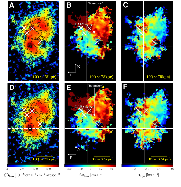
Figure 20: Testing the PSF subtraction: CubExtractor versus QDeblend^3D. (A), (B), and (C) as in Fig. 6. (D), (E), and (F) as in Fig. 6 but using QDeblend^3D (Husemann et al. 2013) for the PSF subtraction, instead of the CubExtractor package (Borisova et al. 2016). It is evident that our results do not depend on the PSF-subtraction algorithm used.

C.2 Analysis of the Ly$\alpha$ Nebula with KUBEVIZ: Gaussian Fit

In this section we show that a Gaussian can model in first approximation the kinematics of the Ly$\alpha$ emission within the whole nebula, resulting in complete agreement with the previous non-parametric approach, yielding consistent surface brightness, velocity shift and dispersion maps. To perform this additional analysis, we have used the custom IDL software KUBEVIZ (Fossati et al. 2016) to fit the Ly$\alpha$ emission within the ELAN. This code uses “linesets”, defined as groups of lines that are fitted simultaneously (e.g., H$\alpha$ and N ii). However, here, in the case of the Ly$\alpha$ line, the “lineset” is just a 1D Gaussian. Two symmetric windows free of contamination around each “lineset” are used to evaluate the continuum level. Before the fit, the datacube is smoothed in the spatial direction with a kernel of $3\times 3$ pixels (or $0.6\arcsec\times 0.6\arcsec$) to increase the S/N per pixel without compromising the spatial resolution of the data. No spectral smoothing is performed. During the fit, KUBEVIZ takes into account the noise from the variance datacube. However, the adopted variance underestimates the real error, most notably because it does not account for correlated noise introduced by resampling and smoothing (both applied while using KUBEVIZ). We therefore renormalize the final errors on the line fluxes assuming a $\chi^{2}=1$ per degree of freedom. In the end, we mask spaxels where the S/N in the Ly$\alpha$ line is $<2$ (see also Fossati et al. 2016 for more details). The results are shown in Fig. 21, and are in striking agreement with the “moments” analysis (section 3.2.1). Specifically, all the maps are consistent, showing (i) the same high surface brightness level (SB${}_{\rm Ly\alpha}\sim 10^{-17}{\rm\,erg\,s^{-1}\,cm^{-2}\,arcsec^{-2}}$), (ii) the same rotation-like pattern, and (iii) the same low velocity dispersion on large scales ($\sigma_{v}\approx 200$ km s^-1), while higher near compact objects.

To further stress the good agreement between the moments analysis and the Gaussian fit, we have computed the velocity shift within “Pseudo-slit 1” using a Gaussian fit, and compare it to the velocity curves shown in Fig. 10. Fig. 22 shows this test, reflecting once again the consistency between the two approaches for the system here studied. The similarity between the two different methods probably reveals that scattering of Ly$\alpha$ photons does not play an important role on the large scales of interest here ($\sim 100$ kpc), down to the current resolution.

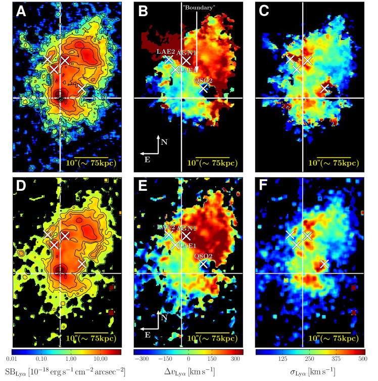
Figure 21: Testing the kinematic analysis of the ELAN: moments of the flux distribution versus Gaussian fit. (A), (B), and (C) as in Fig. 6. (D), (E), and (F) Ly$\alpha$ surface brightness, velocity shift from the systemic redshift of SDSS J1020$+$1040, and velocity dispersion within the ELAN obtained from a Gaussian fit with KUBEVIZ (Fossati et al. 2016). In both methods, the maps are smoothed with a $3$ pixels ($0.6\arcsec$) boxcar kernel. The similarity of the analysis with the two different methods (top and bottom row) is striking, probably revealing that scattering of Ly$\alpha$ photons does not play an important role on the large scales spanned by the ELAN, and down to the current spectral resolution.

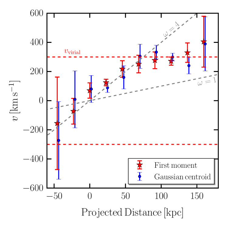
Figure 22: Ly$\alpha$ velocity centroids along “Pseudo-slit 1” through the ELAN: comparison between the first moment and a Gaussian fit. Velocity shift computed along pseudo-slit 1 using the first moment of the flux distribution (red, as in Fig. 10) or a Gaussian fit (blue). The data-points are estimated with respect to the position and systemic redshift of the quasar SDSS J1020$+$1040. In both cases, the errorbars show the 1$\sigma$ uncertainties. The red dashed line indicates the virial velocity $v_{\rm vir}=293$ km s^-1 for a halo of $M_{\rm DM}=10^{12.5}$ M_⊙. While the grey dashed lines represent the velocity curve for solid-body rotation with $\omega=1$, or $4$ in units of $3.1\times 10^{13}$ Hz. Once again we find good agreement between the moment analysis and the Gaussian fit.

Appendix D Our Cosmological Zoom-in Simulation

A powerful tool to interpret our observations comes from cosmological simulations of structure formation. The huge dynamical range involved in these types of simulations is the main limiting factor on the level of detail in modelling the gas physics.

Indeed, a complete simulation that can cover the full Ly$\alpha$ radiative transfer dynamics requires parsec resolution with a proper treatment of the mediums clumpiness (Verhamme et al. 2012). These high resolutions are only beginning to be achieved in cosmological simulations, and even so only in the inner regions of dark matter haloes where the galaxies reside and not in the CGM. On top of that coupling radiative transfer with gas hydrodynamics at these scales is still prohibitive in terms of CPU time.

To avoid the introduction of complex uncertainties and biases in our analysis, we thus decided to directly compare the observed velocity shear traced by the Ly$\alpha$ emission with the velocity patterns of the cool gas in a cosmological zoom-in simulation. Indeed, notwithstanding the challenges in play on small scales (e.g., McCourt et al. 2016), current cosmological simulations are able to follow in detail the overall distribution of the cool gas and its kinematics on the cosmological scales of ELANe (Goerdt & Ceverino 2015; Nelson et al. 2016; Dekel et al. 2009; Stewart et al. 2016).

D.1 The Simulated Halo

We have selected a system with the dark-matter halo mass at $z\approx 3$ similar to the expected value for DM haloes hosting quasars inferred from clustering studies at $z=2-3$, i.e. $M_{\rm DM}=10^{12.5}\,M_{\odot}$ (White et al. 2012; Fanidakis et al. 2013) ($M_{\rm DM}=10^{12.3\pm 0.5}$ for bright quasars; Trainor & Steidel 2012). Such a halo has been modelled within the test-runs of the high-resolution, “zoom-in” cosmological simulation suite NIHAO (Wang et al. 2015), and was not included in the original sample, which is limited to less massive systems (i.e. $M_{\rm star}<2\times 10^{11}$ M_⊙ at $z=0$). It is important to keep in mind that this selected halo has not been run with the aim of modelling our observations. Specifically, the massive halo has been simulated with the new version of the $N$-body SPH code, GASOLINE (Wadsley et al. 2004), which incorporates fundamental improvements for the hydro-solver as explained in Keller et al. (2014); Keller et al. (2015). The resulting halo has $M_{200}^{\rm DM}=10^{12.29}\,M_{\odot}$, $R_{200}=101$ kpc, and $M_{\rm star}=10^{10.77}\,M_{\odot}$ at $z=3$ (the snapshot closest to our observations). The system has been selected from a cosmological box of $90$ Mpc $h^{-1}$, which has been run with force softenings $\epsilon_{\rm DM}=0.7$ kpc $h^{-1}$, $\epsilon_{\rm gas}=0.3$ kpc $h^{-1}$, and particle masses $M_{\rm DM}=1.4\times 10^{7}\,M_{\odot}$, ${M_{\rm gas}=5\times 10^{6}\,M_{\odot}}$ for the highest refinement level for dark matter and gas, respectively. The simulation is based on the latest Planck cosmology (Planck Collaboration et al. 2014).

The code allows for metal diffusion as reported in Wadsley et al. (2008). The heating function takes into account photoionization and photoheating by a redshift-dependent UV background (Haardt & Madau 2012), while the cooling function includes the effects of metal lines and Compton scattering (Shen et al. 2010). Metal line cooling allows the gas to cool more efficiently and to temperatures below $10^{4}$ K. Specifically, the gas could reach temperatures as low as $\sim 100$ K in the densest regions with $n_{\rm H}\sim 10^{3.5}$ cm^-3 (Shen et al. 2010). A Kennicutt-Schmidt relation regulates star formation, with gas cooler than $15000$ K and denser than $10.3$ cm^-3 able to form stars. Stellar feedback includes two mechanisms: photoionizing radiation from pre-supernova massive stars (Stinson et al. 2013), and blast-waves from supernovae (Stinson et al. 2006). The version of the GASOLINE code used here does not include AGN feedback, which is often invoked to prevent the formation of galaxies with too high a stellar mass content in massive haloes (e.g., Schaye et al. 2015). However, at the redshift considered this feedback process should have marginal effects on the properties of the host galaxy of a quasar as the peak of the halo mass-stellar mass relation is moved at higher halo masses at $z=3$ with respect to $z=2$ (Moster et al. 2013). Indeed, the simulated halo agrees well with halo abundance matching measurements at $z=3$ (Moster et al. 2013; Behroozi et al. 2013), but starts to considerably overpredict the stellar mass for redshifts $z<1.5$.

D.1.1 A View of the Simulated Halo with Velocity Shear similar to Observations

To analyse the simulated halo and to select the orientation used in section 4.1, we proceed as follows. We focus on the snapshot at $z=3$, selecting a box of $4\times$ the virial radius of the halo, $L_{\rm box}=404$ kpc, centred on the massive halo. This box size has been chosen to encompass the whole size of the observed ELAN (if the centre of the halo is assumed to be SDSS J1020$+$1040). Next, we select the cool gas ($T<10^{4.5}$ K) within the selected region as this phase should be responsible for the Ly$\alpha$ emission (e.g., Gould & Weinberg 1996). Indeed, as stated in the main text and in section 4.3, the most favoured powering mechanism for the observed Ly$\alpha$ emission is photoionization from embedded sources in an optically thin regime. In this framework, the Ly$\alpha$ emission depends on the amount of cool gas and on its density, SB${}_{\rm Ly\alpha}\propto n_{\rm H}N_{\rm H}$ (e.g., Hennawi & Prochaska 2013). As current simulations seem to be unable to reproduce the high densities ($n_{\rm H}\gtrsim 1$ cm^-3) required by the ELANe on CGM scales (Arrigoni Battaia et al. 2015b; Hennawi et al. 2015), the most reliable tracer of the Ly$\alpha$ emission in simulations is the amount of cool gas, which simulations tend to correctly reproduce (Cantalupo et al. 2014). For this reason, we compute mass-weighted line-of-sight velocities and velocity dispersions for the cool gas to recover patterns visible in the observed Ly$\alpha$ maps (Fig. 6).

To find a view similar to our observations, we align our line-of-sight to the direction perpendicular to the angular momentum of the cool gas within the selected box. This simple requirement allow us to find the rotation-like pattern similar to the observations presented in Fig. 12. However, it is important to stress that many other directions would show a similar rotation pattern ($\sim 20$%; see section 4.1). To match the seeing of our dataset, we apply a Gaussian smoothing to the mass-weighted line-of-sight velocities and velocity dispersion maps before comparison (Fig. 12). The pseudo-slit orientation has been chosen to best cover the positive and negative shift of the line-of-sight velocity within the simulated halo, $140$ deg, which by chance happens to be close to the angle used for the slit in the observations, $149$ deg (E from N).

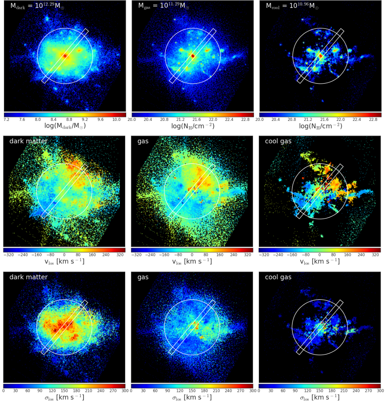
Figure 23: The simulated halo at $z=3$. We show the mass distribution (first row), mass-weighted line-of-sight velocities (second row), and velocity dispersion (third row) for dark matter (first column), gas (second column), and cool gas ($T<10^{4.5}$ K, third column) in a box of $\approx 400$ kpc centred on the simulated dark-matter halo and oriented as explained in the main text and in section D.1.1. The white circle gives the halo virial radius, $R_{200}=101$ kpc, while the white box represents the chord used for the comparison with the observations in Fig. 12. Note that the black corners are due to our analysis technique, i.e. we first select the volume and then analyse it.

In Fig. 23 we present the mass distribution (first row), mass-weighted line-of-sight velocity (second row), and mass-weighted velocity dispersion (third row) for the view of the simulated halo perpendicular to the angular momentum of the cool gas and discussed in section 4.1. In order to better highlight the presence of substructures, we show the raw (un-smoothed) images. Specifically, the first, second, and third column of Fig. 23 show the dark matter, gas, and cool gas, respectively. For each component (dark matter, gas, cool gas), the mass used for the weighting is the mass of the component itself at each particular location. The line-of-sight velocity maps once again reveal the rotation-like pattern discussed in the main text, while the velocity dispersion maps show very low values ($\sigma_{v}\sim 90$ km s^-1). The predicted velocity dispersions are thus smaller than the observed Ly$\alpha$ kinematics ($\sigma_{v}<270$ km s^-1). However we expect our simulation to show lower velocity dispersions than observations because of the combined effect of (i) the spectral resolution of MUSE at these wavelengths ($\sigma=72$ km s^-1), (ii) uncertainties on the mass for the quasar halo (i.e. the quasar SDSS J1020$+$1040 could reside in a more massive halo than here considered), and (iii) scattering of Ly$\alpha$ photons on small scales ($\lesssim 10$ kpc). Note that the (upper left and bottom right) black corners in all the simulated images are due to our strategy for the analysis, i.e. we first select the box and then rotate.

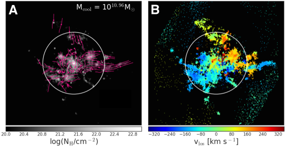
Figure 24: The rotation-like signal is due to inspiraling accreting cool gas. (A) cool gas ($T<10^{4.5}$ K) mass distribution (as total hydrogen column density) viewed through the same direction as in Fig. 12 and Fig. 23. The magenta lines indicate the velocity vector field in the plane of the image. It is clear the presence of an overall accreting pattern. (B) cool gas mass-weighted line-of-sight velocity. The rotation-like pattern is driven by inspiraling motions, whose accretion component is best visible in the in-plane velocity vector field in the left panel. The white circles indicate the halo virial radius, $R_{200}=101$ kpc.

Finally, by analysing the velocity vector field within the simulated halo, we confirm that the rotation-like pattern observed in our simulation is indeed due to inspiraling cool gaseous structures as expected by current theories (Fall & Efstathiou 1980; Stewart et al. 2016). In Fig. 24 we present this analysis. In particular, we overlay on the cool gas mass distribution the velocity vector field perpendicular to the line-of-sight (panel A). The substructures are clearly accreting towards the centre of the halo. This motion together with the line-of-sight motion (panel B), describes the inspiraling kinematics which we have argued to lead to the velocity shear visible in our observations.

Appendix E Photoionization: the Unlikely Case of a Large-scale Structure along the Line-of-sight

As a larger distance between the quasar SDSS J1020$+$1040 and the bright NW emission (i.e. $\gg 120$ kpc) could in principle explain the absence of He ii emission (because it would simply reduce the incidence of ionizing photons), and thus alleviate the tension in a photoionization scenario powered by the bright quasar (see section 4.3.2), we report here a calculation which assumes the ELAN is within the Hubble flow and along our line-of-sight. However, as anticipated in section 4.2, the photoionization modelling of such a projected structure requires a tuning of the physical properties of the emitting gas across at least $600$ kpc to reproduce the observed roughly constant SB_Lyα for the whole extent of the ELAN (Fig. 6). We explain this modelling in what follows.

Once again, we perform our calculations with the photoionization code Cloudy (Ferland et al. 2013) following the same assumptions as in section 4.3.2. However, we now assume a distance of $600$ kpc (or $300$ km s^-1 in the Hubble flow) for the NW emission. In Fig. 25 and Fig. 26 we show the prediction for this set of new models for $Z=0.1$, and $0.01$ Z_⊙ and compare them to the same constraints used in section 4.3.2. These models can reproduce the observed SB_Lyα together with the upper limits in the He ii and C iv lines (see panel A and compare with panels B and C in both Fig. 25 and Fig. 26). Specifically, the emitting gas in the NW part of the ELAN is now predicted to be optically thick (log$[N_{\rm HI}/{\rm cm}^{-2}]\gg 17.2$, see panels B) and to have $n_{\rm H}\gtrsim 10$ cm^-3 and $20\leq{\rm log}[N_{\rm H}/{\rm cm}^{-2}]\leq 22$, or $n_{\rm H}\gtrsim 0.3$ cm^-3 and $19\leq{\rm log}[N_{\rm H}/{\rm cm}^{-2}]\leq 22$, respectively for $Z=0.1$, and $0.01$ Z_⊙.

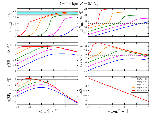
Figure 25: Photoionization modelling of the maximum within the NW redshifted emission assumed to be at $600$ kpc, $Z=0.1$ Z_⊙. The calculation has been performed using the photoionization code Cloudy (Ferland et al. 2013). We show, as a function of $n_{\rm H}$, the predicted SB_Lyα in units of $10^{-18}{\rm\,erg\,s^{-1}\,cm^{-2}\,arcsec^{-2}}$, the predicted column density of neutral hydrogen $N_{\rm HI}$, the predicted SB${}_{\rm He\,II}$ in units of $10^{-18}{\rm\,erg\,s^{-1}\,cm^{-2}\,arcsec^{-2}}$, the predicted column density of singly ionized helium $N_{\rm He\,II}$, the predicted SB${}_{\rm C\,IV}$ in units of $10^{-18}{\rm\,erg\,s^{-1}\,cm^{-2}\,arcsec^{-2}}$, and the ionization parameter $U$, respectively in (A), (B), (C), (D), (E), and (F). The solid horizontal lines show our measurement for SB_Lyα (together with shaded regions for the 1 and 2$\sigma$ uncertainties) and the upper limits for SB${}_{\rm He\,II}$ and SB${}_{\rm C\,IV}$. The horizontal dashed lines indicate the theoretical threshold dividing the optically thin regime from the optically thick case for that element. For neutral hydrogen is at $N_{\rm HI}=10^{17.2}$ cm^-2, while for helium is at $N_{\rm He\,II}=10^{17.8}$ cm^-2. If the quasar SDSS J1020$+$1040 is illuminating the emitting gas within a large-scale structure along the line-of-sight, optically thick models with $Z=0.1$ Z_⊙, $n_{\rm H}\gtrsim 10$ cm^-3 and $20\leq{\rm log}[N_{\rm H}/{\rm cm}^{-2}]\leq 22$ would match our observational constraints for the maximum within the NW redshifted emission.

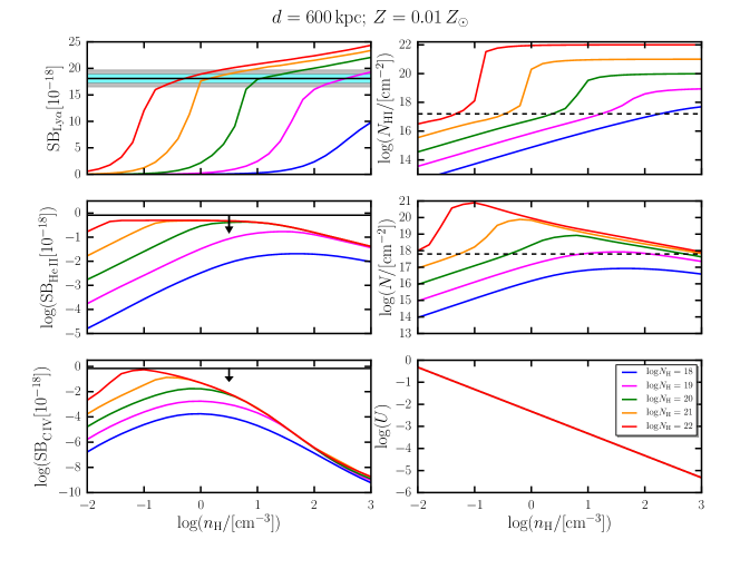
Figure 26: Photoionization modelling of the maximum within the NW redshifted emission assumed to be at $600$ kpc, $Z=0.01$ Z_⊙. The calculation has been performed using the photoionization code Cloudy (Ferland et al. 2013). We show, as a function of $n_{\rm H}$, the predicted SB_Lyα in units of $10^{-18}{\rm\,erg\,s^{-1}\,cm^{-2}\,arcsec^{-2}}$, the predicted column density of neutral hydrogen $N_{\rm HI}$, the predicted SB${}_{\rm He\,II}$ in units of $10^{-18}{\rm\,erg\,s^{-1}\,cm^{-2}\,arcsec^{-2}}$, the predicted column density of singly ionized helium $N_{\rm He\,II}$, the predicted SB${}_{\rm C\,IV}$ in units of $10^{-18}{\rm\,erg\,s^{-1}\,cm^{-2}\,arcsec^{-2}}$, and the ionization parameter $U$, respectively in (A), (B), (C), (D), (E), and (F). The solid horizontal lines show our measurement for SB_Lyα (together with shaded regions for the 1 and 2$\sigma$ uncertainties) and the upper limits for SB${}_{\rm He\,II}$ and SB${}_{\rm C\,IV}$. The horizontal dashed lines indicate the theoretical threshold dividing the optically thin regime from the optically thick case for that element. For neutral hydrogen is at $N_{\rm HI}=10^{17.2}$ cm^-2, while for helium is at $N_{\rm He\,II}=10^{17.8}$ cm^-2. If the quasar SDSS J1020$+$1040 is illuminating the emitting gas within a large-scale structure along the line-of-sight, optically thick models with $Z=0.01$ Z_⊙, $n_{\rm H}\gtrsim 0.3$ cm^-3 and $19\leq{\rm log}[N_{\rm H}/{\rm cm}^{-2}]\leq 22$ would match our observational constraints for the maximum within the NW redshifted emission.

Even though these models are closer to the expectation for the $n_{\rm H}$ and $N_{\rm H}$ in the CGM and IGM, they suffer of at least two considerable issues. First, the models that reproduce the observed Ly$\alpha$ emission are completely neutral (see panels B in Fig. 25 and Fig. 26). With such a high column of neutral hydrogen (log$[N_{\rm HI}/{\rm cm}^{-2}]\gtrsim 19$, see panels B), Ly$\alpha$ photons are expected to be heavily affected by resonant scattering effects. In particular, the bright NW emission should have a clear double peaked Ly$\alpha$ line profile (see e.g. Fig. 3 and 7 in Cantalupo et al. 2005). On the contrary, as discussed in section 4.2 and appendix C.2, the observed Ly$\alpha$ emission at the location of the NW bright clump, and more in general in the whole extent of the ELAN, can be approximated by a single Gaussian at our spectral resolution (FWHM $\approx 170$ km s^-1 at $5000$ Å).

Secondly, if the velocity shifts (e.g. Fig. 10) trace distances, i.e. a structure along the line-of-sight, there should be optically thin locations within the ELAN at smaller distances from the quasar SDSS J1020$+$1040 than the NW clump ($600$ kpc). In particular, given the known luminosity of the quasar SDSS J1020$+$1040, all the illuminated gas at $\lesssim 350$ kpc (or $\approx 175$ km s^-1 within the Hubble flow) will be optically thin. Basically, most of the ELAN between the quasar and the NW clump has to be optically thin while showing roughly the same level of SB_Lyα and similar non-detection in He ii and C iv as the optically thick gas at larger distances. In Fig. 27 we show the calculation performed with the Cloudy photoionization code (Ferland et al. 2013) for a distance of $300$ kpc (or $\approx 144$ km s^-1, or $\Delta z\approx 0.002$). The location of this region at $\approx 144$ km s^-1 from the quasar systemic is highlighted in Fig. 8 by the red dashed contour. This region has a slightly lower level of average emission (green shaded region in panel A of Fig. 27) than the NW clump (cyan shaded region in panel A of Fig. 27), i.e. SB${}_{\rm Ly\alpha}=(0.84\pm 0.05)\times 10^{-17}{\rm\,erg\,s^{-1}\,cm^{-2}\,arcsec^{-2}}$, but the same upper limits on He ii and C iv (as calculated in section 3.2.2). It is once again clear that only models with very high $n_{\rm H}\gtrsim 100$ cm^-3 and low $N_{\rm H}<10^{19}$ cm^-2 can reproduce simultaneously the observed SB_Lyα, and the upper limits in He ii and C iv (see panel A and compare with panels B and C in Fig. 27). As already discussed in section 4.3.2, such values are in contrast with current expectations for CGM and IGM gas, making it implausible that the quasar SDSS J1020$+$1040 illuminates the ELAN.

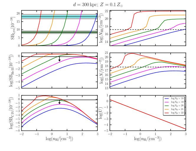
Figure 27: Photoionization modelling of the maximum within the NW redshifted emission assumed to be at $300$ kpc, $Z=0.1$ Z_⊙. The calculation has been performed using the photoionization code Cloudy (Ferland et al. 2013). We show, as a function of $n_{\rm H}$, the predicted SB_Lyα in units of $10^{-18}{\rm\,erg\,s^{-1}\,cm^{-2}\,arcsec^{-2}}$, the predicted column density of neutral hydrogen $N_{\rm HI}$, the predicted SB${}_{\rm He\,II}$ in units of $10^{-18}{\rm\,erg\,s^{-1}\,cm^{-2}\,arcsec^{-2}}$, the predicted column density of singly ionized helium $N_{\rm He\,II}$, the predicted SB${}_{\rm C\,IV}$ in units of $10^{-18}{\rm\,erg\,s^{-1}\,cm^{-2}\,arcsec^{-2}}$, and the ionization parameter $U$, respectively in (A), (B), (C), (D), (E), and (F). The solid horizontal lines show our measurement for SB_Lyα, together with shaded regions for the 1 and 2$\sigma$ uncertainties (in cyan for the NW clump at $\approx 120$ projected kpc; in green for the dashed region in panel E of Fig. 8). We also show the upper limits for SB${}_{\rm He\,II}$ and SB${}_{\rm C\,IV}$. The horizontal dashed lines indicate the theoretical threshold dividing the optically thin regime from the optically thick case for that element. For neutral hydrogen is at $N_{\rm HI}=10^{17.2}$ cm^-2, while for helium is at $N_{\rm He\,II}=10^{17.8}$ cm^-2. If the quasar SDSS J1020$+$1040 is illuminating the emitting gas within a large-scale structure along the line-of-sight, optically thick models with $Z=0.1$ Z_⊙, $n_{\rm H}\gtrsim 100$ cm^-3 and ${\rm log}[N_{\rm H}/{\rm cm}^{-2}]<19$ would match our observational constraints at $300$ kpc (or $\approx 144$ km s^-1) within the Hubble flow.

To solve these discrepancies, a scenario in which the gas is along the line-of-sight would require the quasar to be heavily obscured in the direction of the emitting gas, so that the ELAN does not receive its hard ionizing photons. Given that brighter AGN are expected to be able to disrupt the obscuring medium on small scales, and to have wider opening angles (Lawrence 1991; Kreimeyer & Veilleux 2013), the bright quasar SDSS J1020$+$1040 should radiate along the line-of-sight as it does towards us. This calculation therefore adds to the arguments against the ELAN being along the line-of-sight (presented in section 4.2). However, only planned follow-up observations at high spectral resolution, and additional observations to verify the powering mechanisms within this ELAN could verify our conclusion.

References

- Adelman-McCarthy & et al. (2009) Adelman-McCarthy J. K., et al. 2009, VizieR Online Data Catalog, 2294
- Allen et al. (2008) Allen M. G., Groves B. A., Dopita M. A., Sutherland R. S., Kewley L. J., 2008, ApJS, 178, 20
- Antonucci (1993) Antonucci R., 1993, ARA&A, 31, 473
- Aragón-Calvo et al. (2007) Aragón-Calvo M. A., van de Weygaert R., Jones B. J. T., van der Hulst J. M., 2007, ApJ, 655, L5
- Arrigoni Battaia et al. (2012) Arrigoni Battaia F., et al., 2012, A&A, 543, A112
- Arrigoni Battaia et al. (2015a) Arrigoni Battaia F., Yang Y., Hennawi J. F., Prochaska J. X., Matsuda Y., Yamada T., Hayashino T., 2015a, ApJ, 804, 26
- Arrigoni Battaia et al. (2015b) Arrigoni Battaia F., Hennawi J. F., Prochaska J. X., Cantalupo S., 2015b, ApJ, 809, 163
- Arrigoni Battaia et al. (2016) Arrigoni Battaia F., Hennawi J. F., Cantalupo S., Prochaska J. X., 2016, ApJ, 829, 3
- Bacon et al. (2010) Bacon R., et al., 2010, in Society of Photo-Optical Instrumentation Engineers (SPIE) Conference Series. , doi:10.1117/12.856027
- Becker et al. (1994) Becker R. H., White R. L., Helfand D. J., 1994, in Crabtree D. R., Hanisch R. J., Barnes J., eds, Astronomical Society of the Pacific Conference Series Vol. 61, Astronomical Data Analysis Software and Systems III. p. 165
- Behroozi et al. (2013) Behroozi P. S., Wechsler R. H., Conroy C., 2013, ApJ, 770, 57
- Bertin & Arnouts (1996) Bertin E., Arnouts S., 1996, Astronomy and Astrophysics Supplement, 117, 393
- Bolton et al. (2012) Bolton A. S., et al., 2012, AJ, 144, 144
- Borisova et al. (2016) Borisova E., et al., 2016, ApJ, 831, 39
- Bullock et al. (2001) Bullock J. S., Dekel A., Kolatt T. S., Kravtsov A. V., Klypin A. A., Porciani C., Primack J. R., 2001, ApJ, 555, 240
- Cabot et al. (2016) Cabot S. H. C., Cen R., Zheng Z., 2016, MNRAS, 462, 1076
- Cai et al. (2016) Cai Z., et al., 2016, preprint, (arXiv:1609.02913)
- Cai et al. (2017) Cai Z., et al., 2017, ApJ, 837, 71
- Caminha et al. (2016) Caminha G. B., et al., 2016, A&A, 595, A100
- Cantalupo et al. (2005) Cantalupo S., Porciani C., Lilly S. J., Miniati F., 2005, ApJ, 628, 61
- Cantalupo et al. (2014) Cantalupo S., Arrigoni-Battaia F., Prochaska J. X., Hennawi J. F., Madau P., 2014, Nature, 506, 63
- Cen & Zheng (2013) Cen R., Zheng Z., 2013, ApJ, 775, 112
- Christensen et al. (2006) Christensen L., Jahnke K., Wisotzki L., Sánchez S. F., 2006, A&A, 459, 717
- Codis et al. (2012) Codis S., Pichon C., Devriendt J., Slyz A., Pogosyan D., Dubois Y., Sousbie T., 2012, MNRAS, 427, 3320
- Condon & Broderick (1985) Condon J. J., Broderick J. J., 1985, AJ, 90, 2540
- Condon & Broderick (1986) Condon J. J., Broderick J. J., 1986, AJ, 91, 1051
- Condon et al. (1998) Condon J. J., Cotton W. D., Greisen E. W., Yin Q. F., Perley R. A., Taylor G. B., Broderick J. J., 1998, AJ, 115, 1693
- Crighton et al. (2015) Crighton N. H. M., Hennawi J. F., Simcoe R. A., Cooksey K. L., Murphy M. T., Fumagalli M., Prochaska J. X., Shanks T., 2015, MNRAS, 446, 18
- Curran et al. (2002) Curran S. J., Murphy M. T., Webb J. K., Rantakyrö F., Johansson L. E. B., Nikolić S., 2002, A&A, 394, 763
- Danovich et al. (2015) Danovich M., Dekel A., Hahn O., Ceverino D., Primack J., 2015, MNRAS, 449, 2087
- De Breuck et al. (2000) De Breuck C., Röttgering H., Miley G., van Breugel W., Best P., 2000, A&A, 362, 519
- Dekel & Birnboim (2006) Dekel A., Birnboim Y., 2006, MNRAS, 368, 2
- Dekel & Silk (1986) Dekel A., Silk J., 1986, ApJ, 303, 39
- Dekel et al. (2009) Dekel A., et al., 2009, Nature, 457, 451
- Dey et al. (2005) Dey A., et al., 2005, ApJ, 629, 654
- Dijkstra & Loeb (2008) Dijkstra M., Loeb A., 2008, MNRAS, 386, 492
- Dijkstra & Loeb (2009) Dijkstra M., Loeb A., 2009, MNRAS, 400, 1109
- Dijkstra et al. (2006) Dijkstra M., Haiman Z., Spaans M., 2006, ApJ, 649, 14
- Djorgovski et al. (2007) Djorgovski S. G., Courbin F., Meylan G., Sluse D., Thompson D., Mahabal A., Glikman E., 2007, ApJ, 662, L1
- Douglas et al. (1996) Douglas J. N., Bash F. N., Bozyan F. A., Torrence G. W., Wolfe C., 1996, AJ, 111, 1945
- Draine (2011) Draine B. T., 2011, Physics of the Interstellar and Intergalactic Medium
- Duval et al. (2014) Duval F., Schaerer D., Östlin G., Laursen P., 2014, A&A, 562, A52
- Ekers (1969) Ekers J. A., 1969, Australian Journal of Physics Astrophysical Supplement, 7
- Ellison et al. (2008) Ellison S. L., York B. A., Pettini M., Kanekar N., 2008, MNRAS, 388, 1349
- Emonts et al. (2016) Emonts B. H. C., et al., 2016, Science, 354, 1128
- Fall & Efstathiou (1980) Fall S. M., Efstathiou G., 1980, MNRAS, 193, 189
- Fanidakis et al. (2013) Fanidakis N., Macciò A. V., Baugh C. M., Lacey C. G., Frenk C. S., 2013, MNRAS, 436, 315
- Fardal et al. (2001) Fardal M. A., Katz N., Gardner J. P., Hernquist L., Weinberg D. H., Davé R., 2001, ApJ, 562, 605
- Farina et al. (2013) Farina E. P., Montuori C., Decarli R., Fumagalli M., 2013, MNRAS, 431, 1019
- Faucher-Giguère & Kereš (2011) Faucher-Giguère C.-A., Kereš D., 2011, MNRAS, 412, L118
- Faucher-Giguère et al. (2010) Faucher-Giguère C.-A., Kereš D., Dijkstra M., Hernquist L., Zaldarriaga M., 2010, ApJ, 725, 633
- Ferland et al. (2013) Ferland G. J., et al., 2013, Rev. Mex. Astron. Astrofis., 49, 137
- Fossati et al. (2016) Fossati M., Fumagalli M., Boselli A., Gavazzi G., Sun M., Wilman D. J., 2016, MNRAS, 455, 2028
- Fumagalli et al. (2011) Fumagalli M., Prochaska J. X., Kasen D., Dekel A., Ceverino D., Primack J. R., 2011, MNRAS, 418, 1796
- Fumagalli et al. (2016) Fumagalli M., Cantalupo S., Dekel A., Morris S. L., O’Meara J. M., Prochaska J. X., Theuns T., 2016, preprint, (arXiv:1607.03893)
- Furlanetto et al. (2005) Furlanetto S. R., Schaye J., Springel V., Hernquist L., 2005, ApJ, 622, 7
- Geach et al. (2016) Geach J. E., et al., 2016, preprint, (arXiv:1608.02941)
- Geller et al. (2014) Geller M. J., Hwang H. S., Diaferio A., Kurtz M. J., Coe D., Rines K. J., 2014, ApJ, 783, 52
- Gibson et al. (2009) Gibson R. R., et al., 2009, ApJ, 692, 758
- Goerdt & Ceverino (2015) Goerdt T., Ceverino D., 2015, MNRAS, 450, 3359
- Gott (1975) Gott III J. R., 1975, ApJ, 201, 296
- Gould & Weinberg (1996) Gould A., Weinberg D. H., 1996, ApJ, 468, 462
- Haardt & Madau (2012) Haardt F., Madau P., 2012, ApJ, 746, 125
- Haiman et al. (2000) Haiman Z., Spaans M., Quataert E., 2000, ApJ, 537, L5
- Hainline et al. (2011) Hainline K. N., Shapley A. E., Greene J. E., Steidel C. C., 2011, ApJ, 733, 31
- Harrison et al. (2012) Harrison C. M., et al., 2012, MNRAS, 426, 1073
- Harrison et al. (2014) Harrison C. M., Alexander D. M., Mullaney J. R., Swinbank A. M., 2014, MNRAS, 441, 3306
- Heckman et al. (1991a) Heckman T. M., Miley G. K., Lehnert M. D., van Breugel W., 1991a, ApJ, 370, 78
- Heckman et al. (1991b) Heckman T. M., Lehnert M. D., Miley G. K., van Breugel W., 1991b, ApJ, 381, 373
- Hennawi & Prochaska (2013) Hennawi J. F., Prochaska J. X., 2013, ApJ, 766, 58 (QPQ4)
- Hennawi et al. (2006) Hennawi J. F., et al., 2006, AJ, 131, 1
- Hennawi et al. (2015) Hennawi J. F., Prochaska J. X., Cantalupo S., Arrigoni-Battaia F., 2015, Science, 348, 779
- Herenz et al. (2015) Herenz E. C., Wisotzki L., Roth M., Anders F., 2015, A&A, 576, A115
- Hewett & Wild (2010) Hewett P. C., Wild V., 2010, MNRAS, 405, 2302
- Hoyle (1951) Hoyle F., 1951, in Problems of Cosmical Aerodynamics. p. 195
- Hu & Cowie (1987) Hu E. M., Cowie L. L., 1987, ApJ, 317, L7
- Hubble (1929) Hubble E., 1929, Proceedings of the National Academy of Science, 15, 168
- Humphrey et al. (2008) Humphrey A., Villar-Martín M., Vernet J., Fosbury R., di Serego Alighieri S., Binette L., 2008, MNRAS, 383, 11
- Husemann et al. (2013) Husemann B., Wisotzki L., Sánchez S. F., Jahnke K., 2013, A&A, 549, A43
- Husemann et al. (2014) Husemann B., Jahnke K., Sánchez S. F., Wisotzki L., Nugroho D., Kupko D., Schramm M., 2014, MNRAS, 443, 755
- Kakkad et al. (2016) Kakkad D., et al., 2016, A&A, 592, A148
- Keller et al. (2014) Keller B. W., Wadsley J., Benincasa S. M., Couchman H. M. P., 2014, MNRAS, 442, 3013
- Keller et al. (2015) Keller B. W., Wadsley J., Couchman H. M. P., 2015, MNRAS, 453, 3499
- Kellermann et al. (1989) Kellermann K. I., Sramek R., Schmidt M., Shaffer D. B., Green R., 1989, AJ, 98, 1195
- Kent & Gunn (1982) Kent S. M., Gunn J. E., 1982, AJ, 87, 945
- Kereš et al. (2005) Kereš D., Katz N., Weinberg D. H., Davé R., 2005, MNRAS, 363, 2
- Kereš et al. (2009) Kereš D., Katz N., Fardal M., Davé R., Weinberg D. H., 2009, MNRAS, 395, 160
- Kollmeier et al. (2010) Kollmeier J. A., Zheng Z., Davé R., Gould A., Katz N., Miralda-Escudé J., Weinberg D. H., 2010, ApJ, 708, 1048
- Kreimeyer & Veilleux (2013) Kreimeyer K., Veilleux S., 2013, ApJ, 772, L11
- Lacy et al. (2013) Lacy M., et al., 2013, ApJS, 208, 24
- Lau et al. (2016) Lau M. W., Prochaska J. X., Hennawi J. F., 2016, ApJS, 226, 25
- Lawrence (1991) Lawrence A., 1991, MNRAS, 252, 586
- Lusso et al. (2015) Lusso E., Worseck G., Hennawi J. F., Prochaska J. X., Vignali C., Stern J., O’Meara J. M., 2015, MNRAS, 449, 4204
- Martin et al. (2014) Martin D. C., Chang D., Matuszewski M., Morrissey P., Rahman S., Moore A., Steidel C. C., 2014, ApJ, 786, 106
- Martin et al. (2015) Martin D. C., Matuszewski M., Morrissey P., Neill J. D., Moore A., Cantalupo S., Prochaska J. X., Chang D., 2015, Nature, 524, 192
- Matsuda et al. (2005) Matsuda Y., et al., 2005, ApJ, 634, L125
- Matsuda et al. (2009) Matsuda Y., et al., 2009, MNRAS, 400, L66
- McCarthy (1993) McCarthy P. J., 1993, ARA&A, 31, 639
- McCourt et al. (2016) McCourt M., Oh S. P., O’Leary R. M., Madigan A.-M., 2016, preprint, (arXiv:1610.01164)
- Miley et al. (2006) Miley G. K., et al., 2006, ApJ, 650, L29
- More et al. (2015) More S., Diemer B., Kravtsov A. V., 2015, ApJ, 810, 36
- Mori et al. (2004) Mori M., Umemura M., Ferrara A., 2004, ApJ, 613, L97
- Moster et al. (2013) Moster B. P., Naab T., White S. D. M., 2013, MNRAS, 428, 3121
- Nagao et al. (2006) Nagao T., Maiolino R., Marconi A., 2006, A&A, 459, 85
- Nelson et al. (2016) Nelson D., Genel S., Pillepich A., Vogelsberger M., Springel V., Hernquist L., 2016, MNRAS,
- Nesvadba et al. (2011) Nesvadba N. P. H., Polletta M., Lehnert M. D., Bergeron J., De Breuck C., Lagache G., Omont A., 2011, MNRAS, 415, 2359
- Neufeld (1990) Neufeld D. A., 1990, ApJ, 350, 216
- North et al. (2012) North P. L., Courbin F., Eigenbrod A., Chelouche D., 2012, A&A, 542, A91
- O’Meara et al. (2015) O’Meara J. M., et al., 2015, AJ, 150, 111
- Oke (1974) Oke J. B., 1974, ApJS, 27, 21
- Oser et al. (2010) Oser L., Ostriker J. P., Naab T., Johansson P. H., Burkert A., 2010, ApJ, 725, 2312
- Osterbrock (1989) Osterbrock D. E., 1989, Astrophysics of gaseous nebulae and active galactic nuclei
- Ouchi et al. (2010) Ouchi M., et al., 2010, ApJ, 723, 869
- Pâris et al. (2012) Pâris I., et al., 2012, A&A, 548, A66
- Peebles (1969) Peebles P. J. E., 1969, ApJ, 155, 393
- Persic et al. (1996) Persic M., Salucci P., Stel F., 1996, MNRAS, 281, 27
- Pilkington & Scott (1965) Pilkington J. D. H., Scott J. F., 1965, Mem. RAS, 69, 183
- Planck Collaboration et al. (2014) Planck Collaboration et al., 2014, A&A, 571, A16
- Pontzen et al. (2013) Pontzen A., Roškar R., Stinson G. S., Woods R., Reed D. M., Coles J., Quinn T. R., 2013, pynbody: Astrophysics Simulation Analysis for Python
- Porciani et al. (2002) Porciani C., Dekel A., Hoffman Y., 2002, MNRAS, 332, 339
- Prescott et al. (2008) Prescott M. K. M., Kashikawa N., Dey A., Matsuda Y., 2008, ApJ, 678, L77
- Prescott et al. (2009) Prescott M. K. M., Dey A., Jannuzi B. T., 2009, ApJ, 702, 554
- Prescott et al. (2011) Prescott M. K. M., Smith P. S., Schmidt G. D., Dey A., 2011, ApJ, 730, L25
- Prescott et al. (2013) Prescott M. K. M., Dey A., Jannuzi B. T., 2013, ApJ, 762, 38
- Prescott et al. (2015a) Prescott M. K. M., Martin C. L., Dey A., 2015a, ApJ, 799, 62
- Prescott et al. (2015b) Prescott M. K. M., Martin C. L., Dey A., 2015b, ApJ, 799, 62
- Prochaska & Hennawi (2009) Prochaska J. X., Hennawi J. F., 2009, ApJ, 690, 1558
- Prochaska et al. (2011) Prochaska J. X., Weiner B., Chen H.-W., Mulchaey J., Cooksey K., 2011, ApJ, 740, 91
- Prochaska et al. (2013a) Prochaska J. X., Hennawi J. F., Simcoe R. A., 2013a, ApJ, 762, L19 (QPQ5)
- Prochaska et al. (2013b) Prochaska J. X., et al., 2013b, ApJ, 776, 136
- Prochaska et al. (2014) Prochaska J. X., Lau M. W., Hennawi J. F., 2014, ApJ, 796, 140
- Richards et al. (2011) Richards G. T., et al., 2011, AJ, 141, 167
- Richardson et al. (2012) Richardson J., Zheng Z., Chatterjee S., Nagai D., Shen Y., 2012, ApJ, 755, 30
- Roche et al. (2014) Roche N., Humphrey A., Binette L., 2014, MNRAS, 443, 3795
- Rosdahl & Blaizot (2012) Rosdahl J., Blaizot J., 2012, MNRAS, 423, 344
- Rubin et al. (2014) Rubin K. H. R., Prochaska J. X., Koo D. C., Phillips A. C., Martin C. L., Winstrom L. O., 2014, ApJ, 794, 156
- Rudie et al. (2012) Rudie G. C., et al., 2012, ApJ, 750, 67
- Saito et al. (2006) Saito T., Shimasaku K., Okamura S., Ouchi M., Akiyama M., Yoshida M., 2006, ApJ, 648, 54
- Scannapieco et al. (2008) Scannapieco C., Tissera P. B., White S. D. M., Springel V., 2008, MNRAS, 389, 1137
- Schaye et al. (2015) Schaye J., et al., 2015, MNRAS, 446, 521
- Shapley et al. (2003) Shapley A. E., Steidel C. C., Pettini M., Adelberger K. L., 2003, ApJ, 588, 65
- Sharma & Steinmetz (2005) Sharma S., Steinmetz M., 2005, ApJ, 628, 21
- Shen et al. (2010) Shen S., Wadsley J., Stinson G., 2010, MNRAS, 407, 1581
- Shen et al. (2016) Shen Y., et al., 2016, ApJ, 831, 7
- Sijacki et al. (2007) Sijacki D., Springel V., Di Matteo T., Hernquist L., 2007, MNRAS, 380, 877
- Silk & Rees (1998) Silk J., Rees M. J., 1998, A&A, 331, L1
- Skrutskie et al. (2006) Skrutskie M. F., et al., 2006, AJ, 131, 1163
- Steidel et al. (2010) Steidel C. C., Erb D. K., Shapley A. E., Pettini M., Reddy N., Bogosavljević M., Rudie G. C., Rakic O., 2010, ApJ, 717, 289
- Stern et al. (2016) Stern J., Hennawi J. F., Prochaska J. X., Werk J. K., 2016, preprint, (arXiv:1604.02168)
- Stewart et al. (2011) Stewart K. R., Kaufmann T., Bullock J. S., Barton E. J., Maller A. H., Diemand J., Wadsley J., 2011, ApJ, 738, 39
- Stewart et al. (2016) Stewart K., et al., 2016, preprint, (arXiv:1606.08542)
- Stinson et al. (2006) Stinson G., Seth A., Katz N., Wadsley J., Governato F., Quinn T., 2006, MNRAS, 373, 1074
- Stinson et al. (2013) Stinson G. S., Brook C., Macciò A. V., Wadsley J., Quinn T. R., Couchman H. M. P., 2013, MNRAS, 428, 129
- Stockton et al. (2006) Stockton A., Fu H., Canalizo G., 2006, New Astron. Rev., 50, 694
- Stuik et al. (2006) Stuik R., Bacon R., Conzelmann R., Delabre B., Fedrigo E., Hubin N., Le Louarn M., Ströbele S., 2006, New Astron. Rev., 49, 618
- Swinbank et al. (2015) Swinbank A. M., et al., 2015, MNRAS, 449, 1298
- Taniguchi & Shioya (2000) Taniguchi Y., Shioya Y., 2000, ApJ, 532, L13
- Tonnesen & Bryan (2011) Tonnesen S., Bryan G. L., 2011, ApJ, 727, 133
- Trainor & Steidel (2012) Trainor R. F., Steidel C. C., 2012, ApJ, 752, 39
- Tumlinson et al. (2013) Tumlinson J., et al., 2013, ApJ, 777, 59
- Venemans et al. (2007) Venemans B. P., et al., 2007, A&A, 461, 823
- Verhamme et al. (2006) Verhamme A., Schaerer D., Maselli A., 2006, A&A, 460, 397
- Verhamme et al. (2012) Verhamme A., Dubois Y., Blaizot J., Garel T., Bacon R., Devriendt J., Guiderdoni B., Slyz A., 2012, A&A, 546, A111
- Véron-Cetty & Véron (2010) Véron-Cetty M.-P., Véron P., 2010, A&A, 518, A10
- Villar-Martín et al. (2003) Villar-Martín M., Vernet J., di Serego Alighieri S., Fosbury R., Humphrey A., Pentericci L., 2003, MNRAS, 346, 273
- Vogelsberger et al. (2014) Vogelsberger M., et al., 2014, MNRAS, 444, 1518
- Vogt et al. (1994) Vogt S. S., et al., 1994, in Proc. SPIE Instrumentation in Astronomy VIII, David L. Crawford; Eric R. Craine; Eds., Volume 2198, p. 362. pp 362–+
- Wadsley et al. (2004) Wadsley J. W., Stadel J., Quinn T., 2004, New Astron., 9, 137
- Wadsley et al. (2008) Wadsley J. W., Veeravalli G., Couchman H. M. P., 2008, MNRAS, 387, 427
- Wang et al. (2015) Wang L., Dutton A. A., Stinson G. S., Macciò A. V., Penzo C., Kang X., Keller B. W., Wadsley J., 2015, MNRAS, 454, 83
- Weilbacher et al. (2014) Weilbacher P. M., Streicher O., Urrutia T., Pécontal-Rousset A., Jarno A., Bacon R., 2014, in Manset N., Forshay P., eds, Astronomical Society of the Pacific Conference Series Vol. 485, Astronomical Data Analysis Software and Systems XXIII. p. 451 (arXiv:1507.00034)
- White & Becker (1992) White R. L., Becker R. H., 1992, ApJS, 79, 331
- White & Rees (1978) White S. D. M., Rees M. J., 1978, MNRAS, 183, 341
- White et al. (2012) White M., et al., 2012, MNRAS, 424, 933
- Yang et al. (2006) Yang Y., Zabludoff A. I., Davé R., Eisenstein D. J., Pinto P. A., Katz N., Weinberg D. H., Barton E. J., 2006, ApJ, 640, 539
- Yang et al. (2009) Yang Y., Zabludoff A., Tremonti C., Eisenstein D., Davé R., 2009, ApJ, 693, 1579
- Yang et al. (2014) Yang Y., Zabludoff A., Jahnke K., Davé R., 2014, ApJ, 793, 114
- Zhang et al. (2009) Zhang Y., Yang X., Faltenbacher A., Springel V., Lin W., Wang H., 2009, ApJ, 706, 747
- Zjupa & Springel (2017) Zjupa J., Springel V., 2017, MNRAS, 466, 1625
- van den Bosch et al. (2002) van den Bosch F. C., Abel T., Croft R. A. C., Hernquist L., White S. D. M., 2002, ApJ, 576, 21