Oscillator-based Ising Machine

Abstract

Many combinatorial optimization problems can be mapped to finding the ground states of the corresponding Ising Hamiltonians. The physical systems that can solve optimization problems in this way, namely Ising machines, have been attracting more and more attention recently. Our work shows that Ising machines can be realized using almost any nonlinear self-sustaining oscillators with logic values encoded in their phases. Many types of such oscillators are readily available for large-scale integration, with potentials in high-speed and low-power operation. In this paper, we describe the operation and mechanism of oscillator-based Ising machines. The feasibility of our scheme is demonstrated through several examples in simulation and hardware, among which a simulation study reports average solutions exceeding those from state-of-art Ising machines on a benchmark combinatorial optimization problem of size 2000.

I Introduction

The Ising model, named after physicist Ernest Ising, started as a model for explaining domain formation in ferromagnets [1] Nowadays, it is considered as a promising non-von Neumann architecture for solving many combinatorial optimization problems [2, 3]. In these problems, the objective to be minimized is usually formulated as the energy of a collection of spins $\{s_{i}\}$, $i=1,\cdots,n$, represented by a Hamiltonian function:

$$H=\sum_{i}h_{i}s_{i}+\sum_{i,j}J_{ij}s_{i}s_{j},$$ (1)

where $s_{i}\in\{-1,~{}+1\}$ are binary integers; coefficients $\{J_{ij}\}$ and $\{h_{i}\}$ are real numbers.

An equivalent formula of the Hamiltonian can be written as follows.

$$H=\sum_{i,j}J_{ij}s_{i}s_{j},$$ (2)

where $\{s_{i}\}$’s size is increased by one, with the last one $s_{n+1}\equiv+1$; $\{J_{ij}\}$’s dimension is also increased by one, with $J_{n+1,k}=J_{k,n+1}=h_{k}/2$ for $k=1,\cdots,n$.

An Ising machine is a physical realization of the Ising model, i.e., it is a physical system that can minimize the Hamiltonian function defined in 1 or 2. Such a system normally has a graph structure, where the vertices/nodes represent the spins $\{s_{i}\}$ and the edges encode the coupling coefficients $\{J_{ij}\}$ and $\{h_{i}\}$. The Ising Hamiltonian can normally be mapped to the energy of this physical system. Through annealing, once the system’s energy is minimized, the nodes encode the globally optimal spin configuration, aka, the ground state.

Several schemes have been proposed towards the realization of Ising machines. Perhaps the best-known example comes from D-Wave Systems [4, 5]. Their quantum annealers use superconducting loops as nodes and interconnect them with Josephson junctions [6]. Their computing environment requires a temperature below 80mK [4]. There is a lot of controversy [7] around their advantages over simulated annealing run on classical computers. It is believed that through a mechanism known as quantum tunnelling they offer the largest speed-up on problems with rugged energy landscapes [8].

Classical annealers that do not rely on quantum mechanics to function have also been reported with good performances. One type of annealers use time-multiplexed optical parametric oscillators (OPOs) as the Ising spins, couple them through delay lines, and control the coupling with an FPGA [9, 10]. An Ising machine with a size of 2000 has been reported with a high success probability for solving the MAX-CUT problems [11]. Similar to OPOs, mechanical parametric oscillators built with MEMS technology have also been proposed to use in Ising machines [12]; no physical realization has been reported yet. Nanomagnets with low energy barriers are another candidate for Ising spins [13]. They are given a name “p-bits”, and are shown through computational studies to be able to minimize energy functions, which stem from not only combinatorial optimization problems, but also invertible logic computation [14]. Researchers have also been exploring the possibility of implementing Ising machines with SRAMs in CMOS technology [15]. But “the efficacy in achieving a global energy minimum is limited” [15] due to variation. The speed-up and accuracy reported by [15] are instead based on deterministic on-chip computation paired with external random number generators — a digital hardware implementation of the simulated annealing algorithm. As such, the CMOS-based scheme is not directly comparable to the other Ising machines described above.

In this paper, we report a new finding: almost any nonlinear oscillator is suitable for implementing Ising machines. Nowadays, a broad choice of such oscillators are available from not just CMOS technology, but also optics, MEMS, spin torque devices, biochemical reaction networks, etc., among which many are integrable and highly energy-efficient. Therefore, such a finding greatly expands the scope of the physical realization of Ising machines.

The mechanism is based on a common phenomenon observed in almost all nonlinear oscillators — injection locking. A variant of it — sub-harmonic injection locking (SHIL) can excite multiple stable phase-locked responses in oscillators [16, 17, 18]. For example, when an oscillator is perturbed by an external periodic input at close to twice its natural frequency, the oscillator’s injection-locked response is bistable. The bistable states differ only in the phase/timing and it can be proven that their phase difference is $180^{\circ}$ [16, 17]. In this way, almost any oscillator can be used as a binary logic latch, with the logic value encoded in the phase of oscillation. Recently, it has been demonstrated that it is feasible to use oscillators and phase-based encoding to build finite state machines for general-purpose Boolean computation based on the conventional von Neumann architecture [19, 20, 17].

In this paper, we take the oscillator-based Boolean computation idea one step further. An oscillator under SHIL can store a binary logic value securely if the external periodic perturbation is strong. As we reduce the strength of this perturbation, SHIL becomes weaker. And because of the intrinsic phase noise, the oscillator will “degrade” from a binary latch to a binary random number generator. Naturally, we can speculate that when a few such random number generators are coupled together, their values will prefer certain configurations over others. By properly designing the coupling between them, we can encode the Ising Hamiltonian in a network of such coupled oscillators so that the ground state is the most preferable state with the lowest “energy”. In Sec. II, we expand on this idea and explore the relationship between the “energy” of coupled oscillators and the Ising Hamiltonian.

It is worth noting that computation with coupled oscillators is not a new topic. Associated memory arrays made with oscillators have been attracting research interest for many years [21, 22, 23]. They are shown to be suitable for some specialized non-Boolean computational tasks, such as image recognition, edge detection, etc. But an Ising machine differs from them in its capabilities in solving general combinatorial optimization problems and invertible logic problems [14], which are in the Boolean computation domain. The enabling technique is the use of SHIL to digitize an oscillator’s phase, which has recently been studied in the context of oscillator-based finite state machines. Adapting the technique in realizing Ising machines has become a feasible option and a natural choice. It is also an important piece in the framework of oscillator-based Boolean computation. Indeed, with oscillators, both Ising machines, which are stochatic in nature, and deterministic digital computation can be implemented with the same type of devices, possibly on the same chip, opening up many new possibilities in the design of computer architectures and algorithms.

It is also known that oscillations of neurons in cortical networks play an important role in many of the functionalities of neural circuits, ranging from sensory input processing to working memory retention and decision making. It has long been suspected that the coupled oscillating neurons function as an optimizer [24]. While associative memory arrays offer a perspective for understanding this hypophysis, oscillator-based Ising machines offer another one, showing that it is possible for coupled oscillators to solve for almost arbitrarily complicated problems. In fact, Ising machines can encode any Boolean logic function and are Turing complete [3]. The bistability or multistability, instead of coming from SHIL, can also come from delayed coupling [25].

In the remainder of this paper, we first describe the idea and mechanism of oscillator-based Ising machines in Sec. II. In particular, we show how the global Lyapunov function of the phase macromodel of coupled oscillators maps to the Ising Hamiltonian. We also study how variations in the oscillators’ central frequencies affect the performance of the system. Then in Sec. III, we study how the speed of convergence scales with the size of the optimization problem, which is often considered as a major attractiveness of Ising machines. Several examples of the use of oscillator-based Ising machines are shown in Sec. IV, including in both combinatorial optimization problems and invertible logic applications.

II Oscillator-based Ising Machines

In this section, we first sketch out the idea of using oscillators to implement Ising machines, focusing on the intuition behind it. Then we describe the mechanism more rigorously by deriving the phase macromodel of coupled oscillators and studying its relationship with the Ising Hamiltonian.

As mentioned in Sec. I, when an oscillator with natural frequency $f_{0}$ is perturbed by a small periodic external input at $f_{1}\approx f_{0}$, through injection locking, its response can lock on to the input in both frequency and phase. Many natural phenomena result from this mechanism, e.g., metronomes on a same platform end up ticking in unison (Figure 1), fireflies synchronize their flashes, neurons fire in unison, etc. Sub-harmonic injection locking (SHIL) is a special type of injection locking. Under SHIL, an oscillator is perturbed by a periodic input at about twice its natural frequency, i.e., $2f_{1}$; we call this perturbation a synchronization signal (SYNC). The oscillator will then lock to the sub-harmonic of SYNC while developing bistable phase locks separated by 180^∘. In this way, it becomes a logic latch that can store a phase-based binary bit. Together with phase-based combinational logic gates [19], finite state machines can then be implemented for general-purpose Boolean computation. This mechanism is generic in almost all oscillators; the scheme is not specific to electrical ones. A broad choice of nonlinear oscillators — from MEMS oscillators to optical lasers, from spin-torque nano-oscillators (STNOs) to oscillating biochemical reactions and neurons — become potential candidates for Boolean computation systems (Figure 1).

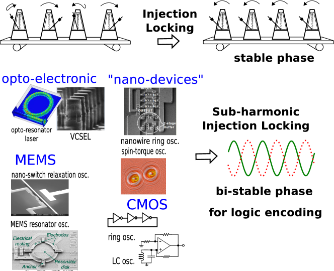
Figure 1: Injection Locking leads to phase lock. In the case of SHIL, bistable phase locks enable phase-based logic encoding and storage with many types of nano oscillators.

Furthermore, if we lower SYNC and reduce the effect of SHIL, due to intrinsic phase noise and detuning, the oscillator will have phase response that stochastically flips between the bistable states — it becomes a binary random number generator. If two of these oscillators are coupled, e.g., through resistive connection, instead of having four states {00}, {01}, {10}, {11} with even probabilities, they will have higher probability to end up in {00} and {11} — these two states become the ground states of this simple size-2 Ising model. More complicated Ising Hamiltonians can be encoded by coupling more oscillators, in a similar way to the existing Ising machine proposals. Specifically, a larger coefficient $J_{ij}$ in 2 is represented with a larger conductance in the resistive connection.

To study this mechanism more properly, we start from the phase macromodel of a single nonlinear self-sustaining oscillator. Such an oscillator under perturbation can be described mathematically as a set of Differential Algebraic Equations (DAEs):

$$\frac{d}{dt}\vec{q}(\vec{x})+\vec{f}(\vec{x})+\vec{b}(t)=\vec{0}$$ (3)

where $\vec{x}\in\mathbf{R}^{n}$ are the unknowns in the system, $\vec{b}(t)$ is a small time-varying input. The oscillator’s response can be approximated well as

$$\vec{x}(t)=\vec{x}_{s}(t+\alpha(t))$$ (4)

where $x_{s}(t)$ is the oscillator’s steady state response without perturbation ($\vec{b}(t)\equiv\vec{0}$); $\alpha(t)$ is the phase shift caused by the external input and is governed by the following differential equation:

$$\frac{d}{dt}\alpha(t)=\vec{v}^{T}(t+\alpha(t))\cdot\vec{b}(t)$$ (5)

where the vector $\vec{v}(t)$ is known as the Perturbation Projection Vector (PPV) [26] of the oscillator. Assume the oscillator’s natural frequency is $\omega_{0}=2\pi f_{0}=2\pi/T_{0}$. Then $\vec{v}(t)$ is a $T_{0}$-periodic vector that can be extracted numerically from the DAEs of the oscillator without knowing any information about the input $\vec{b}(t)$. Put in other words, it is a property intrinsic to the oscillator that captures its phase response to small external inputs. PPV can be used to model and predict injection locking effectively [27].

When the external perturbation $\vec{u}(t)$ is periodic itself with frequency $\omega_{1}=2\pi f_{1}=2\pi/T_{1}$, equation 5 can be rewritten as

$$\frac{d}{dt}\Delta\phi(t)=\omega_{0}-\omega_{1}+\omega_{0}\cdot\vec{v}_{(2\pi)}^{T}(\omega_{1}\cdot t+\Delta\phi(t))\cdot\vec{u}_{(2\pi)}(\omega_{1}\cdot t),$$ (6)

where $\Delta\phi(t)=(\omega_{0}-\omega_{1})\cdot t+\omega_{0}\cdot\alpha(t)$ — when injection locking occurs, it is the phase difference between the oscillator’s response and the periodic perturbation; both $\vec{v}_{(2\pi)}$ and $\vec{u}_{(2\pi)}$ are $2\pi$-periodic functions — $\vec{v}_{(2\pi)}(t)=\vec{v}(t/\omega_{0})$, $\vec{u}_{(2\pi)}(t)=\vec{u}(t/\omega_{1})$.

In a special case, when both $\vec{v}(t)$ and $\vec{u}(t)$ are sinusoidal scaler functions, i.e., we assume $\vec{v}_{(2\pi)}(t)=A_{v}\sin(t)$ and $\vec{u}_{(2\pi)}(t)=A_{u}\cos(t+\Delta\phi_{u})$, 6 can be rewritten as

$$\frac{d}{dt}\Delta\phi(t)= \omega_{0}-\omega_{1}+\omega_{0}\cdot A_{v}\sin\left(\omega_{1}t+\Delta\phi(t)\right)\cdot A_{u}\cos\left(\omega_{1}t+\Delta\phi_{u}\right)$$ (7)

$$= \omega_{0}-\omega_{1}+\omega_{0}\cdot[\frac{1}{2}A_{v}A_{u}\sin\left(\Delta\phi(t)-\Delta\phi_{u}\right)$$

$$+\frac{1}{2}A_{v}A_{u}\sin\left(2\omega_{1}t+\Delta\phi(t)+\Delta\phi_{u}\right)].$$ (8)

The last term is fast varying with time. If we average it out and let $A_{1}=\frac{1}{2}A_{v}A_{u}$, we get

$$\frac{d}{dt}\Delta\phi(t)=\omega_{0}-\omega_{1}+\omega_{0}A_{1}\sin\left(\Delta\phi(t)-\Delta\phi_{u}\right).$$ (9)

9 is known as the Adler’s equation [28]. It can explain many interesting properties of injection locking. For example, if we assume there to be no detuning, i.e., $\omega_{0}=\omega_{1}$, the steady state equation $\frac{d}{dt}\Delta\phi(t)=0$ has two sets of solutions — $\phi_{u}+2k\pi$ and $\phi_{u}+2k\pi+\pi$, where $k\in\mathrm{Z}$. We can linearize the system around the solutions and analyze the slopes, which indicate the stability of these solutions. Results show that the latter sets are stable. This indicates that the oscillator’s phase will be stably locked to the input with only one possible phase shift value under injection locking, which matches observation. Moreover, when there is detuning, i.e., $\omega_{0}\neq\omega_{1}$, Adler’s equation can also be used to estimate the locking range.

If we further assume that the waveform of each oscillator is also sinusoidal, we can derive the Kuramoto model for coupled oscillators [29] from the Adler’s equation:

$$\frac{d}{dt}\phi_{i}(t)=\Delta\omega_{i}+\omega_{0}A_{c}\sum_{j}J_{ij}\cdot\sin(\phi_{i}(t)-\phi_{j}(t)),$$ (10)

where $\phi_{i}(t)$ is the phase of the $i$^th oscillator in the system; $\omega_{0}$ is the frequency of the synchronized coupled oscillator system; $\Delta\omega_{i}$ is the phase difference between each oscillator’s natural frequency and $\omega_{0}$; $A_{c}$ is a scalar representing the coupling strength.

If we assume no frequency variation in all the oscillators for the moment, i.e., $\Delta\omega_{i}=0$, and normalize $\omega_{0}$ to $1$, we can simplify 10 as

$$\frac{d}{dt}\phi_{i}(t)=A_{c}\sum_{j}J_{ij}\cdot\sin(\phi_{i}(t)-\phi_{j}(t)).$$ (11)

Similar analysis can be applied when we include SHIL in the system. For a single oscillator, when its input has a periodic entry at $2\omega_{1}$, we assume that the corresponding entry in $\vec{v}(t)$ also has a second harmonic at $2\omega_{0}$, i.e., $\vec{v}_{(2\pi)}(t)=A_{v2}\sin(2t)$ and $\vec{u}_{(2\pi)}(t)=A_{u2}\cos(2t+\Delta\phi_{u})$, Then following the same procedures as above, we get

$$\frac{d}{dt}\Delta\phi(t)=\omega_{0}-\omega_{1}+\omega_{0}A_{2}\sin\left(2\Delta\phi(t)-\Delta\phi_{u})\right),$$ (12)

where $A_{2}=\frac{1}{2}A_{v2}A_{u2}$. Steady state analysis of 12 indicates that the oscillator can lock to the input with two stable phases, separated by $\pi$.

Incorporating 12 into the Kuramoto model 11, assuming that each oscillator is receiving an identical second-harmonic periodic input SYNC, we can write the new coupled oscillator system equation as

$$\frac{d}{dt}\phi_{i}(t)=A_{c}\sum_{j}J_{ij}\cdot\sin(\phi_{i}(t)-\phi_{j}(t))-A_{s}\cdot\sin(2\phi_{i}(t)),$$ (13)

where scaler $A_{s}$ models the coupling strength from SYNC.

Note that the assumptions of sinusoidal PPV and sinusoidal waveforms are not necessary. Generalized Adler’s Equation (GAE) [30] has been developed for handling arbitrary PPV shapes, and it provides good approximations to the injection-locked solutions of 6. This indicates that there are also generalized Kuramoto models where the $\sin()$ function can be replaced with arbitrary periodic functions, and oscillators can be engineered to have the desired properties.

The Kuramoto model is a gradient system [31]. There exists a global Lyapunov function for 11, which can be considered as its “energy”:

$$E(t)=A_{c}\sum_{i,j}J_{ij}\cdot\cos(\phi_{i}(t)-\phi_{j}(t)),$$ (14)

such that

$$\frac{dE(t)}{dt} =A_{c}\sum_{i}\left[\frac{dE}{d\phi_{i}(t)}\cdot\frac{d\phi_{i}(t)}{dt}\right]$$ (15)

$$=A_{c}\sum_{i}\left[-\left(\sum_{j}J_{ij}\cdot\sin(\phi_{i}(t)-\phi_{j}(t))\right)\cdot\frac{d\phi_{i}(t)}{dt}\right]$$ (16)

$$=-\left|\left|\frac{d\vec{\phi}(t)}{dt}\right|\right|_{2}^{2}\leq 0.$$ (17)

Therefore, the coupled oscillator system always attempts to minimize this energy $E$.

$E$ as defined in 14 shares some similarities with the Ising Hamiltonian in 2. If every oscillator’s phase settles to a binary value of either $0$ or $\pi$, corresponding to $s_{i}$ equal to $1$ or $-1$ in 2, we have $\cos(\phi_{i}-\phi_{j})=s_{i}\cdot s_{j}$. Therefore, the coupled oscillators are naturally minimizing the Ising Hamiltonian defined in 2.

This reasoning is only valid when we assume that the phases of all the oscillators settle to binary values. It is easy to prove that the assumption holds for two oscillators — they will settle with a phase difference of either $0$ or $\pi$ depending on the polarity of coupling coefficient $J_{12}$. But as the number of oscillators increases, the analysis quickly becomes difficult and the phases can indeed settle to non-binary values. In other words, the system becomes an analog computer like oscillator-based associative memory arrays rather than a digital combinatorial optimizer.

As we discuss in Sec. I, one key technique behind oscillator-based Ising machines is the use of a second-harmonic input SYNC to make oscillators behave like binary latches through the mechanism of SHIL. This modification changes the Kuramoto model to 13 and results in a new Lyapunov function as follows.

$$E(t)=A_{c}\sum_{i,j}J_{ij}\cdot\cos(\phi_{i}(t)-\phi_{j}(t))-\sum_{i}\frac{A_{s}}{2}\cdot\cos\left(2\cdot(\phi_{i}(t))\right).$$ (18)

When SYNC is large enough, it enforces the phases $\phi_{i}$ to settle at either $0$ or $\pi$, in which case the Lyapunov function can be simplified as

$$E(t)\approx A_{c}\sum_{i,j}J_{ij}\cdot\cos(\phi_{i}(t)-\phi_{j}(t))-\frac{1}{2}(n+1)\cdot A_{s},$$ (19)

where $n+1$ is the total number of oscillators, with the last one being the phase reference always representing logic 1.

Therefore, the introduction of SYNC does not change the relative “energy” levels between valid binary phase configurations; it modifies them by the same amount. It does not change the location of the ground state.

One major obstacle to the practical implementation of large-scale Ising machines is variability. Researchers of SRAM-based CMOS Ising machines explicitly attribute the “limited efficacy” to the variations in SRAMs [15]. Indeed, SRAMs are not good random number generators — process variations often give them preferences of generating either 1s or 0s. Ising machines based on nano-magnets [14] are likely to suffer from the same problem in hardware implementations. Specifically, each nano-magnet will prefer either the “up” or “down” state after fabrication, the effects of which are yet to be studied. In comparison, the binary states in an oscillator are defined based on phase/timing, and are thus perfectly “symmetric” — there is no mechanism making an oscillator prefer phase 0 to phase $\pi$ under SHIL. This symmetry can lead to markedly improved performances over the SRAM-based scheme in large-scale implementations.

Even so, there are still variations in coupled oscillators, coming from another source — the variability of the oscillators’ natural frequencies. Taking this into consideration, we rewrite the Kuramoto model in 13 as

$$\frac{d}{dt}\phi_{i}(t)=\Delta\omega_{i}+A_{c}\sum_{j}J_{ij}\cdot\sin(\phi_{i}(t)-\phi_{j}(t))-A_{s}\cdot\sin\left(2\phi_{i}(t)\right).$$ (20)

And the corresponding Lyapunov function becomes

$$E(t)=\sum_{i}\Delta\omega_{i}\cdot\phi_{i}(t)+A_{c}\sum_{i,j}J_{ij}\cdot\cos(\phi_{i}(t)-\phi_{j}(t))-\frac{1}{2}(n+1)\cdot A_{s}.$$ (21)

Note that 21 differs from 19 only by a weighted sum of $\phi_{i}$ — it represents essentially the same “energy” landscape but tilted linearly with the optimization variables. While it can still change the locations and values of solutions, its effects are easy to analyze given a specific combinatorial optimization problem. Also, as the coupling coefficient $A_{c}$ gets larger, the effect of detuning is reduced.

The OPO-based Ising machine also uses phase-based logic encoding [9], but it does not use self-sustaining oscillators. The variations in frequency and amplitude are minimized by generating the pulses from the same laser and letting them travel through the same optical fiber. As such, the implementation is not easy to miniaturize. One way towards integration is to use individual ring resonators as parametric oscillators. Then process variations in integrated photonics will create problems again. And analyzing variation’s effects on parametric oscillators appears to be an unsolved problem; it is much more difficult than the analysis above for coupled oscillators.

Our analysis so far focuses only on the deterministic model of oscillator-based Ising machines, thus is not complete. Starting from a random initial condition, coupled oscillators evolve in a deterministic manner, in an effort to minimize the global Lyapunov function $E$ in 19, which corresponds to the Ising Hamiltonian in 2. This is a dynamical-system-based implementation of the gradient descent algorithm that can find local minima of a function. Therefore, like gradient descent, its effectiveness in finding the global minimum is limited. However, we can reasonably suspect that, if there is noise in the system, it becomes more likely for the coupled oscillators to settle to the minima with lower $E$s; like simulated annealing, the probability of achieving the ground state becomes higher.

To analyze this hypophysis, we first introduce noise into the coupled oscillator model. One common way is to assume there is white noise in the central frequencies, which can be modelled as additive white noise in the Kuramoto model.

$$\frac{d}{dt}\phi_{i}(t)=A_{c}\sum_{j}J_{ij}\cdot\sin(\phi_{i}(t)-\phi_{j}(t))-A_{s}\cdot\sin(2\phi_{i}(t))+A_{n}\xi_{i}(t),$$ (22)

where $\xi_{i}(t)$ represents Gaussian white noise with zero mean and correlator $\langle\xi_{i}(t),~{}\xi_{i}(\tau)\rangle=\delta(t-\tau)$; scaler $A_{n}$ represents the magnitude of noise.

22 can be rewritten as a stochastic differential equation (SDE).

$$d\phi_{it}=\left[A_{c}\sum_{j}J_{ij}\cdot\sin(\phi_{it}-\phi_{jt})-A_{s}\cdot\sin(2\phi_{it})\right]dt+A_{n}dW_{t}.$$ (23)

From it, one can derive master equations describing the time evolution of the probability of the system to occupy each state. Since we are mainly interested in the steady state, here we can directly apply the Boltzmann law from statistical mechanics [32]. For a system with discrete states $\vec{s}_{i}$, $i=1,\cdots,M$, if each state is associated with an energy $E_{i}$, the probability $P_{i}$ for the system to be at each state can be written as follows.

$$P_{i}={\frac{e^{-E_{i}/kT}}{\sum_{j=1}^{M}{e^{-E_{j}/kT}}}},$$ (24)

where $k$ is the Boltzmann constant, $T$ is the thermodynamic temperature of the system. While $k$ and $T$ are concepts specific to statistical mechanics, in this context the product $kT$ correlates with the magnitude of $A_{n}$.

Given two spin configurations $\vec{s}_{1}$ and $\vec{s}_{2}$, the ratio between their probabilities is known as the Boltzmann factor:

$$\frac{P_{2}}{P_{1}}=e^{\frac{E_{1}-E_{2}}{kT}}.$$ (25)

In oscillator-based Ising machines, the energy at a spin configuration is

$$E(\vec{s}) =A_{c}\sum_{i,j}J_{ij}s_{i}s_{j}-\frac{1}{2}(n+1)\cdot A_{s}$$ (26)

$$=A_{c}\sum_{i,j}J_{ij}s_{i}s_{j}-Const,$$ (27)

Therefore,

$$E_{1}-E_{2}\propto A_{c}.$$ (28)

If $\vec{s}_{1}$ is the higher energy state, i.e., $E_{1}>E_{2}$, as the coupling strength $A_{c}$ increases, it becomes less and less likely for the system to stay at $\vec{s}_{1}$. The system prefers the lowest energy state in the presence of noise.

Note that the Boltzmann law describes systems with states that have physical energies. A coupled oscillator system, like many computational systems, its dissipative in its nature, i.e., it is a thermodynamically open system operating far from equilibrium. As such, it does not have a physical energy associated with its states. However, it is provable that a global Lyapunov function, if it exists, can be used as an energy function to derive the same Boltzmann law [33]. Therefore, the above reasoning for achieving better minima under noise still holds for oscillator-based Ising machines.

The operation of oscillator-based Ising machines modelled in 22 is controlled by several parameters — the mutual coupling strength $A_{c}$, the SYNC coupling strength $A_{s}$, and the noise level $A_{n}$. Because of the Boltzmann law, we normally ramp up $A_{c}$ slowly in order to keep the system at the thermodynamic equilibrium all the time. $A_{s}$ can be kept constant or ramped up in the meanwhile. In fact, $A_{c}$, $A_{s}$, $A_{n}$ can all be time varying, resulting in various annealing profiles. As we show in Sec. IV, this property gives us much flexibility in the engineering of oscillator-based Ising machines.

III Speed and Scalability

While examining the mechanism for coupled oscillators to minimize the Ising Hamiltonian, we have noted the similarity between oscillator-based Ising machines and conventional algorithms such as gradient descent and simulated annealing. But unlike these algorithms run on conventional computers, Ising machines compute in a highly parallel fashion, and are widely believed to have better scalability for large-sized problems. The scaling of simulated annealing’s runtime depends largely on the combinatorial optimization problems. But in the case of Ising machine, the computation time remains mostly constant from our observation, with the hardware size growing linearly or quadratically depending on the problems [2];

The computation time is essentially the convergence rate of a coupled oscillator network. Existing study on this subject is rather scattered [34, 35, 36, 37, 38]. Exact analytical solutions of the convergence rate of the Kuramoto model are difficult to acquire [34]. In some studies, the spectrum of Lyapunov exponents of the locked states in the Kuramoto model are used to analyze its speed and calculated for specific problems [37, 38]; how it scales with the problem size is yet to be studied.

Therefore, in this section, we analyze the convergence speed of coupled oscillators through a computational study. To do so, several factors need to be taken into consideration. Does the convergence rate depend on the network’s size? Does it depend on the sparsity? Does it depend on the type of connections? To answer these questions, we need to run simulations on coupled oscillator networks with various configurations.

Firstly, we simulate fully connected networks of different sizes, with random connection weights uniformly distributed between $0$ and $1$, starting from random initial conditions uniformly distributed between $0$ and $\pi$. At each size, 10 samples are simulated. We visualize the convergence rate by plotting the energy function, which monotonically decreases with time. From Figure 2, we observe that networks with different numbers of oscillators converge at approximately the same speed.

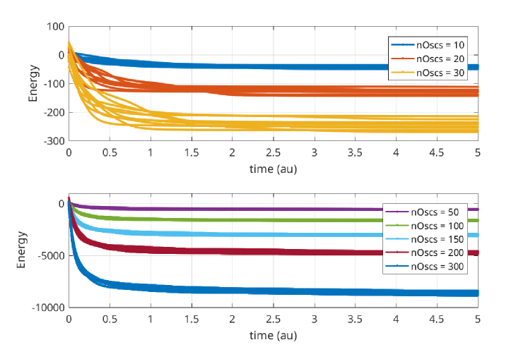
Figure 2: Energy vs.time for fully connected oscillator networks.

Furthermore, we fix the size of the network to 100 and vary the sparsity of the connections. The sparsity is defined as the ratio between the actual number of non-zero connections and the possible number of connections in a full network. Again, with each sparsity, 10 random samples are simulated; we plot the energy functions in Figure 3. From it, we see that with a fixed size, as the network gets sparser, the objective energy becomes shallower, and the convergence rate decreases marginally.

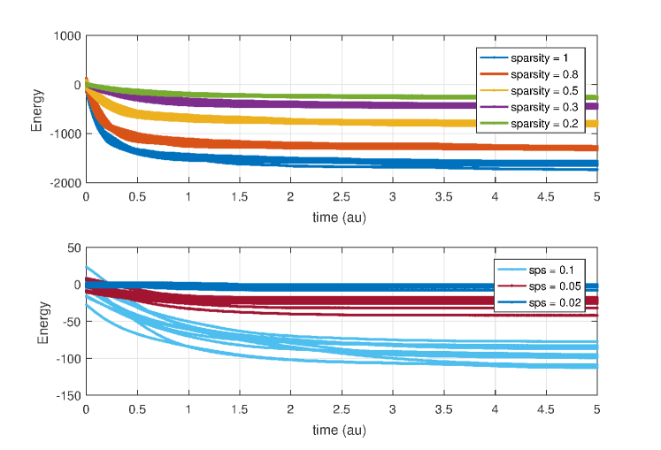
Figure 3: Energy vs.time for sparse oscillator networks.

In a fully connected network, both the average and largest distances between oscillators are $1$. In sparse random graphs, the largest distance, aka, the diameter, increases very marginally as the network becomes sparser [39]. Since the convergence rate in both cases does not change much with size or sparsity, it is natural to suspect that it may instead scale with the average or maximum distance between oscillators in the network. To study this possibility, we conduct further experiments and simulate the “worse case” for connection distance — all oscillators coupled are in a single line. In this case, both the average and largest distances grow linearly with the number of oscillators. From the energy functions plotted in Figure 4, we observe that even in this connection configuration, the speed does not change much with increased network size. These results are encouraging. As the problem size grows, the hardware size does need to increase [2], but the computation time remains almost constant.

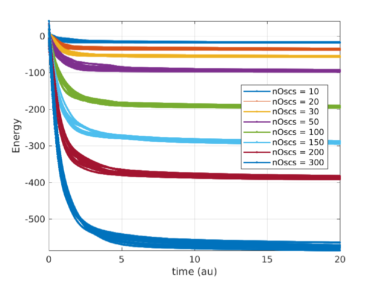
Figure 4: Energy vs.time for oscillators coupled in a single line.

Note that in all these results from the Kuramoto model, time is measured in seconds. The results are based on the Kuramoto model defined 13, where we assume $\omega_{0}=1$. In fact, from 10 we can see that the run time is inversely proportional to the product of $\omega_{0}$ and $A_{c}$. This is to say, if the oscillator’s frequency is at GHz scale, the time to synchronize becomes nanoseconds as opposed to seconds. Of course, for nano-oscillators, the coupling strength $A_{c}$ is normally not uniformly distributed between 0 and 1, as we have assumed in the results in this section. $A_{c}$ controls the number of cycles for the oscillators to synchronize; its value depends not only on the resistive coupling between oscillators, but also on the type of oscillator. As we show in Sec. IV, it may take LC oscillators coupled with $M\Omega$ resistors 100 cycles to synchronize their phases. Even so, it takes only a fraction of a microsecond for computation. While the speed is already appealing, employing other oscillator technologies can further improve it. Ring oscillators in standard CMOS technologies can nowadays achieve 100GHz, and are known to injection lock and synchronize quickly. Resonant Body Transistors (RBTs), a type of silicon-based CMOS-compatible MEMS resonators, have been demonstrated to achieve $>$10GHz frequency [40]. Spin-torque oscillators operate at frequencies of tens of GHz [41], offering exciting power and speed possibilities.

IV Examples

In this section, we demonstrate the feasibility of oscillator-based Ising machines with several examples.

IV-A Small MAX-CUT Problems

The MAX-CUT problem is a combinatorial optimization problem related to a graph, where we try to find a subset of vertices such that the total weights of the cut set between this subset and the remaining vertices are maximized. The MAX-CUT problem is one of Karp’s 21 NP-complete problems [42]. They have a direct mapping to the Ising model in 2, with $J_{ij}=J_{ji}$ representing the weight between node $i$ and node $j$. Then we can write the relationship between the Hamiltonian function and the cut size as

$$H=\sum_{i,j}J_{ij}s_{i}s_{j}=\sum_{i,j}J_{ij}-2S_{c},$$ (29)

where $S_{c}$ is the cut size — it is maximized when the Ising Hamiltonian is minimized.

We construct a small-sized MAX-CUT problem with a full graph of six vertices using the Kuramoto model in 13. Each edge has a random weight drawn from a uniform distribution between 0 and 2. The magnitude of SYNC is fixed at $A_{s}=2$, while we ramp up the coupling strength $A_{c}$ from 0 to 5. Results from the deterministic model ($A_{n}=0$) and the stochastic model ($A_{n}=0.1$) are shown in Figure 6 and Figure 6 respectively. In the plots, oscillators are started with random phases between 0 and $\pi$; after a while, they all settle to one of the two phase-locked states separated by $\pi$. These two groups of oscillators represent the two subsets of vertices in the solution. In this case, the results reliably return {2,3,6} and {1,4,5}. For this size-6 problem, we have enumerated all the possible cut sets — the result from phase-based simulation is indeed the global optimal solution.

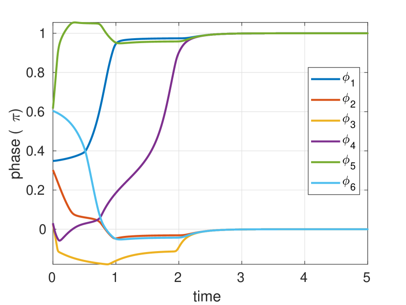
Figure 5: Phases of oscillators solving a size-6 MAX-CUT problem without noise.

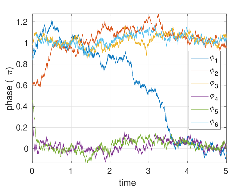
Figure 6: Phases of oscillators solving a size-6 MAX-CUT problem with noise.

The Kuramoto models are prototyped in a MATLAB${}^{\text{\textregistered}}$-based simulation platform MAPP [43, 44]. Here in the paper, we show the minimum code for generating the same results in Listings LABEL:lst:KuramotoF_sin and LABEL:lst:run_MAXCUT_6. Note that these are SDE simulations with random initial conditions. Every run will return different waveforms; there is no guarantee for achieving the ground state every time.

• ⬇

  1function fout = KuramotoF_sin(x, Ac, As, n, h, J)

  2 for c = 1:n

  3 fout(c, 1) = Ac * h(c) * sin(pi*x(c)) ...

  4 + Ac * J(c, :) * sin(pi*(x(c) - x));

  5 end

  6 fout = (fout - As * sin(2*pi*x))/pi;

  7end

  Listing 1: KuramotoF_sin.m

• ⬇

  1nOsc = 6;

  2h = zeros(nOsc, 1);

  3J = [ 0 0.9294 0.1682 0.2574 0.1395 0.3284

  4 0.9294 0 0.8639 0.8428 1.0879 0.0015

  5 0.1682 0.8639 0 1.2203 1.3125 0.0177

  6 0.2574 0.8428 1.2203 0 0.8108 0.5174

  7 0.1395 1.0879 1.3125 0.8108 0 1.6862

  8 0.3284 0.0015 0.0177 0.5174 1.6862 0];

  9

  10tstop = 5; tstep = 1e-3;

  11As = 2; Ac = 5; An = 0.1;

  12F = @(t,X) KuramotoF_sin(X, Ac*t/tstop, As, nOsc, h, J);

  13G = @(t,X) An*eye(nOsc);

  14

  15obj = sde(F, G, ’StartState’, rand(nOsc, 1));

  16[S, T] = simulate(obj, tstop/tstep, ’DeltaTime’, tstep);

  17

  18figure; plot(T, S);

  19legend(’\phi_1’, ’\phi_2’, ’\phi_3’, ...

  20 ’\phi_4’, ’\phi_5’, ’\phi_6’);

  21xlabel(’time’); ylabel(’phase (\pi)’);

  22box on; grid on;

  Listing 2: run_MAXCUT_6.m

Instead of using phase macromodels, we can also directly simulate oscillators’ DAEs as in 3 and achieve the same results. Such simulations are at a lower lever than macromodels and less efficient. But they are closer to physical reality and are standard in circuit design. In the simulations, six cross-coupled LC oscillators are tuned to a frequency of 1GHz. Each pair of oscillators $i$ and $j$ are coupled through a resistor with conductance $G_{0}\cdot J_{ij}$ between the opposite differential nodes, where $G_{0}=1/1M\Omega$. In this way, a positive resistor tends to develop opposite phases in the two oscillators, same as the effect of a positive $J_{ij}$ in the Ising Hamiltonian. Results from transient simulation using ngspice-26 are shown in Figure 7. The six oscillators’ phases settle into the correct two groups {2,3,6} and {1,4,5} within 0.1$\mu$s, which is about 100 cycles of oscillation. We have tried this experiment with different sets of random weights, starting from different random initial conditions; SPICE simulations on oscillators’ DAEs reliably return the optima of various size-6 MAX-CUT problems.

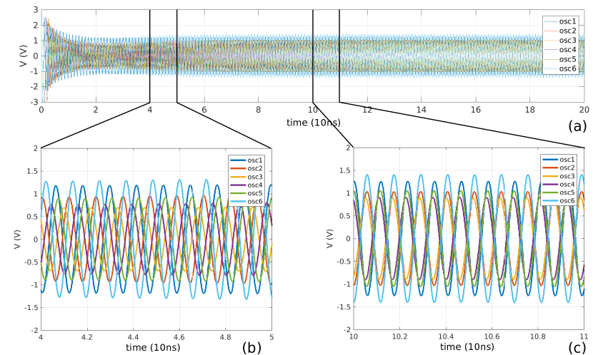
Figure 7: Simulation results from ngspice on 6 coupled oscillators.

On a breadboard, we implement an even smaller MAX-CUT problem by coupling four LC oscillators together. The CMOS devices are implemented with chips ALD1106/7. The inductors are of size 10mH; capacitors are 68nF. The central frequency is about 38kHz. And the potentiometers are of maximum resistance of 220kOhm. By tweaking the six potentiometers, we can conveniently adjust the edge weights to try various size-4 MAX-CUT problems. The results are observed using a four channel oscilloscope, as shown in Figure 8 (c). Through experiments with various sets of weights, we have validated that this is indeed a proof of concept hardware implementation of oscillator-based Ising machines, the first of its kind.

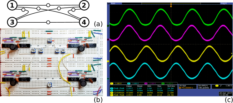
Figure 8: A simple oscillator-based Ising machine solving size-4 MAX-CUT problems: (a) illustration of the 6 connections of 4 units; (b) breadboard implementation with 4 CMOS LC oscillators and 6 potentiometers; (c) oscilloscope measurements showing the maximum cut is between nodes {1, 2} and {3, 4}.

IV-B A Larger MAX-CUT Problem

In this section, we test the proposed scheme on a larger-sized benchmark MAX-CUT — G22 from [45]. The graph has 2000 vertices and 19990 edges. We perform phase macromodel simulations with 2000 coupled oscillators, starting from random initial phases. In the process, we pump up the coupling strength $A_{c}$ while keeping the noise level $A_{n}$ constant. Instead of keeping the coupling from SYNC $A_{s}$ also constant, we find that ramping it up and down improves the results. Figure 9 Shows how the phases evolve over time. The corresponding cut size is plotted in Figure 10. The code for generating the results is shown in Listing LABEL:lst:KuramotoF and LABEL:lst:run_MAXCUT_G22. We have run the experiments with the same parameters 100 times; the mean and maximum cut sizes are shown in Table I.

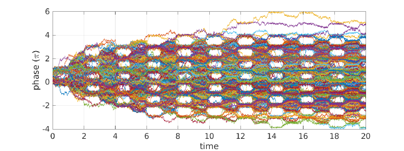
Figure 9: Phases of oscillators solving the G22 MAX-CUT benchmark problem [45].

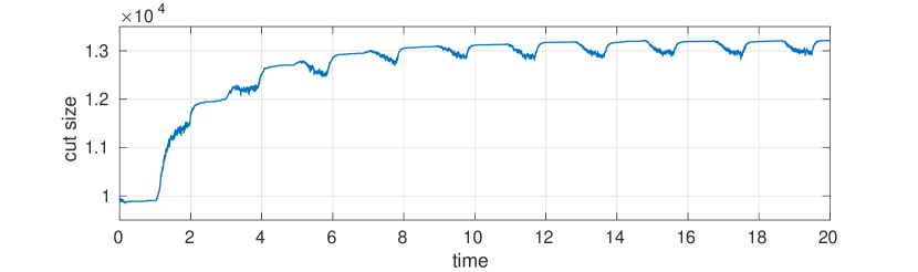
Figure 10: Cut size vs.time corresponding to results in Figure 9.

• ⬇

  1function fout = KuramotoF(x, Ac, As, n, h, J)

  2 k = 10; % sharpness of square wave

  3 for c = 1:n

  4 fout(c, 1) = Ac * h(c) * tanh(k*sin(pi*x(c))) ...

  5 + Ac * J(c, :) * tanh(k*sin(pi*(x(c) - x))) ...

  6 - As * sin(2*pi*x(c));

  7 end

  8 fout = fout/pi;

  9end

  Listing 3: KuramotoF.m

• ⬇

  1nOsc = 2000;

  2h = zeros(nOsc, 1);

  3G22 = importdata(’wherever_set1_is/g22.rud’, ’ ’, 1);

  4p = G22.data(:,1);

  5n = G22.data(:,2);

  6w = G22.data(:,3);

  7J = sparse(p, n, w, nOsc, nOsc);

  8J = J + J.’;

  9

  10An = 0.5; Ac = 8;

  11tstop = 20; tstep = 5e-3;

  12

  13a1.k = Ac/tstop;

  14f1 = @(t, args) t*args.k;

  15

  16a2.T = tstop/10;

  17f2 = @(t, args) 4+6*tanh(10*cos(2*pi*t/args.T));

  18

  19F = @(t,X) KuramotoF(X, f1(t, a1), f2(t, a2), nOsc,h,J);

  20G = @(t,X) An*eye(nOsc);

  21

  22obj = sde(F, G, ’StartState’, rand(nOsc, 1));

  23[S, T] = simulate(obj, tstop/tstep, ’DeltaTime’, tstep);

  24

  25figure; plot(T, S); box on; grid on;

  26

  27Es = T;

  28for k = 1:length(T)

  29 ix = find(mod(round(S(k,:)), 2));

  30 Es(k) = sum(sum(J(ix, setdiff(1:nOsc, ix))));

  31end

  32figure; plot(T, Es);

  Listing 4: run_MAXCUT_G22.m

	mean in 100	best in 100
CIM[11]	13248	13313
our scheme	13253	13305
without noise	13203	13249
without SYNC	13050	13155
sinusoidal PPV	13214	13276
1% var. in freq.	13249	13309
5% var. in freq.	13252	13303

TABLE I: Results of oscillator-based Ising machines with different configurations run on MAX-CUT benchmark G22, compared with coherent Ising machine (CIM) [11].

More experiments have been conducted on this benchmark to demonstrate the mechanism of oscillator-based Ising machines. We have tried removing noise from the model, i.e., $A_{n}=0$; the solutions are considerably worse, as shown in Table I. We have also tried this Ising machine without SYNC, i.e., changing f2 in Listing LABEL:lst:run_MAXCUT_G22 to always return 0. Then the coupled oscillators become the same as an associative memory array people use for specialized image processing tasks [21, 22, 23]. As shown in Table I, we have observed significantly worse results from such coupled-oscillator-based associative memories. SYNC and the mechanism of SHIL are indeed essential in the operation of oscillator-based Ising machines.

Moreover, in Listing LABEL:lst:KuramotoF, we have changed the Kuramoto model, making the $\sin()$ term in 10 a smooth square function. This changes the $\cos()$ term in the energy function 14 to a triangle function. Such a change appears to give better results than the original. It requires designing oscillators with special PPVs and waveforms such that the convolution of them is a square wave, e.g., oscillators with square PPVs and spiky waveforms, or vice versa. This is not difficult in practice. In fact, rotary traveling wave oscillators naturally have square PPVs [46]. Ring oscillators can also be designed with various PPVs and waveforms by sizing each stage individually. The best phase macromodel with the optimal energy function for oscillator-based Ising machines is yet to be studied. But whatever it may be, oscillators are versatile enough to be designed with the desired properties.

We can also assume there is some variability in the central frequencies of oscillators. In Listing LABEL:lst:KuramotoF, we show results from simulating equation 20, with $\Delta\omega_{i}$ from a Gaussian distribution, generated by randn(2000, 1) * 0.01 and randn(2000, 1) * 0.05 in MATLAB${}^{\text{\textregistered}}$. Even with such non-trivial variations in the central frequencies of oscillators, the performances do not seem to be affected.

IV-C A Boolean Logic Example: Half Adder

As mentioned in Sec. I, we can design the Ising Hamiltonian such that its ground states encode the solutions of a logic circuit. Then Ising machines can be used to perform invertible Boolean logic computation [14, 3]. In this section, we illustrate this capability with a simple example. We design a small Ising machine that encodes the logic of an adder.

$$a+b=2c+s,$$ (30)

where $s$ is the sum and $c$ is the carry bit; all variables are binary, i.e., $a,b,c,s\in\{0,~{}1\}$.

The Ising Hamiltonian can be formulated as follows.

$$H =(a+b-2c-s)^{2}$$

$$=a^{2}+b^{2}+4c^{2}+s^{2}+2ab-4ac-2as-4bc-2bs+4cs$$

$$=a+b+4c+s+2ab-4ac-2as-4bc-2bs+4cs,$$ (31)

where we have used the equality $a^{2}=a$ for binary variables. Such a Hamiltonian function is by definition greater than or equal to zero, and only reaches zero when the relationship in 30 is satisfied.

We can rewrite the Ising Hamiltonian in a similar format as 1.

$$H=\vec{h}_{x}^{T}\cdot\vec{x}+x^{T}\cdot\mathbf{J}\cdot x,$$ (32)

where

$$\vec{x} =[c,~{}s,~{}a,~{}b]^{T},$$ (33)

$$\vec{h}_{x} =[4,~{}1,~{}1,~{}1]^{T},$$ (34)

$$\mathbf{J} =\left[\begin{array}[]{cccc}0&2&-2&-2\\ 2&0&-1&-1\\ -2&-1&0&1\\ -2&-1&1&0\end{array}\right].$$ (39)

To match the definition in 1, we can convert binary variables $a,b,c,s$ from $\{0,~{}1\}$ to $\{-1,~{}+1\}$ by defining $\vec{s}=2\vec{x}-1$. Then we have

$$H=\vec{h}^{T}\cdot\vec{s}+s^{T}\cdot\mathbf{J}\cdot s+Const,$$ (40)

where

$$\vec{h}=\vec{h}_{x}-\text{sum}(\mathbf{J},~{}2)=[2,~{}1,~{}-1,~{}-1]^{T},$$ (41)

with the same $\mathbf{J}$ as in 39.

When this Ising machine settles to the ground state, variables $a,b,c,s$ will satisfy the adder relationship in 30. Therefore, if we fix the value of $a$ and $b$, the $c$ and $s$ values we read from the results will be the carry and sum from the adder circuit. On the other hand, if $c$ or $s$ is fixed, $a$ and $b$ will settle to values that solve for the adder relationship. These predictions can be verified by transient simulation results shown in Figure 12 and Figure 12, generated by the script in Listing LABEL:lst:run_half_adder.

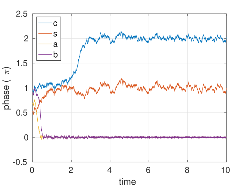
Figure 11: Phase-based half adder ($a+b=2c+s$) with $a=1$, $b=1$. Result here shows $c=1(2\pi)$, $s=0(\pi)$.

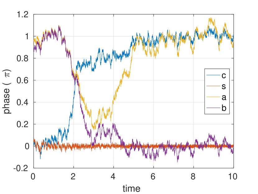
Figure 12: Phase-based half adder ($a+b=2c+s$) with $s=1$. Result here shows $c=0$, $a=0$, $b=1$.

• ⬇

  1nOsc = 4;

  2

  3% h = [2;1;-1;-1]; % does not pin anything

  4% h = [2;1;-100;-100]; % pin a=1, b=1

  5% h = [-100;1;-1;-1]; % pin c to logic 1

  6h = [2;-100;-1;-1]; % pin s to logic 1

  7

  8J = [0 2 -2 -2

  9 2 0 -1 -1

  10 -2 -1 0 1

  11 -2 -1 1 0];

  12

  13tstop = 10; tstep = 1e-3;

  14

  15Ac = 5; An = 0.1; As = 2;

  16F = @(t,X) KuramotoF_sin(X, Ac*t/tstop, As, nOsc, h, J);

  17G = @(t,X) An*eye(nOsc);

  18

  19obj = sde(F, G, ’StartState’, rand(nOsc, 1));

  20[S, T] = simulate(obj, tstop/tstep, ’DeltaTime’, tstep);

  21

  22figure; plot(T, S);

  23legend(’c’, ’s’, ’a’, ’b’);

  24xlabel(’time’); ylabel(’phase (\pi)’);

  25box on; grid on;

  Listing 5: run_half_adder.m

Note that for larger problems, Ising machines normally settle to local optima. While local optima are often good enough for combinatorial optimization, they can be meaningless for invertible Boolean logic problems. Therefore, the suitability of applying Ising machines to logic problems still needs more study.

Conclusion

In this paper, we proposed schemes for implementing Ising machines using self-sustaining nonlinear oscillators. We have conducted a comprehensive study of their mechanism, from oscillator DAEs to the phase macromodel, then to the “energy” represented by the Lyapunov function and its relationship with the Ising Hamiltonian, finally to the use of Boltzmann law and annealing profiles to achieve better minima. We have also studied the effect of variations, where our scheme has potential advantages over existing ones thanks to its use of self-sustaining oscillators and phase-based logic encoding. We also showed that the computation time for oscillator-based Ising machines stays mostly constant as problem size grows, and is dependent mainly on the oscillator technology. Finally, the validity and feasibility of the scheme are examined by multiple levels of simulation and proof of concept hardware implementation. Simulations run on benchmark combinatorial optimization problems show promising results, matching the state of art in the development of practical Ising machines.

References

- [1] E. Ising. Beitrag zur theorie des ferromagnetismus. Zeitschrift für Physik A Hadrons and Nuclei, 31(1):253–258, 1925.
- [2] A. Lucas. Ising formulations of many NP problems. arXiv preprint arXiv:1302.5843, 2013.
- [3] M. Gu and Á. Perales. Encoding universal computation in the ground states of Ising lattices. Physical Review E, 86(1):011116, 2012.
- [4] M. W. Johnson, M. H. S. Amin, S. Gildert, T. Lanting, F. Hamze, N. Dickson, R. Harris, A. J. Berkley, J. Johansson, P. Bunyk and others. Quantum Annealing with Manufactured Spins. Nature, 473(7346):194, 2011.
- [5] Z. Bian, F. Chudak, R. Israel, B. Lackey, W. G. Macready and A. Roy. Discrete optimization using quantum annealing on sparse Ising models. Frontiers in Physics, 2:56, 2014.
- [6] R. Harris, J. Johansson, A. J. Berkley, M. W. Johnson, T. Lanting, S. Han, P. Bunyk, E. Ladizinsky, T. Oh, I. Perminov and others. Experimental Demonstration of a Robust and Scalable Flux Qubit. Physical Review B, 81(13):134510, 2010.
- [7] T. F. Rønnow, Z. Wang, J. Job, S. Boixo, S. V. Isakov, D. Wecker, J. M. Martinis, D. A. Lidar and M. Troyer. Defining and detecting quantum speedup. Science, 345(6195):420–424, 2014.
- [8] V. S. Denchev, S. Boixo, S. V. Isakov, N. Ding, R. Babbush, V. Smelyanskiy, J. Martinis, H. Neven. What is the computational value of finite-range tunneling? Physical Review X, 6(3):031015, 2016.
- [9] A. Marandi, Z. Wang, K. Takata, R. L. Byer and Y. Yamamoto. Network of time-multiplexed optical parametric oscillators as a coherent Ising machine. Nature Photonics, 8(12):937–942, 2014.
- [10] P. L. McMahon, A. Marandi, Y. Haribara, R. Hamerly, C. Langrock, S. Tamate and T. Inagaki, H. Takesue, S. Utsunomiya, K. Aihara and others. A fully-programmable 100-spin coherent Ising machine with all-to-all connections. Science, page aah5178, 2016.
- [11] T. Inagaki, Y. Haribara, K. Igarashi, T. Sonobe, S. Tamate, T. Honjo, A. Marandi, P. L. McMahon, T. Umeki, K. Enbutsu and others. A coherent Ising machine for 2000-node optimization problems. Science, 354(6312):603–606, 2016.
- [12] I. Mahboob, H. Okamoto and H. Yamaguchi. An electromechanical Ising Hamiltonian. Science Advances, 2(6):e1600236, 2016.
- [13] B. Sutton, K. Y. Camsari, B. Behin-Aein and S. Datta. Intrinsic optimization using stochastic nanomagnets. Scientific Reports, 7, 2017.
- [14] K. Y. Camsari, R. Faria, B. M. Sutton and S. Datta. Stochastic p-Bits for Invertible Logic. Physical Review X, 7(3):031014, 2017.
- [15] M. Yamaoka, C. Yoshimura, M. Hayashi, T. Okuyama, H. Aoki and H. Mizuno. A 20k-spin Ising Chip to Solve Combinatorial Optimization Problems with CMOS Annealing. IEEE Journal of Solid-State Circuits, 51(1):303–309, 2016.
- [16] A. Neogy and J. Roychowdhury. Analysis and Design of Sub-harmonically Injection Locked Oscillators. In Proc. IEEE DATE, Mar 2012. DOI link.
- [17] T. Wang and J. Roychowdhury. Design Tools for Oscillator-based Computing Systems. In Proc. IEEE DAC, pages 188:1–188:6, 2015. DOI link.
- [18] T. Wang. Sub-harmonic Injection Locking in Metronomes. arXiv preprint arXiv:1709.03886, 2017.
- [19] T. Wang and J. Roychowdhury. PHLOGON: PHase-based LOGic using Oscillatory Nanosystems. In Proc. UCNC, LNCS sublibrary: Theoretical computer science and general issues. Springer, July 2014. DOI link.
- [20] J. Roychowdhury. Boolean Computation Using Self-Sustaining Nonlinear Oscillators. Proceedings of the IEEE, 103(11):1958–1969, Nov 2015. DOI link.
- [21] F. Hoppensteadt and E. Izhikevich. Synchronization of laser oscillators, associative memory, and optical neurocomputing. Physical Review E, 62(3):4010, 2000.
- [22] P. Maffezzoni, B. Bahr, Z. Zhang and L. Daniel. Oscillator array models for associative memory and pattern recognition. IEEE Trans. on Circuits and Systems I: Fundamental Theory and Applications, 62(6):1591–1598, June 2015.
- [23] M. Pufall, W. Rippard, G. Csaba, D. Nikonov, G. Bourianoff and W. Porod. Physical Implementation of Coherently Coupled Oscillator Networks. IEEE Journal on Exploratory Solid-State Computational Devices and Circuits, 1:76–84, 2015.
- [24] F. C. Hoppensteadt and E. M. Izhikevich. Weakly Connected Neural Networks, volume 126. Springer Science & Business Media, 2012.
- [25] S. Kim, S. H. Park and C. S. Ryu. Multistability in Coupled Oscillator Systems with Time Delay. Physical review letters, 79(15):2911, 1997.
- [26] A. Demir, A. Mehrotra, and J. Roychowdhury. Phase Noise in Oscillators: a Unifying Theory and Numerical Methods for Characterization. IEEE Trans. Ckts. Syst. – I: Fund. Th. Appl., 47:655–674, May 2000. DOI link.
- [27] X. Lai and J. Roychowdhury. Capturing injection locking via nonlinear phase domain macromodels. IEEE Trans. Microwave Theory Tech., 52(9):2251–2261, September 2004. DOI link.
- [28] R. Adler. A study of locking phenomena in oscillators. Proc. IEEE, 61:1380–1385, 1973. Reprinted from [47].
- [29] J. A. Acebrón, L. L. Bonilla, C. J. P. Vicente, F. Ritort and R. Spigler. The Kuramoto Model: A Simple Paradigm for Synchronization Phenomena. Reviews of Modern Physics, 77(1):137, 2005.
- [30] P. Bhansali and J. Roychowdhury. Gen-Adler: The generalized Adler’s equation for injection locking analysis in oscillators. In Proc. IEEE ASP-DAC, pages 522–227, January 2009. DOI link.
- [31] S. Smale. On Gradient Dynamical Systems. Annals of Mathematics, pages 199–206, 1961.
- [32] L. D. Landau and E. M. Lifshitz. Statistical Physics: V. 5: Course of Theoretical Physics. Pergamon press, 1969.
- [33] R. Yuan, Y. Ma, B. Yuan and P. Ao. Constructive Proof of Global Lyapunov Function as Potential Function. arXiv preprint arXiv:1012.2721, 2010.
- [34] A. Jadbabaie, N. Motee and M. Barahona. On the stability of the Kuramoto Model of Coupled Nonlinear Oscillators. In Proceedings of the American Control Conference, volume 5, pages 4296–4301. IEEE, 2004.
- [35] Y. Wang and F. J. Doyle. Exponential Synchronization Rate of Kuramoto oscillators in the Presence of a Pacemaker. IEEE Transactions on Automatic Control, 58(4):989–994, 2013.
- [36] F. Dörfler and F. Bullo. Synchronization in Complex Networks of Phase Oscillators: A Survey. Automatica, 50(6):1539–1564, 2014.
- [37] S. K. Patra and A. Ghosh. Statistics of Lyapunov exponent spectrum in randomly coupled Kuramoto oscillators. Physical Review E, 93(3):032208, 2016.
- [38] T. Coletta, R. Delabays and P. Jacquod. Finite-size Scaling in the Kuramoto Model. Physical Review E, 95(4):042207, 2017.
- [39] F. Chung and L. Lu. The diameter of Sparse Random Graphs. Advances in Applied Mathematics, 26(4):257–279, 2001.
- [40] D. Weinstein and S. A. Bhave. The Resonant Body Transistor. Nano letters, 10(4):1234–1237, 2010.
- [41] M. R. Pufall, W. H. Rippard, S. Kaka, T. J. Silva, and S. E. Russek. Frequency modulation of spin-transfer oscillators. Applied Physics Letters, 86(8):082506–+, February 2005.
- [42] R. M. Karp. Reducibility among combinatorial problems. In Complexity of computer computations, pages 85–103. Springer, 1972.
- [43] T. Wang, K. Aadithya, B. Wu, J. Yao, and J. Roychowdhury. MAPP: The Berkeley Model and Algorithm Prototyping Platform. In Proc. IEEE CICC, pages 461–464, September 2015. DOI link.
- [44] T. Wang, A. V. Karthik, B. Wu and J. Roychowdhury. MAPP: A platform for prototyping algorithms and models quickly and easily. In IEEE MTT-S International Conference on Numerical Electromagnetic and Multiphysics Modeling and Optimization (NEMO), pages 1–3. IEEE, 2015.
- [45] P. Festa, P. M. Pardalos, M. G. C. Resende, and C. C. Ribeiro. Randomized heuristics for the MAX-CUT problem. Optimization methods and software, 17(6):1033–1058, 2002.
- [46] Y. Chen and K. D. Pedrotti. Rotary traveling-wave oscillators, analysis and simulation. IEEE Transactions on Circuits and Systems I: Regular Papers, 58(1):77–87, 2011.
- [47] R. Adler. A study of locking phenomena in oscillators. Proceedings of the I.R.E. and Waves and Electrons, 34:351–357, June 1946. Reprinted as [28].