Optimizing Quantum Models of Classical Channels:
The reverse Holevo problem

Optimizing Quantum Models of Classical Channels:
The reverse Holevo problem

Abstract

Given a classical channel—a stochastic map from inputs to outputs—the input can often be transformed to an intermediate variable that is informationally smaller than the input. The new channel accurately simulates the original but at a smaller transmission rate. Here, we examine this procedure when the intermediate variable is a quantum state. We determine when and how well quantum simulations of classical channels may improve upon the minimal rates of classical simulation. This inverts Holevo’s original question of quantifying the capacity of quantum channels with classical resources. We also show that this problem is equivalent to another, involving the local generation of a distribution from common entanglement.

I Introduction

One speaks of a quantum advantage when a computational task is performed more efficiently (in memory, time, or both) using quantum mechanical hardware than classical hardware. Quantum advantages appear in the simulation of a variety of classical systems [1]: thermal states [2], fluid flows [3, 4], electromagnetic fields [5], diffusion processes [6, 7], Burger’s equation [8], and molecular dynamics [9]. Quantum advantage also has been found in more mathematical contexts. The most well-known problems include the factorization of prime numbers (Shor’s integer factoring algorithm [10]), database search (Grover’s algorithm [11]), and the efficient solution of linear systems [12].

A recent but rich area of study is the quantum advantage for simulating classical stochastic processes. By stochastic process, we mean a source that probabilistically generates a sequence of symbols $x_{0}x_{1}\dots x_{t}$. When the probability of each new symbol $x_{t}$ depends on the previous symbols, the process is said to have memory. Computational mechanics has previously studied the memory resources required for simulating and predicting stochastic processes using classical hardware [13, 14, 15]. Quantum computational mechanics now proposes to use sequential measurements of a quantum system as a more resource-efficient means of simulating stochastic processes [16, 17, 18, 19, 20].

Recent efforts showed that many important results on optimal simulation and prediction do not carry over from the classical to the quantum domain. For instance, it is a common fact of resource theories that a given resource (say, memory) may have various inequivalent quantifications depending on the specific task at hand (say, asymptotic rates versus single-shot requirements). In classical computational mechanics, in contrast, a stochastic process has a uniquely optimal predictive model—the $\epsilon$-machine. It is minimal according to all quantifications of memory. In this sense, the $\epsilon$-machine strongly minimizes memory [21]. However, this no longer holds for quantum models, where inequivalent quantifications have inequivalent minima. For example, a model that is optimal for single-shot implementations is not the optimal model for the asymptotic rate. We call this weak optimization [21, 22].

In a memoryful stochastic process, the future is dependent on the past through what is mathematically considered a probabilistic channel. This motivates the exploration of simulating classical channels with quantum resources, which is a fundamental question that sheds light on the more complicated problem of simulating stochastic processes. This question is the main motivator of the following development, although we call-out ancillary results along the way.

Simulating a classical channel with quantum resources is in many ways the inverse of much previous work on channels in quantum information. There, the focus is often on the resources (such as entanglement) required to simulate a fully quantum channel [23, 24, 25]. It also often addresses the capacity of a quantum channel to transmit classical information, first considered by Holevo [26, 27, 28, 29]. Rather than using classical capacities as a means to study the properties of quantum channels, the following uses quantum resources as a means to study the properties of purely classical channels. Thus, in the spirit of the “reverse Shannon theorem” [24], we consider this a reverse Holevo problem.

Our results also draw from the literature of common information [30, 31], which concerns simulating channels with intermediate classical variables. We adapt those results to the quantum domain by making the intermediate variable quantal.

The following (second) section establishes notation and definitions for our development. The third presents our three main results for the reverse Holevo problem:

1. For every channel, there are quantum models that reduce memory costs across all quantifications of memory (or, in rare cases, do at least as well as the original channel).

2. However, there is generally not a single quantum model that is minimal with respect to all quantifications of memory. This has important implications for single-shot channel simulation.

3. We demonstrate a lower bound for the asymptotic cost of modeling a channel with quantum resources.

We also present a mathematical correspondence between the reverse Holevo problem and another that we call common entanglement. The latter asks for the entanglement cost of generating a bivariate classical distribution using only entanglement and local operations (without communication). This correspondence sets the stage for further developments.

II Notation and definitions

This section adapts results from computational mechanics, as well as from the theory of common information, to describe Shannon communication channels.

Computational mechanics is a subfield of statistical mechanics that addresses the information-theoretic and energetic costs of simulating and predicting stochastic processes [15, 32]. In that setting, a stochastic process is defined by an alphabet $\mathcal{A}$ and a probability measure $\mathbb{P}\left(x_{-\infty:\infty}\right)$ over all bi-infinite words $x_{-\infty:\infty}=\dots x_{-1}x_{0}x_{1}\dots$ such that $x_{t}\in\mathcal{A}$ for all $t\in\mathbb{Z}$.

Random variables are denoted by capital Latin letters $X$, $Y$, and so on, and their outcomes by $x\in\mathcal{X}$, $y\in\mathcal{Y}$, and so on. The calligraphic letters $\mathcal{X},\mathcal{Y}$, and so on represent finite sets.

Classical distributions are denoted by $\mathbb{P}$. For example, the probability of a random variable $X$ taking value $x\in\mathcal{X}$ is given by $\mathbb{P}(X=x)$ if the random variable needs to be specified and is shortened to $\mathbb{P}(x)$ if it can be inferred from context. We say $Y=f(X)$ for a function $f:\mathcal{X}\rightarrow\mathcal{Y}$ if $\mathbb{P}\left(Y=y\right)=\sum_{x:f(x)=y}\mathbb{P}\left(X=x\right)$.

As a measure of its information content, the uncertainty of a random variable is measured by its Rényi entropies:

$$H_{\alpha}\left(X\right):=\frac{1}{1-\alpha}\log\left(\sum_{x\in\mathcal{X}}\mathbb{P}(x)^{\alpha}\right)~{},$$

for $\alpha\in(0,1)$ and $\alpha\geq 1$. In the limits $\alpha\rightarrow 0$ and $\alpha\rightarrow 1$, we recover the max-entropy $H_{0}\left(X\right):=\log\left|\mathcal{X}\right|$ (useful for costs in single-shot or zero-error situations) and the Shannon entropy $H(X):=-\sum_{x}\mathbb{P}(x)\log\mathbb{P}(x)$, respectively. An important property of the Rényi entropies is that they are monotonically decreasing under the application of a deterministic function. That is, if $Y=f(X)$, then $H(Y)\leq H(X)$, with equality only when $f$ is bijective.

II.1 Classical channels

When discussing channels, we consider an input space $\mathcal{X}$ and output space $\mathcal{Y}$, both (for convenience) assumed to be discrete. On these one may define random variables $X$ and $Y$, respectively. A channel $\mathcal{C}$ is then a conditional probability function $\mathbb{P}_{\mathcal{C}}\left(Y=y\middle|X=x\right)$, which for each outcome $x\in\mathcal{X}$ in the input space defines a probability distribution over the output space $\mathcal{Y}$. We write such a channel as $\mathcal{C}:\mathcal{X}\rightsquigarrow\mathcal{Y}$, distinguishing it from a function via the squiggly arrow.

When it comes to information theory, a channel’s associated costs and resources depend on the input distribution $\mathbb{P}\left(X=x\right)$. One may vary these inputs to determine maximum capacities or minimum costs, for example. When speaking of a channel $\mathcal{C}$, though, for completeness we assume that an input distribution has been defined and so $XY$ forms a bivariate random variable. $XY$ is defined on the space $\mathcal{X}\times\mathcal{Y}$ with probability distribution $\mathbb{P}\left(X=x,Y=y\right)=\mathbb{P}_{\mathcal{C}}\left(Y=y\middle|X=x\right)\mathbb{P}\left(X=x\right)$. This assumption does not affect the generality of our results.

For bivariate random variables, the Shannon entropy can be used to define the conditional entropies and mutual information:

$$H\left(X\middle|Y\right) :=H\left(XY\right)-H\left(Y\right)~{},$$

$$H\left(X\middle|Y\right) :=H\left(XY\right)-H\left(Y\right)~{},~{}\text{and}$$

$$I\left(X:Y\right) :=H\left(X\right)+H\left(Y\right)-H\left(XY\right)~{}.$$

These represent the uncertainty remaining in $X$ when $Y$ is known, the uncertainty in $Y$ when $X$ is known, and the information shared between $X$ and $Y$, respectively.

We wish to simulate a particular channel $\mathcal{C}$. That is, we want (i) a random variable $Z$ defined on an intermediate space $\mathcal{Z}$, (ii) an encoding channel $\mathcal{E}:\mathcal{X}\rightarrow\mathcal{Z}$ with conditional distribution $\mathbb{P}_{\mathcal{E}}\left(Z=z\middle|X=x\right)$, and (iii) a decoding channel $\mathcal{D}:\mathcal{Z}\rightsquigarrow\mathcal{Y}$ with conditional distribution $\mathbb{P}_{\mathcal{D}}\left(Y=y\middle|Z=z\right)$ such that:

$$\mathbb{P}_{\mathcal{C}}\left(y\middle|x\right)=\sum_{z\in\mathcal{Z}}\mathbb{P}_{\mathcal{D}}\left(y\middle|z\right)\mathbb{P}_{\mathcal{E}}\left(z\middle|x\right)~{}.$$

We write this composition rule as $\mathcal{C}=\mathcal{D}\circ\mathcal{E}$. We call the triplet $M=\left(\mathcal{Z},\mathcal{E},\mathcal{D}\right)$ a model of channel $\mathcal{C}$.

Additionally, $X-Z-Y$ form a Markov chain. The data processing inequality tells us that $H(Z)\geq I\left(X:Z\right)\geq I\left(X:Y\right)$. This puts a constraint on models that simulate a given channel $\mathcal{C}$.

It is helpful to consider a particular subset of models called factorizations or, simply, factors. These are triples $F=\left(\mathcal{Z},f,\mathcal{D}\right)$, where the encoder is a deterministic function $f:\mathcal{X}\rightarrow\mathcal{Z}$.

Factors and models may be visualized by the commuting diagram of Fig. 1.

Figure 1: Information flow when simulating a channel: When $(\mathcal{Z},\mathcal{E},\mathcal{D})$ is a model, all paths in the diagram from $X$ to $Y$ represent the same channel—the diagram commutes. When $\mathcal{E}=f$ is a deterministic function, the model is a factor.

What is the use of a model or a factor? Their use arises when considering channels as a resource. If we do not have access to a physical system that directly implements channel $\mathcal{C}$, we may resort to systems that instead implement channels $\mathcal{E}$ and $\mathcal{D}$ in a model $M=\left(\mathcal{Z},\mathcal{E},\mathcal{D}\right)$ of $\mathcal{C}$. The more information required to store the intermediate variable $Z$, the more “costly” the model.

Models may be compared in quantifiable terms—through measurable features, such as the Rényi entropies of the intermediate variable $Z$—or they may be compared operationally. On the quantifiable side, one may pick a particular value of $\alpha$ and ask which model has the larger $H_{\alpha}\left(Z\right)$. Given two models $M_{1}=(\mathcal{Z}_{1},\mathcal{E}_{1},\mathcal{D}_{1})$ and $M_{2}=(\mathcal{Z}_{2},\mathcal{E}_{2},\mathcal{D}_{2})$ one often finds that $M_{1}$ is advantageous with respect to some $\alpha$—$H_{\alpha}\left(Z_{1}\right)\leq H_{\alpha}\left(Z_{2}\right)$—while $M_{2}$ is advantageous with respect to others—$H_{\alpha}\left(Z_{2}\right)\leq H_{\alpha}\left(Z_{1}\right)$.

Sometimes, however, the advantage of $M_{1}$ over $M_{2}$ is unilateral. Given two models $M_{1}$ and $M_{2}$ of a channel $\mathcal{C}$, we say that $M_{1}$ is strongly advantageous with respect to $M_{2}$ if, for all $\alpha\geq 0$, $H_{\alpha}\left(Z_{1}\right)\leq H_{\alpha}\left(Z_{2}\right)$.

This differs from being strictly advantageous, which implies for at least one $\alpha$ we have $H_{\alpha}\left(Z_{1}\right)<H_{\alpha}\left(Z_{2}\right)$ without equality.

In contrast, the operational approach asks whether one model of a channel $\mathcal{C}$ can effectively substitute for another. For factorizations, there is a particularly useful operational comparison: given factorizations $F_{1}=(\mathcal{Z}_{1},f_{1},\mathcal{D}_{1})$ and $F_{2}=(\mathcal{Z}_{2},f_{2},\mathcal{D}_{2})$ of channel $\mathcal{C}$, we say that $F_{2}$ is sufficient for $F_{1}$ if there is a deterministic function $g:\mathcal{Z}_{2}\rightarrow\mathcal{Z}_{1}$ such that Fig. 2’s diagram commutes.

Figure 2: Channel sufficiency: $F_{2}=(\mathcal{Z}_{2},f_{2},\mathcal{D}_{2})$ is sufficient for $F_{1}=(\mathcal{Z}_{1},f_{1},\mathcal{D}_{1})$ if, for some deterministic $g$, this diagram commutes.

The idea behind this comparison is that factorization $F_{2}$ itself can be factorized to yield the model $F_{1}$. In effect, $F_{2}$ already uses all the memory required to implement $F_{1}$, as well as some additional overhead. The takeaway, then, is that we might as well use $F_{1}$, as $F_{2}$ costs at least as much.

As a consequence of the concavity of Rényi entropies, the statement “$F_{2}$ is sufficient for $F_{1}$” necessarily implies that $F_{1}$ is strongly advantageous with respect to $F_{2}$. If $F_{2}$ is sufficient for $F_{1}$ and the function $g:\mathcal{Z}_{2}\rightarrow\mathcal{Z}_{1}$ is not bijective, then $F_{1}$ is strictly advantageous with respect to $F_{2}$.

Our focus on factorizations pays off with the following result from computational mechanics: For each channel $\mathcal{C}$, there exists a causal factorization $F_{\mathcal{C}}$, unique up to isomorphism, for which all other factorizations $F$ of $\mathcal{C}$ are sufficient [14]. Consequently, $F_{\mathcal{C}}$ is strongly minimal with respect to all other factorizations. The rule that $F_{\mathcal{C}}(x_{1})=F_{\mathcal{C}}(x_{2})$ if and only if $\mathbb{P}\left(Y=y\middle|X=x_{1}\right)=\mathbb{P}\left(Y=y\middle|X=x_{2}\right)$ defines $F_{\mathcal{C}}$ up to an isomorphism [13]. (As a consequence, the image of the factorization $Z_{\mathcal{C}}$ is the minimal sufficient statistic of $X$ with respect to $Y$.)

Notice, that the data processing inequality provides the lower bound $H\left(Z\right)\geq I\left(X:Y\right)$ for all models and factorizations of $\mathcal{C}$. This lower bound is generally not achievable with factorizations.

One might conjecture that the nonachievability of $I(X:Y)$ is a consequence of constraining our models to factorizations. However, the problem extends further. The more general problem of optimal models (in the broader, stochastic sense defined above) falls under the purview of common information theory [30, 31]. Common information refers to the problem of determining when a bivariate distribution $XY$ may be jointly generated from a common variable $Z$ by local stochastic maps. That is, if $Z$ is distributed according to $\mathbb{P}\left(Z=z\right)$, then $XY$ is distributed according to:

$$\mathbb{P}\left(x,y\right)=\sum_{z\in\mathcal{Z}}\mathbb{P}_{A}\left(x\middle|z\right)\mathbb{P}_{B}\left(y\middle|z\right)\mathbb{P}\left(z\right)$$

for channels $\mathbb{P}_{A}$ and $\mathbb{P}_{B}$. Any such joint generation scheme can be rewritten as a model of the channel $\mathcal{C}$ from $\mathcal{X}$ to $\mathcal{Y}$. In this way, results in the field of common information carry over to models of channels.

In particular, Wyner introduced a measure of common information that relates the asymptotic problem of modeling to the single-shot problem [30]. In the asymptotic regime, we can discuss a more general type of model. A $(n,M,\epsilon)$-model of $\mathcal{C}$ is a pair of channels $\mathcal{E}:X\rightarrow Z$ and $\mathcal{D}:Z\rightarrow Y$ such that $\mathcal{E}\left(X\right)$ is uniform over $M$ outcomes and:

$$\left\|\widehat{\mathbb{P}}\left(x,y\right)-\mathbb{P}(x,y)\right\|_{1}<\epsilon~{},$$

where $\widehat{\mathbb{P}}\left(x,y\right)=\mathbb{P}_{\mathcal{D}\circ\mathcal{E}}\left(y\middle|x\right)\mathbb{P}(x)$.

That is, $(n,M,\epsilon)$ is a model that approximates $n$ independent and identically distributed copies of the channel $\mathcal{C}$ with entropy cost $H(Z)=\log M$ and error $\epsilon$. Error here is measured by the $\ell^{1}$-norm $\left\|\cdot\right\|_{1}$. Wyner’s result, strengthened by Winter and Ahlswede [33, 34], is that for any $\epsilon,\delta>0$ there exists a sufficiently large $n$ such that an $(n,M,\epsilon)$ model is Markov with $\frac{1}{n}\log M\leq C\left(X:Y\right)+\delta$, where:

$$C\left(X:Y\right)=\min_{X-Z-Y}I\left(XY:Z\right)$$ (1)

and the minimum is taken over all $Z$ such that $X-Z-Y$. Conversely, for any $\delta>0$, there exists a $\Delta>0$ such that all $(n,M,\epsilon)$-models with $\frac{1}{n}\log M\leq C(X:Y)-\delta$ have error at least $\epsilon>\Delta$. In short, $C\left(X:Y\right)$ is the minimal asymptotic cost rate at which a channel can be approximately simulated.

Usually, $C(X:Y)>I(X:Y)$. And so, as in the case of factorizations, stochastic models of channels cannot reduce the memory cost all the way down to the mutual information.

The concepts just reviewed are various and diverse. After introducing equivalent notions for quantum models of channels, we will provide two examples that help elucidate them.

II.2 Quantum models of channels

The notion of a classical model readily generalizes to one of a quantum model for a classical channel. For clarity, however, we start by defining the important concepts from quantum information.

Instead of random variables, we have quantum states—positive operators $\rho$ on a Hilbert space $\mathcal{H}$ such that $\mathrm{Tr}\left(\rho\right)=1$. We assume $\mathcal{H}$ is finite-dimensional with dimension $d$, so that $\rho$ can be decomposed in the form:

$$\rho=\sum_{i=1}^{d}\lambda_{i}\outerproduct{i}{i}~{},$$

for an orthogonal basis $\left\{\ket{i}\right\}$ and coefficients $\lambda_{i}>0$ satisfying $\sum_{i}\lambda_{i}=1$. The coefficients can be thought of as a probability distribution. Consequently, we can generalize the Rényi entropies to the quantum setting:

$$S_{\alpha}\left(\rho\right):= \frac{1}{1-\alpha}\log\left(\sum_{i=1}^{d}\lambda_{i}^{\alpha}\right)$$

$$= \frac{1}{1-\alpha}\log\mathrm{Tr}\rho^{\alpha}~{}.$$

In the limits $\alpha\rightarrow 0$ and $\alpha\rightarrow 1$, we obtain the max-entropy $S_{0}\left(\rho\right):=\log\dim\mathcal{H}$ (useful for costs in single-shot or zero-error situations) and the von Neumann entropy $S(\rho):=-\sum_{i=1}^{d}\lambda_{i}\log\lambda_{i}=-\mathrm{Tr}\left(\rho\log\rho\right)$, respectively.

The interface between the quantum and classical world relies on two classes of operation. The first is an ensemble, represented here as a function $\mathcal{E}:\mathcal{X}\rightarrow\mathcal{S}\left(\mathcal{H}\right)$ from a finite set $\mathcal{X}$ to the set $\mathcal{S}\left(\mathcal{H}\right)$ of states on $\mathcal{H}$. It denotes a preparation of a quantum system using some initial classical information, stored in a random variable $X$. A pure-state ensemble is one for which $\mathcal{E}\left(x\right)=\outerproduct{\psi_{x}}{\psi_{x}}$ for some (not necessarily orthogonal) vectors $\left\{\ket{\psi_{x}}\right\}$.

The second operation is measurement, represented as a stochastic map $\mathcal{M}:\mathcal{S}\left(\mathcal{H}\right)\rightarrow\mathcal{Y}$ from the set of states to a finite set $\mathcal{Y}$, with the constraint that $\mathbb{P}_{\mathcal{M}}\left(y\middle|\rho\right)=\mathrm{Tr}\left(M_{y}\rho\right)$ for some set of positive operators $\left\{M_{y}\right\}$ satisfying $\sum_{y}M_{y}=1$. This is known as a positive-operator-valued measure or POVM. We have a projector-valued measure or PVM when $M_{y}=\outerproduct{y}{y}$ for some orthogonal basis $\left\{\ket{y}\right\}$.

Ensembles and measurements may be composed to create a classical channel. We say $\mathcal{M}\circ\mathcal{E}=\mathcal{C}$ if:

$$\mathbb{P}_{\mathcal{C}}\left(y\middle|x\right)=\mathrm{Tr}\left(M_{y}\mathcal{E}(x)\right)~{}.$$

We are now ready to define a quantum model of a channel $\mathcal{C}$. This is the triplet $\mathcal{Q}=\{\mathcal{H},\mathcal{E},\mathcal{M}\}$ containing a Hilbert space $\mathcal{H}$, an ensemble $\mathcal{E}:\mathcal{X}\rightarrow\mathcal{B}(\mathcal{H})$, and a POVM $\mathcal{M}:\mathcal{B}(\mathcal{H})\rightsquigarrow\mathcal{Y}$, such that $\mathcal{M}\circ\mathcal{E}=\mathcal{C}$.

Classically, we found it useful to specify factors of channels, which replaced the stochastic encoding map with a deterministic one. Here, the closest analogue is a model $\mathcal{Q}=\{\mathcal{H},\mathcal{E},\mathcal{M}\}$ where $\mathcal{E}$ is a pure-state ensemble. We call this a pure-state model.

However, each quantum model $\mathcal{Q}=\{\mathcal{H},\mathcal{E},\mathcal{M}\}$ also induces a classical factorization. The induced factorization of a model $\mathcal{Q}$ is the classical factorization $F_{\mathcal{Q}}=\left(\mathcal{Z}_{\mathcal{Q}},f_{\mathcal{Q}},\mathcal{D}_{\mathcal{Q}}\right)$ of $\mathcal{C}$ such that $f_{\mathcal{Q}}(x)=f_{\mathcal{Q}}(x^{\prime})$ if and only if $\rho_{x}=\rho_{x^{\prime}}$. This factorization is unique up to isomorphisms. Note that each induced factorization must be a refinement of the causal factorization $F_{\mathcal{C}}$; that is, $F_{Q}(x_{1})=F_{Q}(x_{2})$ implies that $F_{\mathcal{C}}(x_{1})=F_{\mathcal{C}}(x_{2})$.

The notion of strongly advantageous carries over to the quantum domain. Let $\mathcal{Q}_{1}=\{\mathcal{H}_{1},\mathcal{E}_{1},\mathcal{M}_{1}\}$ and $\mathcal{Q}_{2}=\{\mathcal{H}_{2},\mathcal{E}_{2},\mathcal{M}_{2}\}$ be two quantum models. For a given input $\mathbb{P}(x)$, let $\rho_{1}=\sum_{x}\mathbb{P}(x)\mathcal{E}_{1}(x)$ and $\rho_{2}=\sum_{x}\mathbb{P}(x)\mathcal{E}_{2}(x)$ represent the model states. We say that $\mathcal{Q}_{1}$ is strongly advantageous with respect to $\mathcal{Q}_{2}$ if $S_{\alpha}(\rho_{1})\leq S_{\alpha}(\rho_{2})$ for all $\alpha\geq 0$.

We can also generalize the asymptotic notion of models. An $(n,M,\epsilon)$-quantum model is given by an $M$-dimensional space $\mathcal{H}$, an ensemble $\mathcal{E}:\mathcal{X}^{N}\rightarrow\mathcal{B}\left(\mathcal{H}\right)$, and $\mathcal{M}=\left\{M_{y^{n}}\in\mathcal{B}\left(\mathcal{H}\right):y^{n}\in\mathcal{Y}^{n}\right\}$, such that $\rho=\sum_{x^{n}}\mathbb{P}({x^{n}})\mathcal{E}(x^{n})$ is uniform over $\mathcal{H}$ and:

$$\left\|\widehat{\mathbb{P}}\left(x,y\right)-\mathbb{P}(x^{n},y^{n})\right\|_{1}<\epsilon~{},$$

defining $\widehat{\mathbb{P}}\left(x^{n},y^{n}\right):=\mathbb{P}_{\mathcal{M}\circ\mathcal{E}}\left(y^{n}\middle|x^{n}\right)\mathbb{P}(x)$.

II.3 Examples

The Redundant Binary Symmetric Channel [35] (RBSC) is a simple example that compactly illustrates the potential for quantum advantage in simulating classical channels. We define this channel $\mathcal{C}$ as follows:

$$\mathbb{P}(Y=y|X=x)=\bordermatrix{X\backslash Y&0&1\cr 0&1-p&p\cr 1&p&1-p\cr 2&1-p&p\cr 3&p&1-p}~{},\qquad$$ (2)

which is shown in Fig. 3 (left).

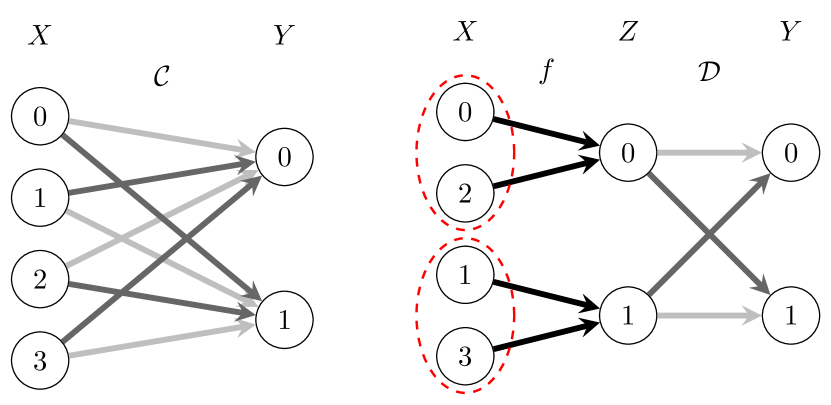
Figure 3: Factorizing the Redundant Binary Symmetric Channel: (Left) Channel from $X$ to $Y$. (Right) Intermediate variable $Z$ cleaves channel into two steps—first deterministic, then stochastic. Arrow shade indicates conditional probability: black: $1$, dark gray: $1-p$, and light gray: $p$. Dashed ellipses show input equivalence classes. (Note re-ordering of $X=1$ and $X=2$.)

To obtain the correct conditional distribution for $Y$, distinguishing $x=0$ from $x=2$ and also $x=1$ from $x=3$ are unnecessary. We eliminate this redundancy by mapping to intermediate variable $Z$ with the function $F:\mathcal{X}\rightarrow\mathcal{Z}$:

$$F(x)=\begin{cases}0\ ,\ x\in\{0,2\}\\ 1\ ,\ x\in\{1,3\}\end{cases}~{}.$$

The second factor (channel $\mathcal{C}^{{}^{\prime}}$) follows directly from this definition of $f$:

$$\mathbb{P}(Y=y|Z=z)=\bordermatrix{Z\backslash Y&0&1\cr 0&1-p&p\cr 1&p&1-p}~{},\qquad$$

Figure 3 shows this factorization for the RBSC channel.

It is fairly easy to see that $H_{\alpha}\left(Z\right)\leq H_{\alpha}\left(X\right)$ for any input random variable $X$ and all $\alpha\geq 0$. And so, this factorization represents a compression of the input information, without losing information necessary for obtaining the correct output distribution.

Now, consider the quantum map $\mathcal{E}:\mathcal{X}\to\mathcal{B}\left(\mathcal{H}\right)$, given by:

$$\mathcal{E}(x)=\begin{cases}\rho_{A}=\outerproduct{A}{A},&\text{for }x={0,2}\\ \rho_{B}=\outerproduct{B}{B},&\text{for }x={1,3}\end{cases}~{},$$

where:

$$\ket{A} \equiv\sqrt{1-p}\ket{0}+\sqrt{p}\ket{1}~{},$$

$$\ket{B} \equiv\sqrt{p}\ket{0}+\sqrt{1-p}\ket{1}~{},$$

with orthonormal basis $\{\ket{0},\ket{1}\}$. If we use the measurement $\mathcal{M}=\left\{\outerproduct{0}{0},\outerproduct{1}{1}\right\}$, we see that the channel is faithfully represented:

$$\mathbb{P}(Y=0|X=x\in\{0,2\}) =\braket{0}{\rho_{A}}{0}=1-p~{},$$

$$\mathbb{P}(Y=1|X=x\in\{0,2\}) =\braket{1}{\rho_{A}}{1}=p~{},$$

$$\mathbb{P}(Y=0|X=x\in\{1,3\}) =\braket{0}{\rho_{B}}{0}=p~{},$$

$$\mathbb{P}(Y=1|X=x\in\{1,3\}) =\braket{1}{\rho_{B}}{1}=1-p~{}.$$

Note that just as there were two classical intermediate states $\mathcal{Z}=\{0,1\}$ for the RBSC, there are two quantum signal states $\rho_{0}$ and $\rho_{1}$. For a given distribution over inputs $\mathbb{P}(X)$, we can also compare the entropy of the classical and quantum intermediate variables. The entropy of the quantum mixed state $\rho=\sum_{x\in\mathcal{X}}\mathbb{P}(x)\mathcal{E}(x)$ is given by the von Neumann entropy:

$$S(\rho)=-\tr(\rho\log{\rho})~{}.$$

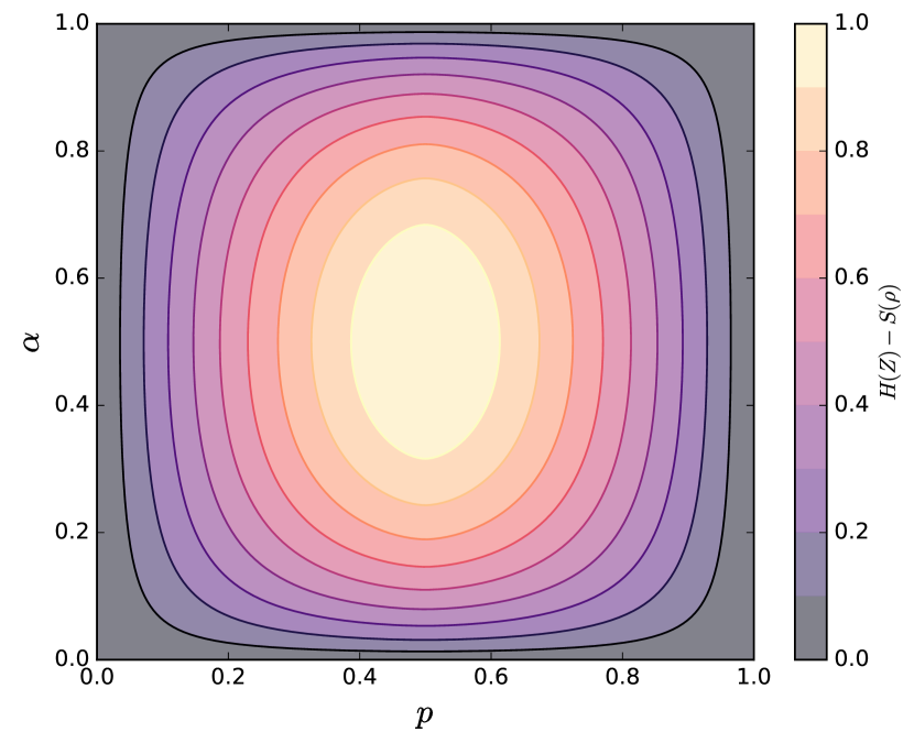
Figure 4: Factorization quantum advantage: $H({Z})-S(\rho)$ for quantum Redundant Binary Symmetric Channel with $\alpha=\mathbb{P}(Z=0)$; see Fig. 3. Maximum advantage occurs at $p=\alpha=\nicefrac{{1}}{{2}}$ and minima when $p=0$ or $\alpha=0$.

Importantly, this entropy is less than the classical entropy:

$$S(\rho)\leq H({Z})\leq H({X})~{},$$

for any input distribution $\mathbb{P}(X)$ [36, 37]. Figure 4 shows the quantum advantage $H(Z)-S(\rho)$ as a function of input distribution $\mathbb{P}(X\in\{0,2\})=\alpha$ and channel parameter $p$. The quantum factorization of the channel is, in this sense, more efficient than the reduced classical channel.

Consider a second example. Let $\mathcal{X}=\mathcal{Y}=\left\{\mathrm{A},\mathrm{B},\mathrm{C}\right\}$ and consider the channel $\mathcal{C}$, depicted in Fig. 5, given by the probabilities:

$$\mathbb{P}(Y=y|X=x)=\bordermatrix{X\backslash Y&\mathrm{A}&\mathrm{B}&\mathrm{C}\cr\mathrm{A}&2/3&1/6&1/6\cr\mathrm{B}&1/6&2/3&1/6\cr\mathrm{C}&1/6&1/6&2/3}~{}.$$

This channel is adapted from a stochastic process in Ref. [21], and we call it the 3-MBW channel after that process. Note that the channel is, effectively, its own causal factorization, as each $x\in X$ has a unique conditional distribution $\mathbb{P}\left(y\middle|x\right)$. Thus, the channel is already its strongly advantageous factorization. With uniform input $\mathbb{P}(x)=1/3$, we have $H_{\alpha}\left(X\right)=\log_{2}3$ for all $\alpha$.

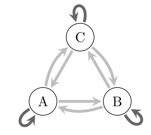
Figure 5: A channel that maps the set $\left\{\mathrm{A},\mathrm{B},\mathrm{C}\right\}$ to itself. Dark arrows represent probability $p=2/3$ of transition and light arrows $p=1/6$, so that all the outgoing edges of a node sum to $1$.

Two quantum models of this channel may be constructed. The first, which we call $\mathcal{Q}_{1}$, has a Hilbert space $\mathcal{H}_{1}$ spanned by the orthogonal basis $\left\{\ket{\mathrm{A}},\ket{\mathrm{B}},\ket{\mathrm{C}}\right\}$ with ensemble and POVM given by:

$$\mathcal{E}(x) =\outerproduct{\phi_{x}}{\phi_{x}}~{},$$

$$\ket{\phi_{x}} =\sum_{y\in\mathcal{Y}}\sqrt{\mathbb{P}\left(y\middle|x\right)}\ket{y}~{},~{}\text{and}$$

$$M_{y} =\outerproduct{y}{y}~{}.$$

Note that this induces the causal factorization. For the uniform input $\mathbb{P}(x)=1/3$, we get an entropy cost of $S(\rho)\approx 0.69$ qubits and a dimension cost of $S_{0}(\rho)=\log_{2}3$ qubits. Thus, we see the model improves on the classical case in entropy, but not in dimension. This type of model is inspired by the $q$-machine for processes [16] and generalizes easily to other channels.

The second model, which we call $\mathcal{Q}_{0}$, has a Hilbert space $\mathcal{H}_{0}$ spanned by the orthogonal basis $\left\{\ket{0},\ket{1}\right\}$ with ensemble and POVM given by:

$$\rho_{x} =\outerproduct{\psi_{x}}{\psi_{x}}~{},$$

$$\ket{\psi_{x}} =\begin{cases}\ket{0}&x=\mathrm{A}\\ \frac{1}{2}\ket{0}+\frac{\sqrt{3}}{2}\ket{1}&x=\mathrm{B}\\ \frac{1}{2}\ket{0}-\frac{\sqrt{3}}{2}\ket{1}&x=\mathrm{C}\end{cases}~{},~{}\text{and}$$

$$M_{y} =\frac{2}{3}\outerproduct{\psi_{y}}{\psi_{y}}~{}.$$

This, too, induces the causal factorization. For the uniform input, we get an entropy and dimension cost of $S(\rho)=S_{0}(\rho)=1$ qubits. In both of these quantifications, this model improves upon the classical case.

The other feature worth noting is that $\mathcal{Q}_{0}$ is advantageous over $\mathcal{Q}_{1}$ in the dimension cost $S_{0}$, but the opposite is true for the entropy cost $S_{1}$. (Indeed, this motivated the subscripts.) Reference [21] demonstrated that, for the Markov process version of this channel, the model $\mathcal{Q}_{0}$ was actually only two-dimensional model of the process. This result trivially carries over to the channel itself, which means $\mathcal{Q}_{0}$ is the model that uniquely minimizes $S_{0}$. However, it clearly does not minimize $S_{1}$. This demonstrates that, for at least this channel, no “strongly minimal” pure-state quantum model exists. This contrasts starkly to the causal factorization, which is strongly minimal among classical factorizations.

III Quantum Model Advantage

These examples hint at rather more general results on quantum advantage.

III.1 Single-shot: Constraints on minimal models

Our first pair of results is motivated by the questions: What models are optimal? And, how do they compare, generally, to the causal factorization for classical models?

We begin with the observation, stated earlier, that each quantum model $Q$ of a channel $\mathcal{C}$ induces a classical factorization $F_{Q}$. Recall that each induced factorization must be a refinement of the causal factorization $F_{\mathcal{C}}$.

Classically, a refinement to the causal factorization can be merged, where we combine causally equivalent inputs until the causal factorization is achieved, minimizing the Rényi entropies. Can we do the same for quantum models? There is, in fact, a process of state-merging that allows for the algorithmic reduction of any Rényi entropy individually.

The goal of state-merging is to combine the partitions of causally equivalent states. In this case, state merging on a quantum model means modifying an ensemble $\mathcal{E}(x)$, where $\mathcal{E}({x_{1}})\neq\mathcal{E}({x_{2}})$ for some $x_{1},x_{2}\in\mathcal{X}$ with $x_{1}\sim_{C}x_{2}$, into a new $\mathcal{E}^{\prime}(x)$ so that $\mathcal{E}^{\prime}({x_{1}})=\mathcal{E}^{\prime}({x_{2}})$. This can be accomplished in at least two ways:

1. $\mathcal{E}^{\prime}({x_{1}})=\mathcal{E}({x_{2}})$ and $\mathcal{E}^{\prime}({x})=\mathcal{E}({x})$ for $x\neq x_{1}$ or

2. $\mathcal{E}^{\prime}({x_{2}})=\mathcal{E}({x_{1}})$ and $\mathcal{E}^{\prime}({x})=\mathcal{E}({x})$ for $x\neq x_{2}$.

Recalling that the average model state is written as:

$$\rho=\sum_{x}\mathbb{P}(x)\mathcal{E}(x)~{},$$

we construct two new average model states:

$$\rho^{(1\rightarrow 2)} =\sum_{x\neq x_{1}}\mathbb{P}(x)\mathcal{E}(x)+\mathbb{P}(x_{1})\mathcal{E}(x_{2})~{}\text{and}$$

$$\rho^{(2\rightarrow 1)} =\sum_{x\neq x_{2}}\mathbb{P}(x)\mathcal{E}(x)+\mathbb{P}(x_{2})\mathcal{E}(x_{1})~{}.$$

Each results from two distinct forms of state merging. It is important to determine if such a technique reduces memory costs. This leads to a lemma that underlies our first main result.

Lemma 1.

Let $f:\mathbb{R}\rightarrow\mathbb{R}$ be a concave function and let $S_{f}(\rho)=\mathrm{Tr}\left(f(\rho)\right)$. Then:

$$S_{f}(\rho)\geq\min\{S_{f}(\rho^{(1\rightarrow 2)}),S_{f}(\rho^{(2\rightarrow 1)})\}~{}.$$ (3)

Proof.

Let $f:\mathbb{R}\rightarrow\mathbb{R}$ be a concave function and let $S_{f}(\rho)=\mathrm{Tr}\left(f(\rho)\right)$. Define:

$$\alpha =\mathbb{P}(x_{1})/(\mathbb{P}(x_{1})+\mathbb{P}(x_{2}))$$

$$1-\alpha =\mathbb{P}(x_{2})/(\mathbb{P}(x_{1})+\mathbb{P}(x_{2}))~{}.$$

One can check that:

$$\rho=\alpha\rho^{(1\rightarrow 2)}+(1-\alpha)\rho^{(2\rightarrow 1)}~{}.$$

By $f$’s concavity:

$$S_{f}(\rho) \geq\alpha S_{f}(\rho^{(1\rightarrow 2)})+(1-\alpha)S_{f}(\rho^{(2\rightarrow 1)})$$

$$\geq\min\{S_{f}(\rho^{(1\rightarrow 2)}),S_{f}(\rho^{(2\rightarrow 1)})\}~{}.$$ (4)

So, either $\rho^{(1\rightarrow 2)}$ or $\rho^{(2\rightarrow 1)}$ must be smaller according to $f$.

From this useful bound follows one of our primary results:

Result 1 (Causal Model Optimality).

A quantum model of a channel $\mathcal{C}$ minimizes $S_{f}\left(\rho\right)$, where $\rho$ is the average of the models’ ensemble and $f$ is any concave function, only if it induces the causal factorization of $\mathcal{C}$.

To see this, suppose otherwise: There exists a quantum model $\mathcal{Q}$ that does not induce the causal factorization, but that is $f$-minimal. By Eq. (3), though, we can perform a state-merging that yields a model $\mathcal{Q}^{\prime}$ with $S_{f}(\rho^{\prime})\leq S_{f}(\rho)$. This is a contradiction.

Of course, this result applies to the Rényi entropies $S_{\alpha}\left(\rho\right)$ as well: $S_{\alpha}\left(\rho\right)=S_{f}(\rho)/(1-\alpha)$, where $f(x)=x^{\alpha}$.

There are some caveats to this result. The first is that a minimum does not necessarily exist. The space of all possible models contains models of arbitrarily high Hilbert space dimension, and so it is not compact. This is still true even if we restrict to the space of models that induce the causal factorization: There is no restriction on the dimension of the states $\mathcal{E}(x)$.

However, if we restrict to pure-state models that induce the causal factorization, then the states $\mathcal{E}(x)$ can span a space of dimension no larger than $\dim\mathcal{H}=\left|\mathcal{Z}_{\mathcal{C}}\right|$. This makes the model-space compact and ensures the existence of a minimal model for each $S_{\alpha}$.

Now, in the classical case, the causal factorization was unique and strongly minimal, in that it minimized all $H_{\alpha}$. Our result shows that only quantum models that induce the causal factorization can be minimal. However, it does not prove that strongly minimal models exist. As we saw in the example of the 3-MBW channel, there may be models that are only weakly minimal, in that they only minimize some Rényi entropies and not others.

Our second main result focuses on comparing pure-state quantum models with the classical causal factorization itself. Pure-state quantum models, recall, are a quantum analogue to the factorization. Furthermore, as we just saw, pure-state quantum models that minimize any Rényi entropy must induce the causal factorization. Thus, to determine if and when they improve upon their classical counterpart, it makes sense to compare pure-state models that induce the causal factorization with the causal factorization itself.

Let $\mathcal{Q}$ be a pure-state quantum model that induces the causal factorization. Then its average model state is:

$$\rho=\sum_{z}\mathbb{P}(z)\ket{\psi_{z}}\bra{\psi_{z}}~{},$$

where the sum is over causal states $z\in\mathcal{Z}_{\mathcal{C}}$ and the states $\ket{\psi_{z}}$ correspond to the states of the quantum model: $\mathcal{E}(x)=\outerproduct{\psi_{z}}{\psi_{z}}$, if $z=f_{\mathcal{C}}(x)$.

We can also consider the orthogonal decomposition:

$$\rho=\sum_{i}\lambda_{i}\ket{i}\bra{i}~{}.$$

The vector of coefficients $\lambda_{i}$ and the probability distribution $\mathbb{P}(z)$ are related by a unitary matrix $U_{iz}$ such that [37]:

$$\mathbb{P}(z)=\sum_{i}\left|U_{iz}\right|^{2}\lambda_{i}~{}.$$

$U_{iz}$ is the identity matrix if and only if the states $\left\{\ket{\psi_{z}}\right\}$ are orthogonal. This establishes a majorization relationship between the two vectors, written $\lambda_{i}\succsim\mathbb{P}(z)$ [38]. The importance of this result here is that, for all concave $\alpha\geq 0$, we have $S_{\alpha}(\rho)\leq H_{\alpha}\left(Z_{\mathcal{C}}\right)$; with equality for $\alpha>0$ if and only if the states $\left\{\ket{\psi_{z}}\right\}$ are orthogonal.

This gives our second main result:

Result 2 (Strong/strict advantage of quantum models).

Given any input distribution $\mathbb{P}(x)$, a pure-state quantum model of a channel $\mathcal{C}$ that induces the causal factorization $F_{\mathcal{C}}$ satisfies $S_{\alpha}(\rho)\leq H_{\alpha}\left(Z_{\mathcal{C}}\right)$, where $\rho:=\sum_{x}\mathbb{P}(x)\mathcal{E}(x)$ is the average state. For $\alpha\geq 0$, the above bound is strict whenever the ensemble $\mathcal{E}(x)$ is nonorthogonal.

This result generalizes a similar result from Ref. [21] to channels. In fact, it strengthens it. Rather than $\mathbb{P}(z)$ being determined by a process’ unique stationary state distribution, here it can be determined by any input distribution $\mathbb{P}(x)$, and the quantum model state is still strongly advantageous.

III.2 Asymptotics: A lower bound

The previous section focused on pure states. Now, we return to mixed states to study the general asymptotic case.

Earlier we defined the $(n,M,\epsilon)$-quantum model. We introduce here a single-letter optimization that lower-bounds the rate $\frac{1}{n}\log M$ at which a channel can be quantally modeled, based on the classical Wyner common information. Unlike the classical case, we do not claim this bound is tight.

To set it up, consider a $d$-dimensional model $\left(\mathcal{H},\mathcal{E},\mathcal{M}\right)$ of the variables $XY$, with $\rho=\sum_{x}\mathbb{P}(x)\mathcal{E}(x)$. We define the Holevo information:

$$I_{\chi}\left(X:\rho\right)=S(\rho)-\sum_{x}\mathbb{P}(x)S\left(\mathcal{E}(x)\right)~{}.$$

For each state in the ensemble, we do an orthogonal decomposition:

$$\mathcal{E}(x)=\sum_{i=1}^{d}\lambda_{i|x}\outerproduct{i,x}{i,x}~{},$$

and define the conditional measurement information:

$$I_{\mu} \left(Y:\rho\middle|X\right)$$

$$=\sum_{x\in\mathcal{X}}\sum_{i=1}^{d}\mathbb{P}\left(x,i,y\right)\log\left(\frac{\mathbb{P}\left(i,y\middle|x\right)}{\mathbb{P}\left(y\middle|x\right)\lambda_{i|x}}\right)$$

where:

$$\mathbb{P}\left({x,i,y}\right)=\mathbb{P}(x)\lambda_{i|x}\braket{i,x}{M_{y}}{i,x}~{}.$$

(Note that $\mathbb{P}({x,y})=\sum_{i}\mathbb{P}\left({x,i,y}\right)$.) With these two, we define:

$$I\left(XY:\rho\right)=I_{\chi}\left(X:\rho\right)+I_{\mu}\left(Y:\rho\middle|X\right)~{}.$$

Another way to approach this quantity is to define:

$$\rho_{xy}=\sum_{i=1}^{d}\frac{\lambda_{i|x}\braket{i,x}{M_{y}}{i,x}}{\mathbb{P}\left(y\middle|x\right)}\ket{i,x}\bra{i,x}$$

as a state representing our knowledge, after the measurement, about what $i$ was before measurement. (This is not the final state after measurement, as the measurement itself induces further modification.) We then have:

$$I\left(XY:\rho\right)=S(\rho)-\sum_{x,y}\mathbb{P}\left(x,y\right)S\left(\rho_{xy}\right)~{}.$$

This is equivalent to our earlier definition, but expresses the quantity as a kind of Holevo quantity.

We define an analogue to the Wyner common information as:

$$C_{q,l}\left(X\middle>Y\right)=\inf_{X-\rho-Y}I\left(XY:\rho\right)~{}.$$

where $X-\rho-Y$ indicates that we are varying over all models of $XY$. The notation $\left.X\right>Y$ indicates that this is not a symmetric quantity between $X$ and $Y$.

Notice that we define this quantity as an infimum and not a minimum, as Wyner did. This is because Wyner’s proof [30] demonstrated that the infimum could be attained on a compact subset of the model space. This result relies on being able to decompose $I\left(XY:W\right)$ as $H\left(XY\right)-H\left(XY\middle|W\right)$. The minimization of $I\left(XY:W\right)$ becomes the maximization of $H\left(XY\middle|W\right)$. And this can be written as a linear function of $\mathbb{P}(w)$:

$$H\left(XY\middle|W\right)=-\sum_{w}\mathbb{P}(w)\sum_{x,y}\mathbb{P}\left(x,y\middle|w\right)\log\mathbb{P}\left(x,y\middle|w\right)~{},$$

if we hold $\mathbb{P}\left(x,y\middle|w\right)$ fixed.

It is the linearity of the optimization function, in the classical case, that allows the assumption of a compact minimization. However, our quantum generalization $I\left(XY:\rho\right)$ cannot be expressed in a way that allows the optimization to be linearized. This is why we cannot assume the existence of a minimum.

Our third main result can now be stated as follows.

Theorem 1.

Let $\delta>0$. Then there exists a fixed $\Delta>0$ such that, for all quantum $(n,M,\epsilon)$-models, $\frac{1}{n}\log M\leq C_{q,l}\left(X:Y\right)-\delta$ implies $\epsilon>\Delta$.

In other words, if the model’s cost rate is bounded below by $C_{q,l}$, then its error is bounded away from zero. To achieve arbitrary accuracy, it must have a rate of at least $C_{q,l}$.

Proof.

The argument follows the same logic as Wyner’s [30] and proceeds by contradiction. Suppose with $\delta$ fixed that, for any $\Delta>0$, we can find a $(n,M,\epsilon)$-model with $\frac{1}{n}\log M\leq C_{q,l}\left(X:Y\right)-\delta$ and $\epsilon<\Delta$. For such a model:

$$\frac{1}{n}\log M \geq\frac{1}{n}I\left(X^{n}\widehat{Y}^{n}:\rho\right)$$

$$\geq\frac{1}{n}H\left(X^{n}\widehat{Y}^{n}\right)-\frac{1}{n}H\left(X^{n}\widehat{Y}^{n}\middle|\rho\right)~{},$$

where:

$$H\left(X^{n}\widehat{Y}^{n}\middle|\rho\right) =H_{\chi}\left(X^{n}\middle|\rho\right)+H_{\mu}\left(Y^{n}\middle|\rho,X^{n}\right)~{},$$

$$H_{\chi}\left(X^{n}\middle|\rho\right) =H(X^{n})-I_{\chi}\left(X^{n}:\rho\right)~{},~{}\text{and}$$

$$H_{\mu}\left(\widehat{Y}^{n}\middle|\rho,X\right) =H\left(\widehat{Y}^{n}\right)-I_{\mu}\left(Y^{n}:\rho\middle|X^{n}\right)~{}.$$

We see that $H_{\mu}\left(\widehat{Y}^{n}\middle|\rho,X\right)$ is explicitly a conditional entropy by definition and so is subadditive. The subadditivity of $H_{\chi}\left(X^{n}\middle|\rho\right)$ is follows from the strong subadditivity of von Neumann entropy. Subadditivity implies that:

$$H\left(X^{n}\widehat{Y}^{n}\middle|\rho\right)\leq\sum_{k}H\left(X_{k}\hat{Y}_{k}\middle|\rho\right)~{}.$$

We then have:

$$\frac{1}{n}\log M \geq\frac{1}{n}H\left(X^{n}\widehat{Y}^{n}\right)-\frac{1}{n}\sum_{k}H\left(X_{k}\widehat{Y}_{k}\middle|\rho\right)~{}.$$

By assumption, we can drive $\Delta$ low enough that $H\left(X^{n}\widehat{Y}^{n}\right)\geq H(X^{n}Y^{n})-O\left(\Delta\right)$ where $O\left(\Delta\right)$ is the standard big-$O$ notation. Since $H\left(X^{n}Y^{n}\right)$ is separable, we can write $H\left(X^{n}\widehat{Y}^{n}\right)=\sum_{k}H\left(X_{k}\widehat{Y}_{k}\right)-O\left(\Delta\right)$ for some $\eta>0$. Thus:

$$\frac{1}{n}\log M \geq\frac{1}{n}\sum_{k}I\left(X_{k}\widehat{Y}_{k}:\rho\right)-O\left(\Delta\right)~{}.$$

This is a sum over a collection of single-letter models of channels that are at least $\Delta$-close to $XY$. Each such model is then $\Delta$-close to another model $\rho_{k}$ that perfectly generates $XY$. In each case we have $I\left(X_{k}\widehat{Y}_{k}:\rho\right)\geq I\left(XY:\rho_{k}\right)-O\left(\Delta\right)$. And, for each $k$ we have $I\left(XY:\rho_{k}\right)\geq C_{q,l}\left(X\middle>Y\right)$. Then:

$$\frac{1}{n}\log M \geq\frac{1}{n}\sum_{k}C_{q,l}\left(X\middle>Y\right)-O\left(\Delta\right)$$

$$=C_{q,l}\left(X\middle>Y\right)-\frac{1}{n}O\left(\Delta/n\right)~{}.$$

Now, take $\Delta$ small enough so that the error term is less than $n\delta$. We get:

$$\frac{1}{n}\log M \geq C_{q,l}\left(X\middle>Y\right)-\delta~{}.$$

However, this contradicts the assumption that $\frac{1}{n}\log M\leq C_{q,l}\left(X\middle>Y\right)-\delta$, completing the proof.

Thus, $C_{q,l}\left(X\middle>Y\right)$ offers a lower-bound on the rate at which one can model the channel $\mathcal{C}$. We now discuss the ways in which this lower-bound is lacking.

First, as we mentioned before, there is no guarantee that this bound can be easily computed via an optimization over a compact set. This arises from the optimization’s nonlinearity.

Second, it lacks a direct counterpart—that is, a theorem showing that $C_{q,l}\left(X\middle>Y\right)$ is achievable and not just a lower bound. Again, this stems from a fundamental difference between the setting of Wyner’s classical proof and the quantum models we are considering. Wyner’s achievability proof turns on showing that, given a single-shot model of a channel $\mathcal{C}$, one can take asymptotically many copies of the single-shot model and use random coding to trim off excess information.

For a quantum model, though, random coding means the random selection of subspaces. If the states $\rho_{x}$ of the ensemble commute, we may choose subspaces that commute with them all. Otherwise, coherence effects destroy the random coding approximation. In other words, there is a trade-off between minimizing the size of the single-shot model through the use of quantum coherence and, if coherence is present, the inability to further reduce the rate using asymptotic random coding. Finding an achievable lower bound on quantum models requires balancing these two tensions.

Finally, we note simply that $C_{q,l}\left(X\middle>Y\right)$ is not symmetric. While this may not seem necessary—after all, the channel simulation question is not one that is manifestly symmetric—we show in the following section that the quantum simulation of channels is equivalent to another question, involving entanglement, that is manifestly symmetric. We propose that this alternative formulation offers a more productive avenue of investigation.

III.3 Equivalence to common entanglement

Suppose we have a channel $\mathcal{C}:\mathcal{X}\rightarrow\mathcal{Y}$, a quantum model $\mathcal{Q}=\left(\mathcal{H},\mathcal{E},\mathcal{D}\right)$, and an input $X\sim\mathbb{P}(x)$. We will show how to reformulate these elements into a symmetric picture, where the joint random variable $XY$ is generated by taking local measurements on a bipartite entangled state $\ket{\Psi_{AB}}$. Just as the generation of a joint random variable from a classical shared variable with local operations is called common information, the generation of a joint random variable from shared entanglement is here called common entanglement.

For a mixed state $\rho$ on a space $\mathcal{H}_{B}$ with dimension $d$, we can write its orthogonal decomposition as:

$$\rho=\sum_{i=1}^{d}\lambda_{i}\ket{i}_{B}\ket{i}_{B}~{}.$$

We assume without loss of generality that $\mathcal{H}_{B}$ is entirely spanned by $\rho$’s support; that is, $\lambda_{i}>0$ for all $i=1,\dots,d$. We define $\rho$’s purification as a state that exists on the space $\mathcal{H}_{A}\otimes\mathcal{H}_{B}$, where $\mathcal{H}_{A}$ is a copy of $\mathcal{H}_{B}$ with dimension $d$ as well. $\rho$’s purification is:

$$\ket{\psi}_{AB}=\sum_{i=1}^{d}\sqrt{\lambda_{i}}\ket{i}_{A}\otimes\ket{i}_{B}~{},$$

where the basis $\{\ket{i}_{A}\}$ is unitarily equivalent to the original $\{\ket{i}_{B}\}$. It is a purification in the sense that $\mathrm{Tr}_{B}\left(\ket{\psi}_{AB}\right)=\rho$. That is, one can imagine the mixed state only exists due to ignorance of a larger system. Up to unitary transformations on $\mathcal{H}_{A}$, this purification is unique.

Ensembles $\mathcal{E}:\mathcal{X}\rightarrow\mathcal{B}_{+}\left(\mathcal{H}\right)$ may also be purified. Our scheme here resembles that in Ref. [39] except that we allow the ensemble states $\mathcal{E}\left(x\right)$ to be mixed. Given an input $\mathbb{P}\left(x\right)$, we write:

$$\rho =\sum_{x\in\mathcal{X}}\mathcal{E}(x)$$

$$=\sum_{x\in\mathcal{X}}\mathbb{P}(x)\rho_{x}$$

as the ensemble decomposition of $\rho$ on $\mathcal{H}_{B}$. Let $\ket{\psi}_{AB}$ be a purification of $\rho$ and $\ket{\psi_{x}}_{AB}$ be a purification of the unnormalized state $\mathbb{P}(x)\mathcal{E}(x)$ (both onto $\mathcal{H}_{A}\otimes\mathcal{H}_{B}$).

Letting $\left\{\ket{i,x}\right\}$ be the diagonalizing basis of $\mathbb{P}(x)\mathcal{E}(x)$ and $\lambda_{i|x}$ be its spectra, we can write:

$$\ket{\psi_{x}}_{AB} =\sum_{i=1}^{d}\sqrt{\lambda_{i|x}}\ket{i,x}_{A}\otimes\ket{i,x}_{B}$$

$$=\sum_{j=1}^{d}\sum_{i=1}^{d}\sqrt{\lambda_{i|x}}\ket{i,x}_{A}\otimes\left(\braket{j}{i,x}\ket{j}_{B}\right)$$

$$=\sum_{j=1}^{d}\sqrt{\lambda_{j}}\left(\sum_{i=1}^{d}\sqrt{\frac{\lambda_{i|x}}{\lambda_{i|x}}}\braket{j}{i,x}\ket{i,x}_{A}\right)\otimes\ket{j}_{B}$$

$$=\sum_{\omega\in\Omega}\sqrt{\lambda_{j}}\ket{\Phi_{j,x}}_{A}\otimes\ket{j}_{B}~{},$$

where:

$$\ket{\Phi_{j,x}}_{A}=\sum_{i=1}^{d}\sqrt{\frac{\lambda_{i|x}}{\lambda_{j}}}\braket{j}{i,x}\ket{i,x}_{A}$$

For each $x\in\mathcal{X}$, there is a unique operator $K_{x}$ on $\mathcal{H}_{A}$ such that:

$$K_{x}\ket{j}_{A}=\ket{\Phi_{j,x}}_{A}~{}.$$

Furthermore:

$$\braket{j}{\sum_{x}K^{\dagger}_{x}K_{x}}{j^{\prime}} =\sum_{x\in\mathcal{X}}\braket{\Phi_{j,x}}{\Phi_{j^{\prime},x}}$$

$$=\sum_{x\in\mathcal{X}}\sum_{i=1}^{d}\frac{\lambda_{i|x}}{\sqrt{\lambda_{j}\lambda_{j^{\prime}}}}\braket{j}{i,x}\braket{i,x}{j^{\prime}}$$

$$=\frac{1}{\sqrt{\lambda_{j}\lambda_{j^{\prime}}}}\braket{j}{\rho}{j^{\prime}}=\delta_{jj^{\prime}}~{}.$$

This shows that the $\left\{K_{x}\right\}$ are the Kraus operators of a complete POVM $\mathcal{M}=\left\{M_{x}\right\}$ with $M_{x}=K_{x}^{\dagger}K_{x}$.

To summarize, an ensemble $\mathcal{E}(x)$ has a unique purification $\left(\ket{\psi}_{AB},\mathcal{M}_{A}\right)$ satisfying:

$$\mathrm{Tr}\left(\outerproduct{\psi}{\psi}_{AB}\right) =\rho_{B}$$

$$\mathrm{Tr}\left(M_{x}\outerproduct{\psi}{\psi}_{AB}\right) =\mathbb{P}\left(x\right)\mathcal{E}\left(x\right)~{},$$

where $\rho_{B}=\sum_{x}\mathbb{P}(x)\mathcal{E}(x)$. This purification is unique up to transformations of the form $K_{x}\mapsto UK_{x}V^{\dagger}_{x}$ for unitary matrices $U$ and $\left\{V_{x}\right\}$ on $\mathcal{H}_{A}$. (These arise from the unitary ambiguity of each individual purification of $\rho$ and $\mathcal{E}(x)$.)

Correspondingly, the common entanglement representation of a quantum model $\mathcal{Q}=\{\mathcal{H}_{B},\mathcal{E},\mathcal{M}\}$ is the triplet $\Phi=\left(\ket{\Phi}_{AB},\mathcal{M}_{A},\mathcal{M}_{B}\right)$, where $\left(\ket{\Phi}_{AB},\mathcal{M}_{A}\right)$ is the purification of the ensemble $\mathcal{E}$ and $\mathcal{M}_{B}=\mathcal{M}$.

In this representation the distribution $\mathbb{P}\left(x,y\right)$ is seen as being generated by the local POVM $\mathcal{M}_{A}\otimes\mathcal{M}_{B}=\left\{M_{x}\otimes N_{y}\right\}$ from a shared entangled pair. In the language of entanglement theory the representation is equivalent to simulating the channel via a quantum ensemble. See Fig. 6.

Figure 6: Two equivalent pictures: (Top) Directional picture modeling a channel $\mathcal{C}:\mathcal{X}\rightsquigarrow\mathcal{Y}$ with an intermediate quantum system $\rho$. (Bottom) Symmetric picture generating a joint random variable $XY$ from an entangled state $\ket{\Phi}_{AB}$.

For every quantum model $\mathcal{Q}=\{\mathcal{H}_{B},\mathcal{E},\mathcal{M}\}$ of the channel $\mathcal{C}:\mathcal{X}\rightsquigarrow\mathcal{Y}$ and input random variable $X\sim\mathbb{P}\left(x\right)$, the joint random variable $XY$ has a common entanglement generator $\Phi=\left(\ket{\Phi}_{AB},\mathcal{M}_{A},\mathcal{M}_{B}\right)$. This alternative perspective on the reverse Holevo problem will prove fruitful for future extensions of our results.

IV Concluding remarks

We inverted the question originally posed by Holevo. Rather than using classical resources to quantify the behavior of quantum channels, we analyzed how well quantum resources may simulate the workings of a classical channel.

This question makes sense in the context of wider considerations. We do not claim that it is practically efficient to replace classical channels with quantum ones. Attempts to construct and use quantum channels, such as in quantum teleportation, often require classical communication to work. However, this is a consequence of the difficulties in transmitting quantum information over distances. When we discuss channels as a microcosm of the inner workings of a stochastic process, in contrast, we are invoking information that is retained over time. This information is memory. When we measure the Rényi entropies of the average quantum state of a model, we are subjecting it to various memory metrics.

Thus, our results here are best interpreted as a study not in spatial communication, but in the memory required to simulate a temporal channel. In this setting, we showed that:

1. In the single-shot regime, those quantum models minimizing various memory metrics are those that induce the causal state.

2. Conversely, pure-state models that induce the causal state improve upon the best classical factorization across all memory metrics, and

3. In the asymptotic regime, for arbitrary accuracy to be achieved the quantum memory rate required for simulation is bounded below by the new quantum common information quantity for channels—$C_{q,l}\left(X\middle>Y\right)$—introduced here.

Many questions remain. For instance, under what conditions is $C_{q,l}\left(X\middle>Y\right)$ achievable? When it is not, can we derive a tighter lower bound? The common entanglement representation of the problem in Section III.3 should prove useful in furthering study of these questions.

It also remains to rigorously connect our results for channels back to the problem of simulating stochastic processes with quantum resources. The rates achievable for channels can be applied to the process channel $\mathbb{P}\left(x_{0:\infty}\middle|x_{-\infty:0}\right)$ from the past to the future. These would give lower bounds on the rates at which we can sequentially generate a process. Likely, they would not be tight. Thus, as results for simulating channels are derived, the additional constraints characterizing sequential generation must also be formulated.

References

- [1] D. A. Meyer. Quantum computing classical physics. Phil. Trans. Roy. Soc. London A, 360(1792):395–405 1364–503X, 2002.
- [2] M. H. Yung, D. Nagaj, J. D. Whitfield, and A. Aspuru-Guzik. Simulation of classical thermal states on a quantum computer: A transfer-matrix approach. Phys. Rev. A, 82(6):060302, 2010.
- [3] J. Yepez. Quantum lattice-gas model for computational fluid dynamics. Phys. Rev. E, 63(4):046702, 2001.
- [4] J. Yepez. Quantum computation of fluid dynamics. In Quantum Computing and Quantum Communications, pages 34–60. Springer, 1999.
- [5] S. Sinha and P. Russer. Quantum computing algorithm for electromagnetic field simulation. Quant. Info. Processing, 9(3):385–404
- [6] J. Yepez. Quantum lattice-gas model for the diffusion equation. Intl. J. Mod. Physics C, 12(09):1285–1303
- [7] G. P. Berman, A. A. Ezhov, D. I. Kamenev, and J. Yepez. Simulation of the diffusion equation on a type-ii quantum computer. Phys. Rev. A, 66(1):012310, 2002.
- [8] J. Yepez. Quantum lattice-gas model for the Burgers equation. J. Stat. Physics, 107(1-2):203–224
- [9] S. A. Harris and V. M. Kendon. Quantum-assisted biomolecular modelling. Phil. Trans. Roy. Soc. London A, 368(1924):3581–3592 1364–503X, 2010.
- [10] P. W. Shor. Polynomial-time algorithms for prime factorization and discrete logarithms on a quantum computer. SIAM Review, 41(2):303–332
- [11] L. K. Grover. A fast quantum mechanical algorithm for database search. In Proceedings of the Twenty-Eighth Annual ACM Symposium on Theory of Computing, pages 212–219
- [12] A. W. Harrow, A. Hassidim, and S. Lloyd. Quantum algorithm for linear systems of equations. Phys. Rev. Let., 103(15):150502, 2009.
- [13] J. P. Crutchfield and K. Young. Inferring statistical complexity. Phys. Rev. Let., 63:105–108, 1989.
- [14] C. R. Shalizi and J. P. Crutchfield. Computational mechanics: Pattern and prediction, structure and simplicity. J. Stat. Phys., 104:817–879, 2001.
- [15] J. P. Crutchfield. Between order and chaos. Nature Physics, 8:17–24, 2012.
- [16] M. Gu, K. Wiesner, E. Rieper, and V. Vedral. Quantum mechanics can reduce the complexity of classical models. Nature Comm., 3(762), 2012.
- [17] R. Tan, D. R. Terno, J. Thompson, V. Vedral, and M. Gu. Towards quantifying complexity with quantum mechanics. Eur. J. Phys. Plus, 129:191, 2014.
- [18] J. R. Mahoney, C. Aghamohammadi, and J. P. Crutchfield. Occam’s quantum strop: Synchronizing and compressing classical cryptic processes via a quantum channel. Scientific Reports, 6(20495), 2016.
- [19] P. M. Riechers, J. R. Mahoney, C. Aghamohammadi, and J. P. Crutchfield. A closed-form shave from Occam’s quantum razor: Exact results for quantum compression. Phys. Lett. A, 93:052317, 2016.
- [20] F. C. Binder, J. Thompson, and M. Gu. A practical, unitary simulator for non-Markovian complex processes. Phys. Rev. Lett., 120:240502, 2017.
- [21] S. Loomis and J. P. Crutchfield. Strong and weak optimizations in classical and quantum models of stochastic processes. J. Stat. Phys., 176(6):1317–1342, 2019.
- [22] Q. Liu, T. J. Elliot, F. C. Binder, C. D. Franco, and M. Gu. Optimal stochastic modelling with unitary quantum dynamics. arXiv:1810.09668.
- [23] C. Bennett, P. W. Shor, J. A. Smolin, and A. V. Thapliyal. Entanglement-assisted classical capacity of noisy quantum channels. Phys. Rev. Lett., 83:3081, 1999.
- [24] C. Bennett, P. W. Shor, J. A. Smolin, and A. V. Thapliyal. Entanglement-assisted capacity of a quantum channel and the reverse Shannon theorem. IEEE Trans. Inf. Theory, 48, 2002.
- [25] C. Bennett, I. Devetak, A. W. Harrow, P. W. Shor, and A. Winter. The quantum reverse Shannon theorem and resource tradeoffs for simulating quantum channels. IEEE Trans. Inf. Theory, 60, 2014.
- [26] A. S. Holevo. Bounds for the quantity of information transmitted by a quantum communication channel. Problems of Information Transmission, 9:177, 1973.
- [27] B. Schumacher and M. Westmoreland. Sending classical information via noisy quantum channels. Phys. Rev. A, 56:131, 97a.
- [28] A. S. Holevo. Coding theorems for quantum channels. Russian Math. Surveys, 53:1295–1331, 1996.
- [29] A. S. Holevo. The capacity of quantum channel with general signal states. IEEE Trans. Inf. Theory, 44, 1998.
- [30] A. D. Wyner. The common information of two dependent random variables. IEEE Trans. Inf. Theory, 21, 1975.
- [31] G. R. Kumar, C. T. Li, and A. El Gamal. Exact common information. In 2014 IEEE ISIT, page 161. IEEE, 2014.
- [32] A. B. Boyd, D. Mandal, and J. P. Crutchfield. Thermodynamics of modularity: Structural costs beyond the Landauer bound. Phys. Rev. X, 8(3):031036, 2018.
- [33] R. A. Ahlswede and A. Winter. Strong converse for identification via quantum channels. IEEE Trans. Inf. Theory, 48:346, 2002. Addendum: IEEE Trans. Inf. Theory, vol. 49, no. 1, p. 346, 2003.
- [34] A. Winter. Secret, public and quantum correlation cost of triples of random variables. In 2005 IEEE ISIT. IEEE, 2005.
- [35] R. B. Ash. Information Theory. Dover, New York, 1990.
- [36] A. Wehrl. General properties of entropy. Rev. Mod. Physics, 50(2):221, 1978.
- [37] L. P. Hughston, R. Jozsa, and W. K. Wootters. A complete classification of quantum ensembles having a given density matrix. Phys. Lett. A, 183(1):14–18, 1993.
- [38] A. W. Marshall, I. Olkin, and B. C. Arnold. Inequalities: Theory of Majorization and Its Applications. Springer, New York, NY, 3 edition, 2011.
- [39] G. Ghirardi A. Bassi. A general scheme for ensemble purification. Phys. Lett. A, 309:24, 2003.