Non-integrable dynamics of matter-wave solitons in a density-dependent gauge theory

Abstract

We study interactions between bright matter-wave solitons which acquire chiral transport dynamics due to an optically-induced density-dependent gauge potential. Through numerical simulations, we find that the collision dynamics feature several non-integrable phenomena, from inelastic collisions including population transfer and radiation losses to short-lived bound states and soliton fission. An effective quasi-particle model for the interaction between the solitons is derived by means of a variational approximation, which demonstrates that the inelastic nature of the collision arises from a coupling of the gauge field to velocities of the solitons. In addition, we derive a set of interaction potentials which show that the influence of the gauge field appears as a short-range potential, that can give rise to both attractive and repulsive interactions.

I Introduction

One of the defining properties of solitons in systems such as the nonlinear Schrödinger (NLS) and Korteweg-de Vries equations is that they pass through and emerge from collisions with other solitons unperturbed, with the exception of a phase shift arising from the nonlinear interaction. tome ; solbook . All of the dynamical quantities of solitons, such as their velocities and masses, are conserved during the collision. In such systems, the elastic nature of these collisions is a consequence of the integrability of the model, which heavily restricts the allowed dynamics due to the existence of an infinite set of conservation laws.

In non-integrable systems, stable solitons may exist too, but their collisions are, generally, inelastic and can lead to trajectories which are chaotic tome ; solbook2 . In this case, the defining feature is the existence of short-lived bound states in which the number of collision events depends fractally on the initial conditions. Generally, this mechanism arises from the excitation of an internal mode of the solitons in non-integrable models, either with chaos5 ; chaos6 ; chaos7 ; chaos10 ; chaos11 or without radiation losses chaos8 ; chaos9 , or through the presence of a weak perturbation chaos1 ; chaos2 ; chaos4 . Solitons can merge or fracture into new products through fission and fusion processes fusfis1 ; fusfis2 ; fusfis3 , which has also been studied in the context of three-soliton and soliton-breather collisions boris3 . These effects highlight a strong contrast to soliton dynamics in integrable systems, which are not only interesting from a fundamental point of view, but offer insight into the description of realistic systems where the influence of perturbations can be consequential.

Ultracold atomic gases represent an attractive platform to study nonlinear physics due to their unprecedented experimental controllability. The ability to precisely engineer both the dimensionality and interactions in these systems has lead to the realization of isolated bright matter-wave solitons sol1 ; bsw2 , as well as solitons trains sol2 . The second generation of experiments addressed controlled collisions with potential barriers marchant_2013 ; marchant_2016 , as well as understanding both the role and origin of the relative phase for the stability of bright soliton states trapcoldcol1 ; nguyen_2017 ; everitt_2017 .

The underlying integrability of the focusing nonlinear Schrödinger equation leads to a hierarchy of analytical higher-order soliton solutions provided by the inverse scattering transform. This directly led to the development of a classical particle model trapcoldcol3 , describing the dynamics of the bright solitons, from which regions of chaotic behaviour have been eventually predicted for trapped bright solitons in non-integrable settings trapcoldcol4 ; martin_2008 .

Due to their inherent coherence, bright solitons represent a useful tool for investigating interferometry in the quantum realm. Recent experimental progress in this direction has seen the first realization of a ⁸⁵Rb matter-wave Interferometer, as well as theoretical proposals for precision measurement using the Sagnac effect helm_2015 and the creation of Bell states using quantum bright solitons gertjerenken_2013 , as well taking advantage of the interaction of solitons with nonlinear splitters HS .

The ability to simulate artificial gauge theories with ultracold gases offers a new opportunity to understand the interplay of effective magnetism in these systems with nonlinear effects dalibard_2011 ; Lightgauge . This has led to the realization of vortex states lin_2009 as well as spin-orbit coupling lin_2011 . Interest was recently focused on schemes for generating gauge potentials with an effective back-action between the matter and the gauge potential intgauge ; intgauge3 , which leads to a number of novel phenomena, including the violation of the Kohn’s theorem matt1 ; intgauge2s , and unconventional vortex dynamics giulio1 ; giulio2 . Very recently, the first experimental realization of a dynamical gauge theory in a trapped ion system was shown martinez_2016 .

In this paper, we study the nonlinear dynamics of two interacting one-dimensional chiral matter-wave solitons. We begin by reviewing how these solitons can be engineered in ultracold gases using optical techniques which induce an effective density-dependent gauge potential in the atomic cloud. The resulting equation of motion for the gas, which takes the form of a chiral nonlinear Schrödinger equation, is then solved numerically in Sec. III. Following this in Sec. IV, we develop a variational approach to further understand the soliton dynamics in this system, both in linear and asymptotic limits, before concluding in Sec. V.

II The theoretical model

We consider a Bose-Einstein condensate of $N$ two-level interacting atoms, in which two internal states of the atoms (labelled $\ket{1}$ and $\ket{2}$) are resonantly coupled by an external laser field. The Hamiltonian describing the interacting trapped gas as well as the light-matter interaction can be written as

$$\hat{H}=\bigg{(}\frac{\hat{\mathbf{p}}^{2}}{2m}+\frac{1}{2}m\omega_{\perp}^{2}\mathbf{r}_{\mathrm{\perp}}^{2}\bigg{)}\otimes\mathbb{I}+\hat{H}_{\mathrm{lm}}+\hat{\mathcal{V}}_{\mathrm{int}},$$ (1)

where

$$\hat{H}_{\mathrm{lm}}=\frac{\hbar\Omega}{2}\bigg{(}\begin{array}[]{cc}0&e^{-i\phi_{\ell}}\\ e^{i\phi_{\ell}}&0\end{array}\bigg{)}$$ (2)

describes the optical coupling of the two internal states of the atoms, with strength $\Omega$ and laser phase $\phi_{\ell}$. In order to obtain an equation of motion for the many-particle system, the state of the system is defined as a Hartree product $\ket{\Psi}=\otimes_{l=1}^{N}\ket{\chi_{l}^{(0)}}$, where $\ket{\chi_{l}^{(0)}}$ defines one of the single-particle eigenstates of Eq. (2). In this work we assume that the gas is harmonically trapped in the $\left(x,y\right)$ plane (described by the vectorial $\mathbf{r}_{\perp}$ coordinates in Eq. (2)), but free along the axial $z$ direction. The mean-field interactions appearing in Eq. (1) are defined by $\hat{\mathcal{V}}_{\mathrm{int}}=\text{diag}[g_{11}|\Phi_{1}|^{2}+g_{12}|\Phi_{2}|^{2},g_{22}|\Phi_{2}|^{2}+g_{12}|\Phi_{1}|^{2}]$, where $|\Phi_{i}|^{2}$ denotes the population of the state $i$.

Provided that the gas is sufficiently dilute, we can diagonalize the Hamiltonian by treating the mean-field interactions $g_{ii^{\prime}}|\Phi_{i}|^{2}$ as a small perturbation to the laser coupling $\hbar\Omega$. The eigenvectors of Eq. (1) can then be written in the dressed state basis $\{+,-\}$ as

$$|\chi_{\pm}\rangle=|\chi^{(0)}_{\pm}\rangle+\frac{g_{11}-g_{22}}{8\hbar\Omega}|\Phi_{\pm}|^{2}|\chi^{(0)}_{\mp}\rangle,$$ (3)

where $|\chi^{(0)}_{\pm}\rangle=\left(|1\rangle\pm e^{i\phi_{\ell}}|2\rangle\right)/\sqrt{2}$ denotes the unperturbed dressed states. The associated eigenvalues are given by $g|\Phi_{\pm}|^{2}\pm\hbar\Omega/2$, with the dressed scattering parameter $g=(g_{11}+g_{22}+2g_{12})/4$.

From the interacting dressed states, we can write the state vector of the system as $\ket{\xi}=\sum_{i=+,-}\Phi_{i}\left(\mathbf{r},t\right)|\chi_{i}\rangle$. Then, the effective Hamiltonian is written as

$$\hat{H}_{\pm}=\frac{1}{2m}(\mathbf{p}-\mathbf{A}_{\pm})^{2}+\frac{1}{2}m\omega_{\perp}^{2}\mathbf{r}_{\perp}^{2}+\frac{g}{2}|\Phi_{\pm}|^{2}.$$ (4)

Equation (4) introduces the geometric phase $\mathbf{A}_{\pm}=i\hbar\langle\chi_{\pm}|\nabla\chi_{\pm}\rangle$. Accompanying this is a scalar geometric phase, whose leading-order effect is inducing an energy offset, which may be dropped. Then, using the definition given by Eq. (3), to lowest-order the density-dependent geometric phase appears as $\mathbf{A}_{\pm}=\mathbf{A}^{(0)}+\mathbf{a}_{1}|\Phi_{\pm}(\mathbf{r})|^{2}$, with the single-particle vector potential, $\mathbf{A}^{(0)}=-\frac{\hbar}{2}\nabla\phi_{l}(\mathbf{r})$, while $\mathbf{a}_{1}=\nabla\phi_{l}(\mathbf{r})(g_{11}-g_{22})/8\Omega$ defines the strength of the density-dependent gauge potential. The equation of motion governing the evolution of the wave-function amplitude $\Phi_{+}\left(\mathbf{r},t\right)$ is found from minimization of the system’s energy functional, $\mathcal{E}=\langle\Psi|(i\hbar\partial_{t}-\hat{H}_{\pm})|\Psi\rangle$. After dropping $\pm$ subscripts, the resulting mean-field density-dependent Gross-Pitaevskii equation is obtained as

$$i\hbar\frac{\partial\Phi}{\partial t}=\left[\frac{1}{2m}\left(\mathbf{p}{-}\mathbf{A}\right)^{2}{+}\mathbf{a_{1}}\cdot\mathbf{j}{+}\frac{1}{2}m\omega_{\perp}^{2}\mathbf{r}_{\perp}^{2}{+}g|\Phi|^{2}\right]\Phi,$$ (5)

where

$$\mathbf{j}=\frac{1}{2m}\bigg{[}\Phi\left(\mathbf{p}+\mathbf{A}\right)\Phi^{\ast}-\Phi^{\ast}\left(\mathbf{p}-\mathbf{A}\right)\Phi\bigg{]}.$$ (6)

defines the current nonlinearity appearing in Eq. (5). The current-coupled nonlinear Schrödinger equation, captured by Eq. (5), describes a novel nonlinear gauge theory where there is an effective back-action between the matter-field and the gauge potential intgauge . This feedback ingredient of the system is somewhat similar to the local field effect, which affects a “soft” optical lattice trapping the condensate, that gives rise to various consequences, such as formation of bright solitons in the absence of contact interactions between atoms GDong .

II.1 One-dimensional reduction

We are interested in studying solitary-wave solutions in the frameworks of the dimensionally reduced form of Eqs. (5) and (6). To do this, we assume the system is in the ground state of the transverse trap, such that one can factorize the wave function as $\Phi(\mathbf{r},t)=\Psi_{\perp}(\mathbf{r}_{\perp})\Psi(x,t)$, where $\Psi_{\perp}(\mathbf{r}_{\perp})=(\sqrt{\pi}l_{\perp})^{-1}\exp(-\mathbf{r}_{\perp}^{2}/2l_{\perp}^{2})$ is the transverse ground-state wave function, and $l_{\perp}=\sqrt{\hbar/m\omega_{\perp}}$ is the transverse harmonic length scale. Equation (5) is then reduced to an effective one-dimensional form,

$$i\hbar\frac{\partial\Psi}{\partial t}=\left[\frac{1}{2m}\left(\hat{p}-a_{1}|\Psi|^{2}\right)^{2}+a_{1}j(x)+g_{\mathrm{1D}}|\Psi|^{2}\right]\Psi,$$ (7)

where both the scattering parameters $a_{1}=k(g_{11}-g_{22})/(16\pi l_{\perp}^{2}\Omega)$ and $g_{\mathrm{1D}}=g/(2\pi l_{\perp}^{2})$ have been scaled by the transverse area of the cloud, and the corresponding one-dimensional current nonlinearity is defined as

$$j(x)=\frac{1}{2m}\bigg{[}\Psi\left(\hat{p}{+}a_{1}|\Psi|^{2}\right)\Psi^{\ast}{-}\Psi^{\ast}\left(\hat{p}{-}a_{1}|\Psi|^{2}\right)\Psi\bigg{]}.$$ (8)

In writing Eq. (7), we have defined the laser phase as $\phi_{\ell}=kx$ and subsequently eliminated the zeroth-order vector potential through a momentum boost. We can further simplify Eq. (7) by introducing the nonlinear phase transformation

$$\Psi(x,t)=\psi(x,t)\text{ exp}\left(\frac{ia_{1}}{\hbar}\int_{-\infty}^{x}dx^{\prime}|\psi(x^{\prime},t)|^{2}\right),$$ (9)

which acts to decouple the vector potential from the canonical momentum appearing in the one-dimensional Gross-Pitaevskii equation. Substituting Eq. (9) into Eq. (7) and (8) leads to the simplified equation,

$$i\hbar\frac{\partial\psi}{\partial t}=\bigg{[}-\frac{\hbar^{2}}{2m}\partial_{x}^{2}-2a_{1}j^{\prime}(x)+g_{\mathrm{1D}}|\psi|^{2}\bigg{]}\psi,$$ (10)

where $j^{\prime}(x)=(\hbar/m)\text{Im}(\psi^{\ast}\partial_{x}\psi)$ is the gauge-transformed current operator. Equation (10) belongs to the class of derivative or ‘chiral’ NLS equations derivNLS ; chiral1 , which was originally studied, in particular, in the context of one-dimensional anyons anyon2 . The model features several key differences from the standard NLS equation in that it is generally non-integrable, does not obey the Galilean invariance, and possesses chiral soliton solutions anyon ; anyon2 ; chiral1 . These properties are expected to contribute to unconventional soliton dynamics in the one-dimensional case.

An experimental realization of the interacting gauge theory relies, basically, on two conditions, $viz$., an atomic species possessing long-lived excited states that the adiabatic motion of the atoms requires, as well as the spontaneous-emission rate that is negligible on the time scale of cold-atom experiments. A promising candidate that fulfils these conditions are alkali-earth atoms, which have been recently used to create a spin-orbit-coupled Fermi gas of ¹⁷³Yb atoms song_2016 , using a methodology similar to that outlined here. Very recently, an interaction-induced synthetic gauge potential was realised experimentally in a Bose-Einstein condensate loaded into a modulated two-dimensional lattice Clark_2018 .

II.2 Chiral solitons

Single-soliton solutions of Eq. (10) can be derived by first boosting into the moving frame via the transformation

$$\psi_{\mathrm{BS}}(x,t)=\varphi(x-vt)e^{i(mvx^{\prime}+mv^{2}t^{\prime}/2-\mu t^{\prime})/\hbar},$$ (11)

which consists of a Galilean transformation in which the stationary coordinates $(x,t)$ and moving coordinates $(x^{\prime},t^{\prime})$ are connected by the translations, $x^{\prime}\rightarrow x-vt$ and $t^{\prime}\rightarrow t$, with frame velocity $v$. The resulting differential equation for the real-valued wave function $\varphi(x^{\prime})$ becomes

$$\mu\varphi=-\frac{\hbar^{2}}{2m}\frac{d^{2}}{d{x^{\prime}}^{2}}\varphi+\left(g_{\mathrm{1D}}-2a_{1}v\right)\varphi^{3},$$ (12)

in which the current is contained as $j(x)=v\varphi^{2}$. Integrating Eq. (12), and requiring that the wave function converges to $\varphi(\pm\infty)=0$ for $g_{\mathrm{1D}}^{\prime}=g_{\mathrm{1D}}-2a_{1}v<0$, one finds the single bright-soliton solution,

$$\psi_{\mathrm{BS}}={\frac{1}{\sqrt{2b}}}\operatorname{sech}\left(\left(x-vt\right)/b\right)e^{i\left(mvx-mv^{2}t/2-\mu t\right)/\hbar},$$ (13)

in which we have transformed back into the stationary frame. The chemical potential appearing in Eq. (12) is $\mu=-mg_{\mathrm{1D}}^{2\prime}N^{2}/8\hbar^{2}$, with the amplitude factor $1/\sqrt{2b}$ provided normalization $N=1$. In contrast to the Gross-Pitaevskii theory used to model non-chiral bright solitons PandS , the lack of the Galilean invariance of Eq. (10) results in a change of the soliton width, $b=-2\hbar^{2}/mg_{\mathrm{1D}}^{\prime}$, depending on the direction of the soliton’s motion. These solitons are therefore chiral, in the sense that the mean-field interactions, and hence the soliton’s size depend on the direction in which it is travelling. An illustrative example of this can be demonstrated by the reflection of a chiral soliton off a hard wall, which causes the soliton to disperse intgauge .

II.3 Conservation laws

Although the equations of motion defined by Eqs. (7) and (10) are non-integrable, a set of conservation laws in the present system can be derived directly from the Noether’s theorem tome . With the respective Lagrangian density,

$$\mathcal{L}=\frac{i\hbar}{2}\left(\Psi\partial_{t}\Psi^{\ast}-\Psi^{\ast}\partial_{t}\Psi\right)+\frac{1}{2m}|\left(\hat{p}-a_{1}|\Psi|^{2}\right)\Psi|^{2}+\frac{g_{\mathrm{1D}}}{2}|\Psi|^{4},$$ (14)

it is straightforward to show that, at least, three conserved quantities exist chiral6 , given by the integral expressions:

$$N=\int_{-\infty}^{\infty}dx|\Psi|^{2}=\int_{-\infty}^{\infty}dx|\psi|^{2},$$ (15)

$$\begin{split}P&=\frac{i\hbar}{2}\int_{-\infty}^{\infty}dx\left(\Psi^{\ast}\partial_{x}\Psi-\Psi\partial_{x}\Psi^{\ast}\right)\\ &=-\int_{-\infty}^{\infty}dx\left(mj^{\prime}(x)+a_{1}|\psi|^{4}\right),\end{split}$$ (16)

and

$$\begin{split}E&=-\int_{-\infty}^{\infty}dx\left(\frac{1}{2m}|(\hat{p}-a_{1}|\Psi|^{2})\Psi|^{2}+\frac{g_{\mathrm{1D}}}{2}|\Psi|^{4}\right)\\ &=-\int_{-\infty}^{\infty}dx\left(\frac{\hbar^{2}}{2m}|\partial_{x}\psi|^{2}+\frac{g_{\mathrm{1D}}}{2}|\psi|^{4}\right),\end{split}$$ (17)

which correspond to the number of particles, momentum, and energy of the system, respectively. The integrands of Eq. (17) introduce the Hamiltonian densities for both the transformed and non-transformed representations, which is expected due to the fact that the underlying Lagrangian is Hermitian. A specific peculiarity of the chiral model arises in Eq. (16), which shows that, as a consequence of the breakdown of the Galilean invariance, the canonical momentum is not conserved, but the quantity $mj^{\prime}+a_{1}|\psi|^{4}$ is conserved.

III Numerical simulations

The focussing NLS equation is an integrable model, where solitons collide elastically, with the same shape and velocity before and after scattering. The one-dimensional gauge theory defined by Eq. (10) breaks the integrability due to the presence of the current nonlinearity. In this section we numerically solve Eq. (10) for binary chiral-soliton collisions using the known single-soliton solution, given by Eq. (13), in order to understand how the broken integrability manifests itself. The system is prepared initially in the state

$$\psi_{\mathrm{in}}(x,t{=}0)=\psi_{\mathrm{BS}}(x-\xi_{1})+e^{i\delta}\psi_{\mathrm{BS}}(x-\xi_{2})$$ (18)

where $\delta\in[-\pi,\pi]$ is the relative phase difference between the solitons, while $\xi_{1,2}$ are initial center-of-mass coordinates of the solitons, and the normalization condition is $\int_{-\infty}^{+\infty}dx|\psi_{\mathrm{in}}(x)|^{2}=N$. Since a full parameter scan of chiral-soliton collisions, featuring every degree of freedom, presents a formidable problem, we restrict our analysis to two parameter regimes, each set by a ratio of interaction strengths, which illustrate the essential physics present in the model:

• In the first instance, we consider the case of strong chiral interactions, $|g_{\mathrm{1D}}|\ll|a_{1}\left(v_{1}+v_{2}\right)|$, where effects stemming from the current nonlinearity are made influential by the solitons’ high velocities.

• For the second, we treat the case of weak chiral interactions, $|g_{\mathrm{1D}}|\gg|a_{1}\left(v_{1}+v_{2}\right)|$, where the current nonlinearity is treated as a small perturbation added to the usual mean-field dynamics.

To integrate Eq. (10) numerically, we construct an explicit central-difference scheme for the evolution of the wave function, and compare the results to those produced by a split-step Fourier method, to ensure consistency. The numerical domain is chosen to be at least two orders of magnitude larger than the widths of the solitons to avoid radiation back-reflecting into the solitons (the aliasing effect). It is useful at this stage to point out that the evolution of the soliton’s relative phase depends on their separation molecule1 . Therefore, each result which we present is defined up to a choice of the initial phase difference and separation, although altering these parameters does not yield a qualitative difference.

III.1 Strong interactions

In Fig. 1 we show a set of density plots for the collision of two co-moving chiral solitons in the presence of the strong chiral interactions.

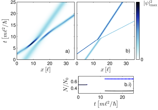
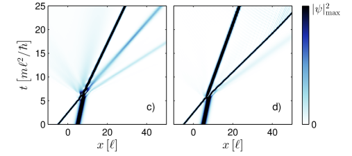
Figure 1: (colour online). High-velocity collisions of two co-moving chiral solitons. (a)-(b) Trajectories of inelastic interactions with $g_{\mathrm{1D}}m\ell/\hbar^{2}=0$, $v_{1}m\ell/\hbar=2$, $v_{2}m\ell/\hbar=1$, and $\delta=0$, where the gauge field strength is $a_{1}/\hbar=1$ in (a), and $a_{1}/\hbar=4$ in (b). (c)-(d) Soliton fission with $g_{\mathrm{1D}}m\ell/\hbar^{2}=2$, $v_{1}m\ell/\hbar=2$, $v_{2}m\ell/\hbar=0.5$, $a_{1}/\hbar=5$, with $\delta=0$ (c), and $\delta=\pi$ (d). b.i) Populations of the soliton envelopes before and after the collision pictured in b), highlighting the population transfer.

The colourbar limit has been intentionally lowered in (c)-(d) to display the solitons more clearly.

In each case, the interaction induced by the current nonlinearity dominates over the usual mean-field effects due to the solitons’ high velocities, which effectively reduces the mean-field scattering parameter. Figure 1(a) and Fig. 1(b) highlight extreme manifestations of this regime, where the dynamics are solely influenced by the current nonlinearity, setting $g_{\mathrm{1D}}m\ell/\hbar^{2}=0$, i.e., the mean-field contact interaction is completely disregarded.

Surprisingly, the collisions in these two instances are similar to those produced by the conventional NLS dynamics, with the solitons surviving the collision and retaining the general shape of their envelopes. However, two key differences are visible in the trajectories of the solitons, particularly in the case of $a_{1}/\hbar=4$, Fig. 1(b). The first are a pair of inelastic trajectories, with velocities of the outgoing solitons differing from their initial velocities, with the left- and right-most solitons reducing and increasing their velocities, respectively. The second difference from the mean-field setting is the appearance of a density node at the interaction centre, which is reminiscent of a repulsive interaction, despite the initial phase difference taken as $\delta=0$, which is conventionally an attractive interaction (for the solitons colliding in-phase). A third feature is also spotted in the form of population transfer, as illustrated in the Fig. 1(b.i) for the collision pictured in Fig. 1(b). Here, approximately a quarter of the initial mass of the right-most soliton is transferred to the left-most soliton in the course of the collision. Note, that the populations of the solitons are not calculated during the collision at $(\hbar/m\ell^{2})t=4$ to $(\hbar/m\ell^{2})t=12$, due to the overlap of the soliton envelops.

Each of these effects can be traced to the non-integrability of the current nonlinearity, which permits the transfer of stored interaction energy into the kinetic energy, and a possibility of a non-trivial shift of the soliton phase difference. The presence of the population transfer is directly linked to the phase shift, as both quantities are mutually conjugate. The energy exchange, or, to a greater extent, the inelasticity of the collision, appears to be minimised when the collision parameters are chosen so that the solitons interact repulsively. This is evident from comparisons between the two figures, where we note that $a_{1}/\hbar=1$ leads to a repulsive interaction with elastic trajectories, while $a_{1}/\hbar=4$ gives rise to a more attractive interaction which features inelastic trajectories.

The lower row of Fig. 1 shows the dynamics where the collision is destructive, causing fission of the solitons. In both cases, three solitons emerge from the collision (the third soliton in Fig. 1(d) with $\delta=\pi$ is located at the leading edge of the other two) with the populations and velocities of each outgoing soliton depending on the initial phase difference. In addition, a modest amount of radiation is ejected during the collision, as seen in the trailing edge in Fig. 1(c), and the interference pattern located between the slowest two solitons in Fig. 1(d). The main difference against the previous case is a larger difference in the initial velocities, which, if coupled with a larger gauge-field strength, $a_{1}/\hbar=5$, produces two soliton envelopes with a greater disparity of widths. As such, in the course of the collision, the solitons effectively interact over a longer period, thus enhancing effects stemming from the interaction.

III.2 Weak interactions

In the previous subsection it was seen how chiral solitons undergo inelastic collisions. To quantify the elasticity of the collisions, we introduce the coefficient of restitution fusfis1

$$\eta=\frac{\left(m_{1}v_{1}^{2}+m_{2}v_{2}^{2}\right)_{f}}{\left(m_{1}v_{1}^{2}+m_{2}v_{2}^{2}\right)_{0}},$$ (19)

which compares the difference of the kinetic energy before and after the collision. For $\eta=1$, the collision is perfectly elastic with conserved masses and velocities of the solitons, while $\eta\neq 0$ indicates an inelastic collision. Here, $m_{1,2}$ and $v_{1,2}$ play the role of the masses and velocities of the solitons in our semi-classical description, and are calculated from the respective expectation values,

$$m_{1,2}=m\langle N_{1,2}\rangle=m\int dx|\psi|^{2},$$ (20)

$$v_{1,2}=\langle\hat{p}_{1,2}\rangle/m_{1,2}=-\frac{i\hbar}{m_{1,2}}\int dx\psi^{\ast}\partial_{x}\psi.$$ (21)

The integration in each case at either the initial or final time is performed locally around each soliton’s centre of mass to exclude contributions from radiation and overlap with the other soliton. Due to the occurrence of both the population transfer and changes in the outgoing velocities of the solitons, one cannot distinguish whether the chiral solitons pass through or rebound off each other during the collision. Therefore, to remain consistent, we denote the solitons located in the $x<0$ and $x>0$ regions as the first and second ones, respectively.

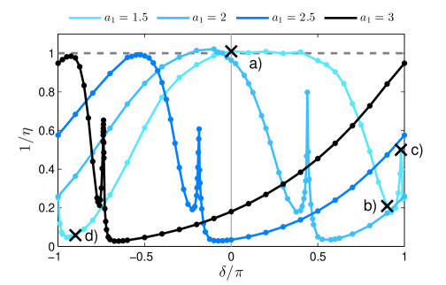
Figure 2: (colour online). Inverse of the coefficient of restitution calculated from numerical simulations (dots), with $g_{\mathrm{1D}}m\ell/\hbar^{2}=-4$, $v_{1}m\ell/\hbar=0.1$, and $v_{2}m\ell/\hbar=0$. The grey dashed line indicates the standard GPE results with perfectly elastic collisions, black crosses corresponding to the simulations in Fig. 3.

By varying the strength of the gauge field, we have performed a detailed parameter scan of the soliton-soliton collisions as a function of the initial phase difference, with the initial soliton velocities fixed. The coefficient of restitution is computed and plotted in Fig. 2 with corresponding examples of the dynamics shown in Fig. 3.

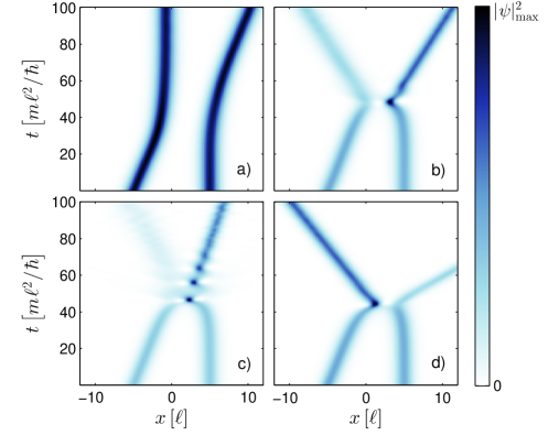
Figure 3: (colour online). Asymmetric collisions between two chiral solitons for various phase differences. The soliton parameters are $g_{\mathrm{1D}}m\ell/\hbar^{2}=-4$, $v_{1}m\ell/\hbar=0.1$, $v_{2}m\ell/\hbar=0$, and $a_{1}/\hbar=1.5$. The phase differences are taken as $\delta=0$ (a), $\delta=0.9\pi$ (b), $\delta=0.98\pi$ (c), and $\delta=-0.9\pi$ (d).

For each value of the gauge-field strength, three regimes of the collision dynamics can be identified, depending on the initial phase difference between the solitons. The first is an elastic scattering regime highlighted by a plateau in the restitution data at $\eta=1$, with an example of the dynamics shown in Fig. 3(a). Here, the interaction is notably repulsive, with a distinct node in the density at the interaction centre and the soliton parameters keeping their values after the collision.

Away from this plateau, two distinct regimes of inelastic dynamics are found with $\eta>1$, as illustrated in Fig. 3(b) and Fig. 3(d). Here, the dynamics are also similar to the case of strong interactions, with inelastic trajectories that feature a redistribution of the soliton masses, as well as evolution of the initial phase difference, resulting in shifts of the in- and out-of-phase collision points. Comparing these two plots, one notices that, depending on the direction in which one moves away from the plateau in the parameter space, the soliton mass can be transferred, chiefly, in either the left (Fig. 3(d)) or right-hand (Fig. 3(b)) outgoing soliton.

The final inelastic regime, indicated by the ‘resonance’ peak in the restitution data represented by the cross labelled (c) in Fig. 2), features the turning point of this population transfer, where the mass is transferred from one soliton to the other. We show in Fig. 3(c) an example of the dynamics in this regime, at the maxima of the ‘resonance’ peak. Here, a peculiar soliton state is formed, where there is a strong interplay between emitted radiation, excitation of an oscillatory mode in the right-hand soliton, and a weak left-hand one. This regime appears to be an example of in-phase (fully attractive) dynamics, which features the formation of a metastable (short-lived) bound state.

A feature universal to the restitution data presented in Fig. 2 is that the location of each inelastic regime is cyclically shifted left-wards for an increasing current strength. Comparing different gauge-potential strengths, one can see that the elastic region shrinks for larger values, which can be explained by enhancement of the non-integrability effects for stronger gauge-field strengths. Although not shown here, the dip in the restitution data initially appears close to $\delta=0$ at small values of the current strength, and cyclically displaces towards lower $\delta$ for increasing current strengths.

To complete the analysis for the weak-chiral regime, we perform a similar parameter scan as before, but now in the case when the relative phase difference is fixed to $\delta=0$, with the initial velocity of the left-hand soliton allowed to vary. In this case, the coefficient of restitution provides a poor illustration of the underlying dynamics, therefore we, instead, plot the outgoing velocity of the soliton travelling to the right for increasing values of the gauge-field strength, as shown in Fig. 4(a).

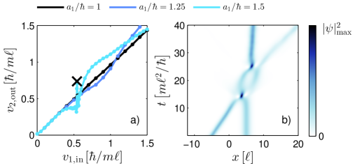
Figure 4: (colour online). (a) Outgoing versus incoming velocities for asymmetric collisions between two chiral solitons for various gauge-field strength, with parameters $g_{\mathrm{1D}}m\ell/\hbar^{2}=-4$, $v_{2}m\ell/\hbar=0$, and $\delta=0$ fixed in each instance. Black cross indicates the two-bounce resonance state shown in (b) for $v_{1}m\ell/\hbar=0.5425$ and $a_{1}/\hbar=1.5$.

Depending on the choice of the initial velocity and gauge-field strength, the strength of the chiral interactions $|a_{1}(v_{1}+v_{2})|$ may be either small or comparable to the mean-field strength $|g_{\mathrm{1D}}|$. Therefore, for extreme values of the parameters, it is expected that the dynamics will be generally inelastic in a similar manner to Fig. (1), whereas for smaller values the dynamics will be, generally, elastic. This reasoning is reflected in the pair of curves corresponding to $a_{1}/\hbar=1$ and $a_{1}/\hbar=1.25$ in Fig. 4(a), in which the soliton velocity does not change significantly after the interaction for small initial velocities. As the velocity increases (and hence the interaction strength increases too), this invariance begins to break, which is particularly notable in the case of $a_{1}/\hbar=1.25$, which exhibits a sinusoidal behaviour, at the velocity exceeding a critical value, $v_{1}\approx 0.5$.

As the gauge field strength is increased further, as in the case of $a_{1}/\hbar=1.5$, a ‘resonance’ feature appears in the data where a two-bound resonance state is formed, as shown in Fig. 4(b). As mentioned previously, such states are a common occurrence in non-integrable models chaos1 ; chaos2 ; chaos4 ; chaos5 ; chaos6 ; chaos7 ; chaos8 ; chaos9 ; chaos10 ; chaos11 , perhaps most notably in non-integrable versions of the sine-Gordon equation chaos11 , where, depending on the strength and shape of the interaction potential, an $n$-bound resonance state may emerge. Here the underlying mechanism is the energy exchange between the colliding solitons as a whole and their internal modes, which requires the solitons to collide several times before escaping, thus regaining the energy temporarily transferred into the internal mode. In performing this parameter scan, higher-order bound states, where the solitons collide more than twice, were not observed, as for stronger interaction strengths the appearance of a bound state tends to be suppressed in a similar manner to Fig. 3(c).

III.3 Bound states

To further investigate the inelastic dynamics of the density-dependent gauge theory, we consider a set of symmetric collisions (see Fig. 5), where two interacting solitons form a molecule-like bound state.

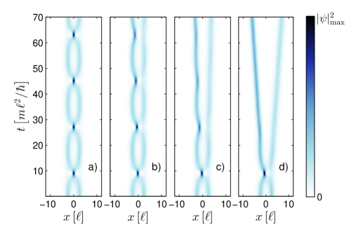
Figure 5: (colour online). Breakdown of the soliton-soliton bound state due to the presence of the current nonlinearity. Two stationary solitons are initially placed at distance $x/\ell=5$ units apart, with $g_{\mathrm{1D}}m\ell/\hbar^{2}=-4$ and $\delta=0$. The gauge-field strength varies as $a_{1}/\hbar=0$ (a), $a_{1}/\hbar=0.125$ (b), $a_{1}/\hbar=0.25$ (c), and $a_{1}/\hbar=0.5$ (d).

In a similar manner to results obtained in weakly perturbed cubic-quintic NLS chaos1 ; chaos10 and sine-Gordon systems chaos2 , a weak current nonlinearity is found to support short-lived bound states, where the solitons collide several times before escaping. As before, the underlying mechanism here is the transfer of a part of the energy of the interaction between the solitons into the kinetic energy and redistribution of the soliton masses. However, the magnitude of the interaction energy is now comparable to or larger than the kinetic energy of the solitons, requiring them to collide several times in order to gain enough kinetic energy for escaping the attractive interaction. Compared to the standard Gross-Pitaevskii dynamics shown in Fig. 5(a) with $a_{1}/\hbar=0$, where the solitons are perpetually trapped with a fixed oscillation amplitude and frequency, a modest current strength can begin to destabilize the bound state, such as in Fig. 5(c) for $a_{1}/\hbar=0.25$, where the solitons collide four times before escaping, and in Fig. 5(d) for $a_{1}/\hbar=0.5$, where they collide twice before escaping.

Interestingly, despite the interaction being initially symmetric, effects stemming from the chiral dynamics result in a left-handedness in the post-collision behaviour. For example, in Fig. 5(b) with $a_{1}/\hbar=0.125$, the first collision at $(\hbar/m\ell^{2})t=10$ is noticeably attractive due to the presence of the anti-node at the interaction centre, but every subsequent collision becomes increasingly repulsive with the amplitude of the anti-node decreasing and its position shifting towards the left. In addition, a density node fills the vacancy left by the anti-node at each interaction centre, with some manifestation of the population transfer. This effect is seen to be most profound in Fig. 5(d) for $a_{1}/\hbar=0.5$, where $\sim 60\%$ of the outgoing mass in captured in the left soliton. Returning to the two-bound resonance state in Fig. 4, the existence of higher-order bound states appears unlikely due to the fact that each subsequent interaction becomes more repulsive, hence more elastic than the previous one. These dynamics highlight the role that the lack of the Galilean invariance plays in the interacting gauge theory. In particular, the current operator appearing in Eq. (10) induces the population transfer between the two solitons, resulting in the suppression and, ultimately, breakdown of the bound state.

IV The variational analysis

To gain insight into how the current nonlinearity modifies the interactions between the solitons, we have performed variational calculations to derive an effective particle model for the soliton dynamics. We achieve this by using two similar, but essentially different methods.

In the first instance, we approximate the two-soliton state as a linear superposition of two individual solitons, with the interaction treated as the spatial overlap of the soliton envelopes. This technique has been previously applied to interaction problems in the NLS solint2 ; solint3 and Gross-Pitaevskii equations solint4 ; solint6 , in addition to several others solint1 ; solint5 ; solint7 ; solint8 ; solint9 . An advantage of this method is the ability to derive a set of variational equations which describe the motion of the solitons. From this, two key results can be extracted. The first is an effective potential describing the interaction between the solitons, which will provide details into the phase dependence and range of the interactions. Secondly, by numerically solving the variational equations, we will be able to illustrate the dynamics of the particle model and compare it directly to the full numerical solutions that are presented above.

For the second method, we follow the technique outlined in Refs. boris1 ; boris2 , in which the soliton state is also approximated as a linear superposition, but restricted to the case of two stationary solitons which are well-separated. In this case, the interaction is accounted for by the spatial overlap of one soliton with the ‘weak tail’ of the other, and may therefore be regarded as an asymptotic approximation to the full interaction. As such, this method is well suited to the study of bound states, but will also provide a basis to draw comparisons to the first method in a far-field low-velocity limit.

IV.1 Linear calculations

The starting point for the variational calculation is the Lagrangian density anyon ; zoller

$$\begin{split}\mathcal{L}&=\frac{i}{2}\left(\tilde{\psi}\partial_{\tilde{t}}\tilde{\psi}^{\ast}-\tilde{\psi}^{\ast}\partial_{\tilde{t}}\tilde{\psi}\right)+\frac{1}{2}|\partial_{\tilde{x}}\tilde{\psi}|^{2}+\frac{\tilde{g}_{\mathrm{1D}}}{2}|\tilde{\psi}|^{4}\\ &+\tilde{a}_{1}|\tilde{\psi}|^{2}\frac{d}{d\tilde{t}}\int_{-\infty}^{\tilde{x}}d\tilde{x}^{\prime}|\tilde{\psi}\left(\tilde{x}^{\prime},\tilde{t}\right)|^{2},\end{split},$$ (22)

where we have introduced dimensionless variables $x=\tilde{x}\ell$, $t=\tilde{t}m\ell^{2}/\hbar$, $\psi=\tilde{\psi}/\sqrt{\ell}$, $g_{\mathrm{1D}}=\tilde{g}_{\mathrm{1D}}\hbar^{2}/m\ell$, and $a_{1}=\tilde{a}_{1}\hbar$, with the length scale $\ell$. Here, and in the remainder of this paper, we drop the tildes appearing in these variables, working in the dimensionless units.

In what follows, we seek stationary solutions determined by the action

$$\begin{split}\mathcal{S}\left[q_{n}(t)\right]&=\int_{t_{1}}^{t_{2}}dt\int_{-\infty}^{\infty}dx\mathcal{L}(q_{n}(t),\dot{q_{n}}(t))\\ &=\int_{t_{1}}^{t_{2}}dt\langle\mathcal{L}\rangle,\end{split}$$ (23)

which gives rise to the Euler-Lagrange equations for each variational parameter $q_{n}(t)$, namely,

$$\frac{\partial\langle\mathcal{L}\rangle}{\partial q_{n}}-\frac{d}{dt}\frac{\partial\langle\mathcal{L}\rangle}{\partial\dot{q_{n}}}=0.$$ (24)

The variational ansatz is adopted as

$$\psi=\sum_{j=1,2}a\operatorname{sech}\left((x-\xi_{j})/b\right)e^{iS_{j}},$$ (25)

in which each soliton contains a spatially-varying phase solansatz1 ; solansatz2 ,

$$S_{j}=v_{j}\left(x-\xi_{j}\right)+\phi_{j}.$$ (26)

Here, $a(t)$, $b(t)$, $\xi_{j}(t)$, $v_{j}(t)$, and $\phi_{j}(t)$ are time-dependent variational parameters corresponding to the amplitude, width, centre-of-mass coordinates, velocities, and central phases of the solitons. This ansatz models two bright solitons in which the individual velocities and positions are allowed to evolve independently, with the interaction treated as the (linear)-overlap of the soliton envelopes. The constraint that the solitons have a common width, which in turn fixes the profiles of the soliton envelopes, is a necessary restriction in order to be able to explicitly calculate interaction integrals. Consequently, this restricts the variational analysis to the regime in which

$$\frac{b_{1}}{b_{2}}=\frac{g_{\mathrm{1D}}-2a_{1}v_{2}}{g_{\mathrm{1D}}-2a_{1}v_{1}}\approx 1.$$ (27)

This can be achieved by considering collisions with small velocities and by compensating the effects of the gauge field by a mean field with a modest strength, such that $|a_{1}(v_{1}+v_{2})|\ll|g|$. Therefore, the above constraint restricts our variational analysis to the weak-chiral regime for which numerical results are presented above. In spite of these restrictions, we will find that one may be quite liberal with the choice of parameters and still achieve sensible results.

Our choice of ansatz arises due to two reasons. First, our model is non-integrable, therefore a closed-formed expression for a two-soliton state via inverse scattering techniques is not available. Secondly, regardless of whether such a solution existed, Eq. (25) should work as a good approximation to the dynamics pictured in Fig. (3), as the solitons roughly retain their shape during the interaction. However, it must be stressed that this choice of the ansatz does not fully replicate all the features of the interaction and will therefore lead to inconsistencies at short length scales, when the solitons begin to significantly overlap.

An important example of this which must be considered before proceeding, is related to a divergence of the soliton amplitude $a(t)$ at short length scales. This can be illustrated by evaluating Eq. (15) for our variational ansatz, from which one can obtain the following expression for the soliton’s amplitude:

$$a^{2}=\frac{1}{4b}\frac{1}{1+\epsilon\operatorname{csch}(\epsilon)\cos(\delta)}=\frac{1}{4b}\frac{1}{f(\epsilon,\delta)}.$$ (28)

To perform the integration, we have introduced the change of variables $\alpha=(x-\xi_{1})/b$ and $\alpha+\epsilon=(x-\xi_{2})/b$, where $\epsilon=(\xi_{1}-\xi_{2})/b$ is a new variational parameter describing the relative positions of the solitons. Additionally, we have assumed that the magnitude of the velocity is small, such that the phase difference $S_{1}-S_{2}\approx\delta$ is an approximate function of solely the central phases. Additional details of the calculation are outlined in Appendix. A. Although this integral can be evaluated exactly without needing this approximation solint3 , the ensuing exact expression is to cumbersome for extracting explicit results from it. Inspecting Eq. (28), one can see that, in the limit of $\epsilon\rightarrow 0$, the value of $a^{2}(t)$ rapidly diverges for $\delta\in[\pi/2,3\pi/4]$ and approaches a singularity at $\delta=\pi$, modulo $2\pi$. Our approximations therefore lead to an unphysical divergence which is not representative of soliton collisions, thereby requiring us to restrict our studies to the bounded domain $|f(\epsilon,\delta)|\geq 1$, which corresponds to the interval of $\delta\in[0,\pi/2]$. For such values of $f$ which are bounded from below, $a(t)$ is non-divergent, representing the known dynamics more adequately—for instance, at $\delta=0$, which corresponds to the fact that the solitons’ amplitude is increased by $1/\sqrt{2b}$ when they constructively interfere.

Substituting our ansatz into Eq. (22) and integrating via Eq. (23) leads to the averaged Lagrangians

$$\langle\mathcal{L}_{0}\rangle=2a^{2}b(\dot{\phi}_{1}+\dot{\phi}_{2})+\frac{4a^{4}bg^{\prime}_{2}}{3}+\frac{2a^{2}}{3b}-2a^{2}b(v_{1}\dot{\xi}_{1}+v_{2}\dot{\xi}_{2})+a^{2}b(v_{1}^{2}+v_{2}^{2}),$$ (29)

and

$$\begin{split}\langle\mathcal{L}_{I}\rangle&=2a^{4}bg^{\prime}_{2}\left(1+\cos(2\delta)/2\right)\left[\frac{4\epsilon\cosh(\epsilon)}{\sinh^{3}(\epsilon)}-\frac{4}{\sinh^{2}(\epsilon)}\right]+\frac{a^{2}}{b}\cos(\delta)\left[\frac{4\cosh(\epsilon)}{\sinh^{2}(\epsilon)}+\frac{4\epsilon}{\sinh(\epsilon)}-\frac{4\epsilon\cosh^{2}(\epsilon)}{\sinh^{3}(\epsilon)}\right]\\ &+a^{2}(v_{1}+v_{2})\sin(\delta)\left[\frac{2\epsilon\cosh(\epsilon)}{\sinh^{2}(\epsilon)}-\frac{2}{\sinh(\epsilon)}\right]-a^{2}b^{2}\cos(\delta)\left(\dot{v}_{1}-\dot{v}_{2}\right)\left[\frac{\epsilon^{2}}{\sinh(\epsilon)}\right]\\ &+a^{2}b\cos(\delta)\left(v_{1}v_{2}-(v_{1}\dot{\xi}_{1}+v_{2}\dot{\xi}_{2})+\dot{\phi}_{1}+\dot{\phi}_{2}\right)\left[\frac{2\epsilon}{\sinh(\epsilon)}\right]+4a^{4}bg^{\prime}_{2}\cos(\delta)\left[\frac{2\cosh(\epsilon)}{\sinh^{2}(\epsilon)}-\frac{2\epsilon}{\sinh^{3}(\epsilon)}\right],\end{split}$$ (30)

where we have defined $g_{2}^{\prime}=g_{\mathrm{1D}}-a_{1}\left(v_{1}+v_{2}\right)$, and have split the total Lagrangian into the sum of terms which implicitly and explicitly depend on $\epsilon$, as denoted by the free and interacting Lagrangians, $\mathcal{L}=\mathcal{L}_{0}+\mathcal{L}_{I}$.

Equations of motion for each variational parameter can now be derived from Eq. (24), which lead to the set of coupled differential equations

$$\phi_{i}:\quad\quad\partial_{t}\left(4a^{2}bf\left(\epsilon,\delta\right)\right)=0,$$ (31)

$$v_{i=1(+),2(-)}:\quad\quad v_{i}=\dot{\xi}_{i}l_{i}\left(\epsilon,\delta\right)+\frac{4a^{2}a_{1}}{6}+d\left(\epsilon,\delta\right)-v_{i\pm 1}\cos(\delta)\frac{\epsilon}{\sinh(\epsilon)},$$ (32)

$$a:\quad\quad\left.\frac{\partial\langle\mathcal{L}\rangle}{\partial a}\right|_{\dot{q}_{n}}+4ab\sum_{n=1,2}\left(\dot{\phi}_{n}-v_{n}\dot{\xi}_{n}\right)f(\epsilon,\delta)=2ab^{2}\left(\dot{v}_{1}-\dot{v}_{2}\right)\cos(\delta)\frac{\epsilon^{2}}{\sinh(\epsilon)},$$ (33)

$$\xi_{i}:\quad\quad\left.\frac{\partial\langle\mathcal{L}_{I}\rangle}{\partial\xi_{i}}\right|_{\dot{q}_{n}}+2a^{2}b\frac{\partial f}{\partial\xi_{i}}\sum_{n=1,2}\left(\dot{\phi}_{n}-v_{n}\dot{\xi}_{n}\right)=-2\partial_{t}\left(a^{2}bv_{i}f(\epsilon,\delta)\right)+a^{2}b^{2}\left(\dot{v}_{1}-\dot{v}_{2}\right)\partial_{\xi_{i}}\frac{\epsilon^{2}}{\sinh(\epsilon)},$$ (34)

with

$$\begin{split}d\left(\epsilon,\delta\right)&=4a^{2}a_{1}\left(\left(1+\frac{\cos(2\delta)}{2}\right)\left[\frac{\epsilon\cosh(\epsilon)}{\sinh^{3}(\epsilon)}-\frac{1}{\sinh^{2}(\epsilon)}\right]+\cos(\delta)\left[\frac{\cosh(\epsilon)}{\sinh^{2}(\epsilon)}-\frac{\epsilon}{\sinh^{3}(\epsilon)}\right]\right)\\ &-\frac{\sin(\delta)}{b}\left[\frac{\epsilon\cosh(\epsilon)}{\sinh^{2}(\epsilon)}-\frac{1}{\sinh(\epsilon)}\right],\end{split}$$ (35)

and

$$l\left(\epsilon,\delta\right)_{i=1(+),2(-)}=1+\cos(\delta)\frac{\epsilon}{\sinh(\epsilon)}\mp\frac{1}{2a^{2}b}{\partial}_{\xi_{i}}\left(a^{2}b^{2}\cos(\delta)\frac{\epsilon^{2}}{\sinh(\epsilon)}\right).$$ (36)

Here, the vertical bar notation in Eqs. (33-34), denotes the full Lagrangian function in Eq. (30), but excluding terms containing a factor of $\dot{\phi}_{i}$, $\dot{\xi}_{i}$, or $\dot{v}_{i}$. In Eqs. (32) and (36), for $i=1$ positive (+) operations are taken, with the converse for $i=2$. A variational equation for $b$, the solitons’ width, is not required to proceed and is excluded. Both Eqs. (35) and (36) are introduced for notational convenience. From the set of variational equations, we can now extract details of how the gauge field affects the soliton dynamics, and derive several important quantities.

Starting with the first variational equation, which can be obtained by varying either $\phi_{1}$ or $\phi_{2}$, one can identify Eq. (31) as a conservation law for $4a^{2}bf(\epsilon,\delta)$. This is consistent with both Eqs. (15) and (28), which state that the phase and density of the condensate are conjugate variables. In the asymptotic limit of $\epsilon\rightarrow\infty$, this conserved quantity reduces to $a^{2}\sim 1/4b$, which is the correct amplitude for a two-soliton state.

The equations for the velocities $v_{i}$ highlight the main result of the variational analysis. The first and last terms of Eq. (32) (and the last term of Eq. (35)), correspond to similar terms in the NLS equation. Together they imply that, in the asymptotic limit of $v_{i}\sim\dot{\xi_{i}}$, both solitons move at a constant velocity when they are well separated. However, at $\epsilon\rightarrow 0$ the velocities of the solitons are modified due to their interaction, but, once again, they become constant after the solitons have passed through each other. The additional terms $\propto a_{1}$, which appear in the velocity equation, are new ones, which arise due to the presence of the gauge potential. The first of these is a non-Galilean effect that redefines the soliton velocities in the asymptotic limit as $v_{i}\sim\dot{\xi}+a_{1}/6b$, which is consistent with the momentum conservation law stated in Eq. (16). The remaining terms which appear in Eq. (35) are responsible for the interaction-induced velocity shift, which, in both the $v_{1}$ and $v_{2}$ equations, has the same magnitude and sign.

The variational equations for both $a$ and $\xi_{i}$ are not particularly transparent. However, they do highlight the coupling between all of the variational parameters, and will be required when deriving the interaction potentials later in the section.

IV.1.1 Collision dynamics

In order to illustrate how the gauge field is the mechanism underlying the inelastic scattering in our system, we set out to first simplify and reduce the number of variational equations, so that an effective particle model can be derived. Subsequently, we can numerically solve our system of equations and compare it to the full numerics presented above.

We begin by first reiterating that we consider the case of weak-chiral interactions $|a_{1}(v_{1}+v_{2})|\ll|g|$, which feature the solitons moving slowly for a given choice of the gauge-field strength. Equations (33-34) may then be set up as a set of simultaneous equations in which coordinates, $\dot{\phi}_{1}$, $\dot{\phi}_{2}$, $\dot{\xi}_{1}$, and $\dot{\xi}_{2}$ can be eliminated, leading to a pair of equations

$$\dot{v}_{1}\gamma+\dot{v}_{2}\left(\gamma-1\right)=-4\left.\frac{\partial\langle\mathcal{L}_{I}\rangle}{\partial\xi_{1}}\right|_{\dot{q}_{n}},$$ (37)

$$\dot{v}_{2}\gamma+\dot{v}_{1}\left(\gamma-1\right)=-4\left.\frac{\partial\langle\mathcal{L}_{I}\rangle}{\partial\xi_{2}}\right|_{\dot{q}_{n}},$$ (38)

with $\gamma\equiv 1-(b/2)\partial_{\xi_{1}}\left(\epsilon\left(f-1\right)/f\right)$. Together with Eq. (32), they form a set of coupled differential equations for the soliton dynamics, in which details of the interaction are encoded in expressions for $\gamma(\epsilon,\delta)$ and $\langle\mathcal{L}_{I}\rangle$. Once again, in the asymptotic limit, both equations simplify to the single-soliton result $\dot{v}_{i}\sim 0$, which highlights that both solitons move independently at a constant velocity when they are well separated. A consequence stemming from the elimination of variables $\dot{\phi_{1}}$ and $\dot{\phi_{2}}$ in the equations highlights that the phase in this particle model is static, and does not dynamically evolve. Although this is an important feature in our model which has many consequences in the scattering dynamics, we will still be able to obtain qualitative results which do not strongly depend on phase $\delta$, but will not be able to address issues pertaining to the bound-states dynamics pictured in Fig. 5.

We solve the set of differential equations numerically using a fourth-order Runge-Kutta method and compare our results to an example of the full numerics in Fig. (6).

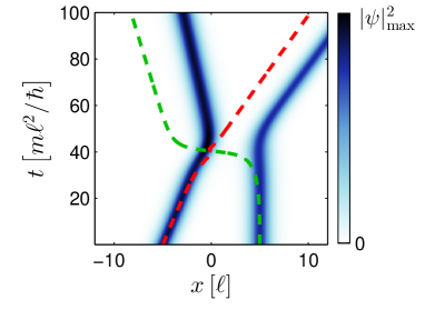
Figure 6: (colour online). Comparison between the solutions of the variational equations (dashed-green/red) and full numerics (blue) for the evolution of the solitons’ centres of mass. The soliton parameters are taken as $g_{\mathrm{1D}}=-4$, $v_{1}=0.1$, $v_{2}=0$, $a_{1}=3$, and $\delta=0.4\pi$.

For the chosen set of parameters, the magnitude of the outgoing velocities are in good agreement with the post-collision trajectories showing that the solitons pass through each other. However, position shifts of the solitons are not captured well, with the left-outgoing soliton shifted too much, and the right-outgoing soliton shifted too little. This particular example represents the configuration that has the best agreement for the velocities. Although not shown here, for $\delta<0.3\pi$ the particle model predicts that the solitons form a perpetual bound state with a centre of mass coordinate that increases linearly with time. Otherwise, for $\delta>\pi/2$, the dynamics feature a hard-core elastic interaction where the solitons collide, but rebound off each other. Although the dynamics in these two regimes are similar to what we have obtained numerically, in that we can identify regimes where the interaction is repulsive (and therefore elastic) and attractive (supporting bound states), this correlation actually arises from discrepancies in our model.

To explain how these discrepancies appear in our results, we restate the consequences of the various approximations that we have used in the analysis. In effect, all inconsistencies can be traced back to the initial ansatz used in the analysis, see Eq. (25). The first problem is the obvious fact that the ansatz is a linear superposition of two solitons, neglecting the nonlinear deformation which takes place when they overlap significantly. For this reason, important details of the interaction are omitted.

The second discrepancy in the ansatz, arises from the need to fix and equate the soliton widths. For two chiral solitons to interact, their velocities, and therefore, by extension, their widths, must be different. Furthermore, as the solitons’ velocities can change after colliding, $b(t)$ is a time-dependent quantity that requires the additional term $w\left(x-\xi_{i}\right)^{2}$ in the expression for the phase given by Eq. (26), with $w$ being the chirp. Although this was derived, it was eventually excluded due the complexity in implementing it in the particle model. The net result is that interaction effects in our particle model are isotropic with respect to each soliton’s mutual influence, which is clearly not the case in the full numerics.

Another inconsistency is the divergence of the amplitude Eq. (28) for short length scales in the regime of $\delta>\pi/2$. This artifact enters due to approximating the phase difference as a function of only the central phases, therefore neglecting velocity contributions. Although this was justified by taking the velocities small, the spatially-varying form of this phase is required to obtain sensible results, as was shown in solint3 . Due to the divergence of the amplitude, the effective interaction potential between the solitons also diverges in this regime, as we will demonstrate in the following subsection.

The final discrepancy takes place due to the static nature of the phase in our model. As was demonstrated in our simulations, the current nonlinearity introduces the population transfer and shifts in the soliton’s central phase at each collision. The absence of these properties in the model results, therefore, in the existence of perpetual bound states, in addition to the lack of changes in the soliton’s amplitudes/widths due to the populations transfer.

From this, it is sensible to conclude that the variational analysis presented here is more suited to studying dynamics at the onset of the collision, before the soliton envelopes significantly overlap, but not in the course of the collision proper.

IV.1.2 The interaction potential

The set of coupled differential equations can be reformulated into a mechanical system, in order to derive an effective potential describing the interaction between the solitons. We begin by first restricting our analysis at the onset of the collision, before the solitons began to significantly overlap, as said above. In this regime, the second soliton remains approximately stationary and we can fix that $\xi_{2}(t)=0$ and $v_{2}(t)=0$. The set of coupled differential equations then greatly simplify, and we may readily integrate Eq. (37) to obtain

$$v_{1}\dot{\xi}_{1}\gamma=-4\left.\langle\mathcal{L}_{I}\rangle\right|_{\dot{q}_{n}}+C,$$ (39)

where $C$ is an arbitrary integration constant. Substituting Eq. (32) into Eq. (39), and then substituting again to remove a factor of $\dot{\xi}_{1}$, leads to the mechanical energy equation,

$$\frac{1}{2}\dot{\xi}_{1}^{2}+\frac{a_{1}}{6bf^{2}\gamma}\dot{\xi}_{1}+V_{\mathrm{int}}=\frac{C}{2f\gamma^{2}},$$ (40)

where we identify the soliton kinetic energy $\dot{\xi}_{1}^{2}/2$, total energy $C/2f\gamma^{2}$, and the effective interaction potential,

$$V_{\mathrm{int}}=-\frac{1}{2f^{2}\gamma^{2}}\left[d\left(d+\frac{a_{1}}{6bf}-v_{1}\right)-4f\left.\langle\mathcal{L}_{I}\rangle\right|_{\dot{q}_{n}}\right].$$ (41)

The structure of Eq. (40), treats the motion of the first soliton as a classical particle moving through the potential landscape of the second.

We plot the interaction curves in Fig. 7, in comparison to an asymptotic calculation derived in the next section.

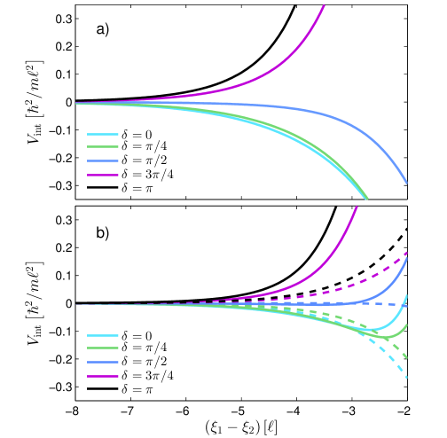
Figure 7: (colour online). (a) Potential-energy curves, predicted by Eq. (41) as a function of the soliton separation, for various phase differences. (b) Comparison between asymptotic curves obtained by Eq. (68) (solid) and Eq. (50) (dashed). In both cases, the parameters are taken as $g_{\mathrm{1D}}=-4$, $v_{1}=0.1$, and $a_{1}=3$.

The interaction curves are here plotted only for negative values of the separation, as we have considered the situation in which the moving soliton approaches the stationary soliton up to the start of the collision.

For a typical set of parameters which we have used in our simulations, the curves in Fig. 7 show that both repulsive and attractive interactions are supported, up to a choice of the phase difference. The presence of an attractive potential—in particular, for $\delta=0$ and $\delta=\pi/4$,—therefore supports the existence of bound states, and the interpretation of the ‘resonance’ regime in Fig. 2 as an example of the attractive dynamics. The effect of the divergence of the amplitude for $\delta>\pi/2$ is illustrated by the upper two curves of Fig. 7, as the magnitude of the potential increases rapidly.

In fact, the nature of these curves does not differ drastically from the results expected in the NLS equation, as contributions from terms stemming from the current feature as a short-range attractive potential, hence they do not have significant influence far from the centre of the interaction. This can be compared to the plot with $a_{1}=0$, from which it is well known that $\delta=0$, $\delta=\pi$, and $\delta=\pi/2$ correspond, respectively, to the attractive, repulsive, and weak intermediate interactions of solitons in the standard NLS equation.

IV.2 Asymptotic calculations

In the previous section, the interaction of two chiral solitons was explored using a full variational approach. It is further useful to consider an asymptotic approach for well-separated solitons. Such an analysis can be accomplished using the methodology presented in Refs. boris1 ; boris2 , where tails of the solitons are used to produce the interaction potential (see also other_method ). We begin by writing the one-dimensional Hamiltonian density for the system,

$$\mathcal{H}=-\frac{1}{2}|\left(\hat{p}-a_{1}|\psi|^{2}\right)\psi|^{2}-\frac{g_{\mathrm{1D}}}{2}|\psi|^{4},$$ (42)

which, when minimised, reduces to Eq. (7). To derive an effective interaction potential, we again restrict our analysis to the regime of weak-chiral interactions in which the second soliton can be taken as stationary with respect to the first. In addition, since $|a_{1}(v_{1}+v_{2})|\ll|g|$, we note that the dominant contributions to the interaction potential in Eq. (41) arise from terms not containing a factor of $v_{1}$. Therefore we can further impose that the first soliton is also stationary such that $v_{1}=v_{2}=0$. Then provided the solitons’ centres of masses are well separated by a distance $L=\xi_{1}-\xi_{2}$, we may approximate the two-soliton state in the vicinity of the first soliton as

$$\psi=\psi_{1}(x)+\psi_{2}(x+L),$$ (43)

in which $\psi_{1}$ represents the envelope of the first soliton, and $\psi_{2}$ is the exponential tail of the second soliton. The reciprocal approximation is valid in the region around the second soliton.

Next, we substitute Eq. (43) and its counterpart pertaining to the second soliton into Eq. (42), and retain terms which are linear with respect to the small tails, either $\psi_{1}$ or $\psi_{2}$. The resulting expression can be recast in a compact form as

$$\mathcal{H}_{12}=\left.\left[\psi_{2}\frac{\partial\mathcal{H}}{\partial\psi}+\partial_{x}\psi_{2}\frac{\partial\mathcal{H}}{\partial\psi_{x}}+\mathrm{c.c.}\right]\right|_{\psi=\psi_{1}},$$ (44)

where each derivative is evaluated at point $\psi=\psi_{1}$.

To proceed, we note that the Hamiltonian can be defined as $H=\int_{-\infty}^{+\infty}dx\mathcal{H}$, with the variational (alias Fréchet) derivative,

$$\frac{\delta H}{\delta\psi}=\frac{\partial\mathcal{H}}{\partial\psi}-\frac{\partial}{\partial x}\frac{\partial\mathcal{H}}{\partial\psi_{x}}.$$ (45)

As we consider only the case of exact solutions for which $\delta H/\delta\psi=0$, we may recast Eq. (44), using Eq. (45) and integration by parts, to obtain the expression

$$H_{12}=\left[\psi_{2}\left.\frac{\partial\mathcal{H}}{\partial\psi_{x}}+c.c\right]_{z_{0}}^{\infty}\right|_{\psi=\psi_{1}}+\{1\rightleftharpoons 2\},$$ (46)

which, after using Eq. (44), simplifies to

$$H_{12}=\left[\left(\frac{1}{2}\partial_{x}\psi_{1}^{\ast}{+}\frac{ia_{1}}{2}\psi_{1}^{\ast}|\psi_{1}|^{2}\right)\psi_{2}+\mathrm{c.c.}\right]_{z_{0}}^{\infty}{+}\{1\rightleftharpoons 2\}.$$ (47)

Rather than taking the integration limits in the domain $(-\infty,\infty)$, we here divide the integration domain at an arbitrary point $z_{0}$ located between the solitons, and introduce the symmetric contribution $\{1\rightleftharpoons 2\}$ to account for the contribution from the second soliton. To proceed, we require expressions for single-soliton states of Eq. (43), which are given by

$$\psi_{n}=\frac{1}{2\sqrt{b}}e^{i\phi_{n}}\times\begin{cases}\operatorname{sech}(x/b),&n=1,\\ \operatorname{sech}((x+L)/b),&n=2,\end{cases}$$ (48)

where the soliton’s width $b=-4/\tilde{g}$ is chosen such that $\sum_{n}\int_{-\infty}^{+\infty}dx|\psi_{n}|^{2}=1$, with each soliton containing half the number of atoms. In keeping with the linearisation procedure used in deriving Eq. (46), we can instead simplify these expressions in the vicinity of $z_{0}$, with asymptotic forms

$$\psi_{n}\sim\frac{1}{\sqrt{b}}e^{i\phi_{n}}\times\begin{cases}e^{-x/b},&n=1,\\ e^{\left(x+L\right)/b},&n=2.\end{cases}$$ (49)

To calculate the variational derivative in Eq. (45), we use the full expressions in Eq. (48) to evaluate the upper limit at $x=\infty$, together with the asymptotic forms in Eq. (49) to evaluate the lower limit at $z_{0}$. To obtain a contribution from the current to the effective potential, which is independent of the choice of arbitrary point $z_{0}$, we must go to the next order in the expression for $\psi_{2}$ in the second term in expression (47), taking $\psi_{2}\sim-\sqrt{2}e^{3\left(x+L\right)/b}e^{i\phi_{2}}/\sqrt{b}$. Substituting these expressions, we obtain an effective interaction potential

$$V_{\mathrm{int}}=-\frac{2}{b^{2}}\left[e^{\epsilon}\cos(\delta)+a_{1}e^{3\epsilon}\sin(\delta)\right],$$ (50)

which is convenient to extract information from. The first term in Eq. (50) comes from the NLS equation, being attractive/repulsive for the correct choice of $\delta$. The second term, which appears due to the current, may also be attractive or repulsive, but it is out of phase with the first term. However this term yields a shorter interaction range, compared to the NLS term, hence it does not contribute significantly to the interaction potential far from the centre of the interaction.

It is relevant to compare the interaction potentials produced by both the linear-superposition and asymptotic models. Because the asymptotic calculation neglects some terms in the underlying Hamiltonian density, compared to the linear-superposition ansatz (25), it is necessary to approximate the result produced by the linear superposition, using the asymptotic forms, so that they can be fairly compared. This is detailed in Appendix B. Figure 7 shows a comparison between these interaction potentials, from which we can see that both curves share the same qualitative features, with both repulsive and attractive interactions supported in a similar manner to the standard NLS equation.

V Conclusion

We have demonstrated how the current nonlinearity introduces non-integrable effects in the collision dynamics of bright matter-wave solitons. Using the variational approximation, we have derived an effective particle model for the soliton dynamics, which helps to explain both inelastic scattering and the attractive/repulsive nature of the interactions. We have also derived effective potentials for the interaction between the solitons. We showed that the particle model is valid as long as the current nonlinearity is weak, similar to the situation in integrable models, where inherent symmetries of the system can be exploited solint3 . This fact implies that essential results may be produced by collisions between slowly moving solitons. For stronger interactions, the particle model breaks down due to the non-integrability. We observe, in particular, how the strong current-induced nonlinearity can destabilize bound states of solitons and also induce soliton fission, breaking two colliding solitons into several ones after the collision.

These concepts constitute a rich spectrum of dynamics which are interesting from the point of view of the fundamental nonlinear dynamics. In addition, the chiral properties of the quantum gas studied here may provide novel applications to atomtronics atomtronics and quantum transport. In such scenarios, careful consideration of the collision dynamics is needed.

VI Acknowledgements

R.J.D. acknowledges support from EPSRC CM-CDT Grant No. EP/L015110/1, M.J.E. acknowledges support from EPSRC Grant No. EP/M005127/1 and as an Overseas researcher under Postdoctoral Fellowship of Japan Society for the Promotion of Science, and P.Ö. acknowledges support from EPSRC grant No. EP/M024636/1. B.A.M. appreciates hospitality of the Institute of Photonics and Quantum Sciences at the Heriot-Watt University. The work of that author is supported, in part, by the joint program in physics between NSF and Binational (US-Israel) Science Foundation through project No. 2015616, and by the Israel Science Foundation through Grant No. 1286/17.

Appendix A Calculation of interaction integrals

In this appendix we show how to evaluate the interaction integrals which appear in the variational analysis, using the method of residues. These calculations can be found in the standard literature solint1 ; solint3 , but we recapitulate details here, to provide a basis for evaluating more complicated integrals.

A.1 Integral example I

The simplest interaction integral to evaluate is

$$I_{1}=b\int_{-\infty}^{+\infty}\frac{d\alpha}{\cosh(\alpha)\cosh(\alpha+\epsilon)}.$$ (51)

To proceed, we consider the following contour integral

$$\oint_{\mathcal{C}}f(z)dz=\oint_{\mathcal{C}}\frac{z}{\cosh(z)\cosh(z+\epsilon)}dz,$$ (52)

in which the contour path $\mathcal{C}$ forms a rectangular region in the complex plane, $z=\alpha+iy$, with dimensions $-R<\alpha<R$, $0<y<\pi$. The complex function $f(z)$ is analytic in the region except for a pair of (simple) poles at $z_{1}=i\pi/2$ and $z_{2}=i\pi/2-\epsilon$. These properties are illustrated in Fig. (8).

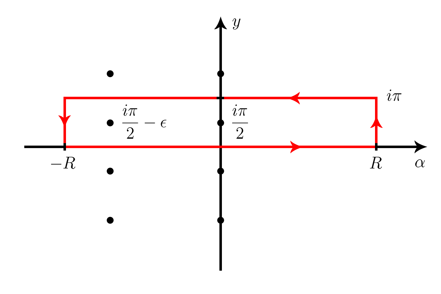
Figure 8: (colour online). Map of the complex plane $z=\alpha+iy$, highlighting the location of the poles (black dots) and contour path $\mathcal{C}$ (red line) for all interaction integrals. The integration path is counter-clockwise.

In the limit of $R\rightarrow\infty$, the contour integrals along the vertical paths vanish, as $f(z)$ exponentially converges to zero at $z=\pm\infty$. The horizontal paths also cancel, except for a contribution from the top path which is proportional to the desired integral. Therefore, from the residue theorem we can write

$$b\oint_{\mathcal{C}}f(z)dz=-i\pi I_{1}=2\pi ib\sum_{k=1,2}\text{Res}\left(f(z),z_{k}\right).$$ (53)

The task of evaluating $I_{1}$ reduces to simply, albeit tediously, computing the residues of $f(z)$, which are given by

$$\begin{split}\text{Res}\left(f(z),z_{1}\right)&=\lim_{z\rightarrow z_{1}}\left(z-z_{1}\right)f\left(z\right)\\ &=\frac{\pi}{2i\sinh(\epsilon)},\end{split}$$ (54)

$$\begin{split}\text{Res}\left(f(z),z_{2}\right)&=\lim_{z\rightarrow z_{2}}\left(z-z_{2}\right)f\left(z\right)\\ &=-\frac{\pi}{2i\sinh(\epsilon)}-\frac{\epsilon}{\sinh(\epsilon)}.\end{split}$$ (55)

Collating the results, we find

$$I_{1}=\frac{2b\epsilon}{\sinh(\epsilon)}.$$ (56)

A.2 Integral example II

A more involved example is

$$I_{2}=b\int_{-\infty}^{\infty}\frac{\alpha\tanh(\alpha+\epsilon)}{\cosh(\alpha)\cosh(\alpha+\epsilon)}d\alpha.$$ (57)

In this case, we consider the following contour integral:

$$\oint_{\mathcal{C}}g(z)dz=\oint_{\mathcal{C}}\frac{z^{2}\sinh(z+\epsilon)}{\cosh(z)\cosh^{2}(z+\epsilon)}dz,$$ (58)

in which the contour path $\mathcal{C}$ is identical to the one used in the previous example. In contrast, the integrand now contains a simple pole and a second-order one. Again, using the residue theorem, we can write

$$b\oint_{\mathcal{C}}g(z)dz=-2\pi iI_{2}+\pi^{2}I_{3}=2\pi ib\sum_{k=1,2}\text{Res}\left(g(z),z_{k}\right),$$ (59)

where the task of evaluating $I_{2}$ now depends on computing the residues of $g(z)$ and knowledge of the integral

$$\begin{split}I_{3}&=b\int_{-\infty}^{\infty}\frac{\tanh(\alpha+\epsilon)d\alpha}{\cosh(\alpha)\cosh(\alpha+\epsilon)}\\ &=-\frac{2b}{\sinh(\epsilon)}+\frac{2b\epsilon\cosh(\epsilon)}{\sinh^{2}(\epsilon)}.\end{split}$$ (60)

The residues in this instance are given by

$$\begin{split}\text{Res}\left(g(z),z_{1}\right)&=\lim_{z\rightarrow z_{1}}\left(z-z_{1}\right)g\left(z\right)\\ &=\frac{\pi^{2}\cosh(\epsilon)}{4\sinh^{2}(\epsilon)},\end{split}$$ (61)

$$\begin{split}\text{Res}\left(g(z),z_{2}\right)&=\lim_{z\rightarrow z_{2}}\frac{d}{dz}\left[\left(z-z_{2}\right)^{2}g\left(z\right)\right]\\ &=(i\pi-2\epsilon)\frac{1}{\sinh(\epsilon)}+\left(\epsilon-\frac{i\pi}{2}\right)^{2}\frac{\cosh(\epsilon)}{\sinh^{2}(\epsilon)}.\end{split}$$ (62)

Collating the results, we find

$$I_{2}=-\frac{b\epsilon^{2}\cosh(\epsilon)}{\sinh^{2}(\epsilon)}+\frac{2b\epsilon}{\sinh(\epsilon)}.$$ (63)

For the remaining interaction integrals, one can proceed using the same methodology, provided that the correct contour shift is applied to the integral, namely,

$$\int^{\infty}_{-\infty}f\left(\alpha,\epsilon\right)\alpha^{n-1}d\alpha\rightarrow\int_{\mathcal{C}}f\left(z,\epsilon\right)z^{n}dz,$$ (64)

or

$$\int^{\infty}_{-\infty}f\left(\alpha,\epsilon\right)\left(\alpha+\epsilon\right)^{n-1}d\alpha\rightarrow\int_{\mathcal{C}}f\left(z,\epsilon\right)\left(z+\epsilon\right)^{n}dz,$$ (65)

where $n\in\mathbb{Z}^{+}$ and $f(\alpha,\epsilon)$ is a product of hyperbolic functions.

Appendix B The asymptotic approximation for the interaction potential produced by the linear-superposition ansatz

To directly compare the interaction potentials derived from the variational analysis, it is necessary to reduce the potential obtained from the linear-superpositon ansatz (25) to a form which captures the same approximations which were used in the asymptotic version, based on ansatz (43). This can be done by introducing asymptotic forms for each contribution to the interaction potential and selectively dropping terms which are either short-range ones, or contain an explicit dependence on the soliton velocities.

We start, by explicitly restating the linear interaction potential

$$\begin{split}V_{\rm int}&=-\frac{1}{2(bf\gamma)^{2}}\left(d^{2}+\frac{a_{1}}{6bf}d\right)+\frac{g}{bf\gamma^{2}}\left(\left(1+\cos(2\delta)/2\right)\left[\frac{\cosh(\epsilon)}{\sinh^{3}(\epsilon)}-\frac{1}{\sinh(\epsilon)}\right]+\cos(\delta)\left[\frac{\cosh(\epsilon)}{\sinh^{2}(\epsilon)}-\frac{\epsilon}{\sinh^{3}(\epsilon)}\right]\right)\\ &+\frac{1}{b^{2}}\cos(\delta)\left[\frac{\cosh(\epsilon)}{\sinh^{2}(\epsilon)}+\frac{\epsilon}{\sinh(\epsilon)}-\frac{\epsilon\cosh^{2}(\epsilon)}{\sinh^{3}(\epsilon)}\right],\end{split}$$ (66)

which has been simplified by taking $v_{1}=0$, for the case of two stationary solitons. To reduce Eq. (66) to an asymptotic form, we recall that, while deriving Eq. (41), we considered the dynamics of the soliton travelling in the positive $x$-direction under the action of the effective potential induced by the second soliton. Therefore, we are required to approximate the interaction potential for negative values of $\epsilon$, with respect to the second soliton which is centered at $x=0$. Then, in the same manner as before, we introduce the following asymptotic forms: $\cosh(\epsilon)\sim e^{-\epsilon}/2$, $\operatorname{csch}(\epsilon)\sim-2\epsilon^{\epsilon}$, $f(\epsilon,\delta)\sim 1-2e^{\epsilon}\epsilon\cos(\delta)$, and

$$\gamma(\epsilon,\delta)\sim 1-\frac{\left(1-f\right)^{2}\left(1+\epsilon\right)-f\left(1-f\right)\left(2+\epsilon\right)}{2f^{2}}.$$ (67)

Substituting these expressions into Eq. (66), one arrives at the asymptotic potential

$$\begin{split}V_{\rm int}&\sim-\frac{2}{\left(bf\gamma\right)^{2}}\left(-\sin(\delta)\left(\epsilon+1\right)e^{\epsilon}-\frac{2a_{1}}{f}\left(1+\cos(2\delta)/2\right)\left(\epsilon+1\right)e^{2\epsilon}+\frac{a_{1}}{f\hbar}\cos(\delta)e^{\epsilon}\right)^{2}\\ &+\frac{2}{f\gamma^{2}}\left(-\frac{4g}{b}\left(1+\cos(2\delta)/2\right)e^{2\epsilon}+\frac{2}{b^{2}}e^{\epsilon}\cos(\delta)+\frac{g}{b}\cos(\delta)e^{\epsilon}\right).\end{split}$$ (68)

In writing Eq. (68), we have neglected term $\propto e^{3\epsilon}$ and the term $\propto a_{1}d\left(\epsilon,\delta\right)/6$ in Eq. (66), as they, being small in the asymptotic limit, do not essentially affect the result.

References

- (1) Scott A 2005 Encyclopedia of Nonlinear Science (Routledge)
- (2) Drazin P G and Johnson R S 1989 Solitons: an introduction (Cambridge University Press)
- (3) Yang J 2010 Nonlinear Waves in Integrable and Nonintegrable Systems (SIAM)
- (4) Yang J and Tan Y 2000 Phys. Rev. Lett. 85 3624
- (5) Goodman R H and Haberman R 2005 SIAM J. Appl. Dyn. Syst. 4 1195
- (6) Anninos P, Oliveira S and Matzner R A 1991 Phys. Rev. D 44 1147
- (7) Dmitriev S V and Shingenari T 2002 Chaos 12 324
- (8) Campbell D K, Peyrard M and Sodano P 1986 Physica D 19 165
- (9) Frauenkron H, Kivshar Y S and Malomed B A 1996 Phys. Rev. E 54 R2244(R)
- (10) Dmitriev S V, Kevrekidis P G and Kivshar Y S 2008 Phys. Rev. E 78 046604
- (11) Dmitriev S V, Semagin D A, Sukhorukov A A and Shingenari T 2002 Phys. Rev. E 66 046609
- (12) Dmitriev S V, Kivshar Y S and Shingenari T 2001 Phys. Rev. E. 64 056613
- (13) Zhu Y, Haberman R and Yang J 2008 Phys. Rev. Lett. 100 143901
- (14) Edmonds M J, Bland T, Doran R and Parker N G 2017 New J. Phys. 19 023019
- (15) Pigier C, Uzdin R, Carmon T, Segev M, Nepomnyaschchy A and Musslimani Z H 2001 Opt. Lett. 26 1577
- (16) Musslimani Z H, SoljaČiĆ M, Segev M and Christodoulides D N 2001 Phys. Rev. E 63 066608
- (17) Kivshar Y S and Malomed B A 1989 Rev. Mod. Phys. 61 763
- (18) Khaykovich L, Schreck F, Ferrai G, Bourdel T, Cubizolles J, Carr L D, Castin Y and Salomon C 2002 Science 296 1290
- (19) Cornish S L, Thompson S T and Wieman C E 2006 Phys. Rev. Lett. 96 170401
- (20) Strecker K E, Partridge G B, Truscott A G and Hulet R G 2002 Nature 417 150
- (21) Marchant A L, Billam T P, Wiles T P, Yu M M H, Gardiner S A and Cornish S L 2013 Nat. Commun. 4 1865
- (22) Marchant A L, Billam T P, Yu M M H, Rakonjac A, Helm J L, Polo J, Weiss C, Gardiner S A and Cornish S L 2016 Phys. Rev. A 93 021604(R)
- (23) Nguyen J H V, Dyke P, Luo D, Malomed B A and Hulet R G 2014 Nat. Phys. 10 918
- (24) Nguyen J H V, Luo D and Hulet R G 2017 Science 356 422
- (25) Everitt P J, Sooriyabandara M A, Guasoni M, nad C H Wei P B W, McDonald G D, Hardman K S, Manju P, Close J D, Kuhn C C N, Szigeti S S, Kivshar Y S and Robins N P 2017 Phys. Rev. A 96 041601(R)
- (26) Scharf R and Bishop A R 1992 Phys. Rev. A 46 R2973(R)
- (27) Martin A D, Adams C S and Gardiner S A 2007 Phys. Rev. Lett. 98 020402
- (28) Martin A D, Adams C S and Gardiner S A 2008 Phys. Rev. A 77 013620
- (29) Helm J L, Cornish S L and Gardiner S A 2015 Phys. Rev. Lett. 114 134101
- (30) Gertjerenken B, Billam T P, Blackley C L, Sueur C R L, Khaykovich L, Cornish S L and Weiss C 2013 Phys. Rev. Lett. 111 100406
- (31) Sakaguchi H and Malomed B A 2016 New. J. Phys. 18 025020
- (32) Dalibard J, Gerbier F, Juzeliūnas G and Ohberg P 2011 Rev. Mod. Phys. 83 1523
- (33) Goldman N, Juzeliūnas G, Öhberg P and Spielman I B 2014 Rep. Prog. Phys. 77 126401
- (34) Lin Y J, Compton R L, Jiménez-García K, Porto J V and Spielman I B 2009 Nature 462 628
- (35) Lin Y J, Jiménez-García K and Spielman I B 2011 Nature 471 83
- (36) Edmonds M J, Valiente M, Juzeliūnas G, Santos L and Öhberg P 2013 Phys. Rev. Lett. 110 085301
- (37) Greschner S, Sun G, Poletti D and Santos L 2014 Phys. Rev. Lett. 113 215303
- (38) Edmonds M J, Valiente M and Öhberg P 2015 Europhys. Lett. 110 36004
- (39) Zheng J H, Xiong B, Juzeliūnas G and Wang D W 2015 Phys Rev A 92 013604
- (40) Butera S, Valiente M and Öhberg P 2016 J. Phys. B: At. Mol. Opt. Phys 49 015304
- (41) Butera S, Valiente M and Öhberg P 2016 New. J. Phys. 18 085001
- (42) E A M, Muschik C A, Schindler P, Nigg D, Erhard A, Heyl M, Hauke P, Dalmonte M, Monz T, Zoller P and Blatt R 2016 Nat. Phys. 534 516
- (43) Dong G, Zhu J, Zhang W and Malomed B A 2013 Phys Rev Lett. 110 250401
- (44) Kaup D J and Newell A C 1978 J. Math. Phys. 9 798
- (45) Nishino A, Umeno Y and Wadati M 1998 Chs. Sol. Frac. 9 1063
- (46) Aglietti U, Griguolo L, Jackiw R, Pi S Y and Seminara D 1996 Phys. Rev. Lett. 77 4406
- (47) Harikumar E, Kumar C N and Sivakumar M 1998 Phys. Rev. D 58 107703
- (48) Song B, He C, Zhang S, Hyeajiv E, Huang W, Liu X J and Jo G B 1993 Phys Rev A 265 061604(R)
- (49) Clark L W, Anderson B M, Feng L, Levin K and Chin C 2018 arXiv:1801.10077v1 [cond–mat.quant–gas]
- (50) Pethick C J and Smith H 2008 Bose-Einstein Condensation in Dilute Gases (Cambridge University Press)
- (51) Jackiw R 1997 Non. Math. Phys. 4 261
- (52) Khawaja U A and Stoff H T C 2011 New J. Phys 13 085003
- (53) Fengwu Z and Jiaren Y 1993 Chin. Phys. Lett. 5 265
- (54) Baron H E, Luchini G and Zakrzewski W J 2014 J. Phys. A: Math. Theor. 47 265201
- (55) Yu H, Pan L, Yan J and Tang J 2009 J. Phys. B: At. Mol. Opt. Phys. 42 025301
- (56) Khawaja U A, Stoof H T C, Hulet R G, Strecker K E and Partridge G B 2002 Phys. Rev. Lett. 89 200404
- (57) Yan J R, Yan X H, You J Q and Zhong J X 1993 Phys. Fluids A. 5 1651
- (58) Yan J R and Mei Y P 1993 Europhys. Lett. 23 335
- (59) Chen W, Shen M, Kong Q, Shi J, Wang Q and Krolikowski W 2014 Opt. Lett. 39 1764
- (60) Nishida M, Furukawa Y, Fujii T and Hatakenaka N 2009 Phys. Rev. E 80 036603
- (61) Anderson D and Lisak M 1986 Phys. Scr. 33 193
- (62) Malomed B A and Nepomnyashchy A A 1994 Europhys. Lett. 27 649
- (63) Malomed B A 1998 Phys. Rev. E 58 7928
- (64) Pérez-García V M, Michinel H, Cirac J I, Lewenstein M and Zoller P 1997 Phys. Rev. A 56 1424
- (65) Umarov B A, Messikh A, Regaa N and Baizakov B B 2013 J. Phys. Conf. Ser. 435 012024
- (66) Abdullaev F K, Gammal A and Tomio L 2004 J. Phys. B Atm Mol. Opt. Phys 37 635
- (67) Omel’yanov G 2017 Generalized Functions and Fourier Analysis, Series: Operator Theory: Advances and Applications, Vol. 260, Subseries: Advances in Partial Differential Equations (Birkhäuser)
- (68) Seaman B T, Krämer M, Anderson D Z and Holland M J 2007 Phys Rev A 75 023615