Conditional randomization tests of causal effects with interference between units

Abstract

Many causal questions involve interactions between units, also known as interference, for example between individuals in households, students in schools, or firms in markets. In this paper we formalize the concept of a conditioning mechanism, which provides a framework for constructing valid and powerful randomization tests under general forms of interference. We describe our framework in the context of two-stage randomized designs and apply our approach to a randomized evaluation of an intervention targeting student absenteeism in the School District of Philadelphia. We show improvements over existing methods in terms of computational and statistical power.

1 Introduction

Classical approaches to causal inference assume that units do not interact with each other, known as the no-interference assumption (Cox, 1958). Many causal questions, however, are inherently about interference between units (Sobel, 2006; Hudgens and Halloran, 2008), and standard approaches often break down. For example, randomization tests on sharp null hypotheses of no effect (Fisher, 1935) are more challenging in the presence of interference because these hypotheses are usually not sharp when there are interactions between units.

Aronow (2012) and Athey et al. (2017) addressed this issue by proposing conditional randomization tests restricted to a subset of units, often called focal units, and a subset of assignments for which the specified null hypothesis is sharp for every focal unit. While the randomization-based approaches in these papers have advantages over model-based approaches (Bowers et al., 2013; Toulis and Kao, 2013), they either explicitly forbid any conditioning that depends on the observed treatment assignment (Athey et al., 2017) or only give limited guidance on how to carry out such conditioning (Aronow, 2012). This constraint may affect testing power because, under interference, realized interactions between units depend on the treatment assignment. The constraint also makes implementing the procedure as a permutation test more difficult, which is an often-neglected practical problem.

In this paper we develop a framework for constructing valid and powerful randomization tests under interference. To do so, we extend current approaches by formalizing the concept of a conditioning mechanism. The proposed framework enables flexible conditional randomization tests that can condition on the observed treatment assignment. We show that current methods for randomization tests in the presence of interference are special cases of our framework and correspond to mechanisms that generally fail to leverage the problem structure effectively. For example, current methods often include units whose outcomes provide no information for the null hypothesis of interest, leading to unnecessary loss of power. In our framework, it is straightforward to exclude such units from the test via additional conditioning. Furthermore, more flexible conditioning typically yields permutation tests that are straightforward to implement, resulting in computational gains.

We apply this approach to two-stage randomized designs, which are often used for assessing causal effects related to interference (Hudgens and Halloran, 2008). First, we show how to apply our framework in this setting by suggesting concrete conditioning mechanisms for various hypotheses. Second, we analyze data from a two-stage randomized evaluation of an intervention targeting student absenteeism in the School District of Philadelphia. Our test is more powerful than alternative methods when applied to the absenteeism study, with a roughly one-third increase in statistical power. Furthermore, our method yields a permutation test on the exposures of interest; alternative methods cannot be implemented as permutation tests, instead requiring complicated adjustments.

2 General Results for Randomization Testing

2.1 Classical randomization tests

Consider $N$ units indexed by $i=1,\ldots,N$, and a binary treatment assignment vector $Z\in\{0,1\}^{N}$, where the $i$-th component, $Z_{i}$, is the treatment assignment of unit $i$. The assignment vector is sampled with probability ${\rm pr}(Z)$. Denote by $Y_{i}(Z)$ the scalar potential outcome of unit $i$ under assignment vector $Z$. Under the stable unit treatment value assumption (Rubin, 1980), the potential outcome of unit $i$ depends only on its own assignment. Each unit therefore has two potential outcomes, typically denoted as $Y_{i}(1)$ and $Y_{i}(0)$, which correspond to outcomes when unit $i$ receives treatment or control, respectively. A classic goal is to test the sharp null hypothesis of zero treatment effect for all units,

$$H_{0}\,:\,Y_{i}(1)=Y_{i}(0)\quad(i=1,\ldots,N).$$ (1)

We can assess $H_{0}$ by randomization (Fisher, 1935). Let $T(Z\mid Y)$ denote the test statistic; for example, $T(Z\mid Y)=\mathrm{Ave}(Y_{i}\mid Z_{i}=1)-\mathrm{Ave}(Y_{i}\mid Z_{i}=0)$ is the usual difference in means between treated and control units, where $\mathrm{Ave}$ denotes sample average. Let $T^{\mathrm{obs}}=T(Z^{\mathrm{obs}}\mid Y^{\mathrm{obs}})$ denote the observed value of the test statistic, where $Z^{\mathrm{obs}}\sim{\rm pr}(Z^{\mathrm{obs}})$ is the observed assignment vector in the experiment, and $Y^{\mathrm{obs}}=Y(Z^{\mathrm{obs}})$ is the corresponding observed outcome vector. Finally, calculate the p-value

$$\mathrm{pval}(Z^{\mathrm{obs}})=E_{Z}[\mathbb{I}\{T(Z\mid Y^{\mathrm{obs}})\geq T^{\mathrm{obs}}\}],$$ (2)

where $\mathbb{I}(\cdot)$ is the indicator function, and $E_{Z}$ is the expectation with respect to the distribution of $Z$. This test is valid at any level $\alpha$; that is, ${\rm pr}\{\mathrm{pval}(Z^{\mathrm{obs}})\leq\alpha\}\leq\alpha$, for all $\alpha\in[0,1]$ when the null hypothesis is true. The key property that ensures validity of (2) is that, under $H_{0}$, the value of $T(Z\mid Y)$ can be imputed for every possible counterfactual assignment vector $Z^{\prime}$, using only outcomes $Y^{\mathrm{obs}}$ observed under $Z^{\mathrm{obs}}$. This property allows us to construct the correct sampling distribution of the test statistic. We state the property formally in the following definition, as it will be useful for extending the classical randomization test to settings with interference.

Definition 1.

A test statistic $T(Z\mid Y)$ is imputable with respect to a null hypothesis $H_{0}$ if for all $Z,Z^{\prime}$, for which for which ${\rm pr}(Z)>0$ and ${\rm pr}(Z^{\prime})>0$,

$$T\{Z^{\prime}\mid Y(Z^{\prime})\}=T\{Z^{\prime}\mid Y(Z)\}.$$ (3)

The key property of an imputable test statistic is that we can simulate its sampling distribution under the null hypothesis $H_{0}$, even though we only observe one vector of outcomes, namely $Y(Z^{\mathrm{obs}})$. In the classical setting with no interference, (3) follows from the stable unit treatment value assumption and the sharp null hypothesis in (1), which together imply that $Y(Z^{\prime})=Y(Z)$, for any possible $Z,Z^{\prime}$. Thus, in the classical setting all potential outcomes are imputable, and, by extension, any test statistic is imputable.

2.2 Randomization tests via conditioning mechanisms

We now demonstrate that we can obtain valid tests without requiring the stable unit treatment value assumption or a sharp null hypothesis. To do so, we introduce the concept of a conditioning event, $\mathcal{C}$, which is a random variable that is realized in the experiment; we leave this concept abstract for now and give concrete examples below. The key idea is to choose an event space and some conditional distribution $m(\mathcal{C}\mid Z)$ on that space, such that, conditional on $\mathcal{C}$, a test statistic $T(Z\mid Y,\mathcal{C})$ is imputable with respect to the null hypothesis. We refer to $m(\mathcal{C}\mid Z)$ as the conditioning mechanism; $m(\mathcal{C}\mid Z)$ and the design ${\rm pr}(Z)$ together induce a joint distribution, ${\rm pr}(Z,\mathcal{C};m)=m(\mathcal{C}\mid Z){\rm pr}(Z)$. With these concepts, we can now state our first main result.

Theorem 2.1.

Let $H_{0}$ be a null hypothesis and $T(Z\mid Y,\mathcal{C})$ a test statistic, such that $T$ is imputable with respect to $H_{0}$ under some conditioning mechanism $m(\mathcal{C}\mid Z)$; that is, under $H_{0}$,

$$T\{Z^{\prime}\mid Y(Z^{\prime}),\mathcal{C}\}=T\{Z^{\prime}\mid Y(Z),\mathcal{C}\},$$ (4)

for all $Z,Z^{\prime},\mathcal{C}$ for which ${\rm pr}(Z,\mathcal{C};m)>0$ and ${\rm pr}(Z^{\prime},\mathcal{C};m)>0$. Consider the procedure where we first draw $\mathcal{C}\sim m(\mathcal{C}\mid Z^{\mathrm{obs}})$, and then compute the conditional p-value,

$$\mathrm{pval}(Z^{\mathrm{obs}};\mathcal{C})=E_{Z}[\mathbb{I}\{T(Z\mid Y^{\mathrm{obs}},\mathcal{C})>T^{\mathrm{obs}}\}\mid\mathcal{C}],$$ (5)

where $T^{\mathrm{obs}}=T(Z^{\mathrm{obs}}\mid Y^{\mathrm{obs}},\mathcal{C})$, and the expectation is with respect to ${\rm pr}(Z\mid\mathcal{C})={\rm pr}(Z,\mathcal{C};m)/{\rm pr}(\mathcal{C})$. This procedure is valid at any level, that is, ${\rm pr}\{\mathrm{pval}(Z^{\mathrm{obs}};\mathcal{C})\leq\alpha\mid\mathcal{C}\}\leq\alpha$, for any $\alpha\in[0,1]$, under $H_{0}$.

Equation (16) is the critical property that the test statistic is imputable, and directly generalizes (3). As before, the key implication of equation (16) is that we can simulate from the null distribution of $T\{Z\mid Y(Z),\mathcal{C}\}$, given any possible conditioning event $\mathcal{C}$. Theorem 2.1 allows us to extend conditional randomization testing to more complicated settings, including testing under interference. Before turning to these settings, we briefly demonstrate that classical examples of randomization testing are special cases of Theorem 2.1.

Example 1.

Let the conditioning event space be such that $T(Z\mid Y,\mathcal{C})\equiv T(Z\mid Y)$ and $\mathcal{C}\mathchoice{\mathrel{\hbox to0.0pt{$\displaystyle\perp$\hss}\mkern 2.0mu{\displaystyle\perp}}}{\mathrel{\hbox to0.0pt{$\textstyle\perp$\hss}\mkern 2.0mu{\textstyle\perp}}}{\mathrel{\hbox to0.0pt{$\scriptstyle\perp$\hss}\mkern 2.0mu{\scriptstyle\perp}}}{\mathrel{\hbox to0.0pt{$\scriptscriptstyle\perp$\hss}\mkern 2.0mu{\scriptscriptstyle\perp}}}Z$. Then the procedure in Theorem 2.1 reduces to the classical Fisher randomization test described in Section 2.1.

Example 2.

Hennessy et al. (2016) propose a conditional test that adjusts for covariate imbalance, quantified via a function $B(Z,X)$, where $X$ denotes a covariate vector. For instance, $B$ may be the vector of covariate means in each treatment arm, $B(Z,X)=\{\mathrm{Ave}(X_{i}|Z_{i}=1),\mathrm{Ave}(X_{i}|Z_{i}=0)\}$. Let ${\rm pr}(Z)=\text{Unif}\,\{(0,1)^{N}\}$ be a Bernoulli randomization design, and consider the conditioning mechanism defined as ${\rm pr}(Z,\mathcal{C})=\mathbb{I}\{B(Z,X)=\mathcal{C}\}{\rm pr}(Z)$. Let $T(Z\mid Y,\mathcal{C})\equiv T(Z\mid Y)$ be independent of $\mathcal{C}$, and let $H_{0}$ be as in (1). Then the procedure of Theorem 2.1 corresponds exactly to that of Hennessy et al. (2016).

3 Randomization Tests for General Exposure Contrasts

3.1 General exposure contrasts

We now turn to constructing valid randomization tests in the presence of interference. Following Manski (2013) and Aronow and Samii (2017), we consider an exposure mapping $h_{i}(Z):\{0,1\}^{N}\to\mathcal{H}$, where $\mathcal{H}$ is an arbitrary set of possible treatment exposures equipped with an equality relationship. Given an exposure mapping, a natural assumption that generalizes the classical stable unit treatment value assumption is

$$Y_{i}(Z)=Y_{i}(Z^{\prime})\quad(i=1,\ldots,N)\;\text{for all}\;Z,Z^{\prime}~{}\text{for which}~{}h_{i}(Z)=h_{i}(Z^{\prime}).$$ (6)

This assumption states that potential outcomes are functions only of the exposure, rather than of the entire assignment vector. In the most restrictive case of no interference, the exposure mapping is $h_{i}(Z)=Z_{i}$; in the most general case without any restrictions on interference, the exposure mapping is $h_{i}(Z)=Z$. An example of an intermediate case is if $h_{i}(Z)=\sum_{j\in\mathcal{N}_{i}}Z_{j}$, where $\mathcal{N}_{i}$ is the set of unit $i$’s neighbors in some network between units, and the exposure mapping of $i$ is therefore the number of $i$’s treated neighbors (Toulis and Kao, 2013). In these examples, we implicitly defined $\mathcal{H}=\{0,1\}$, $\mathcal{H}=\{0,1\}^{N}$, and $\mathcal{H}=\mathbb{N}$, respectively.

We can now formulate hypothesis tests on contrasts between treatment exposures. Let $\{a,b\}\subseteq\mathcal{H}$ be two exposures of interest. The null hypothesis on the contrast between exposures $a$ and $b$ is

$$H_{0}:~{}Y_{i}(Z)=Y_{i}(Z^{\prime})\quad(i=1,\ldots,N)\;\text{for all}~{}Z,Z^{\prime}~{}\text{for which}~{}h_{i}(Z),h_{i}(Z^{\prime})\in\{a,b\}.$$ (7)

The classical sharp null hypothesis in (1) is a special case of (18), with $\mathcal{H}=\{a,b\}=\{0,1\}$. Under the no interference setting of (1), we can permute the vector of unit exposures $\{a,b\}$ by permuting the treatment assignment vector because the null hypothesis contains all possible exposures. In most interference settings, however, the null hypothesis in (18) is not sharp because it only considers a subset of possible exposures. As a result, observing $Y(Z^{\mathrm{obs}})$ gives only limited information about counterfactual outcomes $Y(Z^{\prime})$, with $Z^{\prime}\neq Z^{\mathrm{obs}}$. Since $h_{i}$ may have arbitrary form, we cannot permute unit exposures by naively permuting the treatment assignment vector.

3.2 Constructing valid tests for general exposure contrasts

Testing a contrast hypothesis as in (18) is challenging because only a subset of units is exposed to exposures $a$ or $b$, and only for a subset of assignment vectors. We therefore construct conditioning events in terms of both units and treatment assignment vectors. Specifically, let $\mathbb{C}=\{(\mathcal{U},\mathcal{Z}):\mathcal{U}\subseteq\mathbb{U},\mathcal{Z}\subseteq\mathbb{Z}\}$ be the space of conditioning events, where $\mathbb{U}$ denotes the power set of units, and $\mathbb{Z}$ denotes the power set of assignment vectors. For some conditioning event $\mathcal{C}=(\mathcal{U},\mathcal{Z})\in\mathbb{C}$, the conditioning mechanism can be decomposed, without loss of generality, as

$$m(\mathcal{C}\mid Z)=f(\mathcal{U}\mid Z)g(\mathcal{Z}\mid\mathcal{U},Z),$$ (8)

where $f$ and $g$ are distributions over $\mathbb{U}$ and $\mathbb{Z}$, respectively. Given conditioning event $\mathcal{C}=(\mathcal{U},\mathcal{Z})$, we consider test statistics, $T(Z\mid Y,\mathcal{C})$, that depend only on outcomes of units in $\mathcal{U}$; following terminology in Athey et al. (2017), we call $\mathcal{U}$ the set of focal units. For example, we can set $T(Z\mid Y,\mathcal{C})$ to be the difference in means between focal units exposed to $a$ and units exposed to $b$:

$$T(Z\mid Y,\mathcal{C})=\mathrm{Ave}\{Y_{i}\mid i\in\mathcal{U},h_{i}(Z)=a\}-\mathrm{Ave}\{Y_{i}\mid i\in\mathcal{U},h_{i}(Z)=b\}.$$ (9)

Theorem 3.1.

Let $H_{0}$ be a null hypothesis as in (18), let $m(\mathcal{C}\mid Z)$ be a conditioning mechanism as in (19), let $\mathcal{C}=(\mathcal{U},\mathcal{Z})$, and let $T$ be a test statistic defined only on focal units, as in (20). Then, $T$ is imputable under $H_{0}$ if $m(\mathcal{C}\mid Z)>0$ implies that $Z\in\mathcal{Z}$, and for every $i\in\mathcal{U}$ and $Z^{\prime}\in\mathcal{Z}$, that

$$h_{i}(Z^{\prime})\in\{a,b\},~{}\,h_{i}(Z)\in\{a,b\},$$ (10)

or

$$h_{i}(Z^{\prime})=h_{i}(Z),~{}\,h_{i}(Z)\notin\{a,b\}.$$ (11)

If $T$ is imputable the randomization test for $H_{0}$ described in Theorem 2.1 is valid at any level $\alpha$.

Building on Theorem 3.1, we can construct a family of valid conditional randomization tests by enumerating the assignment vectors for which conditions (21) and (22) hold. As an example, for any choice of $f(\mathcal{U}\mid Z)$ we could define $g(\mathcal{Z}\mid\mathcal{U},Z)$ as follows:

$$g(\mathcal{Z}\mid\mathcal{U},Z)=1,~{}\text{only if}~{}\mathcal{Z}=\{Z^{\prime}\in\mathbb{Z}:\text{Equations~{}\eqref{eq:c1} and~{}\eqref{eq:c2} are satisfied for}~{}Z^{\prime}\}.$$ (12)

With this definition, $g$ is degenerate, and so the conditioning mechanism $m(\mathcal{C}\mid Z)$ is indexed solely by the conditional distribution, $f$, of focal units; we denote these conditioning mechanisms $m_{[f]}$. Thus, our methodology provides many possible conditioning mechanisms that yield valid conditional randomization tests by construction. We can then select conditioning mechanisms with desired characteristics, such as high power. For example, we can choose $f$ to maximize the expected number of focal units whose outcomes are informative about $H_{0}$. We refer to this set of units as the set of effective focal units, $\mathrm{eff}(\mathcal{U})$, where $\mathrm{eff}(\mathcal{U})=\{i\in\mathcal{U}:h_{i}(Z^{\mathrm{obs}})=a~{}\text{or}~{}b\}$. Similarly, we could ensure that the number of possible randomizations is also large, and instead maximize the quantity $|\mathrm{eff}(\mathcal{U})||\mathcal{Z}|$. Many choices are possible and should be tailored to the specific application.

4 Interference in two-stage randomized trials

4.1 Two-stage randomized trials

We now turn to the use of conditional randomization tests in two-stage randomized trials, which are used to assess spillovers between units (Hudgens and Halloran, 2008). Specifically, we consider the setting of Basse and Feller (2017), in which $N$ units reside in $K$ households indexed by $k=1,\ldots,K$. In the first stage of the two-stage randomized trial, $K_{1}$ households are assigned to treatment, completely at random. In the second stage, one individual in each treated household is assigned to treatment, completely at random. As before, $Z_{i}\in\{0,1\}$ is the assignment of unit $i$, and $Z=(Z_{1},\ldots,Z_{N})$ is the entire assignment vector. There is a residence index $R_{ij}$, such that $R_{ij}=1$ if unit $i$ resides in household $j$, and is 0 otherwise. Let $[i]=\sum_{j}jR_{ij}$ denote the household wherein unit $i$ resides. Finally, let $W=(W_{1},\ldots,W_{K})$ denote the assignment vector on the household level, so that $W_{j}=\sum_{i}Z_{i}R_{ij}$.

The stable unit treatment assumption is not realistic in this context, so we make two assumptions on the interference structure that will imply a specific exposure mapping. First, we make the partial interference assumption (Sobel, 2006): units can interact within, but not between, households. Second, we make the stratified interference assumption (Hudgens and Halloran, 2008): unit $i$’s potential outcomes only depend on the number of units treated in the household, here 0 or 1, rather than the precise identity of the treated unit.  Manski (2013) calls this the anonymous interactions assumption. See Hudgens and Halloran (2008) for additional discussion.

These two assumptions can be expressed by the exposure mapping $h_{i}(Z)=(Z_{i},W_{[i]})$. Since the potential outcome of unit $i$ depends only on $h_{i}(Z)$ by the assumption in equation (6), for brevity we will use $Y_{i}(Z_{i},W_{[i]})$ to denote the value of $Y_{i}(Z)$. Thus, unit $i$’s potential outcome can take only three values:

$$Y_{i}(Z)\in\{Y_{i}(0,0),Y_{i}(0,1),Y_{i}(1,1)\},$$

that is, $Y_{i}(0,0)$ if unit $i$ is a control unit in a control household; $Y_{i}(0,1)$ if unit $i$ is a control unit in a treated household; and $Y_{i}(1,1)$ if unit $i$ is a treated unit in a treated household. The fourth combination, $Y_{i}(0,1)$, is not possible because when unit $i$ is treated, household $[i]$ is also treated. Thus, the space of exposures is $\mathcal{H}=\{a,b,c\}$, with $a=(0,0),b=(0,1)$, and $c=(1,1)$.

4.2 A valid test for spillovers in two-stage designs

We now focus on testing the null hypothesis of no spillover effect:

$$H_{0}^{s}:~{}Y_{i}(0,0)=Y_{i}(0,1)\quad(i=1,\ldots,N).$$ (13)

The Supplementary Material contains analysis and results for the null hypothesis of no primary effect, $H_{0}^{p}:Y_{i}(0,0)=Y_{i}(1,1)$, for every unit $i$. Equation (13) is a special case of the exposure contrast as defined in (18), with $a=(0,0)$ and $b=(0,1)$. As in Section 3.2, we set the test statistic to be the difference in means between the two exposures. The challenge is to find a conditioning mechanism that guarantees validity while preserving power.

We impose two constraints on our choice of focal units. First, units that are exposed to $c=(1,1)$ are excluded from being selected as focal units because these units do not contribute to the test statistic. Equivalently, we want to exclude units assigned to $Z_{i}=1$ from being focal. This is therefore an example of conditioning using observed assignment $Z$, which avoids wasting units in the randomization test. Second, we choose a single non-treated unit at random from each household as the focal unit. In the Supplementary Material, we show that choosing one focal unit per household leads to a randomization test that is equivalent to a permutation test on the exposures of interest, $a=(0,0)$ and $b=(0,1)$, which greatly simplifies computation.

Proposition 1.

Consider the following testing procedure:

1. in control households ($W_{j}=0$), choose one unit at random. In treated households ($W_{j}=1$), choose one unit at random among the non-treated units ($Z_{i}=0$);

2. compute the distribution of the test statistic in equation (20) induced by all permutations of exposures on the chosen units, using $a=(0,0)$ and $b=(0,1)$ as the contrasted exposures;

3. compute the p-value.

Steps 1–3 define a valid procedure for testing the null hypothesis of no spillover effect, $H_{0}^{s}$.

We show in the Supplementary Material that the procedure in Proposition 1 is an application of Theorem 3.1 with a conditioning mechanism defined by

$$f(\mathcal{U}\mid Z)=\text{Unif}\,\left\{\mathcal{U}\subseteq\mathbb{U}\,:\,Z_{i}\mathbb{I}(i\in\mathcal{U})=0,\;\;\;\sum_{i^{\prime}}\mathbb{I}(i^{\prime}\in\mathcal{U})R_{i^{\prime}j}=1,\;\;\text{for every}~{}i,j\right\}.$$ (14)

As discussed earlier, the first constraint in (14) ensures that we only select focal units, $i\in\mathcal{U}$, that are not assigned to treatment; the second constraint restricts the focal set to one unit per household.

4.3 Comparison with existing methods

Our approach builds on several existing methods.  Aronow (2012), who outlines some ideas that we discuss here, develops a test for the null hypothesis of no spillover effect. Although that paper does not exclude conditioning on $Z$, it gives limited guidance on how such conditioning would work.  Athey et al. (2017) extends the method of Aronow (2012) to a broader class of hypotheses, but explicitly forbids the selection of focal units to depend on the realized assignment $Z$. In the Supplementary Material, we show that their approaches are equivalent to choosing a set of focal units independent of $Z$; that is, $f(\mathcal{U}\mid Z)\equiv f(\mathcal{U})$. In fact, in the two-stage design we consider, the methods of Aronow (2012) and Athey et al. (2017) are identical; see the Supplementary Material.

Athey et al. (2017) recognize that choosing focal units completely at random often yields tests with low power. They therefore propose more sophisticated approaches for selecting focal units using additional information. For instance, Athey et al. (2017) advocate selecting focal units via $\epsilon$-nets: first select a focal unit, possibly at random, then choose subsequent focal units beyond a graph distance $\epsilon$ from that focal unit. In our applied example, this approach suggests choosing one focal unit at random from each household:

$$f(\mathcal{U}\mid Z)\equiv f(\mathcal{U})=\text{Unif}\,\left\{\mathcal{U}\subseteq\mathbb{U}\,:\,\sum_{i}\mathbb{I}(i\in\mathcal{U})R_{ij}=1,~{}\text{for every }j\right\}.$$ (15)

Our proposed design in (14) has two main advantages over the design in (15). First, we can implement our design via a simple permutation test, as described in Proposition 1. This is not always possible for the design in (15). In fact, we show in the Supplementary Material that a conditioning mechanism based on (15) is a permutation test only when households have equal size, which does not hold in our application. In the absence of a permutation test, an analyst working with the conditioning mechanism defined by (15) has to calculate the support of $g$ in (12) fully and exactly, and then take uniform draws over that set to sample from the correct randomization distribution. This calculation is exponentially hard. Moreover, there are no theoretical guarantees for when the test of Athey et al. (2017) can be implemented as a simple permutation test.

Second, unlike in our proposed design, the design in Equation (15) may include treated units as focal units. Since treated units are not part of the effective focal set for testing the null hypothesis of no spillover effect, including them will reduce power. In particular, our design will always have at least as many effective focal units as the design in Equation (15), and at least as many assignment vectors in the randomization test. To quantify this, suppose that all households have $n$ units. We show in the Supplementary Material that for the choice of $f(\mathcal{U}\mid Z)=f(\mathcal{U})$ in (15), the number of effective focal units has distribution $|\text{eff}(\mathcal{U})|\sim K-K_{1}+\text{Binomial}(K_{1},1/n)$, where $K$ is the number of all households, and $K_{1}$ is the number of treated households, so $E\left\{|\text{eff}(\mathcal{U})|\right\}=K-K_{1}(1-1/n)$. By contrast, the choice of $f(\mathcal{U}\mid Z)$ in Equation (14) leads to a number of effective focal units that is always equal to $K$, the number of all households. For instance, in the experiment we describe next, there are 3,169 households with $n=2$ units. Restricting to this subset, the design in Equation (15) has an average of 2,123 effective focal units, a reduction of one-third from our proposed design.

Finally, Rigdon and Hudgens (2015) propose a method for calculating exact confidence intervals in two-stage randomized designs with binary outcomes. However, it is not applicable to our setting with continuous outcome, nor is the proposed approximation well-suited for tests of a given null hypothesis.

4.4 Application to a school attendance experiment

We illustrate our approach using a randomized trial of an intervention designed to increase student attendance in the School District of Philadelphia (Rogers and Feller, 2018). Following the setup in Basse and Feller (2017), we focus on a subset of this experiment with $N=8,654$ students in $K=3,876$ multi-student households, of which $K_{1}=2,568$ were treated. For this subset, the district sent targeted attendance information to the parents about only one randomly chosen student in that household. The outcome of interest is the number of days absent during the remainder of the school year. Following Rosenbaum (2002), we focus on regression-adjusted outcomes, adjusting for a vector of pre-treatment covariates, including demographics and prior year attendance. Additional details on the analysis are included in the Supplementary Material, including results for the primary effect.

To assess spillovers, we sample 100 sets $\mathcal{U}^{(l)}$ ($l=1,\ldots,100$) for both ours and Athey et al. (2017)’s choice of function $f(\mathcal{U}\mid Z)$. For each set, we compute $p$-values for the null hypothesis of no spillover effect $H_{0}^{s}$ in Equation (13) and report whether it rejects with $p<0.05$. Overall, the test using Athey et al. (2017)’s method rejects the null hypothesis of no effect for $66\%$ of focal sets; the test using our method rejects the null hypothesis of no effect for $92\%$ of focal sets.

We also obtain confidence intervals and Hodges–Lehmann point estimates by inverting a sequence of randomization tests under an additive treatment effect model, $Y_{i}(1,0)=Y_{i}(0,0)+\tau^{s}$ ($i=1,\ldots,N$). For each focal set, obtaining these quantities is straightforward given $\mathcal{U}$ via standard methods (Rosenbaum, 2002). Aggregating information across focal sets, however, remains an open problem; we discuss this briefly in Section 5. For simplicity, we summarize the results by presenting medians across focal sets. For our proposed approach, the median value of the Hodges–Lehmann point estimates is $\widehat{\tau}^{(\mathrm{cond})}\approx-1$ day, with 95% confidence interval $[-1.70,-0.34]$. For the method of Athey et al. (2017), the median estimate is $\widehat{\tau}^{(\mathrm{rand})}\approx-1.1$ days, with associated 95% confidence interval $[-1.84,-0.28]$. Across focal sets, the average width of the confidence intervals obtained via Athey et al. (2017)’s method is 1.60, compared to 1.42 with our approach, a reduction of 11%.

Results from both approaches are in line with those obtained by Basse and Feller (2017) via unbiased estimators. These confirm the presence of substantial within-household spillover effect that is nearly as large as the primary effect, suggesting that intra-household dynamics play a critical role in reducing student absenteeism and should be an important consideration in designing future interventions.

5 Discussion

Constructing appropriate conditioning mechanisms can be challenging in settings more complex than two-stage designs. Doing so requires understanding the interference structure and finding powerful conditioning mechanisms subject to that structure. Furthermore, conditioning mechanisms produce a distribution of p-values across random choices for the conditioning event. While this does not affect the validity of the test, it raises problems such as interpretation and sensitivity of the test results (Geyer and Meeden, 2005). At the same time, the distribution itself may contain information useful to improve the power of the test. In ongoing research, we are working to use multiple testing methods to address this problem.

Appendix A Proofs of theorems and statements

A.1 Proof of validity of classical Fisher test

We reproduce the proof of Hennessy et al. (2016) with slight modifications. This proof will provide an introduction to the proof of the validity of the conditional test that follows.

Proof.

We need to show that:

$${\rm pr}(p\leq\alpha\mid H_{0})\leq\alpha,~{}\text{for all}~{}\alpha\in[0,1],$$

where the probability is with respect to ${\rm pr}(Z^{\mathrm{obs}})$, and $p=\mathrm{pval}(Z^{\mathrm{obs}})$ is defined as

$$p={\rm pr}\{T(Z\mid Y^{\mathrm{obs}})\geq T(Z^{\mathrm{obs}}\mid Y^{\mathrm{obs}})\}.$$

Let $U$ be a random variable with the same distribution as $T(Z\mid Y^{\mathrm{obs}})$, as induced by ${\rm pr}(Z)$ and let $F_{\mathrm{U}}$ be its cumulative distribution function. We can then write

$$p=1-F_{\mathrm{U}}\{T(Z^{\mathrm{obs}}\mid Y^{\mathrm{obs}})\}.$$

By definition, under $H_{0}$ we have $Y(Z)=Y(Z^{\mathrm{obs}})$ for all $Z$, and so $T(Z\mid Y^{\mathrm{obs}})=T\{Z\mid Y(Z)\}$. It follows that, under $H_{0}$, $U$ has the same distribution as $T(Z\mid Y^{\mathrm{obs}})$. The randomness in $T(Z^{\mathrm{obs}}\mid Y^{\mathrm{obs}})$ is induced by the randomness in $Z^{\mathrm{obs}}$. In the testing procedure, $Z^{\mathrm{obs}}\sim{\rm pr}(Z^{\mathrm{obs}})$. Combining with the above, we see that the distribution of $T(Z^{\mathrm{obs}}\mid Y^{\mathrm{obs}})$ induced by ${\rm pr}(Z^{\mathrm{obs}})$ is the same as that of $U$ under $H_{0}$. We thus have

$$p=1-F_{\mathrm{U}}(U).$$

By the probability integral transform theorem, $p$ is uniform, and so ${\rm pr}(p\leq\alpha\mid H_{0})\leq\alpha$. ∎

A.2 Proof of Theorem 2.1

The proof of Theorem 2.1 follows that of the classical Fisher test, with some important modifications.

Theorem (Theorem 2.1).

Let $H_{0}$ be a null hypothesis and $T(Z\mid Y,\mathcal{C})$ a test statistic, such that $T$ is imputable with respect to $H_{0}$ under some conditioning mechanism $m(\mathcal{C}\mid Z)$; that is, under $H_{0}$, it holds that

$$T\{Z^{\prime}\mid Y(Z^{\prime}),\mathcal{C}\}=T\{Z^{\prime}\mid Y(Z),\mathcal{C}\},$$ (16)

for all $Z,Z^{\prime},\mathcal{C}$, for which ${\rm pr}(Z,\mathcal{C};m)>0$ and ${\rm pr}(Z^{\prime},\mathcal{C};m)>0$. Consider the procedure where we first draw $\mathcal{C}\sim m(\mathcal{C}\mid Z^{\mathrm{obs}})$, and then compute the conditional p-value,

$$\mathrm{pval}(Z^{\mathrm{obs}};\mathcal{C})=E_{Z}[\mathbb{I}\{T(Z\mid Y^{\mathrm{obs}},\mathcal{C})>T^{\mathrm{obs}}\}\mid\mathcal{C}],$$ (17)

where $T^{\mathrm{obs}}=T(Z^{\mathrm{obs}}\mid Y^{\mathrm{obs}},\mathcal{C})$, and the expectation is with respect to ${\rm pr}(Z\mid\mathcal{C})={\rm pr}(Z,\mathcal{C};m)/{\rm pr}(\mathcal{C})$. This procedure is valid at any level, that is, ${\rm pr}\{\mathrm{pval}(Z^{\mathrm{obs}};\mathcal{C})\leq\alpha\mid\mathcal{C}\}\leq\alpha$, for any $\alpha\in[0,1]$.

Proof.

We need to show that

$${\rm pr}(p_{\mathcal{C}}\leq\alpha\mid H_{0},\mathcal{C})\leq\alpha$$

for all $\mathcal{C}$ such that ${\rm pr}(\mathcal{C}\mid Z^{\mathrm{obs}})>0$, where the probability is with respect to ${\rm pr}(Z^{\mathrm{obs}}\mid\mathcal{C})$, and $p_{\mathcal{C}}$ is defined as

$$p_{\mathcal{C}}={\rm pr}\{T(Z\mid Y^{\mathrm{obs}},\mathcal{C})\geq T(Z^{\mathrm{obs}}\mid Y^{\mathrm{obs}},\mathcal{C})\mid\mathcal{C}\}.$$

Fix $\mathcal{C}$. Let $U$ be a random variable with the same distribution as $T(Z\mid Y^{\mathrm{obs}},\mathcal{C})$ as induced by ${\rm pr}(Z\mid\mathcal{C})$ and let $F_{\mathrm{U}}$ be its cumulative distribution function. We can then write:

$$p_{\mathcal{C}}=1-F_{\mathrm{U}}\{T(Z^{\mathrm{obs}}\mid Y^{\mathrm{obs}},\mathcal{C})\}.$$

In the procedure, we have $Z^{\mathrm{obs}}\sim{\rm pr}(Z^{\mathrm{obs}})$ and $\mathcal{C}\sim{\rm pr}(\mathcal{C}\mid Z^{\mathrm{obs}})$, implying that ${\rm pr}(Z^{\mathrm{obs}},\mathcal{C})>0$. So, by imputatability of the test statistic in Equation (16) under $H_{0}$,

$$T\{Z\mid Y(Z),\mathcal{C}\}=T(Z\mid Y^{\mathrm{obs}},\mathcal{C})$$

for all $Z\sim{\rm pr}(Z\mid\mathcal{C})$, since this guarantees ${\rm pr}(Z,\mathcal{C})>0$. This means that under $H_{0}$, $U$ has the same distribution as $T(Z\mid Y^{\mathrm{obs}},\mathcal{C})$. The randomness in $T(Z^{\mathrm{obs}}\mid Y^{\mathrm{obs}},\mathcal{C})$ is induced by the randomness in $Z^{\mathrm{obs}}$ conditional on $\mathcal{C}$. Combining with the above, we see that the distribution of $T(Z^{\mathrm{obs}}\mid Y^{\mathrm{obs}},\mathcal{C})$ induced by ${\rm pr}(Z^{\mathrm{obs}}\mid\mathcal{C})$ is the same as that of $U$ under $H_{0}$. We thus have:

$$p_{\mathcal{C}}=1-F_{\mathrm{U}}(U).$$

By the probability integral transform theorem, $p_{\mathcal{C}}$ is uniform and so ${\rm pr}(p_{\mathcal{C}}\leq\alpha\mid H_{0},\mathcal{C})\leq\alpha$. ∎

A.3 Proof of Theorem 3.1

For the reader’s convenience we repeat the definitions of the contrast null hypothesis, conditioning mechanism, and test statistic, which are used in Theorem 3.1:

$$H_{0}:~{}Y_{i}(Z)=Y_{i}(Z^{\prime}),i=1,\ldots,N,~{}\text{for all}~{}Z,Z^{\prime}~{}\text{for which}~{}h_{i}(Z),h_{i}(Z^{\prime})\in\{a,b\},$$ (18)

$$m(\mathcal{C}\mid Z)=f(\mathcal{U}\mid Z)g(\mathcal{Z}\mid\mathcal{U},Z),$$ (19)

$$T(Z\mid Y,\mathcal{C})=\textsc{Ave}\{Y_{i}\mid i\in\mathcal{U},h_{i}(Z)=a\}-\textsc{Ave}\{Y_{i}\mid i\in\mathcal{U},h_{i}(Z)=b\},$$ (20)

where $\mathcal{C}=(\mathcal{U},\mathcal{Z})$, and $\mathcal{U},\mathcal{Z}$ are any subsets of units and assignment vectors, respectively and Ave denotes the average. The main challenge is to prove that the conditions of the theorem ensure that the test statistic in Equation (20) is imputable under $H_{0}$.

Theorem (Theorem 3.1).

Let $H_{0}$ be a null hypothesis as in Equation (18), $m(\mathcal{C}\mid Z)$ be a conditioning mechanism as in Equation (19), and $T$ be a test statistic defined only on focal units, as in Equation (20). Then, $T$ is imputable under $H_{0}$ if $m(\mathcal{C}\mid Z)>0$ implies that $Z\in\mathcal{Z}$, and for every $i\in\mathcal{U}$ and $Z^{\prime}\in\mathcal{Z}$ that

$$h_{i}(Z^{\prime}) \in\{a,b\},~{}\text{if}~{}h_{i}(Z)\in\{a,b\},$$ (21)

$$h_{i}(Z^{\prime}) =h_{i}(Z),~{}\text{if}~{}h_{i}(Z)\notin\{a,b\}.$$ (22)

If $T$ is imputable the randomization test for $H_{0}$ as described in Theorem 2.1 is valid at any level $\alpha$.

Proof.

For a conditioning event $\mathcal{C}=(\mathcal{U},\mathcal{Z})$, suppose that $m(\mathcal{C}\mid Z)>0$ implies that $Z\in\mathcal{Z}$ and that:

$$\text{for all }i\in\mathcal{U},Z^{\prime}\in\mathcal{Z},\quad\begin{cases}h_{i}(Z^{\prime})\in\{a,b\}&\text{ if }\,h_{i}(Z)\in\{a,b\},\\ h_{i}(Z^{\prime})=h_{i}(Z)&\text{ if }\,h_{i}(Z)\not\in\{a,b\}.\end{cases}$$

Now let $Z,Z^{\prime},\mathcal{C}$ be such that ${\rm pr}(Z,\mathcal{C};m)>0$ and ${\rm pr}(Z^{\prime},\mathcal{C};m)>0$. By definition of a conditioning mechanism, this implies that $m(\mathcal{C}\mid Z)>0$ and $m(C\mid Z^{\prime})>0$. It follows that $Z\in\mathcal{Z}$ and $Z^{\prime}\in\mathcal{Z}$. Now take $i\in\mathcal{U}$. If $h_{i}(Z^{\prime})\not\in\{a,b\}$, then, by assumption, $h_{i}(Z)=h_{i}(Z^{\prime})$ since $Z,Z^{\prime}\in\mathcal{Z}$. And so by Equation (5) of the main paper, we have that $Y_{i}(Z^{\prime})=Y_{i}(Z)$. If instead $h_{i}(Z^{\prime})\in\{a,b\}$, then $h_{i}(Z)\in\{a,b\}$ and so under the null hypothesis $Y_{i}(Z^{\prime})=Y_{i}(Z)$, as well. Therefore, we proved that $Y_{\mathcal{U}}(Z^{\prime})=Y_{\mathcal{U}}(Z)$, where $Y_{\mathcal{U}}(Z)$ denotes the subvector of outcomes of units in $\mathcal{U}$ under assignment vector $Z$. Since the test statistic, $T(Z\mid Y,\mathcal{C})$, is defined only on $Y_{\mathcal{U}}$, the subvector of outcomes of units in $\mathcal{U}$, it follows that $T\{Z^{\prime}\mid Y(Z^{\prime}),\mathcal{C}\}=T\{Z^{\prime}\mid Y(Z),\mathcal{C}\}$, and so $T$ is imputable. ∎

A.4 Proof of Proposition 1

Proposition.

Consider the following testing procedure:

1. In control households ($W_{j}=0$), choose one unit at random. In treated households ($W_{j}=1$), choose one unit at random among the non-treated units ($Z_{i}=0$).

2. Compute the distribution of the test statistic in Equation (20) induced by all permutations of exposures on the chosen focal units, using $a=(0,0)$ and $b=(0,1)$ as the contrasted exposures.

3. Compute the p-value.

Steps 1-3 outline a procedure that is valid for testing the null hypothesis of no spillover effect, $H_{0}^{s}$.

Proof.

Define

$$\mathbb{U}(Z)=\{\mathcal{U}\in\mathbb{U}\,:\,Z_{i}\mathbb{I}(i\in\mathcal{U})=0,~{}i=1,\ldots,N,~{}\text{and}~{}\sum_{i}\mathbb{I}(i\in\mathcal{U})R_{ij}=1,\text{for every household}~{}j\}.$$

In words, $\mathbb{U}(Z)$ is the set of all subsets of units for which no unit in the subset is treated under $Z$, and each household has exactly one unit in the subset. Step 1 of the procedure in Proposition 1 chooses focals according to conditioning mechanism $m(\mathcal{C}\mid Z)=f(\mathcal{U}\mid Z)g(\mathcal{Z}\mid\mathcal{U},Z)$, where we define

$$f(\mathcal{U}\mid Z) =\text{Unif}\{\mathbb{U}(Z)\},$$ (23)

$$g(\mathcal{Z}\mid\mathcal{U},Z) =\mathbb{I}[\mathcal{Z}=\{Z^{\prime}:h_{i}(Z^{\prime})\in\{(0,0),(0,1)\}\text{ for all}~{}i\in\mathcal{U}\}].$$ (24)

That is, $f(\mathcal{U}\mid Z)$ is uniform on $\mathbb{U}(Z)$ and $g$ is degenerate on the set of assignments for which all units in $\mathcal{U}$ are either in control or exposed to spillovers. In what follows, we fix a conditioning event $\mathcal{C}=(\mathcal{U},\mathcal{Z})$.

Let $H=H(Z)\in\{0,1\}^{K}$ denote the exposure of focal units under $Z$, where we use $0$ for control and $1$ for spillovers. Also, let $W=W(Z)\in\{0,1\}^{K}$ denote the household assignment under assignment vector $Z$. Since there is one focal per household and household assignment determines the exposure of a focal, $H$ and $W$ are equal almost surely:

$$H(Z)=W(Z),\text{ for all}~{}Z,\text{ and so we can write}~{}H=W,\text{ almost surely}.$$

For any $Z,Z^{\prime}\in\mathcal{Z}$, it holds that

$$g(\mathcal{Z}\mid\mathcal{U},Z)=g(\mathcal{Z}\mid\mathcal{U},Z^{\prime}).$$

This follows from definition of $g$ in Equation (24) since $g(\mathcal{Z}\mid\mathcal{U},Z)\equiv g(\mathcal{Z}\mid\mathcal{U})$ does not depend on $Z$ given a fixed $\mathcal{U}$; note that $\mathcal{U}$ depends on $Z$ itself, but still $g$ does not depend on $Z$ if $\mathcal{U}$ is given.

For any $w\in\{0,1\}^{K}$, it holds that:

$$\sum_{Z:W(Z)=w}f(\mathcal{U}\mid Z){\rm pr}(Z\mid W=w)=\mathrm{const.}$$

To see this, first note that ${\rm pr}(Z\mid W)=\prod_{k:W_{k}=1}^{K}1/n_{k}$, where $n_{k}$ is the number of units in the household. Furthermore,

$$\sum_{Z:W(Z)=w}f(\mathcal{U}\mid Z)=\prod_{k:W_{k}=0}1/n_{k}.$$

Therefore,

$$\sum_{Z:W(Z)=w}f(\mathcal{U}\mid Z){\rm pr}(Z\mid W=w)=\prod_{k}1/n_{k}=\mathrm{const}.$$

Actually this is equal to the marginal probability of the focal set, ${\rm pr}(\mathcal{U})$.

We now put things together and prove that the conditioning mechanism yields a randomization distribution that is uniform in its support. Fix a conditioning event $\mathcal{C}=(\mathcal{U},\mathcal{Z})$. Then,

$${\rm pr}(H\mid\mathcal{C}) ={\rm pr}(W\mid\mathcal{C})~{}[\textit{\small from Step 1}]$$

$$\propto{\rm pr}(\mathcal{C}\mid W){\rm pr}(W)$$

$$\propto\sum_{Z}{\rm pr}(\mathcal{C},Z\mid W){\rm pr}(W)$$

$$\propto\sum_{Z:W(Z)=W}{\rm pr}(\mathcal{C}\mid Z){\rm pr}(Z\mid W){\rm pr}(W)$$

$$\propto\sum_{Z:W(Z)=W}f(\mathcal{U}\mid Z)g(\mathcal{Z}\mid\mathcal{U},Z){\rm pr}(Z\mid W){\rm pr}(W)$$ (25)

$$\propto g(\mathcal{Z}\mid\mathcal{U}){\rm pr}(W)\sum_{Z:W(Z)=W}f(\mathcal{U}\mid Z){\rm pr}(Z\mid W)$$

$$\propto{\rm pr}(W)$$

$$={N\choose N_{1}}^{-1}.$$ (26)

From the definition of the test statistic:

$$T(Z\mid Y,\mathcal{C})=T(Z^{\prime}\mid Y,\mathcal{C})\quad\text{ if }\quad H(Z)=H(Z^{\prime}).$$

Therefore, we can write $T(Z\mid Y,\mathcal{C})\equiv T(H\mid Y,\mathcal{C})$. From the above, we know that the conditional distribution of the focals’ exposure under the particular conditioning mechanism is a permutation of their exposures under $Z^{\mathrm{obs}}$, as prescribed by the testing procedure of Proposition 1. This is sufficient for validity since the test statistic is in fact a function of $H$.

Appendix B Additional discussion of alternative methods

B.1 Equivalence of tests from Athey et al. (2017) and Aronow (2012) for two-stage designs

The tests described by Athey et al. (2017) and Aronow (2012) coincide for testing spillover effects, $H_{0}^{s}$, in our two-stage randomized setting. We will show that the method of Aronow (2012) is equivalent to our procedure, with $f(\mathcal{U}\mid Z)=f(\mathcal{U})$. Briefly, the method of Aronow (2012) can be summarized as follows:

1. Draw a set of units $\mathcal{U}\subset\mathbb{U}$, uniformly at random, as in Athey et al. (2017).

2. Compute the p-value by using the conditional randomization distribution ${\rm pr}(Z\mid\mathcal{U},Z_{\mathcal{U}}=Z^{\mathrm{obs}}_{\mathcal{U}})$, where $Z_{\mathcal{U}}$ is the subvector of $Z$ that is restricted to the units in $\mathcal{U}$.

The conditional randomization distribution is therefore equal to:

$${\rm pr}(Z\mid\mathcal{U},Z_{\mathcal{U}}=Z^{\mathrm{obs}}_{\mathcal{U}}) \propto{\rm pr}(\mathcal{U},Z_{\mathcal{U}}=Z^{\mathrm{obs}}_{\mathcal{U}}\mid Z){\rm pr}(Z)\propto{\rm pr}(Z_{\mathcal{U}}=Z^{\mathrm{obs}}_{\mathcal{U}}\mid\mathcal{U},Z){\rm pr}(\mathcal{U}\mid Z){\rm pr}(Z)$$

$$=\mathbb{I}(Z_{\mathcal{U}}=Z^{\mathrm{obs}}_{\mathcal{U}}){\rm pr}(\mathcal{U}){\rm pr}(Z).$$

Now, consider a conditioning event $\mathcal{C}=(\mathcal{U},\mathcal{Z})$ from a mechanism $m_{f}(\mathcal{C}\mid Z)=f(\mathcal{U})g(\mathcal{Z}\mid\mathcal{U},Z)$, where according to Equation (11) in the main paper is degenerate on the set:

$$\mathcal{Z}=[Z^{\prime}:h_{i}(Z^{\prime})=(1,1)\text{ if }h_{i}(Z^{\mathrm{obs}})=(1,1)\text{ and }h_{i}(Z^{\prime})\in\{(0,0),(0,1)\}\text{ otherwise, for all }i\in\mathcal{U}].$$ (27)

Under this definition and the setting of spillover effects, for every unit $i\in\mathcal{U}$ in the focal set and every assignment vector $Z^{\prime}\in\mathcal{Z}$ in the test, we will have either $Z_{i}^{\prime}=0$ if $Z^{\mathrm{obs}}_{i}=0$ or $Z_{i}^{\prime}=1$ if $Z^{\mathrm{obs}}_{i}=1$. Thus, if $Z^{\prime}\in\mathcal{Z}$ it follows that $Z^{\prime}_{\mathcal{U}}=Z^{\mathrm{obs}}_{\mathcal{U}}$. Suppose the reverse is true, that is, $Z^{\prime}_{\mathcal{U}}=Z^{\mathrm{obs}}_{\mathcal{U}}$. Consider unit $i$ in the focal set for which $Z^{\mathrm{obs}}_{i}=1$. Then, $Z^{\prime}_{i}=1$ as well, and so $h_{i}(Z^{\prime})=h_{i}(Z^{\mathrm{obs}})$ for such units. Consider unit $i$ in the focal set for which $Z^{\mathrm{obs}}_{i}=0$. Then, $Z^{\prime}_{i}=0$ as well, and so $h_{i}(Z^{\prime})=\in\{(0,0),(0,1)\}$, by definition of exposures. Thus, if $Z^{\prime}_{\mathcal{U}}=Z^{\mathrm{obs}}_{\mathcal{U}}$ it follows that $Z^{\prime}\in\mathcal{Z}$. Therefore, the two statements are equivalent, and the conditioning mechanism with $f(\mathcal{U}\mid Z)=f(\mathcal{U})$ will yield the same test as in Athey et al. (2017) and Aronow (2012).

B.2 When the test of Athey et al. (2017) is a permutation test

The method of Athey et al. can be cast in our framework, where $f(\mathcal{U}\mid Z)=f(\mathcal{U})$ , i.e., the selection of focals does not depend on the observed assignment, and where the randomization distribution, ${\rm pr}(Z\mid\mathcal{C})$, is uniform over the set $\mathcal{Z}$ defined in Equation (27). We denote by $\mathcal{U}^{\mathrm{eff}}(Z)=\{i\in\mathcal{U}:Z_{i}=0\}$. We denote by $H_{i}=h_{i}(Z)$ the exposure of unit $i$ under assignment vector $Z$.

First, notice that $\mathcal{U}^{\mathrm{eff}}(Z)=\mathcal{U}^{\mathrm{eff}}(Z^{\mathrm{obs}})$, for every $Z\in\mathcal{Z}$. Now, consider unit $i\in\mathcal{U}^{\mathrm{eff}}(Z^{\mathrm{obs}})$. We have:

$${\rm pr}(H_{i}=(1,0)\mid Z\in\mathcal{Z}) ={\rm pr}(Z_{i}=0,W_{[i]}=1\mid Z\in\mathcal{Z})$$

$$=\frac{{\rm pr}(Z_{i}=0\mid W_{[i]}=1){\rm pr}(W_{[i]}=1)}{{\rm pr}(Z\in\mathcal{Z})}$$

$$=\frac{(n_{i}-1)/n_{i}{N\choose N_{1}}}{{\rm pr}(Z\in\mathcal{Z})}$$

$$\propto\frac{n_{i}-1}{n_{i}}.$$

We thus have the constraint that for all $Z\in\mathcal{Z}$:

$$\sum_{i\in\mathcal{U}^{\mathrm{eff}}(Z)}\mathbb{I}\{H_{i}(Z)=(1,0)\} =N_{1}^{\text{eff}}(Z^{\mathrm{obs}}).$$

In words, the number of exposed units is constant for all $Z\in\mathcal{Z}$. Putting it all together, we see that $P(H\mid Z\in\mathcal{Z})$ is such that:

1. $\sum_{i\in\mathcal{U}^{\mathrm{eff}}}\mathbb{I}\{H_{i}=(1,0)\}=N_{1}^{\text{eff}}$.

2. For all $i\in\mathcal{U}^{\mathrm{eff}}$, ${\rm pr}\{H_{i}=(1,0)\mid Z\in\mathcal{Z}(\mathcal{U},Z^{\mathrm{obs}})\}\propto(n_{i}-1)/n_{i}$.

∎

This result implies that the method of Athey et al. (2017) can be implemented as a permutation test only when the households are of equal sizes. This is not true in our application, and not expected to be true more generally, and thus poses computational challenges in implementing the test of Athey et al. (2017).

Appendix C Simulations and analysis details

C.1 Simulations

We compare the power of the test we proposed in the previous section, which chooses the focal units conditionally on $Z^{\mathrm{obs}}$, to that of the test in Athey et al. (2017) which chooses the focals unconditionally of $Z^{\mathrm{obs}}$. We use the term “unconditional focals” to describe that approach, but we note that this could encompass selection of focals based on existing covariate information, such as a network between units. For example, Athey et al. (2017) propose an approach where after a unit is selected as focal subsequent focal units are selected beyond a certain distance to the initial focal unit; this is known as the $\epsilon$-net approach. Such approaches are still unconditional to the observed treatment assignment, $Z^{\mathrm{obs}}$.

Figure 1 illustrates the potential power gains, by considering the extreme case of $K=500$ households of equal size $n=50$ with $K_{1}=250$ treated households, and focusing on the power of the test of no primary effect $H_{0}^{p}$. If we are interested in testing the no spillover effect hypothesis $H_{0}^{s}$, the expected difference in the number of effective focal units between our test and the test of Athey et al. (2017) decreases with $n$. In the case of the no primary effect hypothesis $H_{0}^{p}$, the difference increases with $n$. This phenomenon is illustrated in Figure 2.

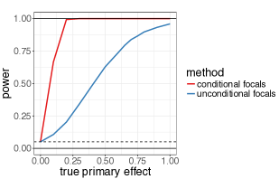
Figure 1: Power of the test of no primary effect obtained with choice of focals unconditional to the observed assignment (Athey et al. (2017)) versus conditional choice, for different true values of the true primary effect.

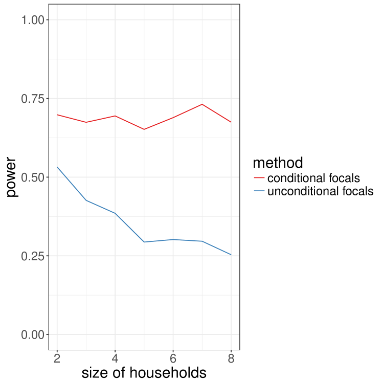
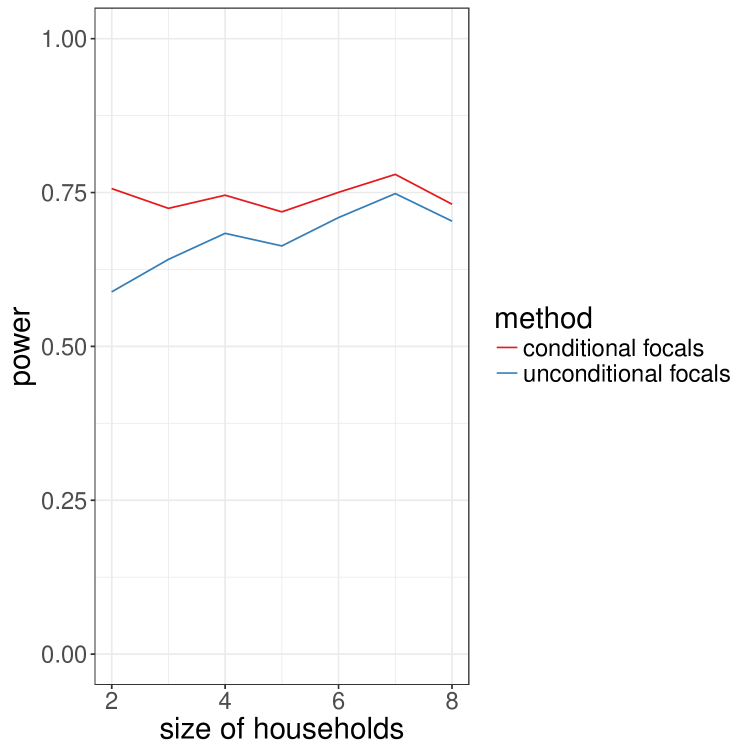
Figure 2: Power of the two methods for testing the null hypotheses of no primary effect, on the left, and no spillover effect, on the right, as a function of household size $n_{i}$.

C.2 Details of analysis: covariate adjustment

In all the analyses in the paper, covariates where taken into account via the same model-assisted approach used in Section 7 and Section 9.2 of Basse and Feller (2017). Briefly, we use a holdout set to estimate the parameter of a regression, then we use those estimators parameters to obtain predicted values $\{\hat{Y}_{i}\}_{i}$ for the outcomes in our sample and compute the residuals $\hat{e}_{i}=Y_{i}^{\mathrm{obs}}-\hat{Y}_{i}$. We then apply the conditional testing methodology to the residuals, instead of the original potential outcomes; in that way, the residuals can be thought of as transformed outcomes. Note that this approach is similar to that used by Rosenbaum (2002).

C.3 Details of analysis: confidence intervals

We ran an additional analysis comparing the size of confidence intervals for our method and for that of Athey et al. (2017). Specifically, for each of $H_{0}^{s}$ and $H_{0}^{p}$, we drew 100 focal sets using our method, and 100 using the method of Athey et al. (2017), and computed the associated confidence intervals, obtained by inverting sequences of Fisher randomization tests (Rosenbaum, 2002). Figure 3 summarizes the results. We see that our method leads to smaller confidence intervals compared to the method of Athey et al. (2017), and that the difference is larger for the primary effect than for the spillover effect.

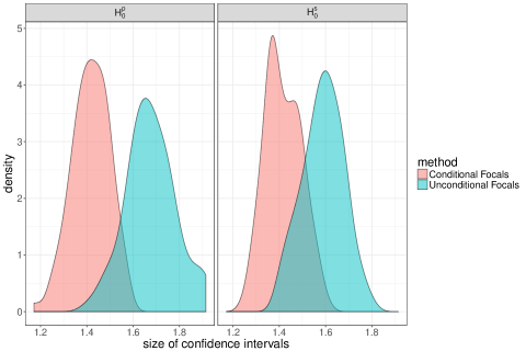
Figure 3: Size of the confidence intervals for the primary and spillover effects obtained by the two methods.

C.4 Details of analysis: point estimates

Point estimates are obtained using a variant of the Hodges-Lehmann estimator (Hodges Jr and Lehmann, 1963). Specifically, for a conditioning event $\mathcal{C}$, we numerically solve the equation $E(T\mid\mathcal{C},H^{P}_{\tau})=T^{\mathrm{obs}}$, where $H^{P}_{\tau}$ is the null hypothesis $Y_{i}(1,1)=Y_{i}(0,0)$, by considering a grid of values for $\tau$, and computing the expectation of the null distribution of $T$ under the hypothesis $H^{P}_{\tau}$ and keeping the value $\hat{\tau}$ of $\tau$ that is closest to $T^{\mathrm{obs}}$.

C.5 Details of analysis: results for testing $H_{0}^{P}$

The median value of the Hodges-Lehmann for the primary effect is approximately equal for both choices of functions $f$ and is approximately equal to $-1.5$ days, with associated confidence interval $[-2.2,0.75]$ for our method, and $[-2.3,-0.8]$ for the method of Athey et al. (2017). The average length of confidence intervals obtained with our method is $1.4$ days, versus $1.6$ days for the method of Athey et al. (2017). The fraction of focals leading to a p-value below $0.05$ is $100\%$ in our case, based on a Monte-Carlo estimate from 100 replications, versus $92\%$ for the method in Athey et al. (2017).

Appendix D Comparison of powers of tests

D.1 Model, p-values and power

In this section, we make an approximate theoretical analysis of the power of our test and the power of the test by Athey et al. (2017). Our analysis is performed under two approximations. First, in the context of classical Fisher randomization tests, we argue that, in general, tests that are balanced and use more units are more powerful. So, balance and size of treatment arms can be used as a proxy for the power of the test. Second, we argue that since in the two-stage randomization case, our test and the test in Athey et al. (2017) can be conceived as classical Fisher randomization tests run on the focal units, the aforementioned power approximation for the classical Fisher randomization test applies.

Consider a classical Fisher randomization test, with complete randomization where $N_{1}$ out of $N$ units are treated. Let $p=N_{1}/N$. Suppose that that the true effect is constant additive $\tau$, and that we test for the null of no effect $H_{0}$. In order to give concrete analytical heuristics, we consider a model for the potential outcomes and focus on asymptotics; see also Lehmann and Romano (2006) for this approach:

$$Y_{i}(Z_{i})\sim\tau Z_{i}+\mathcal{N}(\mu,\sigma^{2}).$$

As mentioned, we will focus our argument on asymptotic heuristics. Denote by $V=var(T\mid Y^{\mathrm{obs}},H_{0})$ the randomization variance of the test statistics conditional on $Y^{\mathrm{obs}}$, and assuming $H_{0}$ is true. We have, for large $N$:

$$V=\frac{1}{N}\bigg{[}\frac{\sigma^{2}}{p(1-p)}+\tau^{2}\bigg{]}.$$

Denote by $V^{\mathrm{obs}}$ the variance of the test statistic $V^{\mathrm{obs}}=var(T)$. We have, for large $N$,

$$V^{\mathrm{obs}}=V-\frac{\tau^{2}}{N},$$

and so by applying the appropriate CLT’s, we have:

$$\frac{T}{V^{1/2}}\approx\mathcal{N}(0,1),\qquad\frac{T^{\mathrm{obs}}-\tau}{(V^{\mathrm{obs}})^{1/2}}\approx\mathcal{N}(0,1).$$

Note the application of the CLT is heuristic here, and some regularity conditions are required. We can then obtain an approximation of the distribution of a one-sided p-value for large N:

$$\mathrm{pval} ={\rm pr}(T\geq T^{\mathrm{obs}})$$

$$\approx 1-\Phi\bigg{(}\frac{T^{\mathrm{obs}}}{V^{1/2}}\bigg{)},$$

using the asymptotics from above. We can then verify that:

$$\frac{T^{\mathrm{obs}}}{V^{1/2}}=\frac{T^{\mathrm{obs}}-\tau}{(V^{\mathrm{obs}})^{1/2}}(1-C)^{1/2}+(NC)^{1/2}$$

$$\approx W(1-C)^{1/2}+(NC)^{1/2},$$

where $W\sim\mathcal{N}(0,1)$ and $C=\tau^{2}[\sigma^{2}/\{p(1-p)\}+\tau^{2}]^{-1}$ and so :

$$\mathrm{pval}=1-\Phi(W(1-C)^{1/2}+(NC)^{1/2}).$$ (28)

We can use the approximation of Equation (28) to deal with the power. For $\alpha\in[0,1]$, the power of the test at level $\alpha$ will be

$$\beta_{\alpha}={\rm pr}(\mathrm{pval}\leq\alpha),$$

but we verify that

$$\mathrm{pval}\leq\alpha\quad\Leftrightarrow\quad W\geq\frac{\Phi^{-1}(1-\alpha),-(NC)^{1/2}}{(1-C)^{1/2}}$$

and so the power of the test will be approximately:

$$\beta_{\alpha}=1-\Phi\bigg{(}\frac{\Phi^{-1}(1-\alpha)-(NC)^{1/2}}{(1-C)^{1/2}}\bigg{)}.$$ (29)

D.2 Comparing classical tests

We are interested in comparing tests with different proportions $p$ of treated units, and with different numbers $N$ of units. We will denote these quantities by $N^{(1)}$ and $N^{(2)}$ for the number of units, and $p^{(1)}$ and $p^{(2)}$ for the proportions. Let $\beta^{(1)}$ and $\beta^{(2)}$ be the associated powers. Finally, notice that:

$$\beta^{(1)}\leq\beta^{(2)} \Leftrightarrow\frac{\Phi^{-1}(1-\alpha)-(N^{(1)}C^{(1)})^{1/2}}{(1-C^{(1)})^{1/2}}\geq\frac{\Phi^{-1}(1-\alpha)-(N^{(2)}C^{(2)})^{1/2}}{(1-C^{(2)})^{1/2}}$$

$$\Leftrightarrow\gamma^{(1)}\geq\gamma^{(2)}$$

where $\gamma^{(1)}=\{\Phi^{-1}(1-\alpha)-(N^{(1)}C^{(1)})^{1/2}\}/\{(1-C^{(1)})^{1/2}\}$

Suppose that both tests have the same number of units $N^{(1)}=N^{(2)}=N$, but different fractions of treated units $p^{(1)}\neq p^{(2)}$. We have

$$\gamma^{(1)}-\gamma^{(2)} =N^{1/2}\bigg{(}\frac{(C^{(2)})^{1/2}}{1-(C^{(2)})^{1/2}}-\frac{(C^{(1)})^{1/2}}{1-(C^{(1)})^{1/2}}\bigg{)}+\bigg{(}\frac{\Phi^{-1}(1-\alpha)}{(1-C^{(1)})^{1/2}}-\frac{\Phi^{-1}(1-\alpha)}{(1-C^{(2)})^{1/2}}\bigg{)}$$

$$\rightarrow N^{1/2}\bigg{(}\frac{(C^{(2)})^{1/2}}{1-(C^{(2)})^{1/2}}-\frac{(C^{(1)})^{1/2}}{1-(C^{(1)})^{1/2}}\bigg{)}$$

and so for large $N$,

$$\gamma^{(1)}-\gamma^{(2)}\geq 0 \Leftrightarrow\frac{(C^{(2)})^{1/2}}{1-(C^{(2)})^{1/2}}-\frac{(C^{(1)})^{1/2}}{1-(C^{(1)})^{1/2}}\geq 0$$

$$\Leftrightarrow p^{(1)}(1-p^{(1)})\leq p^{(2)}(1-p^{(2)})$$

$$\Leftrightarrow|p^{(1)}-\frac{1}{2}|\geq|p^{(2)}-\frac{1}{2}|.$$

So in conclusion:

$$\beta^{(1)}\leq\beta^{(2)}\quad\Leftrightarrow\quad|p^{(1)}-\frac{1}{2}|\geq|p^{(2)}-\frac{1}{2}|$$

which, in words, means that the balanced test has more power asymptotically.

Suppose that $N^{(1)}\neq N^{(2)}$ but that the fractions of treated units in each test is identical. That is, $p^{(1)}=p^{(2)}=p$. The immediate consequence is that $C^{(1)}=C^{(2)}=C$, and so:

$$\gamma^{(1)}-\gamma^{(2)}=\frac{C^{1/2}}{1-C^{1/2}}\bigg{(}(N^{(2)})^{1/2}-(N^{(1)})^{1/2}\bigg{)},$$

and so:

$$\beta^{(1)}\leq\beta^{(2)}\quad\Leftrightarrow N^{(1)}\leq N^{(2)},$$

which in words means that the test with more units has more power asymptotically.

D.3 Comparing our test with test of Athey et al. (2017)

If we restrict our attention to the special case where all households have equal size $n_{i}=n$, then both our method and the method of Athey et al. (2017) can be seen as classical Fisher randomization tests applied on a set of ”effective” focal units, where the set of ”effective focals” is always at least as large with our method as in the method of Athey et al. (2017), and is always balanced if the initial assignment ${\rm pr}(Z)$ is balanced. We can then leverage the result of Section D.2 to argue heuristically that for classical Fisher randomization tests, larger and more balanced is generally better, and so we expect our method to lead to more powerful test. This has been confirmed in the simulations of Section C.1 and in the analysis.

D.4 Comparison with unconditional focal selection under a different design

In this section, we perform an analysis outside of the two-stage design setting to illustrate the generality of our framework. We assume there is a network between units such that $\mathcal{N}_{i}$ denotes the neighborhood of unit $i$. As in the two-stage setting, we will show that being able to condition on the observed treatment assignment, which is possible in our framework, can lead to better randomization tests.

We consider a network between units and the following exposure functions:

$$h_{i}(Z)=\begin{cases}a&\text{ if }\quad Z_{i}=1,\\ b&\text{ if }\quad Z_{i}=0,\,\,\sum_{j\in\mathcal{N}_{i}}Z_{j}<d,\\ c&\text{ if }\quad Z_{i}=0,\,\,\sum_{j\in\mathcal{N}_{i}}Z_{j}>d,\\ \end{cases}$$

and assume that $N_{1}$ units are treated completely at random in the network, and that we wish to test the null hypothesis:

$$H_{0}:Y_{i}(Z)=Y_{i}(Z^{\prime}),i=1,\ldots,N,\,\,\,\text{ for all }Z,Z^{\prime}:h_{i}(Z),h_{i}(Z^{\prime})\in\{b,c\}.$$

This example is very different from the two-stage randomization setting considered in the main text, but there is one commonality: the units who received treatment are useless for testing $H_{0}$, and so it is wasteful to include them in the focal set. It is easy to verify that if focals are chosen completely at random, the distribution of the effective number of focals is $|\textsc{eff}(\mathcal{U})|\sim M-\text{Hypergeom}(N,N_{1},M)$, and so the expected number of focal units is $E\{|\textsc{eff}(\mathcal{U})|\}=M-M(N_{1}/N)$. In the case where half the units are treated, that is $N_{1}=N/2$, we have:

$$E\{|\textsc{eff}(\mathcal{U})|\}=\frac{M}{2},$$

so in effect we lose half of the focal units. Choosing focals unconditionally but based on $\epsilon$-nets would be better than choosing the focals completely at random but would not solve the fundamental reason why power is lost. Moreover, if choosing focals based on $\epsilon$-nets is helpful, then it could always be combined with conditioning on the observed assignment to yield an even more powerful test.

To illustrate our framework in this setting, we could use following procedure:

1. Draw $Z$, completely at random with $N_{1}$ treated units, and $N_{0}$ control units.

2. Choose $M$ focal units at random among the $N_{0}$ units with $Z_{i}=0$. Let $\mathcal{U}$ be the set of focal units.

3. Draw $Z^{\prime}\sim{\rm pr}(Z^{\prime}\mid\mathcal{U})$ as follows. Set $Z^{\prime}_{i}=0$ for all $i\in\mathcal{U}$. Then choose $N_{0}-M$ units at random among the $N-M$ non-focal units, and set $Z^{\prime}_{i}=0$ for these units. Finally, set $Z_{i}=1$ for the remaining $N_{1}$ units.

We claim that the abovementioned procedure in Step 3 samples indeed from the correct conditional randomization distribution.

Proof.

By definition of the procedure in Steps 2 and 3, it holds that ${\rm pr}(Z^{\prime})\propto 1$ if $\sum_{i}Z_{i}^{\prime}=N_{1}$, and also ${\rm pr}(\mathcal{U}\mid Z^{\prime})=$ const., if $|\mathcal{U}|=M$ and $Z^{\prime}_{i}=0$ for every $i\in\mathcal{U}$. Therefore, ${\rm pr}(Z^{\prime}\mid\mathcal{U})=\text{Unif}(\mathcal{Z}(\mathcal{U}))$, where $\mathcal{Z}(\mathcal{U})=\{Z:\text{for all }i\in\mathcal{U},Z_{i}=0\,\,\text{ and }\,\,\sum_{i}Z_{i}=N_{1}\}$. Which is what step 3 does. ∎

Note that in this case our approach does not lead to a permutation test; and neither does the method of Athey et al. Nevertheless, it leads to a procedure that is easily implementable and that uses more information than that of Athey et al.

Appendix E Testing the null hypothesis of no primary effect

The paper focused on testing the null hypothesis of no spillover effects $H_{0}^{S}$. In this section, we briefly give equivalent results for testing the null hypothesis of no primary effect $H_{0}^{P}$. We omit the proofs, since they follow exactly the same outlines as the proof for $H_{0}^{S}$. A simple choice of $f$ function for testing the null hypothesis of no primary effect is

$$f(\mathcal{U}\mid Z)=\text{Unif}\{\mathbb{U}^{(P)}(Z)\},$$

where

$$\mathbb{U}^{(P)}(Z)=\{\mathcal{U}\in\mathbb{U}:Z_{i}=1\Rightarrow i\in\mathcal{U},\,\,\,\text{for all }i\in\mathcal{U}\quad\text{ and }\quad\sum_{i}\mathbb{I}(i\in\mathcal{U})R_{ij}=1,\text{for every household }j\}.$$

If applied to Theorem 2, this choice of $f$ leads to the following procedure, which mirrors that of Proposition 1:

1. In control households, $W_{j}=0$, choose one unit at random. In treated households, $W_{j}=1$, choose the treated unit as focal.

2. Compute the distribution of the test statistic Equation (20) induced by all permutations of exposures on focal units, using $a=(0,0)$ and $b=(1,1)$ as the contrasted exposures.

3. Compute the p-value.

This procedure is valid conditionally and marginally for testing $H_{0}^{P}$.

Appendix F Notes on the choice of exposure mapping $h()$

F.1 More complex exposure mappings

The class of null hypotheses that our method is designed to test is summarized in Equation (7) of our manuscript, reproduced below for convenience:

$$H_{0}:Y_{i}(Z)=Y_{i}(Z^{\prime}),(i=1,\ldots,N)\,\,\text{for all}\,\,Z,Z^{\prime}\text{ for which }h_{i}(Z),h_{i}(Z^{\prime})\in\{a,b\},$$ (30)

for some exposure function $h$, the choice of which is limited by a few theoretical and practical considerations. The only strong theoretical constraint implicit in Equation (7) of the manuscript is that the two exposures $a$ and $b$ being contrasted must be well defined for all units under consideration. For instance, in the test of no spillovers $H_{0}^{s}$, the two exposures contrasted are the spillover exposure $(1,0)$, and the control exposure $(0,0)$, which are well defined for all units. If we had households with a single individual, then the exposure $(1,0)$ would not be defined for that unit and the null hypothesis of Equation (7) would consequently be ill-posed if it included that unit.

Still, the formulation in Equation (30) provides enough flexibility to test a wide variety of null hypotheses. Here, we illustrate with a couple of short but representative examples on network interference. Similar to Athey et al. (2017), let $G_{ij}=1$ if units $i$ and $j$ are neighbors in the network, and $G_{ij}=0$ otherwise. By convention, $G_{ii}=0$ for all $i$.

Suppose we want to test spillovers on control units from first-order neighbors. Then, we could define:

$$h_{i}(Z)=\begin{cases}a&\text{if $Z_{i}=1$},\\ b&\text{if $Z_{i}=0$, \, $\sum_{j}G_{ij}Z_{j}>0$},\\ c&\text{if $Z_{i}=0$, \, $\sum_{j}G_{ij}Z_{j}=0$}.\end{cases}$$

Now testing the hypothesis in Equation (30) contrasting the exposures $b$ and $c$ defined above will test whether there are spillovers on control units.

As another example, suppose we want to test spillovers on control units from up to second-order neighbors. Let $H_{ij}=1$ if $i$ and $j$ are second-order neighbors but not first-order neighbors, so $G_{ij}=0$. Then, we could define:

$$h_{i}(Z)=\begin{cases}a&\text{if $Z_{i}=1$},\\ b&\text{if $Z_{i}=0$, \, $\sum_{j}(G_{ij}+H_{ij})Z_{j}>0$},\\ c&\text{if $Z_{i}=0$, \, $\sum_{j}(G_{ij}+H_{ij})Z_{j}=0$}.\end{cases}$$

Now testing the hypothesis in Equation (30) contrasting the exposures $b$ and $c$ defined above will test whether there are spillovers on control units from first-order or second-order neighbors. We could also test the hypothesis that there are no second-order spillovers without putting constraints on first-order spillovers. For that test, we could define:

$$h_{i}(Z)=\begin{cases}a&\text{if $Z_{i}=1$},\\ b&\text{if $Z_{i}=0$, \, $\sum_{j}G_{ij}Z_{j}>0$},\\ c&\text{if $Z_{i}=0$, \, $\sum_{j}G_{ij}Z_{j}=0$, \, $\sum_{j}H_{ij}Z_{j}>0$},\\ d&\text{if $Z_{i}=0$, \, $\sum_{j}(G_{ij}+H_{ij})Z_{j}=0$}.\end{cases}$$

Now testing the hypothesis in Equation (30) contrasting the exposures $c$ and $d$ defined above will test whether there are spillovers on control units from second-order neighbors only. We can follow similar approaches for testing higher than second-order spillovers.

We now consider an example closer to the scenario of our application. Consider the same design as in our manuscript, but assume that all households have $n=3$ units. We are interested in testing whether an untreated unit in a treated household receives a different spillover if the eldest of its two siblings is treated compared to the spillover received if the youngest of its two siblings is treated.

In order to test this null hypothesis, we need to consider a more complex exposure mapping than the one in our manuscript. Let $E_{i}\in\{0,1\}$ be the treatment assignment of the eldest of unit $i$’s two siblings, and consider the exposure mapping:

$$h_{i}(Z)=(H_{i},Z_{i},E_{i}).$$

Each unit now has four potential outcomes:

$$Y_{i}(Z)\in\{Y_{i}(1,1,0),Y_{i}(0,0,0),Y_{i}(1,0,1),Y_{i}(1,0,0)\},$$

the other combinations being impossible. With this exposure mapping the null hypothesis of no differential spillover effect from the eldest sibling can be written as:

$$H_{0}:Y_{i}(1,0,1)=Y_{i}(1,0,0)\,\,(i=1,\ldots,N).$$

F.2 Exposure mappings and the choice of test statistic

The choice of test statistic $T$ is related to the choice of exposure mapping $h$ to the extent that it provides a good estimate of the differential effect between exposures $a$ and $b$ in Equation (30). Furthermore, if we have some prior belief about the potential outcomes and the interference structure, it can be incorporated in the test statistic. Athey et al. (2017) have a nice and insightful discussion about possible test statistics in Section 5.3 of their paper, which is applicable in our setting as well.

References

- Aronow (2012) Aronow, P. M. (2012). A general method for detecting interference between units in randomized experiments. Sociological Methods & Research 41(1), 3–16.
- Aronow and Samii (2017) Aronow, P. M. and C. Samii (2017). Estimating average causal effects under general interference, with application to a social network experiment. The Annals of Applied Statistics 11(4), 1912–1947.
- Athey et al. (2017) Athey, S., D. Eckles, and G. W. Imbens (2017). Exact p-values for network interference. Journal of the American Statistical Association (just-accepted), Forthcoming.
- Basse and Feller (2017) Basse, G. and A. Feller (2017). Analyzing two-stage experiments in the presence of interference. Journal of the American Statistical Association (just-accepted), Forthcoming.
- Bowers et al. (2013) Bowers, J., M. M. Fredrickson, and C. Panagopoulos (2013). Reasoning about interference between units: A general framework. Political Analysis 21(1), 97–124.
- Cox (1958) Cox, D. R. (1958). Planning of Experiments. New York: John Wiley & Sons.
- Fisher (1935) Fisher, R. A. (1935). The Design of Experiments. Edinburgh: Oliver & Boyd.
- Geyer and Meeden (2005) Geyer, C. J. and G. D. Meeden (2005). Fuzzy and randomized confidence intervals and p-values. Statistical Science 20(4), 358–366.
- Hennessy et al. (2016) Hennessy, J., T. Dasgupta, L. Miratrix, C. Pattanayak, and P. Sarkar (2016). A conditional randomization test to account for covariate imbalance in randomized experiments. Journal of Causal Inference 4(1), 61–80.
- Hodges Jr and Lehmann (1963) Hodges Jr, J. L. and E. L. Lehmann (1963). Estimates of location based on rank tests. The Annals of Mathematical Statistics, 598–611.
- Hudgens and Halloran (2008) Hudgens, M. G. and M. E. Halloran (2008). Toward causal inference with interference. Journal of the American Statistical Association 103(482), 832–842.
- Lehmann and Romano (2006) Lehmann, E. L. and J. P. Romano (2006). Testing statistical hypotheses. Springer Science & Business Media.
- Manski (2013) Manski, C. F. (2013). Identification of treatment response with social interactions. The Econometrics Journal 16(1), S1–S23.
- Rigdon and Hudgens (2015) Rigdon, J. and M. G. Hudgens (2015). Exact confidence intervals in the presence of interference. Statistics & Probability Letters 105, 130–135.
- Rogers and Feller (2018) Rogers, T. and A. Feller (2018). Reducing student absences at scale by targeting parents’ misbeliefs. Nature Human Behavior 2, 335–342.
- Rosenbaum (2002) Rosenbaum, P. R. (2002). Covariance adjustment in randomized experiments and observational studies. Statistical Science 17(3), 286–327.
- Rubin (1980) Rubin, D. B. (1980). Comment. Journal of the American Statistical Association 75(371), 591–593.
- Sobel (2006) Sobel, M. E. (2006). What do randomized studies of housing mobility demonstrate? Causal inference in the face of interference. Journal of the American Statistical Association 101(476), 1398–1407.
- Toulis and Kao (2013) Toulis, P. and E. Kao (2013). Estimation of causal peer influence effects. Journal of Machine Learning Research 28(3), 1489–1497.