Scalar, Vector and Tensor Harmonics on the Three-Sphere

Abstract

Scalar, vector and tensor harmonics on the three-sphere were introduced originally to facilitate the study of various problems in gravitational physics. These harmonics are defined as eigenfunctions of the covariant Laplace operator which satisfy certain divergence and trace identities, and ortho-normality conditions. This paper provides a summary of these properties, along with a new notation that simplifies and clarifies some of the key expressions. Practical methods are described for accurately and efficiently computing these harmonics numerically, and test results are given that illustrate how well the analytical identities are satisfied by the harmonics computed numerically in this way.

1 Introduction

Scalar, vector and tensor harmonics have been introduced as part of investigations of a variety of gravitational physics problems in spaces with the topology of the three-sphere, $\mathbb{S}^{3}$. These include studies of the dynamics of nearly homogeneous and isotropic cosmological models Lifshitz1963 ; Halliwell1985 ; Lindblom2013 , the properties of quantum field theories in these spaces Adler1973 ; Adler1977 , and the dynamics of homogeneous collapsing stellar models Gerlach1978 . In addition to these application-oriented studies, a number of more mathematically focused investigations of the properties of these harmonics have been reported in the literature. These include the analysis of these harmonics as eigenfunctions of the covariant Laplace operator on $\mathbb{S}^{3}$ Sandberg1978 ; Rubin1984 ; Rubin1985 ; LachiezeRey2005 ; BenAchour2016 , and as representations of the Lie groups $SU(2)$ Jantzen1978 and $SO(4,1)$ Higuchi1991 .

Our intent here is to provide a concise summary of some of the most useful properties of these harmonics, along with practical methods for evaluating them numerically. Various incompatible notations for these harmonics have been introduced and used in the references cited above. We attempt to simplify and clarify this situation by introducing a new uniform notation for the scalar, vector and tensor harmonics that is analogous to notation commonly used for the more familiar harmonics on the two-sphere, $\mathbb{S}^{2}$. We summarize the useful analytical identities satisfied by these harmonics, including their covariant Laplace operator eigenvalue equations, their trace and divergence identities, and their integral ortho-normality properties. Although we have independently verified all of these identities analytically, we do not attempt to derive or present the proofs of them here. These properties have all been derived previously in the works cited above. We do, however, present straightforward methods for evaluating these harmonics numerically, and we present numerical tests that demonstrate accuracy and convergence for our implementation of these numerical methods. These tests illustrate how well the various harmonic identities are satisfied as functions of the numerical resolution used to evaluate them, and also as functions of the order and the tensor rank of the harmonics. Section 2 summarizes the properties of the scalar harmonics, Sec. 3 summarizes the vector and anti-symmetric second-rank tensor harmonics, Sec. 4 summarizes the symmetric second-rank tensor harmonics, and finally Sec. 5 describes the results of our numerical tests that evaluate and illustrate the accuracy of our numerical methods.

2 Scalar Harmonics

We use the notation $Y^{k\ell m}$ to denote the scalar harmonics on $\mathbb{S}^{3}$. The integers $k$, $\ell$, and $m$ with $k\geq\ell\geq 0$ and $\ell\geq m\geq-\ell$ indicate the order of the harmonic. These harmonics are eigenfunctions of the covariant Laplace operator:

$$\nabla^{a}\nabla_{a}Y^{k\ell m}=-\frac{k(k+2)}{R_{3}^{2}}Y^{k\ell m},$$ (1)

where $R_{3}$ is the radius, and $\nabla_{a}$ is the covariant derivative associated with the round metric on $\mathbb{S}^{3}$. It is often useful to express this metric in terms of spherical coordinates $x^{a}=(\chi,\theta,\varphi)$:

$$ds^{2} = g_{ab}dx^{a}dx^{b},$$ (2)

$$= R_{3}^{2}\left[d\chi^{2}+\sin^{2}\chi\left(d\theta^{2}+\sin^{2}\theta\,d\varphi^{2}\right)\right].$$

The $\mathbb{S}^{3}$ scalar harmonics can be expressed in terms of the standard $\mathbb{S}^{2}$ scalar harmonics $Y^{\ell m}$ by defining the functions $H^{k\ell}(\chi)$:

$$Y^{k\ell m}(\chi,\theta,\varphi)=H^{k\ell}(\chi)Y^{\ell m}(\theta,\varphi).$$ (3)

The $H^{k\ell}(\chi)$ are determined by inserting Eq. (3) into Eq. (1), to obtain the following ordinary differential equation:

$$0 = \frac{d^{2}H^{k\ell}}{d\chi^{2}}+2\cot\chi\frac{dH^{k\ell}}{d\chi}+\left[k(k+2)-\ell(\ell+1)\csc^{2}\chi\right]H^{k\ell}.\qquad$$ (4)

This differential equation can be solved most conveniently by introducing $C^{k\ell}(\chi)$ such that

$$H^{k\ell}(\chi)=\sin^{\ell}\!\chi\,C^{k\ell}(\chi).$$ (5)

These $C^{k\ell}$ (which are proportional to the Gegenbauer polynomials) are given, for $k=\ell$ and $k=\ell+1$, by the expressions

$$C^{\ell\ell} = (-1)^{\ell+1}2^{\ell}\ell\kern 1.00006pt!\,\sqrt{\frac{2(\ell+1)}{\pi(2\ell+1)!}},\qquad$$ (6)

$$C^{\ell+1\,\ell} = \sqrt{2(\ell+2)}\cos\chi\,C^{\ell\ell}.$$ (7)

The solutions for $k>\ell+1$ are determined by applying the recursion relation

$$\!\!\!\!\!\!\!\!C^{k+2\,\ell}=2\cos\chi\sqrt{\frac{(k+3)(k+2)}{(k+3+\ell)(k+2-\ell)}}\,C^{k+1\,\ell}\qquad$$

$$\qquad\qquad\quad-\sqrt{\frac{(k+3)(k+2+\ell)(k+1-\ell)}{(k+1)(k+3+\ell)(k+2-\ell)}}\,C^{k\ell},\qquad$$ (8)

iteratively starting with the $k=\ell$ and $k=\ell+1$ solutions given above. This allows the $Y^{k\ell m}$ to be determined numerically in a straightforward way as functions of the spherical coordinates $(\chi,\theta,\varphi)$ using Eqs. (3) and (5)–(8).

The $\mathbb{S}^{3}$ scalar harmonics $Y^{k\ell m}$, defined and normalized as above, satisfy the following ortho-normality conditions:

$$\delta^{\,kk^{\prime}}\delta^{\,\ell\ell^{\prime}}\delta^{\,mm^{\prime}}=\frac{1}{R_{3}^{3}}\int Y^{k\ell m}\,Y^{*k^{\prime}\ell^{\prime}m^{\prime}}\sqrt{g}\,d^{\,3}x.$$ (9)

Any scalar function $S$ on the three-sphere can be written as an expansion in terms of these scalar harmonics:

$$S=\sum_{k=0}^{\infty}\sum_{\ell=0}^{k}\sum_{m=-\ell}^{\ell}S^{k\ell m}\,Y^{k\ell m}.$$ (10)

The ortho-normality relations in Eq. (9) imply the following integral expressions for the expansion coefficients $S^{k\ell m}$,

$$S^{k\ell m}=\frac{1}{R_{3}^{3}}\int S\,Y^{*k\ell m}\sqrt{g}\,d^{\,3}x.$$ (11)

We find it useful in our numerical work on the three-sphere to represent fields in coordinates other than the standard spherical coordinate system. Let the transformation law $x^{b}=x^{b}(\bar{x}^{a})$, denote the transformation between spherical coordinates $x^{a}=(\chi,\theta,\varphi)$ and some other useful coordinates $\bar{x}^{a}$. Given these coordinate transformation laws, it is straightforward to determine $Y^{k\ell m}(\bar{x}^{a})$ simply by composing the standard spherical coordinate representation described above, $Y^{k\ell m}(x^{b})$, with the coordinate transformation law $x^{b}(\bar{x}^{a})$ to obtain $Y^{k\ell m}(\bar{x}^{b})=Y^{k\ell m}[x^{a}(\bar{x}^{b})]$.

3 Vector Harmonics

The vector harmonics on $\mathbb{S}^{3}$ are completely determined by the scalar harmonics $Y^{k\ell m}$ and their derivatives. In particular the three classes of vector harmonics, which we denote $Y^{k\ell m}_{(A\,)a}$ for ${\scriptstyle A}=0,1,2$, are defined by

$$Y^{k\ell m}_{(0)\,a} = \frac{R_{3}}{\sqrt{k(k+2)}}\nabla_{a}Y^{k\ell m},$$ (12)

$$Y^{k\ell m}_{(1)\,a} = \frac{R_{3}^{2}}{\sqrt{\ell(\ell+1)}}\epsilon_{a}{}^{bc}\nabla_{b}Y^{k\ell m}\nabla_{c}\cos\chi,$$ (13)

$$Y^{k\ell m}_{(2)\,a} = \frac{R_{3}}{k+1}\epsilon_{a}{}^{bc}\nabla_{b}Y^{k\ell m}_{(1)\,c},$$ (14)

where $\epsilon_{abc}$ is the totally antisymmetric tensor volume element, which satisfies $\nabla_{d}\epsilon_{abc}=0$. All the vector harmonics vanish identically for $k=0$, and the harmonics $Y^{k\ell m}_{(1)\,a}$ and $Y^{k\ell m}_{(2)\,a}$ are not well defined for $\ell=0$. Thus the vector harmonics are defined only for $k\geq k^{V(A)}_{\mathrm{min}}$ and $\ell\geq\ell^{V(A)}_{\mathrm{min}}$, where the values of $k^{V(A)}_{\mathrm{min}}$ and $\ell^{V(A)}_{\mathrm{min}}$ are given in Table 1.

$\scriptstyle A$	$k_{\mathrm{min}}^{V(A)}$	$\ell_{\mathrm{min}}^{V(A)}$	$k_{\mathrm{min}}^{T(A)}$	$\ell_{\mathrm{min}}^{T(A)}$
0	1	0	0	0
1	1	1	2	1
2	1	1	2	1
3	-	-	2	0
4	-	-	2	2
5	-	-	2	2

Table 1: Minimum values of the harmonic order parameters $k\geq k_{\mathrm{min}}$ and $\ell\geq\ell_{\mathrm{min}}$ for the various classes of vector and tensor harmonics.

The vector harmonics $Y^{k\ell m}_{(A)\,a}$ are eigenfunctions of the covariant Laplace operator on $\mathbb{S}^{3}$, which satisfy the following eigenvalue equations,

$$\nabla^{b}\nabla_{b}Y^{k\ell m}_{(0)\,a} = \frac{2-k(k+2)}{R_{3}^{2}}Y^{k\ell m}_{(0)\,a},$$ (15)

$$\nabla^{b}\nabla_{b}Y^{k\ell m}_{(1)\,a} = \frac{1-k(k+2)}{R_{3}^{2}}Y^{k\ell m}_{(1)\,a},$$ (16)

$$\nabla^{b}\nabla_{b}Y^{k\ell m}_{(2)\,a} = \frac{1-k(k+2)}{R_{3}^{2}}Y^{k\ell m}_{(2)\,a}.$$ (17)

These vector harmonics also satisfy the following divergence identities,

$$\nabla^{a}Y^{k\ell m}_{(0)\,a} = -\frac{\sqrt{k(k+2)}}{R_{3}}Y^{k\ell m},$$ (18)

$$\nabla^{a}Y^{k\ell m}_{(1)\,a} = 0,$$ (19)

$$\nabla^{a}Y^{k\ell m}_{(2)\,a} = 0.$$ (20)

The vector harmonics defined in Eqs. (12)–(14) have been normalized so they satisfy the following ortho-normality relations,

$$\delta_{(A)(B)}\delta^{\,kk^{\prime}}\delta^{\,\ell\ell^{\prime}}\delta^{\,mm^{\prime}}=\frac{1}{R_{3}^{3}}\int\!\!g^{ab}\,Y^{\,k\ell m}_{(A)\,a}\,Y^{\,*k^{\prime}\ell^{\prime}m^{\prime}}_{(B)\,b}\!\sqrt{g}\,d^{\,3}x,\!\!\!\!\!$$

(21)

for $k,k^{\prime}\geq k^{V(A)}_{\mathrm{min}}$ and $\ell,\ell^{\prime}\geq\ell^{V(A)}_{\mathrm{min}}$. It is often useful and convenient to express vector fields $V^{a}$ as expansions in terms of these vector harmonics:

$$V^{a}=g^{ab}\sum_{A=0}^{2}\sum_{k=k^{V(A)}_{\mathrm{min}}}^{\infty}\sum_{\ell=\ell^{V(A)}_{\mathrm{min}}}^{k}\sum_{m=-\ell}^{\ell}V^{k\ell m}_{(A)}\,Y^{k\ell m}_{(A)\,b}.\qquad$$ (22)

The ortho-normality relations, Eq. (21), imply that the expansion coefficients $V^{k\ell m}_{(A)}$ are simply the integral projections of the vector field onto the corresponding vector harmonics:

$$V^{k\ell m}_{(A)}=\frac{1}{R_{3}^{3}}\int V^{a}\,Y^{*k\ell m}_{(A)\,a}\sqrt{g}\,d^{\,3}x.$$ (23)

We point out that the new notation we have introduced here for these harmonics makes it much simpler to express the ideas contained in Eqs. (21)–(23) than it would have been using previous notations.

The expressions for the vector harmonics given in Eqs. (12)–(14) are covariant, so it is straightforward to evaluate them in any convenient coordinates. To evaluate them numerically, we start by computing the scalar harmonics $Y^{k\ell m}$ numerically on a grid of points in the chosen coordinates using the methods described in Sec. 2. The gradients of the scalar harmonics are then evaluated on this grid using any convenient numerical method (e.g, finite difference or pseudo-spectral). Finally these gradients are combined algebraically using the expressions in Eqs. (12)–(14) to determine the vector harmonics on that grid of points.

Anti-symmetric tensor fields, $W_{ab}=-W_{ba}$, in three-dimensions are dual to vector fields: for every $W_{ab}$ there exists a vector field $V^{a}$ such that $W_{ab}=\epsilon_{abc}V^{c}$. Thus arbitrary anti-symmetric tensor fields on $\mathbb{S}^{3}$ can be expressed in terms of the vector harmonics:

$$W_{ab}=\epsilon_{ab}{}^{c}\sum_{A=0}^{2}\sum_{k=k^{V(A)}_{\mathrm{min}}}^{\infty}\sum_{\ell=\ell^{V(A)}_{\mathrm{min}}}^{k}\sum_{m=-\ell}^{\ell}V^{k\ell m}_{(A)}\,Y^{k\ell m}_{(A)\,c}.\qquad$$ (24)

The expansion coefficients $V^{k\ell m}_{(A)}$ are given as before by Eq. (23).

4 Tensor Harmonics

The symmetric second-rank tensor harmonics on $\mathbb{S}^{3}$ are determined by the scalar and vector harmonics defined in Secs. 2 and 3, and their derivatives. There are six classes of these harmonics, which we denote $Y^{k\ell m}_{(A)\,ab}$ for ${\scriptstyle A}=0,1,2,3,4,5$, defined as,

$$Y^{k\ell m}_{(0)\,ab}=\frac{1}{\sqrt{3}}Y^{k\ell m}g_{ab},$$ (25)

$$Y^{k\ell m}_{(1)\,ab}=\frac{R_{3}}{\sqrt{2(k-1)(k+3)}}\left(\nabla_{a}Y^{k\ell m}_{(1)\,b}+\nabla_{b}Y^{k\ell m}_{(1)\,a}\right),$$ (26)

$$Y^{k\ell m}_{(2)\,ab}=\frac{R_{3}}{\sqrt{2(k-1)(k+3)}}\left(\nabla_{a}Y^{k\ell m}_{(2)\,b}+\nabla_{b}Y^{k\ell m}_{(2)\,a}\right),$$ (27)

$$Y^{k\ell m}_{(3)\,ab}=\frac{\sqrt{3}R_{3}}{\sqrt{2(k-1)(k+3)}}\Biggl{(}\nabla_{a}Y^{k\ell m}_{(0)\,b}+\frac{\sqrt{k(k+2)}}{\sqrt{3}R_{3}}Y^{k\ell m}_{(0)\,ab}\Biggr{)},$$ (28)

$$Y^{k\ell m}_{(4)ab}=R_{3}\sqrt{\frac{(\ell-1)(\ell+2)}{2k(k+2)}}\biggl{\{}{\tfrac{1}{2}}E^{k\ell}\left(\nabla_{a}F^{\ell m}_{b}+\nabla_{b}F^{\ell m}_{a}\right)$$

$$\qquad+\csc^{2}\!\chi\left[\tfrac{1}{2}(\ell-1)\cos\chi\,E^{k\ell}+C^{k\ell}\right]\left(F^{\ell m}_{a}\nabla_{b}\cos\chi+F^{\ell m}_{b}\nabla_{a}\cos\chi\right)\biggr{\}},\quad$$ (29)

$$Y^{k\ell m}_{(5)\,ab}=\frac{R_{3}}{2(k+1)}\left(\epsilon_{a}{}^{ce}\nabla_{c}Y^{k\ell m}_{(4)\,eb}+\epsilon_{b}{}^{ce}\nabla_{c}Y^{k\ell m}_{(4)\,ea}\right).\qquad$$ (30)

The quantities $E^{k\ell}$ and $F^{\ell m}_{a}$ that appear in Eq. (29) are given by

$$E^{k\ell} = -\frac{2\csc^{\ell+1}\!\chi}{(\ell-1)(\ell+2)}\frac{d}{d\chi}\left(\sin^{2}\chi H^{kl}\right),$$ (31)

$$F^{\ell m}_{a} = \frac{R_{3}^{2}}{\sqrt{\ell(\ell+1)}}\epsilon_{a}{}^{bc}\,\nabla_{b}\left(\sin^{\ell}\!\chi\,Y^{\ell m}\right)\nabla_{c}\cos\chi,$$ (32)

where the $H^{k\ell}$ are given in Eq. (3). The functions $E^{k\ell}(\chi)$ can be computed numerically for $k=\ell$ from the expression,

$$E^{\ell\ell}(\chi) = -\frac{2\cos\chi}{\ell-1}C^{\ell\ell}(\chi),$$ (33)

and for $k>\ell$ from

$$E^{k\ell}(\chi) = -\frac{2(k+2)\cos\chi}{(\ell-1)(\ell+2)}C^{k\ell}(\chi)+\frac{2\sqrt{(k+1)(k-\ell)(k+\ell+1)}}{(\ell-1)(\ell+2)\sqrt{k}}C^{k-1\,\ell}(\chi),\qquad$$ (34)

where the $C^{k\,\ell}(\chi)$ are given in Eq. (5). The tensor harmonics $Y^{k\ell m}_{(A)\,ab}$ are only defined for $k\geq k^{T(A)}_{\mathrm{min}}$ and $\ell\geq\ell^{T(A)}_{\mathrm{min}}$, where the minimum values $k^{T(A)}_{\mathrm{min}}$ and $\ell^{T(A)}_{\mathrm{min}}$ are listed in Table 1 for each class of harmonics.

The symmetric second-rank tensor harmonics $Y^{k\ell m}_{(A)\,ab}$ are eigenfunctions of the covariant Laplace operator on $\mathbb{S}^{3}$ that satisfy the following eigenvalue equations,

$$\nabla^{n}\nabla_{n}Y^{k\ell m}_{(0)\,ab} = -\frac{k(k+2)}{R_{3}^{2}}Y^{k\ell m}_{(0)\,ab},$$ (35)

$$\nabla^{n}\nabla_{n}Y^{k\ell m}_{(1)\,ab} = \frac{5-k(k+2)}{R_{3}^{2}}Y^{k\ell m}_{(1)\,ab},$$ (36)

$$\nabla^{n}\nabla_{n}Y^{k\ell m}_{(2)\,ab} = \frac{5-k(k+2)}{R_{3}^{2}}Y^{k\ell m}_{(2)\,ab},$$ (37)

$$\nabla^{n}\nabla_{n}Y^{k\ell m}_{(3)\,ab} = \frac{6-k(k+2)}{R_{3}^{2}}Y^{k\ell m}_{(3)\,ab},$$ (38)

$$\nabla^{n}\nabla_{n}Y^{k\ell m}_{(4)\,ab} = \frac{2-k(k+2)}{R_{3}^{2}}Y^{k\ell m}_{(4)\,ab},$$ (39)

$$\nabla^{n}\nabla_{n}Y^{k\ell m}_{(5)\,ab} = \frac{2-k(k+2)}{R_{3}^{2}}Y^{k\ell m}_{(5)\,ab}.$$ (40)

These harmonics also satisfy the following divergence identities,

$$\nabla^{a}Y^{k\ell m}_{(0)\,ab} = \frac{\sqrt{k(k+2)}}{\sqrt{3}R_{3}}Y^{k\ell m}_{(0)\,b},$$ (41)

$$\nabla^{a}Y^{k\ell m}_{(1)\,ab} = -\frac{\sqrt{(k-1)(k+3)}}{\sqrt{2}R_{3}}Y^{k\ell m}_{(1)\,b},$$ (42)

$$\nabla^{a}Y^{k\ell m}_{(2)\,ab} = -\frac{\sqrt{(k-1)(k+3)}}{\sqrt{2}R_{3}}Y^{k\ell m}_{(2)\,b},$$ (43)

$$\nabla^{a}Y^{k\ell m}_{(3)\,ab} = -\frac{\sqrt{2(k-1)(k+3)}}{\sqrt{3}R_{3}}Y^{k\ell m}_{(0)\,b},$$ (44)

$$\nabla^{a}Y^{k\ell m}_{(4)\,ab} = 0,$$ (45)

$$\nabla^{a}Y^{k\ell m}_{(5)\,ab} = 0,$$ (46)

and the following trace conditions,

$$g^{ab}Y^{k\ell m}_{(A)\,ab} = \left\{\begin{array}[]{c l}\sqrt{3}Y^{k\ell m},&\qquad{\scriptstyle A}=0,\\ 0,&\qquad 1\leq{\scriptstyle A}\leq 5.\\ \end{array}\right.$$ (49)

The symmetric second-rank tensor harmonics $Y^{k\ell m}_{(A)\,ab}$ satisfy the following ortho-normality conditions,

$$\delta_{(A)(B)}\delta^{\,kk^{\prime}}\delta^{\,\ell\ell^{\prime}}\delta^{\,mm^{\prime}}=\frac{1}{R_{3}^{3}}\int g^{ac}g^{bd}\,Y^{\,k\ell m}_{(A)\,ab}\,Y^{\,*k^{\prime}\ell^{\prime}m^{\prime}}_{(B)\,cd}\!\sqrt{g}\,d^{\,3}x,\qquad$$ (50)

for $k,k^{\prime}\geq k^{T(A)}_{\mathrm{min}}$ and $\ell,\ell^{\prime}\geq\ell^{T(A)}_{\mathrm{min}}$. It is often useful to express symmetric second-rank tensor fields $T_{ab}$ on $\mathbb{S}^{3}$ as expansions in terms of these tensor harmonics:

$$T_{ab}=\sum_{A=0}^{5}\sum_{k=k^{T(A)}_{\mathrm{min}}}^{\infty}\sum_{\ell=\ell^{T(A)}_{\mathrm{min}}}^{k}\sum_{m=-\ell}^{\ell}T^{k\ell m}_{(A)}\,Y^{k\ell m}_{(A)\,ab}.$$ (51)

The ortho-normality relations, Eq. (50), make it easy to express the expansion coefficients $T^{k\ell m}_{(A)}$ as the projections of the tensor $T_{ab}$ onto the tensor harmonics:

$$T^{k\ell m}_{(A)}=\frac{1}{R_{3}^{3}}\int g^{ac}g^{bd}T_{ab}\,Y^{*k\ell m}_{(A)\,cd}\,\sqrt{g}\,d^{\,3}x.$$ (52)

We point out again that the notation used here makes the fundamental identities in Eqs. (50)–(52) much simpler to express than they would be with earlier notations.

The expressions for the tensor harmonics given in Eqs. (25)–(30) are covariant, so it is straightforward to evaluate them in any convenient coordinates. To evaluate them numerically, we begin by evaluating the scalar and vector harmonics numerically on a grid of points in the chosen coordinates using the methods described in Secs. 2 and 3. Next we evaluate the co-vectors $F^{\ell m}_{a}$ defined in Eq. (32) and $\nabla_{a}\cos\chi$ numerically on this same grid. Finally we compute the covariant gradients of the vector harmonics numerically on this grid, and combine the various terms algebraically to determine the tensor harmonics using the expressions in Eqs. (25)–(30).

Up to normalizations, our expressions for the tensor harmonics Eqs. (25)–(30) are equivalent to those given in Ref. Sandberg1978 (using very different notation). Our expression for Eq. (29) has been re-written however in a form that makes it easier to evaluate numerically. The analogous expression in Ref. Sandberg1978 includes terms that become singular at the poles $\chi=0$ and $\chi=\pi$. The singular behavior in those terms cancels analytically, but that behavior makes it difficult to evaluate them numerically with good precision. Our re-written expression for Eq. (29) eliminates those singular terms, making it much more suitable for numerical work.

5 Numerical Tests

This section describes the tests we have performed to measure the accuracy of the scalar, vector and tensor harmonics on $\mathbb{S}^{3}$ computed numerically using the methods outlined in Secs. 2–4. To perform these tests we have implemented these numerical methods in the SpEC code Pfeiffer2003 ; LindblomSzilagyi2011a . This code uses pseudo-spectral methods for constructing the numerical grids and for evaluating numerical derivatives and integrals of fields. Pseudo-spectral methods converge exponentially in the number of grid points used to represent the fields and are very efficient at producing high accuracy results with minimal computational cost. We note, however, that the methods described in Secs. 2–4 are quite general and could be implemented using any standard numerical method (e.g., finite difference or finite element).

The three-sphere, $\mathbb{S}^{3}$, is not homeomorphic to $\mathbb{R}^{3}$, so it can not be covered smoothly by a single coordinate patch. For the tests described here, we use a multi-cube representation of $\mathbb{S}^{3}$ having eight cubic non-overlapping coordinate patches LindblomSzilagyi2011a that is analogous to the cubed-sphere representations of $\mathbb{S}^{2}$ Ronchi1996 . We represent the fields needed to compute the $\mathbb{S}^{3}$ harmonics on this manifold using pseudo-spectral coordinate grids having $N$ grid points in each direction in each of the eight coordinate patches. The total number of grid points used to represent each field in our tests on $\mathbb{S}^{3}$ is therefore $8N^{3}$. The coordinate transformation relating the standard spherical coordinates to the multi-cube coordinates used in our tests is given explicitly in Ref. LindblomSzilagyi2011a . This transformation allows us to evaluate the spherical coordinates $x^{a}=(\chi,\theta,\varphi)$ as functions on the numerical grid. Any function of the spherical coordinates can then be evaluated easily on this grid using these spherical coordinate functions. In this way the numerical methods described in Secs. 2–4 are used in our tests to evaluate the scalar, vector and tensor harmonics on these multi-cube grids.

We have developed a series of tests designed to determine how well our numerical implementations of these harmonics on $\mathbb{S}^{3}$ actually work. In particular we measure the numerical residuals obtained when evaluating the various identities satisfied analytically by these harmonics. The first set of residuals measures how well the eigenvalue equations are satisfied. Let $\mathcal{E}^{k\ell m}$ denote the residual for the scalar harmonic eigenvalue equation given in Eq. (1):

$$\mathcal{E}^{k\ell m} = \nabla^{a}\nabla_{a}Y^{k\ell m}+\frac{k(k+2)}{R_{3}^{2}}Y^{k\ell m}.$$ (53)

This residual (and all the other residuals we define) should vanish identically, so measuring its deviation from zero allows us to evaluate the accuracy of our numerical methods quantitatively. Analogous expressions are defined for the residuals $\mathcal{E}^{k\ell m}_{(A)\,a}$ of the vector harmonic eigenvalue equations from Eqs. (15)–(17), and for the residuals $\mathcal{E}^{k\ell m}_{(A)\,ab}$ of the tensor harmonic eigenvalue equations from Eqs. (35)–(40). We measure how well these identities are satisfied by evaluating the norm $\|Q\|_{2}$ of these quantities, defined as

$$\left(\|\mathcal{E}^{k\ell m}\|_{2}\right)^{2} = \frac{\int\mathcal{E}^{k\ell m}\mathcal{E}^{k\ell m*}\sqrt{g}\,d^{\,3}x}{\int\sqrt{g}\,d^{\,3}x},$$ (54)

$$\left(\|\mathcal{E}^{k\ell m}_{(A)a}\|_{2}\right)^{2} = \frac{\int g^{ab}\mathcal{E}^{k\ell m}_{(A)a}\mathcal{E}^{k\ell m*}_{(A)b}\sqrt{g}\,d^{\,3}x}{\int\sqrt{g}\,d^{\,3}x},$$ (55)

$$\left(\|\mathcal{E}^{k\ell m}_{(A)ab}\|_{2}\right)^{2} = \frac{\int g^{ab}g^{cd}\mathcal{E}^{k\ell m}_{(A)ac}\mathcal{E}^{k\ell m*}_{(A)bd}\sqrt{g}\,d^{\,3}x}{\int\sqrt{g}\,d^{\,3}x},$$ (56)

for scalar, vector and tensor quantities respectively.

The second set of identities of interest to us are those for the divergences of the vector and tensor harmonics in Eqs. (18)–(20) and Eqs. (41)–(46) respectively. We define the vector harmonic divergence residuals $\mathcal{D}^{klm}_{(A)}$ as the left sides minus the right sides of Eqs. (18)–(20). For example $\mathcal{D}^{klm}_{(0)}$ is given by

$$\mathcal{D}^{klm}_{(0)} = \nabla^{a}Y^{k\ell m}_{(0)\,a}+\frac{\sqrt{k(k+2)}}{R_{3}}Y^{k\ell m}.$$ (57)

The tensor harmonic divergence residuals $\mathcal{D}^{k\ell m}_{(A)\,a}$ are defined analogously from Eqs. (41)–(46). We monitor how well these identities are satisfied by evaluating their $\|Q\|_{2}$ norms, as defined above. The third set of identities of interest to us are the trace identities for the tensor harmonics given in Eq. (49). For example $\mathcal{T}^{klm}_{(0)}$ is given by

$$\mathcal{T}^{k\ell m}_{(0)}=g^{ab}Y^{k\ell m}_{(0)\,ab}-\sqrt{3}Y^{k\ell m},$$ (58)

with analogous expressions for the remaining $\mathcal{T}^{k\ell m}_{(A)}$. As in the previous identities, we monitor how well these are satisfied by evaluating their $\|Q\|_{2}$ norms.

We note that the eigenvalue residuals $\mathcal{E}^{k\ell m}$, etc. satisfy the symmetry conditions, $\mathcal{E}^{k\ell\,+m}=\bigl{(}\mathcal{E}^{k\ell\,-m}\bigr{)}^{*}$; the divergence and trace residuals satisfy similar conditions. Since the norms $\|Q\|_{2}$ of these residuals are the same for the $-m$ harmonics as they are for the corresponding $+m$ harmonics, it is only necessary to evaluate them for harmonics with $m\geq 0$.

Finally we define a set of residuals that measure how well the various harmonics satisfy the ortho-normality conditions given in Eqs. (9), (21), and (50). For example, we define the scalar harmonic ortho-normality residuals $S\mathcal{O}^{k\ell m}_{k^{\prime}\ell^{\prime}m^{\prime}}$ from Eq. (9) as

$$S\mathcal{O}^{k\ell m}_{k^{\prime}\ell^{\prime}m^{\prime}} = \delta^{\,kk^{\prime}}\delta^{\,\ell\ell^{\prime}}\delta^{\,mm^{\prime}}-\frac{1}{R_{3}^{3}}\int Y^{k\ell m}\,Y^{*k^{\prime}\ell^{\prime}m^{\prime}}\sqrt{g}\,d^{\,3}x.$$ (59)

We also define analogous vector harmonic ortho-normality residuals $V\mathcal{O}^{(A)k\ell m}_{(B)k^{\prime}\ell^{\prime}m^{\prime}}$ from Eq. (21), and tensor harmonics ortho-normality residuals $T\mathcal{O}^{(A)k\ell m}_{(B)k^{\prime}\ell^{\prime}m^{\prime}}$ from Eq. (50).

In addition to the residuals defined above that measure how well each individual identity is satisfied, it is useful to define composite residuals that measure how well classes of identities are satisfied. Thus we define the composite scalar harmonic eigenvalue residual $S\mathcal{E}_{2}$, which measures the average value of $\|\mathcal{E}^{k\ell m}\|_{2}$:

$$(\mathcal{SE}_{2})^{2}=\frac{1}{N_{k\ell m}^{\geq}}\sum_{k=0}^{k_{\mathrm{max}}}\sum_{\ell=0}^{k}\sum_{m=0}^{\ell}\left(\|\mathcal{E}^{k\ell m}\|_{2}\right)^{2},$$ (60)

where $N_{k\ell m}^{\geq}=(k_{\mathrm{max}}+1)(k_{\mathrm{max}}+2)(k_{\mathrm{max}}+3)/6$ is the total number of $k\ell m$ triplets with $m\geq 0$ included in the sums. We also define analogous composite eigenvalue residuals for the vector and tensor cases:

$$(V\mathcal{E}_{2})^{2} = \sum_{A=0}^{2}\sum_{k=k^{V(A)}_{\mathrm{min}}}^{k_{\mathrm{max}}}\sum_{\ell=\ell^{V(A)}_{\mathrm{min}}}^{k}\sum_{m=0}^{\ell}\frac{\bigl{(}\|\mathcal{E}^{k\ell m}_{(A)\,a}\|_{2}\bigr{)}^{2}}{3N_{k\ell m}^{\geq}-2k_{\mathrm{max}}-3},$$ (61)

$$(T\mathcal{E}_{2})^{2} = \sum_{A=0}^{5}\sum_{k=k^{T(A)}_{\mathrm{min}}}^{k_{\mathrm{max}}}\sum_{\ell=\ell^{T(A)}_{\mathrm{min}}}^{k}\sum_{m=0}^{\ell}\frac{\bigl{(}\|\mathcal{E}^{k\ell m}_{(A)\,ab}\|_{2}\bigr{)}^{2}}{6N_{k\ell m}^{\geq}-8k_{\mathrm{max}}-12}.$$ (62)

The terms $2k_{\mathrm{max}}+3$ and $8k_{\mathrm{max}}+12$ that appear in Eqs. (61) and (62) respectively represent the number of terms excluded in these sums by the lower bounds $k\geq k^{T(A)}_{\mathrm{min}}$ and $\ell\geq\ell^{T(A)}_{\mathrm{min}}$.

Figure 1 illustrates the composite Laplace operator eigenvalue residuals defined in Eqs. (60)–(62) for our numerical scalar, vector and tensor harmonics. Each curve represents one of the composite residual norms for a fixed value of $k_{\mathrm{max}}$ as a function of the numerical resolution $N$. These plots show that our numerical methods converge exponentially in the numerical resolution $N$ (which is typical for pseudo-spectral methods), and they also illustrate how the residuals depend on the order of the harmonics, $k_{\mathrm{max}}$. The process of evaluating the derivatives of fields numerically is always a significant source of error in any calculation. Evaluating the covariant Laplace operator eigenvalue residuals requires two numerical derivatives of the $\mathbb{S}^{3}$ harmonics. The values of these residuals are therefore expected to be larger (for given $k_{\mathrm{max}}$ and $N$) than those requiring only one, or no numerical derivatives at all.

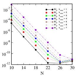
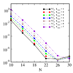
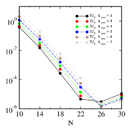
Figure 1: Values of $S\mathcal{E}_{2}$, $V\mathcal{E}_{2}$, and $T\mathcal{E}_{2}$, the composite scalar, vector, and tensor Laplace operator eigenfunction residuals defined in Eqs. (60)–(62), respectively. These values are plotted as functions of the number of grid points $N$ used in each dimension of each of the eight computational sub-domains.

We also define composite residuals to measure how well the divergence and trace identities are satisfied:

$$(V\mathcal{D}_{2})^{2} = \sum_{A=0}^{2}\sum_{k=k^{V(A)}_{\mathrm{min}}}^{k_{\mathrm{max}}}\sum_{\ell=\ell^{V(A)}_{\mathrm{min}}}^{k}\sum_{m=0}^{\ell}\frac{\bigl{(}\|\mathcal{D}^{k\ell m}_{(A)}\|_{2}\bigr{)}^{2}}{3N_{k\ell m}^{\geq}-2k_{\mathrm{max}}-3},$$ (63)

$$(T\mathcal{D}_{2})^{2} = \sum_{A=0}^{5}\sum_{k=k^{T(A)}_{\mathrm{min}}}^{k_{\mathrm{max}}}\sum_{\ell=\ell^{T(A)}_{\mathrm{min}}}^{k}\sum_{m=0}^{\ell}\frac{\bigl{(}\|\mathcal{D}^{k\ell m}_{(A)\,a}\|_{2}\bigr{)}^{2}}{6N_{k\ell m}^{\geq}-8k_{\mathrm{max}}-12},$$ (64)

$$(\mathcal{T}_{2})^{2} = \sum_{A=0}^{5}\sum_{k=k^{T(A)}_{\mathrm{min}}}^{k_{\mathrm{max}}}\sum_{\ell=\ell^{T(A)}_{\mathrm{min}}}^{k}\sum_{m=0}^{\ell}\frac{\bigl{(}\|\mathcal{T}^{k\ell m}_{(A)}\|_{2}\bigr{)}^{2}}{6N_{k\ell m}^{\geq}-8k_{\mathrm{max}}-12}.$$ (65)

Figure 2 illustrates the composite divergence and trace residuals defined in Eqs. (63)–(65). Each curve in each figure represents one of the composite residual norms for a fixed value of $k_{\mathrm{max}}$ as a function of the numerical resolution $N$. These plots illustrate how the values of these residuals depend both on $k_{\mathrm{max}}$ and on the numerical resolution $N$ used to evaluate them.

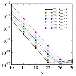
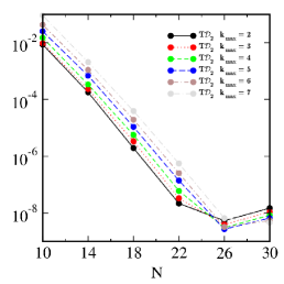
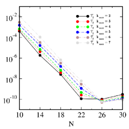
Figure 2: Values of $V\mathcal{D}_{2}$, $T\mathcal{D}_{2}$, and $\mathcal{T}_{2}$, the composite vector and tensor divergence residuals, and tensor trace residual, defined in Eqs. (63)–(65), respectively. These values are plotted as functions of the number of grid points $N$ used in each dimension of each of the eight computational sub-domains.

Finally we define composite residuals that measure how well the ortho-normality residuals are satisfied:

$$(S\mathcal{O}_{2})^{2}=\sum_{k=0}^{k_{\mathrm{max}}}\sum_{\ell=0}^{k}\sum_{m=-\ell}^{\ell}\sum_{k^{\prime}=0}^{k_{\mathrm{max}}}\sum_{\ell^{\prime}=0}^{k^{\prime}}\sum_{m^{\prime}=-\ell^{\prime}}^{\ell^{\prime}}\frac{\left|S\mathcal{O}^{k\ell m}_{k^{\prime}\ell^{\prime}m^{\prime}}\right|^{2}}{N_{k\ell m}^{2}},$$ (66)

$$(V\mathcal{O}_{2})^{2}=\sum_{A=0}^{2}\sum_{B=0}^{2}\sum_{Vk\ell m}^{k_{\mathrm{max}}}\sum_{Vk^{\prime}\ell^{\prime}m^{\prime}}^{k_{\mathrm{max}}}\frac{\left|V\mathcal{O}^{(A)k\ell m}_{(B)k^{\prime}\ell^{\prime}m^{\prime}}\right|^{2}}{\left(3N_{k\ell m}-2k_{\mathrm{max}}-3\right)^{2}},\qquad$$ (67)

$$(T\mathcal{O}_{2})^{2}=\sum_{A=0}^{5}\sum_{B=0}^{5}\sum_{Tk\ell m}^{k_{\mathrm{max}}}\sum_{Tk^{\prime}\ell^{\prime}m^{\prime}}^{k_{\mathrm{max}}}\frac{\left|T\mathcal{O}^{(A)k\ell m}_{(B)k^{\prime}\ell^{\prime}m^{\prime}}\right|^{2}}{\left(6N_{k\ell m}-10k_{\mathrm{max}}-15\right)^{2}},\qquad$$ (68)

where $\sum_{Vk\ell m}^{k_{\mathrm{max}}}$ and $\sum_{Tk\ell m}^{k_{\mathrm{max}}}$ are defined as

$$\sum_{Vk\ell m}^{k_{\mathrm{max}}} = \sum_{k=k^{V(A)}_{\mathrm{min}}}^{k_{\mathrm{max}}}\sum_{\ell=\ell^{V(A)}_{\mathrm{min}}}^{k}\sum_{m=-\ell}^{\ell},$$ (69)

$$\sum_{Tk\ell m}^{k_{\mathrm{max}}} = \sum_{k=k^{T(A)}_{\mathrm{min}}}^{k_{\mathrm{max}}}\sum_{\ell=\ell^{T(A)}_{\mathrm{min}}}^{k}\sum_{m=-\ell}^{\ell},$$ (70)

and where $N_{k\ell m}=(k_{\mathrm{max}}+1)(k_{\mathrm{max}}+2)(2k_{\mathrm{max}}+3)/6$ is the number of $k\ell m$ triplets with $-\ell\leq m\leq\ell$. The terms $2k_{\mathrm{max}}+3$ and $10k_{\mathrm{max}}+15$ that appear in Eqs. (67) and (68) respectively represent the number of terms excluded in these sums by the lower bounds $k\geq k^{T(A)}_{\mathrm{min}}$ and $\ell\geq\ell^{T(A)}_{\mathrm{min}}$.

Figure 3 illustrates the composite ortho-normality residuals defined in Eqs. (66)–(68) for our numerical scalar, vector and tensor harmonics. Each curve represents one of the composite ortho-normality residual norms for a fixed value of $k_{\mathrm{max}}$ as a function of the numerical resolution $N$. These plots illustrate how the values of these residuals depend both on $k_{\mathrm{max}}$ and on the numerical resolution $N$ used to evaluate them. These composite ortho-normality residuals depend on numerical integrals of the $\mathbb{S}^{3}$ harmonics, but not on their numerical derivatives. Consequently these residuals are expected to be much smaller (for fixed $k_{\mathrm{max}}$ and $N$) than the Laplace operator eigenfunction residuals and the divergence residuals.

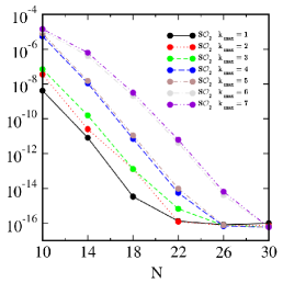
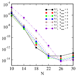
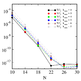
Figure 3: Values of $S\mathcal{O}_{2}$, $V\mathcal{O}_{2}$, and $T\mathcal{O}_{2}$, the composite scalar, vector, and tensor ortho-normality residuals defined in Eqs. (66)–(68), respectively. These values are plotted as functions of the number of grid points $N$ used in each dimension of each of the eight computational sub-domains.

6 Summary

We have summarized the useful properties of the scalar, vector, and tensor harmonics on the three-sphere, and we have presented a new notation that unifies, simplifies and clarifies the analytical expressions for these harmonics. As such, these expressions are in a form that is well-suited for straightforward numerical implementation. We have performed numerical tests of the harmonics computed in this way, and have presented results that demonstrate the accuracy and convergence of the methods.