A new indexed approach to render the attractors of Kleinian groups

Abstract.

One widespread procedure to render the attractor of Kleinian groups, published in the renown book [9] and based upon a combinatorial tree model, wants huge memory resources to compute and store all the words required. We will present here a new faster and lighter version which drops the original words array and pulls out words from integer numbers.

1. Introduction: some definitions

Let $K$ be a group of one-to-one relations. One model binds the elements of $K$ to strings of letters, because these symbols show up in two cases, distinguishing the elements from their inverses: ‘$a$’ (lower case) and ‘$A$’ (upper case).

The generating set $G$ is the smallest subgroup of $K$ such that elements of $K$ are expressed as the combination, termed multiplication, of elements of $G$, often tagged with single letters, and collecting into the alphabet of $K$. Multiplication corresponds, lexically, to concatenation of letters into one string: the so-called word. Words resemble to algorithms, enjoying symbolic (code) and operative (run) features. There are finite ($bbbbaBAbA$) or infinite ($\overline{b}bbbaBAbA$) words and the reading order, left-to-right ($LR$) or right-to-left ($RL$), drives the letters/generators picking. Let $W=abA$ in RL, then $z_{1}=A(z_{0}),z_{2}=b(z_{1}),z_{3}=a(z_{2})$ returns a sequence of values $z_{n}$, the orbit. The last orbit element is defined here as word value. Any subword, returning the identity map $I$, is said crash word, provoking the cancellation of letters and returning a reduced word. Let $W=aBbA$: we have two cancellations, $bB$ and $aA$, and $W$ reduces to $I$.

Words in $K$ converge uniformly to limit cycles, collectively defined as the attractor. Generators and words show up in a twofold (lexical and geometric) nature: as symbol/point and as concatenation/orbit respectively. Such a duality extends to groups, in terms of words/attractor.

2. Basic setup

Working with attractors wants a sufficient degree of freedom and to consider all words in the group. So we step back to the abstraction of strings and symbols, because we need a ‘malleable’ setup to work with: any concatenation of letters up to bounded length $d$. According to the theory of enumerative combinatorics, it is graphically feasible through a $m$-branched tree (see fig. 2), where $m$ is the alphabet length.

Figure 1. Original tree. Enumeration of all possible concatenations of symbols up to depth $2$.

Luckily, the theory of combinatorial groups can set up close links between tree graphs and groups: generators and words interact with the concepts of node, path, depth, root, leaf, parent, child. A comfortable tool to condense the rules of group generation is the presentation. We account two versions: the Cayley multiplication table, for finitely generated groups, including all multiplicative combinations between elements of $G$; and the so-called group presentation, a compact list of generators, the relators $R$, and relations $S$ [7], often of crash kind: $\langle R|S\rangle$. When supported by a presentation, the tree shows as the easiest graphical expedient to explain the group generation. Figure 2 shows the original tree, not related to group presentation. We will work with trees of bounded depth $d<+\infty$.

& (A) (B)

Figure 2. Pruning. (A) New nodes are pruned if producing a crash word (in red). (B) The pruned tree.

3. Once-punctured torus groups

Let $K$ be a Kleinian group, a discrete group of orientation preserving conformal maps $M$. In recent times, this topic gained more interest from the popular audience as it was dragged by the caravan of fractals, due to the close links to Julia sets. Let $M$ be a linear fractional map $(mz+n)/(pz+q)$ in one complex variable $z\in{\mathbb{C}}$. We are interested into the quasi-Fuchsian subfamily of $K$ and we will work with $4$ generators $a,b,A,B$: the topological model is the once-punctured torus and it shows as the free product $K=G*H$, $G=\{a,A\},H=\{b,B\}$. The presentation is $\langle x,X|xX=I\rangle$ or, since Kleinian groups are finitely generated, the Cayley table 1. $K$ is free because no more relations besides trivial ones are listed. We will discuss the role of Cayley table later in section 5. This presentation prunes the original tree in fig. 2 from nodes related to strings with crash words Aa, aA, Bb, bB (fig. 2/A at p. 2) that send points forth and back like in a cycle: $z_{1}=A(z_{0}),z_{0}=a(z_{1})$. Here the identity map halts the branching action of the tree and results only when the next child node has same letter as of its parent, but inverse case. The goal is to have no reduced words (which basically duplicate other nodes) and we get the pruned tree in fig. 2/B.

	I	a	b	A	B
I	$I$	$a$	$b$	$A$	$B$
a	$a$	$a$	$b$	$I$	$B$
b	$b$	$a$	$b$	$A$	$I$
A	$A$	$I$	$b$	$A$	$B$
B	$B$	$a$	$I$	$A$	$B$

Table 1. Cayley multiplication table for once-punctured torus groups.

4. The revised deterministic approach

The problem of rendering the attractor of $K$ has been studied thoroughly, in terms of automatic groups, only in [8, 9], as far as the author knows.

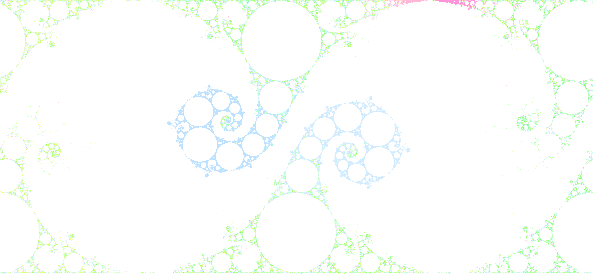
Figure 3. Probabilistic rendering. Attractor for the parameter $\mu=-0.097+1.838i$ in the Maskit T1,1 embedding, rendered via a ‘boosted-up’ modification. Only 1.048.576 words has been required to enhance sharp details.

Two approaches have been developed. One is probabilistic, not relying on tree model and working on one only word/orbit, which gets longer and longer as generators are appended through random picks, given a probability law. The second is deterministic, where words obey to the combinatorial tree model. The larger the depth, the longer the word, the finer the rendering: it is the essential principle of this approach, needing to run millions of words for sharp results. The original implementation casts a huge array of words - the dictionary, demanding a very expensive run, for fine quality results, in terms of memory allocation and addressing. The core of the algorithm is essentially the same as of the original one, so it is not intended to return finer quality renderings.

& (A) (B)

Figure 4. First stage. (A) Numerical paths: the mid row shows numbers composition from 10 to 19. The bottom row shows one next step. (B) Digital version of the lexical pruned tree.

We are going to explain a two-stages strategy revisiting the pruned tree of letters. Numbers are the synthesis of two entities: symbol and value. Consider the set $\{10,11,12,\dots,19\}$ in terms of symbols: the elements come from appending one digit on the right of ‘$1$’, like a new branch of a tree (see fig. 2/A). It makes sense to review numbers in terms of paths. Given the mapping $[a\rightarrow 0,A\rightarrow 1,b\rightarrow 2,B\rightarrow 3]$, we replace letters with digits in the tree at p. 2. Starting from the root at depth 0, corresponding to $I$ (empty string), we move to the left branch at depth $1$ and get the subword ‘$1$’; we route to one of next branches and get ‘$31$’ at depth $2$. Each node binds to a unique path, to one only chain of digits and we pull out the digital tree in fig. 2/B.

The master plan is to move from symbols to digits and finally to indexes (numbers). Now notice that words include digits from $0$ to $m-1$ (here $m=4$) and nodes bind to base-$m$ numbers, turning into indexes in base-10 (prefixed by ‘$\sharp$’ in fig. 5). Indexes count the appearing order of nodes, during the whole tree growth. The notation $31_{4\leftarrow}$ indicates that $31$ is written in base-$4$ and read in RL order: it amounts to $4_{10\leftarrow}$. For example, $Ba\Rightarrow 21_{4\leftarrow}\Rightarrow 5_{10\leftarrow}$. We finally get the indexed tree in fig. 5/A), whose nodes bind to base-$10$ indexes.

Figure 5. Second stage. Indexed version of the digital tree: red nodes mark crash words.

So we do not need to store the words: everything we want is already ‘coded’ inside integer numbers. We have just to count them!

5. Cayley Multiplication Tables

Cayley tables portray all multiplicative combinations between pairs of elements of $G$ and are very intuitive for code implementation: they are homologue to state transition tables and can be supported by a finite state automaton (FSA) to compute word runs [6]. In terms of values, words become dynamical systems whose ‘states’ match to cells value. Cayley tables prune the original tree, depending on whether the final state is of crash kind (indexed with $0$) or not. How ?

	$0$	$1$	$2$	$3$	$4$
$0$	$0$	$1$	$2$	$3$	$4$
$1$	$1$	$1$	$2$	$0$	$4$
$2$	$2$	$1$	$2$	$3$	$0$
$3$	$3$	$0$	$2$	$3$	$4$
$4$	$4$	$1$	$0$	$3$	$4$

Table 2. Zig-zagging for words of once-punctured torus groups. On the left, the indexed version of Cayley table 1. At the center, the succession of states related to the word $abA$, that is, $123$ (RL). On the right, the crash path of word $AabA$.

The Cayley table for once-punctured torus groups is simple to be implemented in terms of coding: its action just resumes into the recognition of crash words $\{aA,Aa,bB,Bb\}$. But there are groups equipped with more complicate presentations, demanding a generalized management. The strategy is to take on each string from the original tree and test its run via the Cayley table. We will work on two examples that progressively generalize concepts.

The once-punctured torus groups offer a comfortable start. The resulting indexes, originally ranging in $[0-9]$, will be incremented by $1$ in order to avoid collisions with the crash state. Let $W=abA$ (RL) and the indexed table 2 at p. 2. $W$ turns into $123$. For algorithmic reasons, the table scan begins from the ‘neutral’ state of the identity element, at row $0$: $WI\equiv W$. We read the first symbol $3$ and we move to column $3$ with state $3$. The sense of a dynamical system is that each state rules the next one: this explains why we will place at row $3$. We read the second symbol $2$, we move to column $2$ with state $2$. We place at row $2$, we read the third symbol $1$ and we move to column $1$, with (final) regular state $1$.

The second example is the Klein-four group, equipped with simple but less obvious presentation: $\langle a,b|a^{2}=b^{2}=(ab)^{2}=I\rangle$. Despite of its name, it has nothing to do with Kleinian groups, but we want to show that the crash state shall be generalized and no longer tied to pairs of inverse letters, as we did for once-punctured torus groups: here each generator is the inverse of itself.

	$I$	$a$	$b$	$ab$
$I$	$I$	$a$	$b$	$ab$
$a$	$a$	$I$	$ab$	$b$
$b$	$b$	$ab$	$I$	$a$
$ab$	$ab$	$b$	$a$	$I$

	$0$	$1$	$2$	$3$
$0$	$0$	$1$	$2$	$3$
$1$	$1$	$0$	$3$	$2$
$2$	$2$	$3$	$0$	$1$
$3$	$3$	$2$	$1$	$0$

Table 3. Klein Four-Group. From left to right, multiplication table, tree model and indexed version of the left table.

We immediately notice a generator labelled with $ab$, a compound word. Turning this Cayley table into the indexed version (table 3, on the right) will keep up the one-to-one symbolism. We ‘expand’ a non-cyclic $3$-branched original tree (like at p. 2) and apply the mapping $[a\rightarrow 1,b\rightarrow 2,ab\rightarrow 3]$ to return the indexed tree. Now we can rework the indexed words via the Cayley table. Let the indexed $W=123$ (RL), which translates back to $(a)(b)(ab)$. The reading will end up at row $1$ / column $1$. The final zero index shows that ‘123’ is a crash word! There are even more complicate groups, as the one with commutators of order $2$ in [9], p. 359: $(abAB)^{2}=I$, including the generators with multiple crash states.

6. Implementation

Disclaimer. As higher level language, Javascript runs reasonably slower than lower level homologous ones, such as C⁺⁺. The fastest algorithms want bare coding: just the strict number of calculations and possibly no external calls. Our web environment has broader goals and does not follow such indications; our benchmarks just attest faster speeds, not the fastest possible. We will show some Javascript pseudo-code implementing the indexed scan.

We count all nodes in the original tree and return the indexed word through the routine get_RL_word. The goal is to return strings whose length is equal to the node depth. This routine does not merely run as the ordinary base conversion. Some tests showed that there could be base-10 indexes which may not retrieve the sought word of required depth and then bug the final rendering. So we put an extra if-statement assuring that the tree is transversed all the way back to depth $1$. Our code is tuned to $9$ generators at most, each one binding to one digit from $1$ to $9$ (and $0$ for $I$). If more than $9$ are required, we shall replace the string out with a specific array object that stores indexes as tokens, because a string – although being an array too – allows to save only one symbol at each position of this data structure.

  RL-path scanner     1 function get_RL_word( _n, _gens_n, _depth ) 2 { 3   // _gens_n : is the number of symbols, i.e. of generators 4   var _rem = 0, _quot = _n, out = "" ; 5   while( true ) 6   { 7     // remainder incremented by 1 to match our indexing 8     // rule: 0 for identity, other digits for generators index 9     _rem = ( _quot % _gens_n ) + 1 ; 10     _quot = ( _quot / _gens_n ) >> 0 ; // integer division 11     //it stops only when depth 1 is reached 12     if ( _quot < _gens_n && _depth <= 1 ) return _rem + ’’ + out ; 13     out = _rem + ’’ + out ; // string concatenation 14     _depth-- ; 15   } 16 }     

We give the code below to check an indexed word run through any Cayley table. It is simply a multi-dimensional array reading, returning $0$ if a crash word is met, otherwise returns $1$.

  Check word run     1 // indexed Cayley table for once-punctured torus groups 2 var _idx_cayley_table = [ [ 0, 1, 2, 3, 4 ], 3                           [ 1, 1, 2, 0, 4 ], 4                           [ 2, 1, 2, 3, 0 ], 5                           [ 3, 0, 2, 3, 4 ], 6                           [ 4, 1, 0, 3, 4 ] ] ; 7  8 function check_word_run( _idx_word, _cayley_table ) 9 { 10  11 // we start from row 0, by convention 12 var _idx = -1, _ret = 1, _row = 0 ; 13  14 /* get the input word, split indexes into tokens, convert’em all 15 into numbers and reverse for RL order */ 16  17 _idx_word=_idx_word.split( "" ) ; 18 _idx_word=_idx_word.map(function(_i){return parseInt(_i,10 );}) ; 19 _idx_word = _idx_word.reverse(); //RL reading order 20  21 for( var _i = 0 ; _i < _idx_word.length ; _i++ ) 22 { 23   _idx = _idx_word[_i], _row = _idx_cayley_table[_row][_idx] ; 24   if ( _row == 0 ) { _ret = 0; break ; } // crash state is met 25 } 26  27 return _idx == -1 ? 0 : _ret ; 28 }     

All nodes will be scanned according to the tree in fig. 5 and keep track of both depth and run for each node. The attractor can be plot in ‘limit set’ or ‘tiling’ rendering mode, whether word points are drawn for leaves only or for all nodes respectively. Given an $m$-branched tree, let $\lambda=m^{d}$ be the number of nodes at bounded depth $d\leq D<+\infty$. The tree counts $\sigma=\sum_{d=1}^{D}\lambda$ or $\lambda=m^{D}$ nodes if the rendering works in ‘tiling’ or in ‘limit set’ mode respectively. We finally code the nested loops below, to render the attractor in four steps: (1) a loop feeding the fixed points to start the orbits; (2) a loop to get the indexed word from each node; (3) a loop to read and compute and draw the word values.

  Index search algorithm     1 var _gens_n = 4, _rl_word = "", _max_depth = 4, _fp = null ; 2 /*assume that we already collected the fixed points of the Mobius 3   transformations of K into the array _input_fixed_pts and that we have 4   a multi-dimensional array storing the current Cayley Table*/ 5 // feed fixed points 6 for( var _p = 0 ; _p < _input_fixed_pts.length ; _p++ ) 7 { 8     _nodes_n = Math.pow( _gens_n, _d ) ; 9     // n is the index of each node belonging to depth _d 10     for( var _n = 0 ; _n < _nodes_n ; _n++ ) 11     { 12       _fp = _input_fixed_pts[_p] ; 13       _rl_word = get_RL_word( _n, _gens_n, _d ) ; 14       // pseudo-code (loop): 15       // 1.0 read _rl_word 16       // 2.0 check_word_run( _rl_word, _cayley_table ) 17       // 2.1 if crash state is met, continue to the next iteration 18       // 2.2 otherwise, for each digit in the _rl_word: 19       // 2.2.1 get the related Mobius transformation M_n. 20       // 2.2.2 apply _fp = M_n(_fp) 21       // 3.0 draw _fp on the screen, according to 22              ’tiling’ (any word) 23              ’limit set’ (only words whose length = depth) mode 24     } 25 }     

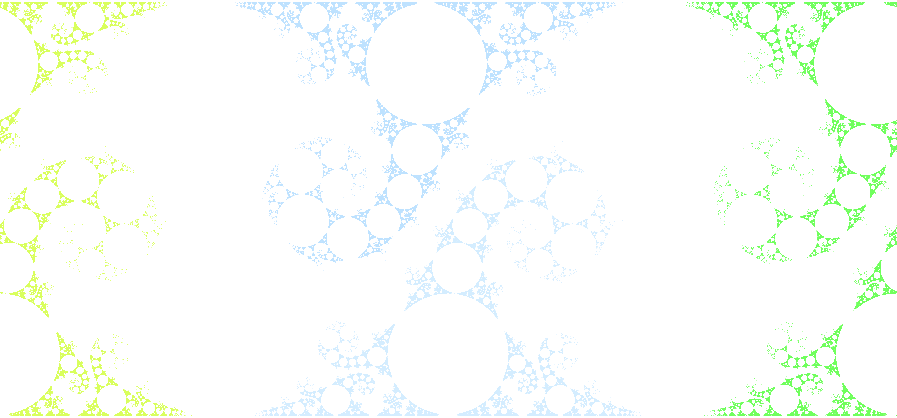
Figure 6. Index-search approach. Same attractor as in picture 3, rendered through a tree of depth $14$, counting about $350$ millions of words. In terms of original deterministic approach, the dictionary would weight more then $4$ Gigabytes.

7. Conclusions

The benefits of this new version of the deterministic approach account to: 1) pull out any word from an integer; 2) save memory resources required by the dictionary array and by calls to outer functions for trasversing the pruned tree; 3) very easy implementation.

The deterministic approach, as well as the probabilistic version, runs too slow long to get fine results at reasonable times: both of them do need some tricks to be accelerated.

References

- [1] Alexander D.S., Iavernaro F., Rosa A., Early days in complex dynamics, AMS, 2011.
- [2] Cayley A., On the theory of groups, as depending on the symbolic equation , Philosophical Magazine, Vol. 7 (1854), pp. 40–47.
- [3] Epstein D., Cannon J., Holt D., Levy S., Paterson M., Thurston W., Word Processing in Groups, Boston, MA, Jones and Bartlett Publishers, 1992.
- [4] Fenwick P.M., A New Data Structure for Cumulative Frequency Tables, Software-Practice and Experience, vol. 24(3), 1994, pp. 327–336.
- [5] Gehring F., Martin G., Discrete quasiconformal groups I, Proceedings of the London Mathematical Society, 55 (1987), pp. 331–358.
- [6] Hopcroft J.E., Ullman J.D., Introduction to Automata Theory, Languages, and Computation, Addison-Wesley, 1979.
- [7] Lyndon R.C., Schupp P.E., Combinatorial Group Theory, Springer-Verlag, 1977.
- [8] McShane G., Parker J.R., Redfern I., Drawing limit sets of Kleinian groups using finite state automata, Experiment. Math. Volume 3, Issue 2 (1994), pp. 153–170.
- [9] Mumford D., Series C., Wright D., Indra’s pearls: The Vision of Felix Klein, Cambridge University Press, 2002 (reprinted in 2015).