Correlation between the luminosity and spin-period changes during outbursts of 12 Be binary pulsars observed by the MAXI/GSC and the Fermi/GBM

Abstract

To observationally study spin-period changes of accreting pulsars caused by the accretion torque, the present work analyzes X-ray light curves of 12 Be binary pulsars obtained by the MAXI/GSC all-sky survey and their pulse periods measured by the Fermi/GBM pulsar project, both covering more than 6 years from 2009 August to 2016 March. The 12 objects were selected because they are accompanied by clear optical identification, and accurate measurements of surface magnetic fields. The luminosity $L$ and the spin-frequency derivatives $\dot{\nu}$, measured during large outbursts with $L\gtsim 1\times 10^{37}$ erg s^-1, were found to approximately follow the theoretical relations in the accretion torque models, represented by $\dot{\nu}\propto L^{\alpha}$ ($\alpha\simeq 1$), and the coefficient of proportionality between $\dot{\nu}$ and $L^{\alpha}$, agrees, within a factor of $\sim 3$, with that proposed by Ghosh & Lamb (1979). In the course of the present study, the orbital elements of several sources were refined.

1 Introduction

X-ray binary pulsars (XBPs) are systems consisting of magnetized neutron stars and mass-donating stellar companions. In the vicinity of the neutron star, matter flows from the companion are guided by the magnetic fields, and are finally funneled onto the magnetic poles of the neutron star. Because the accreting matter meanwhile transfers its angular momentum to the neutron star, the pulsar’s period-change rate should correlate with the mass accretion rate, i.e. the X-ray luminosity. The relation is thought to reflect the mode of accretion flows, whether thin-disk or nearly spherical, and also the fundamental neutron-star parameters including the mass, radius, and magnetic fields. Consequently, this important issue has been studied from both theoretical and observational points of view.

From theoretical viewpoints, Ghosh & Lamb (1979a, 1979b, hereafter GL79) developed a comprehensive theoretical model, which extends those proposed by Lamb et al. (1973) and Rappaport & Joss (1977). The GL79 model assumes that magnetic field lines from the neutron star thread the disk in a broad transition zone. Then, Wang (1987, 1995), Lovelace et al. (1995, hereafter LRB95), Kluźniak & Rappaport (2007, hereafter KR07), and other authors proposed their revised models, which assume different physical conditions (see Bozzo et al. (2009), Shi et al. (2015), and references therein).

Although a number of observations have so far been performed to examine how the period changes of XBPs depend on their luminosities (e.g. Finger et al. (1996); Reynolds et al. (1996); Bildsten et al. (1997)), the results are still inconclusive to answer whether the phenomenon can be adequately explained by any of the proposed theoretical models, and if so, whether they can be differentiated. This is mainly because these observations have been limited in the sample size, used different energy bands, or employed different assumptions. To obtain a clearer result, we need to carry out unified observations of a reasonable number of objects that satisfy the following four requirements. First, the sample objects must show relatively large changes in their X-ray fluxes, so that the effects of accretion torque are clearly manifested in their spin period changes. Second, the objects must have well established orbital elements (to remove the orbital Doppler effects in their period changes), and reasonably accurate distances (to convert the flux to the mass accretion rate). Third, we need to have preliminary knowledge of the objects’ magnetic-field strength, because this is a key quantity that determines the efficiency of the angular-momentum transfer from the accreting matter to the neutron star. Finally, we need to measure the X-ray intensity, spin period, and the period-change rate of the sample objects for a sufficiently long time in a unified manner.

The first requirement for our study, i.e., large intensity changes, is accomplished by focusing on Be XBPs. Being one of the major XBP subclasses, they form binaries with Be companion stars, which host a circumstellar disk along their equator (e.g. Reig (2011)). These XBPs often exhibit large outbursts lasting for a few weeks to a few months, mostly at a limited orbital phase near the pulsar periastron passage. These outbursts, together with spin-up episodes which are often associated with them (e.g. Bildsten et al. (1997)), are naturally explained by an increase in the accretion rate as the pulsar gets through the stellar disk, and the associated increase in transfer of the angular momentum to the neutron star. If the luminosity and the spin-period changes are monitored throughout these outbursts, the obtained data will become of great value. As detailed later in section 2.3, a fair fraction of the currently known Be XBPs have known orbital parameters and estimated distances. As a result, our second requirement is satisfied automatically.

The third requirement, i.e. the surface magnetic field of neutron stars in XBPs, is best measured with the cyclotron-resonance scattering feature (CRSF) in X-ray spectra (e.g. Makishima et al. (1999)). Thanks to the recent high-sensitivity instruments covering the hard X-ray band onboard the INTEGRAL, Suzaku, and NuSTAR satellites, the number of XBPs with confirmed CRSFs increased in these years (e.g. Yamamoto et al. (2011), Klochkov et al. (2012), Yamamoto et al. (2014), Tendulkar et al. (2014), Marcu-Cheatham et al. (2015), Tsygankov et al. (2016)). So far, the CRSF has been detected from about 25 XBPs altogether, of which 15 are Be XBPs (e.g. Revnivtsev & Mereghetti (2015); Walter et al. (2015)). Therefore, focusing on Be XBPs will also satisfy the third requirement.

Let us consider the final requirement. Since 2009, the MAXI (Monitor of All-sky X-ray Image; Matsuoka et al. (2009)) mission on the International Space Statin has been scanning the whole X-ray sky every 92-minute orbital cycle with the GSC (Gas Slit Camera; Mihara et al. (2011)). Meanwhile, the GBM (Gamma-ray Burst Monitor; Meegan et al. (2009)) onboard the Fermi Gamma-Ray Space Telescope has been monitoring the whole sky in the X-ray to gamma-ray band since 2008. The timing analysis of the GBM data provides us information on the pulsed emission from bright XBPs in our Galaxy (Finger et al., 2009; Camero-Arranz et al., 2010). Data taken by these two missions for over 6 years satisfy the requirement. In fact, we analyzed the data of two XBPs, GX 304$-$1 (Sugizaki et al., 2015) and 4U 1626$-$67 (Takagi et al., 2016), and found that the results on both these sources agree reasonably with the disk-accretion model proposed by GL79.

In the present paper, we investigate the correlation between the luminosity and pulse-period changes of 12 Be XBPs using the long-term ($>6$ years) X-ray data, which were obtained by the MAXI GSC survey and the Fermi GBM pulsar project. The observations and target selection are described in section 2, and the analysis in section 3. We discuss the obtained results in section 4.

2 Observations

2.1 MAXI GSC

Since the MAXI in-orbit operation started in 2009 August, the GSC light curves of $\sim 300$ pre-registered sources have been processed, typically every day, in the 2–4 keV, 4–10 keV, and 10–20 keV bands, and the results are uploaded on the archive web site. The data provide 3-energy-band photon fluxes for each scan transit of 30–50 s duration, every 92 minutes synchronized with the ISS orbital cycle, as well as those averaged for every MJD (Modified Julian Date) time bin. In the standard data processing, the time-dependent effective area for each target is calculated by assuming that it has a nominal Crab-like spectrum, in the 2–20 keV band, represented by a power-law with a photon index $\Gamma=2.1$. Among these sources, some 52 are XBPs; their long-term ($\gtsim 6$ years) intensity histories can be constructed from the GSC data.

We can also analyze X-ray energy spectra of bright sources using all available event data from the MAXI GSC. Together with the distance, this information is necessary to quantitatively estimate the bolometric source luminosity, and hence the accretion rate. The GSC response functions are calculated with the standard tools (Sugizaki et al., 2011; Nakahira et al., 2012), and the model fits to the GSC spectra are carried out on the XSPEC software version 12.8 (Arnaud, 1996) released as a part of the HEASOFT software package, version 6.19.

Since the MAXI GSC scans over each target on the sky only for 30–50 s every 92 minutes, it is not suited for pulse-period measurements, unless the period is $\lesssim 30$ s or longer than $\gtsim 92$ min (e.g. Takagi et al. (2016)). Therefore, we rely on the Fermi GBM data as described below.

2.2 Fermi GBM pulsar data

The Fermi GBM pulsar project (Finger et al., 2009; Camero-Arranz et al., 2010) provides, on their web site, results of the timing analysis for pulsating X-ray sources in the energy band above 8 keV. The data consist of pulse frequencies and pulsed fluxes of positively detected $\sim 50$ XBPs in our Galaxy and the Large Magellanic Cloud (LMC), obtained since the in-orbit operation started in 2008 July. When the binary orbital elements of the objects are accurately known, the released pulse periods are already corrected for the expected orbital Doppler shifts. We utilize the pulse frequency data of the Be XBPs to be studied, but not their pulsed fluxes.

2.3 Target selection

The high-mass X-ray binary catalogues, given by Liu et al. (2006) and Walter et al. (2015), list 60 Be X-ray binaries and its candidates in our Galaxy. Out of them, 29 objects have securely been established as Be XBPs bases on the detection of periodic X-ray pulsations and the optical identification with Be-star companions. These objects hence constitute a starting point of our sample, because Be XBPs are considered to provide an ideal opportunity for our purpose (section 1).

Among the 29 Be XBPs, the GBM have detected significant pulsed emission from 14 sources, each at least on one occasion, since the MAXI in-orbit operation started in 2009. Table 1 lists their source names, pulse periods, orbital periods and eccentricities, spectral types of their optical companions, and the source distances estimated from the optical data. The table also gives the time period over which each source was positively detected by both the MAXI/GSC and the Fermi/GBM.

Among these 14 objects, the binary orbital elements (as represented by the eccentricity in table 1) are still unavailable for two sources, Cep X-4 and LS V $+$44 17. Therefore, we cannot remove the orbital Doppler effects from their pulse-period data. Furthermore, useful period-change measurements require the source to be detected over a sufficiently long period, typically 10 days. As seen in table 1, the data of two other sources, MXB 0656-072 and SAX J2103.5+4545, do not satisfy the condition. We thus excluded these four sources, and chose the remaining 11 Be XBPs as the primary analysis targets.

In addition to these, we included, into our final sample, one more object, RX J0520.5$-$6547, which is not in our Galaxy but in the LMC. It showed a large outburst activity in 2013–2014, which was observed by both the GSC and the GBM, and also allowed the CRSF detection (Tendulkar et al., 2014). Table 1 hence includes data of the object.

Among the 12 objects in our final sample, the CRSF has been detected from 9 sources. The surface magnetic field $B_{12}$ in units of $10^{12}$ G is estimated from the fundamental CRSF energy $E_{\mathrm{a}}$ as

$$B_{12}=\frac{1}{\sqrt{1-x^{-1}}}\left(\frac{E_{\mathrm{a}}}{\mathrm{11.6\,keV}}\right)$$ (1)

where

$$x=\frac{Rc^{2}}{2GM}$$ (2)

is the surface redshift parameter, namely, the ratio of the neutron-star radius $R$ to the Schwarzschild radius, with the neutron-star mass $M$, the gravitational constant $G$, and the velocity of light $c$. In several XBPs, the observed $E_{\mathrm{a}}$ values are known to depend to some extent on the source luminosity (Mihara et al., 2004; Nakajima et al., 2006, 2010; Yamamoto et al., 2011; Klochkov et al., 2012). This behavior is understood by considering that the scattering region responsible for the CRSF formation changes its height along the field lines, depending on the balance between the radiation and accretion pressures (Mihara et al., 1998; Staubert et al., 2007). To best estimate the field strength on the neutron-star surface, we employed the highest $E_{\mathrm{a}}$ value that has ever been recorded in each source. In table 1, the selected $E_{\mathrm{a}}$ values from the past literature are listed.

Table 1: Properties of Be XBPs detected by Fermi GBM and MAXI GSC since 2009 August 15 to 2015 December 31.

∗No.	Source name	†$P_{\rm s}$	†$P_{\rm orb}$	†$e$	Active epoch	†$T_{\rm out}$	Spec.Type	†$D$	†$E_{\rm a}$
		( s )	( d )		( MJD )	( d )		(kpc)	(keV)
1	4U 0115$+$63	3.6	24.3	0.34∗1	55701 – 57343	64.9	B0.2 Ve∗2	$7.0\pm 0.3$∗44	$16$∗3,4
2	X 0331$+$53	4.4	33.9	0.37∗5	57193 – 57290	56.0	O8.5 Ve∗6	$6.0\pm 1.5$∗45	$31$∗7
3	RX J0520.5$-$6932	8.0	23.93	0.03∗8	56644 – 56725	77.9	O8 Ve∗9	$50\pm 2$∗9	$31.5$∗10
4	H 1553$-$542	9.3	31.34	0.04∗12	57046 – 57144	94.0	B1-2 V∗11	$20\pm 4$∗11	$27.3$∗12
5	GS 0834$-$430	12.3	105.8	0.12∗14	56106 – 56146	34.0	B0-2 III-Ve∗13	$5^{+1}_{-2}$∗13	—
6	XTE J1946$+$274	15.8	172.0	0.33∗15	55352 – 55682	119.9	B0–1 IV–Ve∗16	$8.7\pm 1.2$∗44	$35$∗17,15
7	2S 1417$-$624	17.5	42.2	0.45∗18	55124 – 55218	94.0	B1 Ve∗19	$11^{+1}_{-9}$∗19	—
8	KS 1947$+$300	18.8	40.4	0.02∗20	56567 – 57089	135.9	B0 Ve∗21	$10.4\pm 0.9$∗44	$12.2$∗22
9	EXO 2030$+$375	41.3	46.0	0.41∗23	55057 – 57279	368.4	B0e∗24	$6.5\pm 2.5$∗45	—
$\cdot$	Cep X-4∗	66.3	—	—	56813 – 56843	6.0	B1-B2 Ve∗25	$5.9\pm 0.9$∗44	$30.4$∗26,27
10	GRO J1008$-$57	93.7	249.5	0.68∗28	55157 – 57170	365.4	B0e∗29	$5.8\pm 0.5$∗44	$76$∗30
11	A 0535$+$262	103.5	111.1	0.47∗31	55050 – 57070	245.6	O9.7 IIIe∗32	$2.1\pm 0.5$∗32	$46.8$∗33,34
$\cdot$	MXB 0656$-$072∗	160.7	101.2	—	55288 – 55292	3.9	O9.7 Ve∗35	$3.9\pm 0.1$∗35	$32.8$∗35
$\cdot$	LS V $+$44 17∗	205.2	—	—	55284 – 55716	33.9	B0.2 Ve∗36	$2.2\pm 0.5$∗36	$31.9$∗37
12	GX 304$-$1	275.5	132.2	0.52∗38	55286 – 57145	209.1	B0.7 Ve∗39	$2.4\pm 0.5$∗40	$53.7$∗41
$\cdot$	SAX J2103.5$+$4545∗	358.6	12.7	0.4∗42	55483 – 56965	23.9	B0 Ve∗43	$6.5\pm 0.9$∗43	—

^∗ Objects with numbers (1–12) constitute our final sample. ^†$P_{\rm s}$, ^†$P_{\rm orb}$, ^†$e$, ^†$T_{\rm out}$, ^†$D$, and ^†$E_{\rm a}$ are the pulse period, the orbital period, the orbital eccentricity, the total period for which both the MAXI GSC and the Fermi GBM detected the source, the source distance estimated from the optical companion, and the fundamental cyclotron-resonance energy, respectively.
References: *1. Bildsten et al. (1997), *2. Negueruela & Okazaki (2001), *3. Mihara et al. (2004), *4. Nakajima et al. (2006), *5. Doroshenko et al. (2016), *6. Negueruela et al. (1999), *7. Nakajima et al. (2010), *8. Kuehnel et al. (2014), *9. Coe et al. (2001), *10. Tendulkar et al. (2014), *11. Lutovinov et al. (2016) *12. Tsygankov et al. (2016), *13. Israel et al. (2000), *14. Wilson et al. (1997), *15. Marcu-Cheatham et al. (2015), *16. Verrecchia et al. (2002), *17. Heindl et al. (2001), *18. İnam et al. (2004), *19. Grindlay et al. (1984), *20. Galloway et al. (2004), *21. Negueruela et al. (2003), *22. Fürst et al. (2014), *23. Wilson et al. (2008), *24. Coe et al. (1988), *25. Bonnet-Bidaud & Mouchet (1998) *26. Mihara et al. (1991) *27. Fürst et al. (2015) *28. Kühnel et al. (2013), *29. Coe et al. (1994), *30. Yamamoto et al. (2014), *31. Finger et al. (1996), *32. Steele et al. (1998), *33. Terada et al. (2006), *34. Caballero et al. (2007), *35. McBride et al. (2006) *36. Reig et al. (2005) *37. Tsygankov et al. (2012) *38. Sugizaki et al. (2015), *39. Mason et al. (1978), *40. Parkes et al. (1980), *41. Yamamoto et al. (2011), *42. Baykal et al. (2000) *43. Reig et al. (2004) *44. Riquelme et al. (2012), *45. Reig & Fabregat (2015),

3 Analysis

3.1 X-ray light curves and pulse-frequency changes

Figure 1 show the 2–20 keV light curves of the selected 12 Be XBPs, measured by the MAXI GSC, from 2009 August to 2016 March, and the pulse-frequency $\nu_{\mathrm{s}}$ measured with the Fermi GBM during outbursts in the same period. All the pulse frequencies are first converted to their barycentric values, and then corrected for the orbital Doppler effects, to so-called “spin frequencies”, employing the orbital elements summarized in table 2. These corrections were performed, prior to the data release, by the Fermi/GBM team, expect for GS 0834$-$430, GRO J1008$-$57 and XTE J1946$+$274 for which the orbital parameters were unavailable. Since the orbital parameters of two of them, GRO J1008$-$57 and XTE J1946$+$274, were later published (see references in table 2), we conducted the orbital Doppler corrections by ourselves using the reported parameters.

Through this analysis process, we found that the spin frequencies of 4U 0115$+$63, GS 0834$-$430, KS 1947$+$300, and GRO J1008$-$57 show, as presented in figures 7–9 in Appendix, some modulations synchronized with the binary period, even though the data had already been corrected for the orbital Doppler shifts. This means that the orbital effects may not have been adequately removed. As described in Appendix, the present study allows us to refine the orbital elements in a self-consistent way. Then, as listed in table 2 (in comparison with the previous values), we successfully improved the orbital parameters of these sources, and by employing them, the residual orbital modulations were removed (figures 7–9). The refined spin-frequency data are used in figure 1 and all the analysis hereafter.

Table 2: Binary orbital elements of the selected Be X-ray binary pulsars.

No.	Source name	$P_{\rm orb}$	∗$a_{\rm X}\sin i$	$e$	∗$\omega$	∗$T_{\rm peri}$ (P) or ∗$T_{\pi/2}$ (T)		Ref.& Note
		( d )	( lt-s )		( ∘ )	( MJD )
1	4U 0115$+$63	24.31704(6)	140.13(8)	0.3402(2)	47.66(9)	49279.268(3)	P	[1]
$\cdot$	—	2.431689	141.37	0.3401	49.225	55601.751	P	Appendix
2	X 0331$+$53	33.850(3)	77.8(2)	0.371(5)	277.4(1)	57157.38(5)	P	[2]
3	RX J0520.5$-$6932	23.93(7)	107.6(8)	0.029(10)	233(18)	56666.41(3)	T	[3]
4	H 1553$-$542	31.303(27)	201.3(8)	0.0351(22)	163.4(35)	57088.921(19)	T	[4]
5	GS 0834$-$430	105.8(4)	128(40)	0.12(+8/-4)	140(40)	48809.6(1.5)	T	[5]
$\cdot$	—	105.8 : fix	199	0.125	165	56130.0	P	Appendix
6	XTE J1946$+$274	172.7(6)	471(+3/-4)	0.246(9)	273(2)	55514(1)	P	[6]
7	2S 1417$-$624	42.175	188(2)	0.446(2)	300.3(6)	51612.17(5)	P	[7,8]
8	KS 1947$+$300	40.415(7)	137.4(1.2)	0.034(7)	33(3)	51985.31(7)	T	[9]
$\cdot$	—	40.50	130.2	0.008	57	56550.54	T	Appendix
9	EXO 2030$+$375	46.0213(3)	246(2)	0.410(1)	211.9(4)	52756.17(1)	P	[10]
10	GRO J1008$-$57	249.480(4)	530(6)	0.68(2)	334(8)	55424.7(2)	P	[11, 12]
$\cdot$	—	249.480 : fix	691	0.65	299	55413	P	Appendix
11	A 0535$+$262	111.10	267(13)	0.47(2)	130(5)	53613.00	P	[13]
12	GX 304$-$1	132.189(2)	498(6)	0.524(7)	122.5(4)	55425.020(1)	P	[14]

^∗$a_{\rm X}\sin i$ is the semi-major axis projected on the line of sight. ^∗$\omega$ is the argument of periastron. ^∗$T_{\rm peri}$ (P) or $T_{\rm\pi/2}$ (T) is the epoch of periastron passage or mean logitude of $90^{\circ}$, respectively. The other symbols have the same meanings as in table 1.
References: [1] Bildsten et al. (1997), [2] Doroshenko et al. (2016), [3] Kuehnel et al. (2014), [4] Tsygankov et al. (2016), [5] Wilson et al. (1997), [6] Marcu-Cheatham et al. (2015), [7] Finger et al. (1996), [8] İnam et al. (2004), [9] Galloway et al. (2004), [10] Wilson et al. (2008), [11] Coe et al. (2007), [12] Kühnel et al. (2013), [13] Finger et al. (1996), [14] Sugizaki et al. (2015),

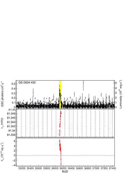
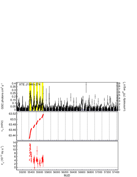
Figure 1: MAXI GSC 2–20 keV light curve in 1-d time bin (top), Fermi GBM pulse frequency corrected for the orbital Doppler shift during outbursts (middle), and frequency derivative (bottom), for each of the 12 selected Be XBPs. All vertical error bars represent 1-$\sigma$ (68 %) confidence limits of statistical uncertainty. The right-side ordinate at the top panel represents the bolomatric luminosity scale calculated from the best-fit spectral models. Vertical dashed lines in the middle panels indicate the epochs of the pulsar periastron passages.

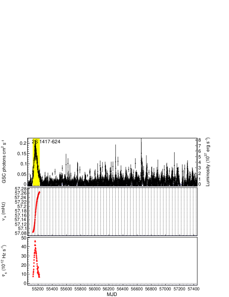
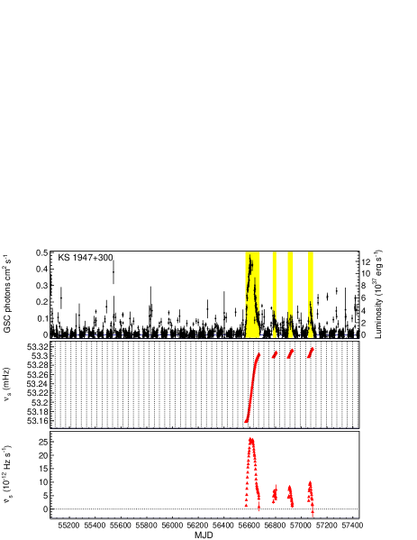
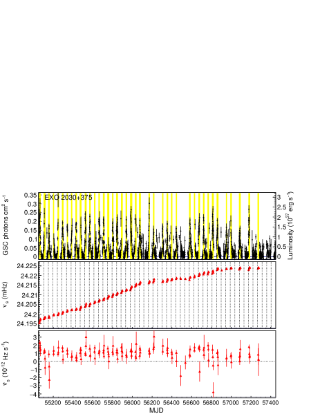
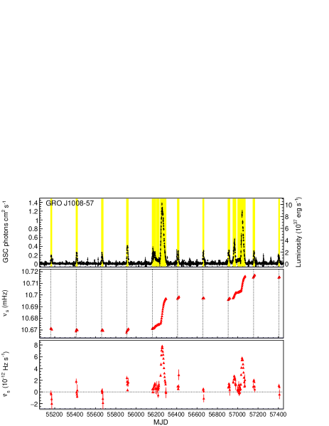
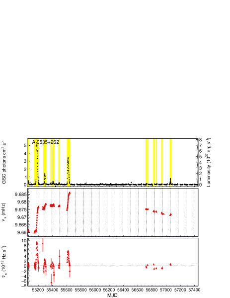
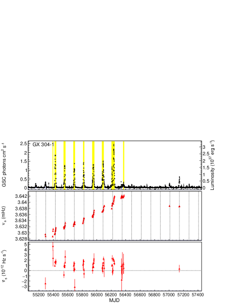
Figure 1: (Continued)

3.2 Pulse-frequency derivative

Figure 1 clearly shows a common behavior that the spin frequency increases, i.e. the pulsar spins up, during each outburst activity. We then calculated the pulse-frequency derivative, $\dot{\nu}_{\mathrm{s}}$, in the following way. In the publicly available GBM pulsar data, the pulse periods of various XBPs are determined typically every 2-d interval. The obtained pulse periods are subject to uncertainties which are mainly due to the limitations in the statistics and the time intervals. Considering these effects, we determined $\dot{\nu}_{\mathrm{s}}$ every 6-d interval by fitting several period measurements in that interval with a linear function, and then estimate the 1-$\sigma$ statistical error, $\sigma_{\nu\mathrm{dot}}$, with the $\chi^{2}$ method.

The obtained values of $\dot{\nu}_{\mathrm{s}}$ are also plotted in figure 1 at the bottom panels. As expected, the time variations of $\dot{\nu}_{\mathrm{s}}$ clearly resemble those of the X-ray intensity at the top panels.

3.3 X-ray spectrum and bolometric luminosity estimate

For the present study, we need to estimate the instantaneous source luminosity from the GSC light curve data. The factor of conversion from the observed count rate to the source luminosity depends on the emission energy spectrum as well as the instrument response function. Hence, we analyzed the GSC energy spectra of the 12 sources, assuming that the energy spectrum of each source does not change significantly over the outburst active periods. Thus, for each source, the spectrum was averaged over all outburst periods, which is defined as the periods wherein the GBM data are available.

Figure 2 shows the 2–30 keV spectra of the 12 sources, thus obtained with the GSC. The background has been subtracted, but the instrumental responses are still inclusive. We fitted them with a typical model for XBPs, consisting of a high-energy-cutoff power-law (PLCUT) continuum, and a Gaussian for iron-K line emission at 6.4 keV (e.g. Makishima et al. (1999); Coburn et al. (2002)). The former is specified by the photon index $\Gamma$, the cutoff energy $E_{\mathrm{cut}}$. the folded energy $E_{\mathrm{fold}}$, and the normalization $A$ as

$$F_{\mathrm{PLCUT}}(E)=\left\{\begin{array}[]{ll}AE^{-\Gamma}&(E\leq E_{\mathrm{cut}})\\ AE^{-\Gamma}\exp\left(-\frac{E-E_{\mathrm{cut}}}{E_{\mathrm{fold}}}\right)&(E_{\mathrm{cut}}<E).\end{array}\right.$$ (3)

Because of the limited energy resolution of the GSC, the centroid and width of the Gaussian were fixed at their typical values, 6.4 keV and 0.1 keV, respectively. To account for the interstellar absorption, a photoelectric absorption factor by a medium with Solar abundances and a free equivalent-hydrogen column density $N_{\mathrm{H}}$ was multiplied. The overall model is thus expressed as phabs*(gaussian + highecut*powerlaw) in the XSPEC terminology.

The PLCUT model was accepted, within 90 % confidence limits of statistic uncertainty, by the GSC spectra of the 11 objects except for X 0331$+$53. In figure 2, the best-fit model folded with the instrument response is shown together with the data, and the data versus model residuals are presented at the bottom panels. Table 3 summarizes the best-fit model parameters.

The residuals of X 0331$+$53 bear an absorption feature at around 25 keV, which made the fit unacceptable with the reduced chi-squared of $\chi^{2}_{\nu}=3.6$ for 31 DOF (degree of freedom). This must be the fundamental CRSF detected in past outbursts (e.g. Makishima et al. (1990); Nakajima et al. (2010)). We then multiplied a cyclotron absorption (CYAB) model (cyclabs in XSPEC terminology; Makishima et al. (1990)) to the PLCUT model, to find that the fit becomes acceptable within the 90% confidence limit. In figure 2, the residuals from the fit with the PLCUT$*$CYAB model are shown together. The best-fit CYAB parameters (table 4) are consistent with those obtained in the past outbursts.

Using the best-fit models and the GSC response functions, we calculated the factors of conversions $f_{\mathrm{bol}}$ from the 2–20 keV count rates to the 0.1–100 keV fluxes (considered to approximate the bolometric flux) corrected for the interstellar absorption. The obtained values are presented in table 3, together with their 68% confidence uncertainties caused by the fitting errors. Further denoting the beaming factor (the observed flux divided by the spherically averaged flux) as $f_{\mathrm{b}}$ and the source distance as $D$, the 0.1–100 keV luminosity $L_{\mathrm{obs}}$ is calculated from the observed 2–20 keV count rate $C_{\mathrm{2-20}}$ as

$$L=4\pi D^{2}f_{\mathrm{b}}f_{\mathrm{bol}}C_{\mathrm{2-20}}.$$ (4)

In figure 1 (top), the ordinate on the right-hand side represents the luminosity scale obtained by assuming $D$ from the optical companion (table 2), $f_{\mathrm{b}}=1$ (isotropic emission), and the value of $f_{\mathrm{bol}}$ as obtained above. The validity of these assumptions is evaluated in section 4. To make coincident samplings of $L$ and $\nu_{\mathrm{s}}$, the $L$ calculation via equation (4) was performed over the same 6-d intervals as for the determination of $\nu_{\mathrm{s}}$.

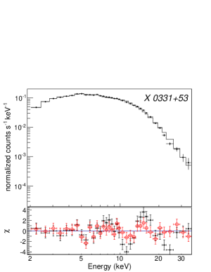
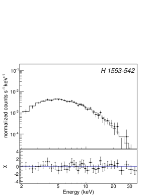
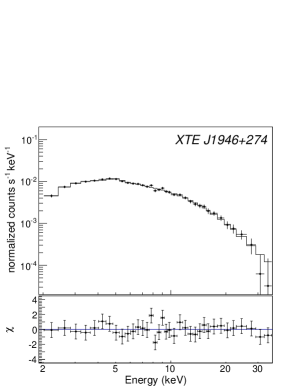
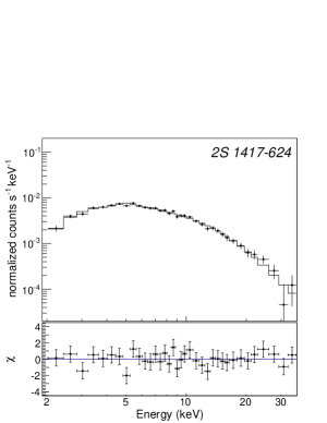
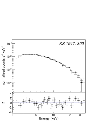
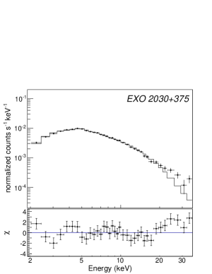
Figure 2: (Top panels) GSC 2-30 keV spectra of the selected 12 Be XBPs, averaged over the entire outburst period, compared with the best-fit PLCUT model folded with the detector response (solid line). Crosses represent statistical 1-$\sigma$ errors. (Bottom panles) Date versus model residuals. In X 0331$+$53, the red points represent those from the PLCUT * CYAB model.

Table 3: Summary of the best-fit spectral parameters^∗.

No.	Source ID	$N_{\rm H}$	$\Gamma$	$E_{\rm cut}$	$E_{\rm fold}$	$EW_{\rm FeK}$†	$\chi^{2}_{\nu}(\nu)$	$F_{\rm 2-20}$‡	$F_{\rm bol}$§	$f_{\rm bol}$∥
		$10^{22}$ cm-2		(keV)	(keV)	(eV)
1	4U 0115	$0.7^{+0.5}_{-0.5}$	$0.5^{+0.1}_{-0.1}$	$8.9^{+0.5}_{-0.5}$	$5.7^{+0.6}_{-0.6}$	$<112$	1.41(30)	$25.7^{+0.4}_{-0.4}$	$36.9^{+1.9}_{-1.8}$	$1.44^{+0.08}_{-0.07}$
2	X 0331	$0.2^{+***}_{-***}$	$0.4^{+***}_{-***}$	$10.9^{+***}_{-***}$	$7.2^{+***}_{-***}$	$<0$	3.73(30)	$163^{+***}_{-***}$	$283^{+***}_{-***}$	$1.74^{+***}_{-***}$
	X 0331#	$<0.2$	$0.3^{+0.0}_{-0.0}$	$8.6^{+0.7}_{-0.9}$	$19.7^{+18.5}_{-6.3}$	$134^{+41}_{-43}$	1.09(27)	$161^{+2}_{-2}$	$652^{+457}_{-199}$	$4.04^{+2.84}_{-1.23}$
3	RX J0520.5	$<0.9$	$1.0^{+0.2}_{-0.1}$	$11.4^{+2.1}_{-3.1}$	$6.0^{+6.5}_{-3.5}$	$170^{+163}_{-167}$	0.72(30)	$5.3^{+0.2}_{-0.2}$	$7.0^{+1.9}_{-0.9}$	$1.32^{+0.35}_{-0.18}$
4	H 1553	$1.9^{+1.8}_{-1.7}$	$<0.4$	$7.5^{+2.5}_{-1.7}$	$9.5^{+7.5}_{-3.0}$	$<236$	0.62(30)	$4.2^{+0.2}_{-0.2}$	$7.0^{+1.8}_{-1.2}$	$1.66^{+0.43}_{-0.28}$
5	GS 0834	$<0.7$	$0.8^{+0.1}_{-0.3}$	$<4.2$	$38^{+47}_{-14}$	$<105$	1.27(30)	$20.8^{+0.5}_{-0.5}$	$66.8^{+13.1}_{-10.9}$	$3.21^{+0.63}_{-0.52}$
6	XTE J1946	$<0.6$	$0.8^{+0.1}_{-0.2}$	$<2.7$	$22^{+11}_{-6}$	$<137$	0.61(30)	$12.2^{+0.3}_{-0.3}$	$30.3^{+5.0}_{-4.1}$	$2.48^{+0.41}_{-0.34}$
7	2S 1417	$1.6^{+1.2}_{-1.4}$	$0.6^{+0.2}_{-0.6}$	$7.5^{+2.3}_{-3.9}$	$16.5^{+9.6}_{-5.7}$	$<186$	0.74(30)	$7.8^{+0.2}_{-0.2}$	$20.0^{+3.7}_{-3.1}$	$2.55^{+0.48}_{-0.40}$
8	KS 1947	$0.7^{+0.4}_{-0.4}$	$1.2^{+0.1}_{-0.1}$	$8.3^{+1.7}_{-1.3}$	$27^{+18}_{-8}$	$106^{+78}_{-80}$	1.42(30)	$15.1^{+0.3}_{-0.3}$	$31.3^{+4.3}_{-3.5}$	$2.07^{+0.28}_{-0.23}$
9	EXO 2030	$0.9^{+0.7}_{-0.7}$	$0.6^{+0.2}_{-0.3}$	$4.1^{+0.6}_{-0.5}$	$10.7^{+4.4}_{-2.8}$	$99^{+55}_{-57}$	1.81(30)	$8.7^{+0.1}_{-0.1}$	$15.3^{+2.2}_{-1.7}$	$1.75^{+0.25}_{-0.20}$
10	GRO J1008	$1.6^{+0.3}_{-0.4}$	$1.0^{+0.1}_{-0.1}$	$7.5^{+0.6}_{-0.8}$	$13.1^{+1.6}_{-1.5}$	$114^{+46}_{-52}$	1.01(30)	$24.4^{+0.2}_{-0.2}$	$44.9^{+2.0}_{-2.0}$	$1.84^{+0.08}_{-0.08}$
11	A 0535	$1.0^{+0.2}_{-0.3}$	$0.9^{+0.1}_{-0.1}$	$8.2^{+0.9}_{-1.3}$	$24^{+3}_{-3}$	$53^{+34}_{-45}$	0.91(30)	$48.9^{+0.3}_{-0.3}$	$129^{+4}_{-4}$	$2.63^{+0.09}_{-0.08}$
12	GX 304	$2.2^{+0.3}_{-0.3}$	$1.0^{+0.1}_{-0.1}$	$7.2^{+0.5}_{-0.5}$	$13.3^{+1.2}_{-1.2}$	$96^{+37}_{-36}$	1.70(30)	$52.2^{+0.3}_{-0.3}$	$98.1^{+3.0}_{-3.1}$	$1.88^{+0.06}_{-0.06}$

^∗All errors represent 90% confidence limits of statistical uncertainty.
^†Equivalent width of iron K (6.4 keV) line
^‡Units in photons cm^-1 s^-1
§Units in $10^{-11}$ erg cm^-1 s^-1
∥Units in $10^{-8}$ erg counts^-1
#CYAB model is applied. The best-fit parameters of the CYAB model are in table 4.

Table 4: CYAB model parameters in X 0331$+$53

$E_{\rm a}$ (keV)	$W$ (keV)	$D$
$23.4^{+1.0}_{-0.8}$	$6.2^{+2.5}_{-2.3}$	$2.0^{+0.8}_{-0.5}$

3.4 Relation between the luminosity and the spin-frequency derivative compared with theoretical models

We have so far derived $\dot{\nu}_{\mathrm{s}}$ and $L$ of the selected 12 Be XBPs, on almost daily basis during the outbursts since 2009 August. Figure 3 shows their relation, called $\dot{\nu}_{\mathrm{s}}$-$L$ diagram, for each of the 12 sources. All diagrams clearly reveal the expected positive correlations between $\dot{\nu}_{\mathrm{s}}$ and $L$, indicating that the pulsars indeed spin up by the accretion torque. Furthermore, in a fair fraction of the 12 objects, the correlation is close to a direct proportionality ($\dot{\nu}_{\mathrm{s}}\propto L$) in their luminous phase. The behavior largely agrees with the prediction of most of the disk-magnetosphere interaction models,

$$\dot{\nu}_{\mathrm{s}}\propto L^{\alpha},$$ (5)

with $\alpha\simeq 0.85-1$.

3.4.1 Brief theoretical reviews

Before actually analyzing the $\dot{\nu}_{\mathrm{s}}$-$L$ relations in figure 3, let us briefly revisit the theoretical models. When a rotating neutron star is spun up by mass accretion via a Keplerian disk, $\dot{\nu}_{\mathrm{s}}$ is expressed as a function of the mass accretion rate $\dot{M}$ as

$$\dot{\nu}_{\mathrm{s}}=n\dot{M}\sqrt{GMr_{0}}\left(2\pi I\right)^{-1},$$ (6)

where $I$ is the moment of inertia, $r_{0}$ is the radius at which the disk terminates due to the magnetic barrier, and $n$ is a dimensionless parameter representing the effect of torque integration over a disk region that is threaded by the pulsar’s magnetic fields. Although the two parameters, $r_{0}$ and $n$, depend on the disk-magnetosphere interaction models, most of them assume $r_{0}$ to be of the order of the Alfven radius $r_{\mathrm{a}}$. By introducing a dimensionless parameter $\zeta\sim 1$, it is hence written as

$$r_{0}=\zeta r_{\mathrm{a}}=\zeta\left(\frac{\mu^{4}}{2GM\dot{M}^{2}}\right)^{1/7},$$ (7)

where $\mu$ is the magnetic dipole moment. Meanwhile, $n$ is usually given as as a function of “fastness parameter” $\omega_{\mathrm{s}}$, which is the ratio of the pulsar’s angular frequency to that of the disk at $r_{0}$, and is expressed as

$$\omega_{\mathrm{s}}=\frac{2\pi\nu_{\mathrm{s}}}{\sqrt{GMr_{0}^{-3}}}=\left(\frac{r_{0}}{r_{\mathrm{c}}}\right)^{3/2}$$ (8)

where $r_{\mathrm{c}}$ is the corotation radius. In the slow-rotator condition with $\omega_{\mathrm{s}}\ll 1$, $n$ is expected to become almost constant at $\sim 1$.

The value of $\dot{M}$ can be estimated from the observed $L$ of equation (4). Taking account of the gravitational redshift on the neutron star surface, $\dot{M}$ is related to $L$ as

$$L = \dot{M}c^{2}\left(1-\sqrt{1-x^{-1}}\right)$$

$$\simeq \dot{M}c^{2}\left(\frac{1}{2}x^{-1}-\frac{1}{8}x^{-2}+\frac{1}{32}x^{-3}-...\right),$$

where $x$ refers to equation (2). The first term in the Taylor expansion of equation (3.4.1) corresponds to the non-relativistic limit.

Substituting equations (7) and (3.4.1), equation (6) is reduced to

$$\dot{\nu}_{12}=2.0\,n\zeta^{1/2}\mu_{30}^{2/7}R_{6}^{6/7}M_{1.4}^{-3/7}I_{45}^{-1}L_{37}^{6/7}$$ (10)

where $\dot{\nu}_{12}$, $\mu_{30}$, $R_{6}$, $M_{1.4}$, $I_{45}$, and $L_{37}$ are given in units of $10^{-12}$ Hz s^-1, $10^{30}$ G cm³, $10^{6}$ cm, 1.4 $M_{\odot}$, $10^{45}$ g cm², and $10^{37}$ erg s^-1, respectively. The factor of the relativistic effect in equation (3.4.1) is taken into account by assuming $x\simeq 2.4$ from the canonical values of $M_{1.4}=1$ and $R_{6}=1$.

3.4.2 Power-law fit to the observed $\dot{\nu}_{\mathrm{s}}$-$L$ relation

Although equation (10) implies $\dot{\nu}_{\mathrm{s}}\propto L^{6/7}$ if both $n$ and $\zeta$ are constant against $L$, observational results obtained so far often suggest a larger power-law index $\alpha>0.9$ in equation (5) (e.g. Bildsten et al. (1997)). To examine the present data for this possibility, we fitted the $\dot{\nu}$-$L$ relations in figure 3 with a power-law fuction,

$$\dot{\nu}_{12}=kL_{37}^{\alpha},$$ (11)

by floating both $\alpha$ and the coefficient $k$. We here limited the fit to the data in luminous phases with $L>1\times 10^{37}$ erg s^-1 where the correlation between $\dot{\nu}_{\mathrm{s}}$ and $L$ is significant against the measurement errors. As for GRO J1008$-$57, the data were further limited to $L>2\times 10^{37}$ erg s^-1, because its $\dot{\nu}_{\mathrm{s}}$ data show a larger scatter for the errors possibly because of the insufficient orbital corrections.

In figure 3, the best-fit power-law models are shown in blue, and the best-fit parameters and $\chi^{2}_{\nu}$ are listed in table 5. Thus, the model can approximately reproduce the observed data in all the sources, but the $\chi^{2}_{\nu}$ values are often too large to make the fit acceptable at 90% limits. This is presumably attributed to additional systematic errors, associated with individual measurements of $L$ and $\dot{\nu}_{\mathrm{s}}$. Because the GSC data sparsely sample each target (i.e. for 30–50 s of the scan transit every 92 min of the ISS rotation), time variations on a time scale from $\sim$ 30 s to 92 min are not properly reflected in $L$. The fluctuation of the GSC background rate would also contribute to the error, because the observed GSC data are mostly dominated by charged-particle backgrounds and their contributions are estimated by assuming that the rate is constant during individual scan transit of a source. In short-period XBPs, the $\dot{\nu}_{\mathrm{s}}$ measurements could also be subject to any residual errors in the orbital Doppler corrections.

Considering the above situation, we assumed that the $L$ and $\dot{\nu}_{\mathrm{s}}$ measurements both have additional systematic errors, $\Delta L^{\prime}$ and $\Delta\dot{\nu}_{\mathrm{s}}^{\prime}$, respectively, which are proportional to their nominal fitting errors ($\Delta L$ and $\Delta\dot{\nu}_{\mathrm{s}}$), as

$$\Delta L^{\prime}=\xi\Delta L,~{}~{}~{}~{}~{}\Delta\dot{\nu}_{\mathrm{s}}^{\prime}=\xi\Delta\dot{\nu}_{\mathrm{s}},$$ (12)

where the factor $\xi>1$ is specific to each object. We repeated the model fits with these revised errors, increasing $\xi$ until the fits became acceptable within the 90 % confidence limit. This has allowed us to properly estimate uncertainty of the model parameters.

Table 5 includes the obtained $\xi$ when the fits became accepted, and 1-$\sigma$ errors on $k$ and $\alpha$, thus estimated. Except for X 0331$+$53, the fits became acceptable with $\xi\lesssim 2.5$, meaning that the systematic errors are not much larger than the statistical errors. We revisit the result of X 0331$+$53 in section 3.4.3.

In 10 out of the 12 sources, $\alpha$ was estimated as $\gtsim 1.0$, which is higher than $6/7=0.86$ in equation (10). The other two sources, EXO 2030$+$375 and GX 304$-$1, exhibit relatively small values of best-fit $\alpha$. However, their $\alpha$ values have large uncertainties (table 5), because they varied over very limited ranges in $L$, namely, $\lesssim 4\times 10^{37}$ erg s^-1. The apparently poor $\dot{\nu}_{\mathrm{s}}$ vs. $L$ correlations of these sources are also due to their narrow $L$ swing rather than intrinsic, because their error renormalization factor $\xi$ does not take particularly large values. Thus, including these two cases, the error-weighted average of $\alpha$ among the 12 sources is $\langle\alpha\rangle=1.03$. The results are consistent with those previously reported.

3.4.3 Comparison with the Ghosh & Lamb model

We next compared the observed relations with the disk-magnetosphere interaction model proposed by GL79. Although its predction of $\alpha=6/7$ at $\omega_{\mathrm{s}}\ll 1$ is somewhat smaller than $\alpha\simeq 1.0$ derived in section 3.4.2, and the employed physical assumptions are often debated (e.g. Wang (1987); LRB95), we select the model as a representative working tool, because it has been often used in the previous works (e.g. Bildsten et al. (1997)), and also successfully applied to the spin-up/down transitions in 4U 1626$-$67 (Takagi et al., 2016). We discuss other models in section 4.1.

In the GL79 model, $r_{0}$ is assumed to be

$$r_{0}^{\mathrm{GL}}\simeq 0.52\,r_{\mathrm{a}}~{}~{}~{}(\textrm{i.e.}~{}\zeta=0.52),$$ (13)

and $n(\omega_{\mathrm{s}})$ is approximately expressed by

$$n^{\mathrm{GL}}(\omega_{\mathrm{s}})\simeq 1.39\,\frac{1-\omega_{\mathrm{s}}\left[4.03(1-\omega_{\mathrm{s}})^{0.173}-0.878\right]}{1-\omega_{\mathrm{s}}}.$$ (14)

Here and hereafter, the parameters specific to the GL79 model are given a superscript of $\mathrm{GL}$. Substituting equation (13) into equations (6) and (8), $\dot{\nu}_{\mathrm{s}}$ and $\omega_{\mathrm{s}}$ are reduced respectively to

$$\dot{\nu}_{12}^{\mathrm{GL}}=1.4\,\mu_{30}^{2/7}n^{\mathrm{GL}}(\omega_{\mathrm{s}})R_{6}^{6/7}M_{1.4}^{-3/7}I_{45}^{-1}L_{37}^{6/7}$$ (15)

$$\omega_{\mathrm{s}}^{\mathrm{GL}}=1.3\,\mu_{30}^{6/7}M_{1.4}^{-2/7}R_{6}^{-3/7}P_{\mathrm{s}}^{-1}\,L_{37}^{-3/7}$$ (16)

In the equations above, $\mu_{30}$ can be estimated from the surface magnetic field $B_{\mathrm{12}}$ measured by the CRSF. Because the pulsar magnetosphere extends far from the neutron star surface, the gravitational redshift between $\mu_{30}$ and $B_{\mathrm{12}}$ needs to be taken into account. In a simple configuration that the magnetic dipole axis is aligned to the rotation axis, $\mu_{30}$ at the magnetosphere is expressed with $B_{12}$ and $R_{6}$ as

$$\mu_{30}~{}=\frac{1}{2}B_{12}R_{6}^{3}\Phi(x)$$ (17)

where $\Phi(x)$ is a correction factor given as

$$\Phi(x) = \left[-3x^{3}\ln\left(1-x^{-1}\right)-3x^{2}\left(1+\frac{1}{2}x^{-1}\right)\right]^{-1}$$

$$\simeq \left[1+\frac{3}{4}x^{-1}+\frac{3}{5}x^{-2}+...\right]^{-1}$$

(Wasserman & Shapiro, 1983). For a typical neutron star with $x\simeq 2.4$, we find $\Phi(x)\simeq 0.68$.

In figure 3, the dashed black curves show the GL79 model relations calculated from equations (4), (3.4.1), (15), and (17), employing the magnetic field $B_{\mathrm{12}}$ in table 1, and the canonical neutron-star parameters, $R_{6}=1$, $M_{1.4}=1$, and $I_{45}=1$. As for GS 0834$-$430, 2S 1417$+$624, and EXO 2030$+$375 from which CRSFs have not been detected, we assume $B_{\mathrm{s}}=2.6\times 10^{12}$ G from the average of the measured ones. The value of $L$ at $\omega_{\mathrm{s}}^{\mathrm{GL}}=0.1$, calculated with equation (16), is also indicated in each panel. Thus, the model of equation (15) generally explain the slope of the $\dot{\nu}_{\mathrm{s}}$ versus $L$ distribution, but not necessarily the absolute values of the $\dot{\nu}_{\mathrm{s}}$ measurements. This means that the $\dot{\nu}_{\mathrm{s}}$-to-$L$ coefficient of the GL79 model is not always consistent with the data.

3.4.4 The Ghosh & Lamb model with a correction factor $\eta$

The discrepancy in the $\dot{\nu}_{\mathrm{s}}$-to-$L$ coefficient between the data and the GL79 model is primarily attributable to errors on the assumed parameters, $\mu_{30}$, $M$, $R$, $I$, $D$, $f_{\mathrm{bol}}$, and $f_{\mathrm{b}}$, included in the model equations (4), (3.4.1), (15), and (17). Another origin may reside in the assumption of the GL79 model, that the gravity working on the accreting matter becomes counter-balanced by the pulsar magnetosphere at the radius of $r_{0}=0.52r_{\mathrm{a}}$, and there is a broad transition zone where the pulsar’s magnetic field lines penetrate the disk.

To better compare the data and the model, we introduce a correction factor $\eta$ to the original GL79 model as

$$\dot{\nu}_{12}=\eta\dot{\nu}_{\mathrm{12}}^{\mathrm{GL}},$$ (18)

and fitted it to the data of each source in figure 3, leaving $\eta$ free. The best-fit values of $\eta$ and $\chi^{2}_{\nu}$ are summarized in table 5. The $\eta$-corrected models are overlaid in red on the data in figure 3.

In XTE J1946$+$274, 2S 1417$-$624, KS 1947$+$300, GRO J1008$-$57, and A 0535$+$262, the fit before renormalizing the error by $\eta$ became somewhat worse than that with the power-law, because $\alpha$ of these objects is significantly larger than $6/7=0.86$ implied by the GL79 model at $\omega_{\mathrm{s}}\ll 1$. However, in 4U 0115$+$63 and X 0331$+$53, $\chi^{2}_{\nu}$ does not change or gets even better even though the data indicate $\alpha>1$. This is because the slow-rotator approximation of $\omega_{\mathrm{s}}\ll 1$ is not applicable to these objects, in which the $\dot{\nu}_{\mathrm{s}}$-$L$ relaiton begins bending towards the lower $L$. This behavior of the data in figure 3 is well reproduced by the GL79 model.

The obtained values of $\eta$ distribute from 0.39 to 4.4, by about an order of magnitude, except X 0331$+$53 which required an exceptionally small value of $\eta=0.12$. As noticed above, the $\dot{\nu}_{\mathrm{s}}$-$L$ diagram of X 0331$+$53 also shows a steepening in $L\lesssim 2\times 10^{38}$ erg s^-1 due to the decrease of $n(\omega_{\mathrm{s}})$ as $\omega_{\mathrm{s}}$ approaches unity. However, the GL79 model, drawn in a dotted line in figure 3, predicts that the steepening of this source would become significant in $L\lesssim 2\times 10^{37}$ erg s^-1, which is lower by one order of magnitude than that in the data. This suggests that the values of $L$ calculated from $f_{\mathrm{b}}=1$ and $D=6$ kpc in equation (4) are overestimated. We hence repeated the GL79 model fits to all the sources by fixing $\eta=1$ but allowing $f_{\mathrm{b}}$ to float. This can express distance uncertainties.

Table 5 includes the best-fit $f_{\mathrm{b}}$ values and their $\chi^{2}_{\nu}$. The two best-fit models with free-$\eta$ and free-$f_{\mathrm{b}}$ are compared in figure 3. Thus, the free-$f_{\mathrm{b}}$ model better reproduces the data in X 0331$+$53. In other words, the data of X 0331$+$53 is better reproduced by shifting the original GL79 prediction horizontally, rather than vertically, because of the steeping distribution of the data points. In the other sources, the free-$\eta$ and the free-$f_{\mathrm{b}}$ approaches gave nearly the same $\chi^{2}_{\nu}$, because the data distributions are approximately linear (in the log-log plots).

Figure 4(a) show a histogram of the 12 best-fit values of $\eta$, where we employed logarithmic bins because the errors on $\eta$ are mostly proportional to $\eta$ themselves. The average and the standard deviation of $\log\eta$ among the 11 sources, with X 0331$+$53 excluded, are $\langle\log\eta\rangle=0.001$ and $\sigma(\log\eta)=\pm 0.32$, respectively. Therefore, the log-average of $\eta$ is estimated to be $10^{0.001\pm 0.32/\sqrt{11}}\simeq 1.0\pm 0.25$, and the 1-$\sigma$ range is given by a factor of $10^{0.32}=2.1$.

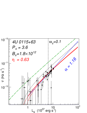
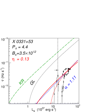
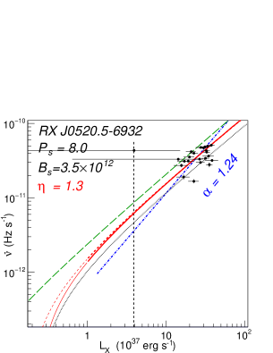
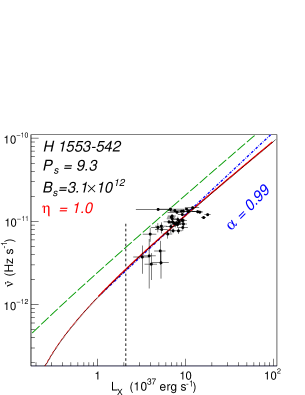
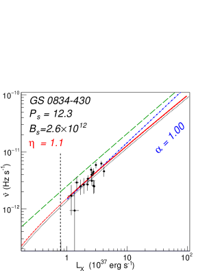
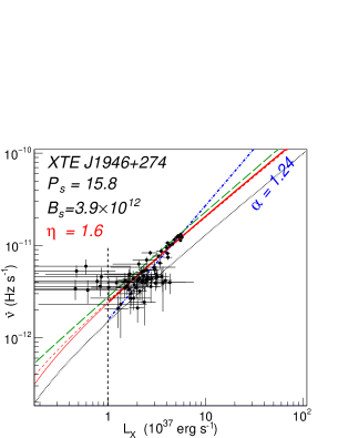
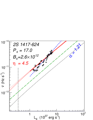
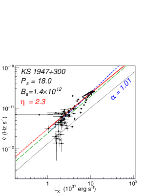
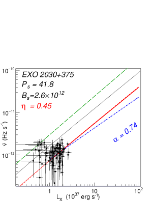
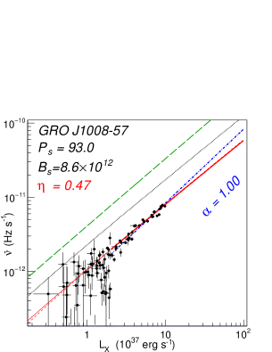
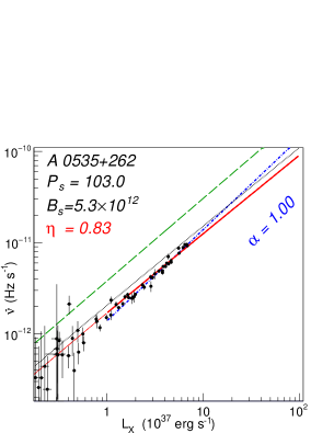
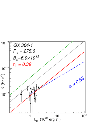
Figure 3: The $\dot{\nu}$-$L$ diagrams of the 12 Be XBPs. The best-fit power-law model is shown in a blue dash-dotted line, together with the value of $\alpha$. Black dotted and green long-dashed lines show predictions by the GL79 and the KR07 models, respectively. Thick solid and dashed lines in red are modified GL79 models in which the correction factor $\eta$ and the beaming fraction $f_{\rm b}$ are allowed to vary, respectively. The value of $L$ at $\omega_{\mathrm{s}}^{\mathrm{GL}}=0.1$ is shown by a vertical dashed line, if it is in the plot range. The spin period $P_{\rm s}$, the surface magnetic field $B_{\rm s}$ utilized in each fit, and the best-fit $\eta$ are also given in each panel.

Table 5: Summary of model fits to $\dot{\nu}_{\mathrm{s}}$-$L$ relation.

Source ID	Fitting model
	Power-law: $\dot{\nu}_{\mathrm{12}}=k\cdot L_{37}^{\alpha}$					GL79‡: $\dot{\nu}_{\mathrm{12}}=\eta\dot{\nu}^{\mathrm{GL}}(f_{\mathrm{b}}L_{37})$				KR07: $\dot{\nu}_{\mathrm{12}}=\eta\dot{\nu}^{\mathrm{KR}}$
	$k^{*}$	$\alpha^{*}$	$\xi^{\dagger}$	$\chi^{2}_{\nu}$ ($\nu$)		$\eta^{*}$ or $f_{\mathrm{b}}^{*}$	$\xi^{\dagger}$	$\chi^{2}_{\nu}$ ($\nu$)		$\eta^{*}$	$\xi^{\dagger}$	$\chi^{2}_{\nu}$ ($\nu$)
4U 0115	$0.41\pm 0.07$	$1.16\pm 0.08$	1.6	3.0 (46)		$0.632\pm 0.012$	1.6	3.1 (47)		$0.344\pm 0.007$	1.7	3.4 (47)
						$0.633\pm 0.012$	1.6	3.0 (47)
X 0331	$0.08\pm 0.04$	$1.11\pm 0.14$	5.2	35.3 (35)		$0.125\pm 0.004$	5.2	34.6 (36)		$0.070\pm 0.002$	5.2	35.0 (36)
						$0.134\pm 0.004$	5.1	32.9 (36)
RX J0520.5	$0.66\pm 0.32$	$1.24\pm 0.15$	1.6	3.4 (21)		$1.33\pm 0.06$	1.7	3.8 (22)		$0.75\pm 0.03$	1.7	3.7 (22)
						$1.37\pm 0.07$	1.7	3.8 (22)
H 1553	$1.22\pm 0.45$	$0.99\pm 0.17$	1.8	3.8 (42)		$1.01\pm 0.04$	1.8	3.8 (43)		$0.57\pm 0.02$	1.8	3.8 (43)
						$1.01\pm 0.03$	1.8	3.8 (43)
GS 0834	$1.45\pm 0.36$	$1.00\pm 0.24$	1.2	1.8 (15)		$1.11\pm 0.06$	1.1	1.7 (16)		$0.62\pm 0.03$	1.1	1.7 (16)
						$1.12\pm 0.06$	1.1	1.7 (16)
XTE J1946	$1.56\pm 0.13$	$1.24\pm 0.06$	1.0	1.0 (63)		$1.60\pm 0.02$	1.2	1.7 (64)		$0.896\pm 0.016$	1.2	1.7 (64)
						$1.66\pm 0.02$	1.2	1.7 (64)
2S 1417	$4.24\pm 0.34$	$1.21\pm 0.05$	1.6	3.2 (43)		$4.52\pm 0.04$	2.2	5.9 (44)		$2.51\pm 0.05$	2.1	5.6 (44)
						$5.52\pm 0.13$	2.3	6.4 (44)
KS 1947	$2.37\pm 0.18$	$1.01\pm 0.04$	2.4	6.6 (90)		$2.287\pm 0.016$	2.5	7.4 (91)		$1.21\pm 0.02$	2.5	7.0 (91)
						$2.59\pm 0.05$	2.6	7.5 (91)
EXO 2030	$0.79\pm 0.12$	$0.74\pm 0.28$	1.3	1.9 (68)		$0.45\pm 0.02$	1.3	1.8 (69)		$0.242\pm 0.011$	1.3	1.9 (69)
						$0.401\pm 0.014$	1.3	1.8 (69)
GRO J1008	$0.84\pm 0.07$	$1.00\pm 0.04$	2.4	7.0 (32)		$0.466\pm 0.007$	2.6	8.6 (33)		$0.245\pm 0.003$	2.5	7.8 (33)
						$0.418\pm 0.007$	2.6	8.3 (33)
A 0535	$1.38\pm 0.05$	$1.00\pm 0.02$	1.8	4.0 (32)		$0.826\pm 0.009$	2.5	7.9 (33)		$0.422\pm 0.004$	2.2	5.9 (33)
						$0.802\pm 0.004$	2.5	7.9 (33)
GX 304	$0.99\pm 0.10$	$0.63\pm 0.13$	1.6	3.5 (23)		$0.386\pm 0.015$	1.7	3.7 (24)		$0.188\pm 0.008$	1.7	3.8 (24)
						$0.332\pm 0.007$	1.7	3.7 (24)

^∗ Errors represent 1-$\sigma$ confidence limits of the fitting parameters.
^† Artificial factor to inflate the measurement errors $\Delta\dot{\nu}_{\mathrm{s}}$ and $\Delta L$ as equation (12) that can bring the model fit to the 90% confidence limit.
^‡ Top and bottom lines in each column present the results of the GL79 model fits with free-$\eta$, $f_{\mathrm{b}}=1$ and with $\eta=1$, free-$f_{\mathrm{b}}$, respectively.

Figure 4: Histograms per logarithmic intervals of the correction factor $\eta$ to the GL79 model (panel a) and to the KR07 model (panel b). In each panel, 12 arrows at the bottom indicate values for the 12 sources, and a thick arrow at the top represent the logarithmic average excluding the X 0331$+$53 data.

4 Discussion

Using the data taken by the MAXI GSC all-sky survey and the Fermi GBM pulsar project for over the 6 years since 2009 August, we analyzed the long-term X-ray intensity and pulse-period changes of the well-defined 12 Be XBPs. In all the 12 sources, the $\dot{\nu}_{\mathrm{s}}$-$L$ diagrams, obtained from large outbursts with $L\gtsim 10^{37}$ erg s^-1, show the expected positive correlations close to the direct proportionality. We performed model fits to the $\dot{\nu}_{\mathrm{s}}$-$L$ data with a power-law function and also a representative theoretical model given by GL79, leaving $\eta$ or $f_{\mathrm{b}}$ free. Below, we discuss validity of some representative theoretical models including GL79, and then consider possible origins of the scatter of $\eta$ among the sample.

4.1 Comparison among different theoretical models

4.1.1 The Ghosh & Lamb model

The $\dot{\nu}_{\mathrm{s}}$-$L$ relation of Be XBPs has been known to largely agree with the GL79 model prediction within an order of magnitude (e.g. Reynolds et al. (1996); Bildsten et al. (1997)). Through a uniform analysis of a large data sample, we improved the knowledge, in particular, the distribution of the correction factor $\eta\simeq$ 0.1–4 to the GL79 model among the 12 sources. The parameter $\eta$ is needed to bring the observed relation of each object in agreement with the GL79 model that incorporates the canonical neutron-star parameters, together with the observationally estimated $\mu$, $D$, and $f_{\mathrm{bol}}$ in equations (4), (3.4.1), (15), and (17). As obtained in section 3.4.4, the log-average of $\eta$ and its 1-$\sigma$ error among the 11 sources, excluding X 0331$+$53, are $1.0\pm 0.25$. Therefore, the GL79 model very well explains the average behavior of our sample. Because the factor $\eta$ mostly depends only on $r_{0}$, the results indicate that $r_{0}\simeq 0.5\,r_{\mathrm{a}}$ is a reasonable approximation in average. The 1-$\sigma$ range of $\eta$ given by a factor 2.1 is discussed in section 4.3.

When $L$ approaches the torque equilibrium ($\omega_{\mathrm{s}}^{\mathrm{GL}}\approx 0.35$), the $\dot{\nu}_{\mathrm{s}}$-$L$ relations of 4U 0115$+$63 and X 0331$+$53 start deviating from the direct proportionality. The GL79 model has successfully explained this important feature, behavior of 4U 1626$-$27 across the spin-up/down threshold (Takagi et al., 2016). In contrast, the other models to be considered later do not provide as successful account as GL79 of this observations.

4.1.2 The Kluźniak & Rappaport model

The success of the GL79 model in explaining the observed $\dot{\nu}_{\mathrm{s}}$-$L$ relation does not necessarily mean that the assumed physical conditions as a whole are correct. In fact, Wang (1987) and LRB95 pointed out that GL79 assume unrealistically large slip between the disk and magnetic field lines in the region between $r_{0}$ and $r_{\mathrm{a}}$. Following Wang (1987, 1995), KR07 developed alternative models in which toroidal magnetic fields are dissipated by either (A) turbulent diffusion in the disk, or (B) recombination outside the disk. Because the two KR07 assumptions lead to similar predictions, we here examine the representative one, the turbulent-disk model (A).

To visualize differences between the GL79 and KR07 models, in figure 5 we show their $\dot{\nu}_{\mathrm{s}}$-$L$ predictions, for typical values of $P_{\mathrm{s}}$ and $B_{\mathrm{s}}$, and canonical neutron-star parameters. Thus, we notice three differences between the two models.

1. In the slow-rotator regime ($\omega_{\mathrm{s}}\ll 1$), both models predict straight $\dot{\nu}_{\mathrm{s}}$-$L$ relations, but the slope is slightly different; $\alpha=0.86$ by GL97 and $\alpha=0.9$ by KR07.

2. In the same regime, the KR07 model predicts about a factor 2 higher $\dot{\nu}_{\mathrm{s}}$ than the GL79 model.

3. As $L$ decreases towards the torque equilibrium, the predictions by both models start steepening. However, this bending in KR07 takes place at a much lower luminosity ($\omega_{\mathrm{s}}\gtsim 0.9$) than in the GL79 model ($\omega_{\mathrm{s}}\sim$ 0.1).

With the above three differences in mind, we performed the KR07 model fits to the data, first without using the correction factor $\eta$. The results, presented in figure 3 in green, confirms the above property (ii). Therefore, we next incorporated $\eta$ in the same as in section 3.4.4, and obtained the fit results as summarized in table 5. (The best-fit models are not shown in figure 3 to avoid making the plots too confusing). Thus, the KR07 model with floating $\eta$ generally gave somewhat better fits to the data than the GL79 model, because of the property (i). However, the low-luminosity bending in 4U 0115$+$63 and X 0331$+$53 is better reproduced by the GL79 model, reflecting the property (iii). Furthermore, as presented in figure 4(b), the values of $\eta$ with the KR07 model became on average $\sim 0.5$ due to the property (ii), making a contrast to the GL79 result of $\langle\eta\rangle\sim 1.0$.

These comparisons, together with the success of Takagi et al. (2016), are thought to provide an a posteriori justification to our choice of GL79 as the representative accretion torque formalism.

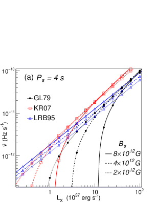
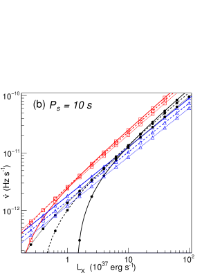
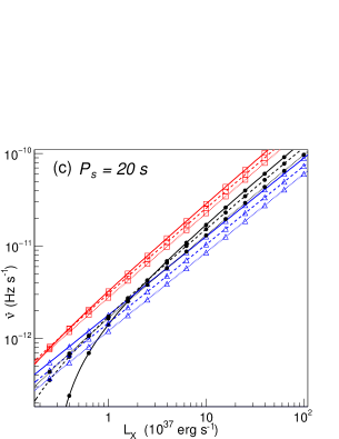
Figure 5: Theoretical $\dot{\nu}_{\mathrm{s}}$-$L$ relations in XBPs with $P_{\mathrm{s}}=$ 4 s (panel a), 10 s (panel b) , and 20 s (panel c) calculated from the GL79 (black line with dot), the KR07 (red line with triangle), and the LRB95 (blue line with box) models. Solid, dashed, and dotted lines are relations calculated for $B_{\mathrm{s}}=$ 2, 4, and 8 $\times 10^{12}$ G.

4.1.3 The Lovelace model

LRB95 developed a turbulent-disk model considering the open field lines that lead to magnetically driven outflows. It is characterized by a parameter representing the magnetic diffusivity in the disk, $\alpha_{\mathrm{m}}D_{\mathrm{m}}\simeq$ 0.01–0.1. In figure 5, the $\dot{\nu}$-$L$ relations of the LRB95 model assuming $\alpha_{\mathrm{m}}D_{\mathrm{m}}=0.1$ are plotted together with those of GL79 and KR07. In the slow-rotator regime, the LRB95 model predicts constantly $\simeq 0.7$ times smaller $\nu_{\mathrm{s}}$ than GL79. Considering that the GL79 fits gave $\langle\eta\rangle\simeq 1.0$, we need to increase the LRB95 prediction by a factor of $1/0.7$. This could be done by choosing $\alpha_{\mathrm{m}}D_{\mathrm{m}}\simeq 1$, but this falled outside its nominal range of 0.01–0.1. The model cannot either reproduce the data bending in 4U 0115$+$63 and X 0331$+$53. Yet another disadvantage of LRB95 is its failure to explain the spin-up/down transition observed from 4U 1626$-$67 (Takagi et al., 2016). Hence, we do not employ this model.

4.1.4 Other models

Campbell (2012) propose another disk-magnetosphere interaction model considering the angular-momentum feedback from the accreting matter to the disk. The model suggests that the accretion torque is reduced by a factor $\omega_{\mathrm{s}}\propto L^{-3/7}$ from that in equation (6), and thus the $\dot{\nu}_{\mathrm{s}}$-$L$ relation becomes $\dot{\nu}_{\mathrm{s}}\propto L^{3/7}$. Thus, the model is not applicable to the present data, which demand $\alpha\simeq 1$.

Motivated by an apparent double-valued $\dot{\nu}_{\mathrm{s}}$-$L$ relation observed from the slow rotator GX 304$-$1, Postnov et al. (2015) proposed a quasi-spherical accretion picture, which predicts $\alpha=7/11$ (Shakura et al., 2012). In table 5, GX 304$-$1 indeed exhibits $\alpha\simeq 0.6$ (though with the large error) in an agreement with that prediction. However, as presented in figure 3, the double-valued behavior has been explained away when using the refined orbital elements (Sugizaki et al., 2015). Therefore, it remains inconclusive whether the object prefers the model by Shakura et al. (2012).

4.2 Reconsideration of X 0331$+$53 analysis results

Among the 12 values of $\eta$ for our Be XBP sample, $\eta=0.12$ of X 0331$+$53 is unusually deviated from unity. The source also looks strange in that the estimated outburst-peak luminosity, $\sim 5\times 10^{38}$ erg s^-1, is significantly higher than those of the others ($\lesssim 10^{38}$ erg s^-1), and also exceeds the Eddington luminosity, $\simeq 2\times 10^{38}$ erg s^-1, for a $1.4M_{\odot}$ neutron star (figures 1 and 3). These facts suggest that the employed source distance, 6 kpc, from the optical photometry of the companion, BQ Cam (Reig & Fabregat, 2015), is overestimated. For example, Kodaira et al. (1985) optically estimated it as 3.5 kpc, or even smaller, just after the source was re-discovered in X-rays (Makishima et al., 1990). However, all these measurements had a problem of contaminations of infra-red emission from the Be disk (Negueruela et al., 1999; Reig & Fabregat, 2015).

In section 3.4.4, we found that the GL79 model better reproduces the X 0331$+$53 data with the bolometric correction factor $f_{\mathrm{b}}=0.12$ than with the factor $\eta=0.12$ to the $\dot{\nu}_{\mathrm{s}}$-to-$L$ coefficient. This means that the true $L$ is likely to be $\sim 0.12$ times the nominal one, and hence the actual $D$ is $6\times\sqrt{0.12}\simeq 2.4$ kpc. Considering these facts, we suggest that X 0331$+$53 is located at $D=$2–3 kpc

4.3 Estimate of physical parameter ranges

As obtained in section 3.4.4, the 1-$\sigma$ range of the correction factor $\eta$ among the 11 sources (excluding X 0331$+$53) is given by $\sigma(\log\eta)=0.31$, which means the range from $10^{-0.31}=0.49$ to $10^{0.31}=2.1$. Then, a key question is whether this scatter in $\log\eta$ can be explained by taking into account possible uncertainties in the parameters involved in the equations (4), (15), (17), and (3.4.1), or requires some corrections to the GL79 model itself. In section 4.1, we examined several alternative disk-magnetosphere models, and found that the differences among them are mostly represented by systematic differences in $\eta$. Therefore, the scatter of $\log\eta$ obtained from the 11 objects (excluding X 0331$+$53) does not depend on these models. Below, let us examine the equation for $\eta$ in a somewhat simpler form, neglecting for simplicity the general relativistic effects.

The values of $I_{45}$ are mostly determined by $M_{1.4}$ and $R_{6}$. We employed the approximating equation with them,

$$I_{45}\simeq 1.0M_{1.4}R_{6}^{2}(1-x^{-1})^{-1}\simeq 1.0M_{1.4}R_{6}^{2},$$ (19)

which is applicable to most of the major models describing the neutron-star interior (Ravenhall & Pethick, 1994).

In the GL79 model, the magnetic dipole is assumed to be aligned to the spin axis. This is however not exactly correct, because the observed X-ray fluxes are generally pulsating. Therefore, $\mu_{30}$ in equation (15) needs some corrections. At distances far from the neutron-star surface, the field strength can change by a factor of 2 according to the dipole axis orientation (Wang, 1997). We thus introduce a factor $f_{\mu}$, which takes a value from 1 to 2, and rewrite equation (17) as

$$\mu_{30}=\frac{1}{2}f_{\mu}B_{12}R_{6}^{3}\Phi(x).\simeq\frac{1}{2}bf_{\mu}E_{\mathrm{a}}R_{6}^{3},$$ (20)

where $E_{\mathrm{a}}$ refers to equation (1), and $b$ is a conversion constant in the equation.

Substituting equations (4), (19) and (20) into equation (15), we obtain

$$\dot{\nu}_{12}^{\mathrm{GL}} = 1.9\,n(\omega_{\mathrm{s}})\left(\frac{1}{2}bf_{\mu}E_{\mathrm{a}}\right)^{2/7}R_{6}^{-2/7}M_{1.4}^{-10/7}$$ (21)

$$\cdot\left(4\pi D^{2}f_{\mathrm{bol}}f_{\mathrm{b}}\right)^{6/7}C_{\mathrm{2-20}}^{6/7}$$

If the GL79 model equation (15) is accurate enough, $\eta$ will be accounted for by uncertainties or biases in the various parameters involved in equation (21). Assuming that the values of $f_{\mu}$, $E_{\mathrm{a}}$, $D$, $f_{\mathrm{bol}}$, and $f_{\mathrm{b}}$ employed above are different from their true values by factors of $10^{\pm\delta\!f_{\mu}}$, $10^{\pm\delta\!E_{\mathrm{a}}}$, $10^{\pm\delta\!D}$, $10^{\pm\delta\!f_{\mathrm{bol}}}$, and $10^{\pm\delta\!f_{\mathrm{b}}}$, respectively, we can express $\eta$ as

$$\eta = R_{6}^{-2/7}M_{1.4}^{-10/7}$$ (22)

$$\cdot({10}^{\delta\!f_{\mu}}{10}^{\delta\!E_{\mathrm{a}}})^{2/7}(10^{\delta\!f_{\mathrm{b}}}10^{\delta\!f_{\mathrm{bol}}})^{6/7}(10^{\delta\!D})^{12/7}$$

The dispersion of $\log\eta$ is then approximately reduced to

$$\sigma^{2}\left(\log\eta\right) \simeq\left(\frac{10}{7}\right)^{2}\sigma^{2}\left(\log(M_{1.4}R_{6}^{1/5})\right)$$ (23)

$$+\left(\frac{2}{7}\right)^{2}\left[\sigma^{2}\left(\delta\!f_{\mu}\right)+\sigma^{2}\left(\delta\!E_{\mathrm{a}}\right)\right]$$

$$+\left(\frac{6}{7}\right)^{2}\left[\sigma^{2}\left(\delta\!f_{\mathrm{b}}\right)+\sigma^{2}\left(\delta\!f_{\mathrm{bol}}\right)\right]$$

$$+\left(\frac{12}{7}\right)^{2}\sigma^{2}\left(\delta\!D\right),$$

where the function $\sigma^{2}()$ means the variance of a given parameter among the sample of 11 sources, and the parameter $M_{1.4}R_{6}^{1/5}$ is left as a single variable because $M$ and $R$ cannot vary independently.

In equation (23), the left-hand side shows a scatter of $\sigma(\log\eta)=0.31$ (section 3.4.4). Then, how about the right hand side ? Let us consider the involved parameters one by one.

1. As discussed above, the correction factor $f_{\mu}$ for $\mu_{30}$ is considered to take a value from 1 to 2. We hence assume $\sigma(\delta\!f_{\mu})\simeq\log 1.5=0.18$.

2. The observed CRSF energy, $E_{\mathrm{a}}$, depends on the source luminosity to some extent (section 2.3). Among the 9 sources whose CRSF has been detected in our sample, 4U 0115$+$63 exhibits the largest $E_{\mathrm{a}}$ change by 40% (e.g. Nakajima et al. (2006)). The values of $E_{\mathrm{a}}$ determined by model fits to X-ray spectra also depend on the employed model functions for the continuum and the absorption feature. However, differences among the model functions are estimated at most 10% (e.g. Mihara et al. (2004)), which is smaller than the change by the luminosity. We here employ the 1-$\sigma$ error range of 30%, and thus $\sigma(\delta\!E_{\mathrm{a}})\simeq\log 1.3=0.11$.

3. According to table 3, the 1-$\sigma$ error on $f_{\mathrm{bol}}$ is at most 10 %, which means $\sigma(\delta\!f_{\mathrm{bol}})\simeq\log 1.1=0.04$.

4. Although we have assumed $f_{\mathrm{b}}=1$ in equation (4) for simplicity, the assumption is not necessarily warranted because the source are clearly pulsating. Basko & Sunyaev (1975) suggested that it can change by a factor $\sim 2$, based on their theoretical model. Assuming that it has an 1-$\sigma$ range given by a factor 2, we obtain $\sigma(\delta\!f_{\mathrm{b}})\simeq\log 2=0.30$.

5. The errors on the source distances $D$ estimated from the optical observations are listed in table 1. They are typically $\sim 20$% although their confidence levels are not clearly given in some cases. We here assume that the 1-$\sigma$ error is $\sim 20$%, and thus $\sigma(\delta\!D)\simeq\log 1.2=0.079$

Accumulating the variances of logarithmic uncertainties in $f_{\mathrm{b}}$, $f_{\mathrm{bol}}$, $f_{\mu}$, $E_{\mathrm{a}}$, and $D$, as estimated above, and assuming that their errors are all independent from one another, the right side of equation (23) becomes

$$\sigma^{2} = \left(\frac{6}{7}\right)^{2}(0.30^{2}+0.04^{2})$$ (24)

$$+\left(\frac{2}{7}\right)^{2}(0.18^{2}+0.11^{2})$$

$$+\left(\frac{12}{7}\right)^{2}(0.079^{2})$$

$$\simeq 0.0673+0.0036+0.0183$$

$$= 0.0892\simeq 0.30^{2}.$$

The value is very close to the observed one, $\sigma^{2}(\log\eta)=0.31^{2}$. Therefore, the present high-quality data are still consistent with the GL79 model within the uncertainties considered above, and we do not need to involve a significant variance in $M_{1.4}R_{6}^{1/5}$, which has been neglected.

In equation (24), the total variance mostly owes to the two parameters, the beaming fraction $f_{\mathrm{b}}$ and the distance $D$. Further studies of these parameters will allow us to perform more accurate calibration of the GL79 formalism.

4.4 Correlations between $\eta$ and other parameters

Although we have shown that the scatter in $\eta$ can be explained by uncertainties in the involved parameters, it is still worth examining whether high-$\eta$ and low-$\eta$ XBPs have any systematic differences in their properties. For this purpose, we plot in figure 6 the two basic parameters, $P_{\mathrm{s}}$ and $B_{\mathrm{s}}$, as a function of $\eta$. In the $\eta$-$B_{\mathrm{s}}$ plot, 9 sources with secure $B_{\mathrm{s}}$ measurements were used. Figure 6 also shows the behavior of $\eta$ from the KR07 and the LRB95 models relative to the GL79 model against $P_{\mathrm{s}}$ and $B_{\mathrm{s}}$. It clearly reveals $\dot{\nu}_{\mathrm{s}}^{\mathrm{KR}}\simeq 2\dot{\nu}_{\mathrm{s}}^{\mathrm{GL}}$ and $\dot{\nu}_{\mathrm{s}}^{\mathrm{LRB}}\simeq 0.7\dot{\nu}_{\mathrm{s}}^{\mathrm{GL}}$, as discussed in section 4.1.

We observe weak negative correlations both in the $\eta$-$P_{\mathrm{s}}$ and $\eta$-$B_{\mathrm{s}}$ diagrams, in such a way that higher-field and longer-period XBPs tend to show lower $\eta$ (i.e., more difficult to be spun up). Since we already know that $P_{\mathrm{s}}$ and $B_{\mathrm{s}}$ of XBPs positively correlate with each other (e.g. Makishima et al. (1999)), the two correlations may not be independent.

One possible interpretation of figure 6 is to consider that higher-field objects with longer pulse periods may have lower values of $f_{\mathrm{b}}$, because the emission is more tightly beamed under the stronger magnetic fields, and the beam axis sweeps away from us. Yet another, more speculative possibility is to assume that higher-field objects somehow have slightly higher mass, and hence smaller values of $\eta$ via equation (22).

Even putting aside such specific causes, the negative $\eta$-$P_{\mathrm{s}}$ correlation may be explained in the following way. Some XBPs, for unspecified reasons, may intrinsically have somewhat higher values of $\eta$. Such XBPs would be more efficiently spun up by accretion, to achieve faster rotation. In contrast, those with intrinsically lower $\eta$ may end up with having long pulse periods.

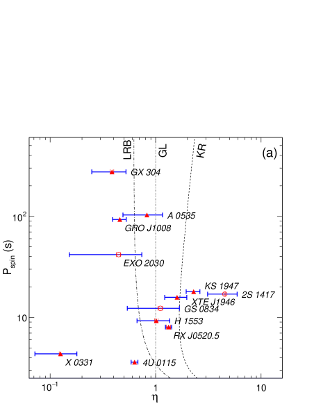
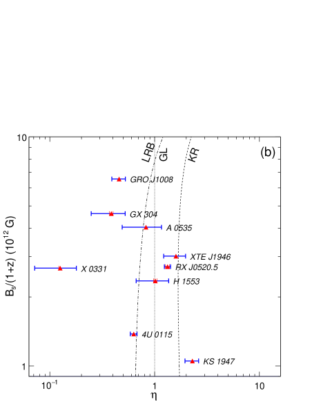
Figure 6: Distributions of $\eta$ over the 12 Be XBPs, presented versus the pulse period $P_{\mathrm{s}}$ (panel a) and the magnetic field $B_{\mathrm{s}}$ (panel b). Sources whose $B_{\mathrm{s}}$ are estimated by the CRSFs, are marked with solid triangles, and the others with open circles. Horizontal error bars in red represent the 1-$\sigma$ errors in the model fit to the $\dot{\nu}_{\mathrm{s}}$-$L$ data, and those with blue represent uncertainties expected from the errors in the parameters involved in the GL79 model formalism. Dash and dot-dash lines represent the expected behavior of $\eta$ by KR07 and LBR95, respectively, both relative to the GR79 predictions.

5 Conclusions

To examine the validity of the pulsar spin-up models due to the interaction between the pulsar magnetosphere and the accretion disk in XBPs, we analyzed the X-ray lightcurves and pulse-period variations of the 12 Be XBPs whose distance and orbital elements are well determined. The X-ray intensity was derived from the MAXI GSC data, and the timing information was derived from the Fermi GBM, both for more than 6 years since 2009. In all these objects, closely proportional relations between $\dot{\nu}_{\mathrm{s}}$ and $L$, which are expected theoretically, were confirmed. Except in X 0331$+$53, the coefficient $\eta$ of proportionality between $\dot{\nu}_{\mathrm{s}}$ and $L$ agrees, within a factor of 3, with that predicted by the GL79 model. When averaged over the 11 sources, $\eta$ becomes close to the GL79 prediction, and its scatter can be explained by uncertainties in the involved parameters, including in particular, $D$ and $f_{\mathrm{b}}$. The large discrepancy found with X 0331$+$53 is likely to arise from its distance overestimation.

The authors thank all the MAXI team members for their dedicated work on the ISS MAXI operation. Their thanks are also due to the Fermi/GBM pulsar project for providing the useful results to the public. The present work is partially supported by the Ministry of Education, Culture, Sports, Science and Technology (MEXT), Grant-in-Aid No. 25400239.

Improvements of the orbital elements

Observed pulse-period variations in XBPs include two distinct effects, the intrinsic spin-period change and the orbital Doppler shifts. In Be XBPs, both of them often correlate with the orbital phase. Therefore, it is not easy to separate the two effects from the observed period data. Actually, some of the Be XBPs analyzed here were found to show period variations coupled with the orbital modulation, even though the orbital Doppler effects had been already removed in the Fermi GBM pulsar data.

We hence construct a numerical pulse-period model, taking into account both the effects, and then fit it to the data, in an attempt to simultaneously determine the spin-period changes and improve the orbital elements. The method has been utilized in Sugizaki et al. (2015) and Marcu-Cheatham et al. (2015). The analysis procedure using the MAXI GSC and Fermi GBM data, is described below, together with the results obtained from 4U 0115$+$63, GS 0834$+$430, KS 1947$+$300, and GRO J1008$+$57.

Analysis procedure

We employed the empirical power-law model of equation (5) to express the intrinsic spin-period change. As discussed there, the frequency change during large outbursts with $L\gtsim 10^{37}$ erg s^-1 can be approximated as $\dot{\nu}_{\rm s}=kL^{\alpha}$, where $\alpha$ is $\simeq$0.85–1 and $k$ is constant. The spin frequency $\nu_{\rm s}(t)$ at a given time $t$ is then expressed by

$$\nu_{\rm s}(t)=\nu_{i}-\int_{\tau_{i}}^{t}k\left\{L(t^{\prime})\right\}^{\alpha}dt^{\prime},$$ (25)

where $\nu_{i}=\nu_{\rm s}(\tau_{i})$ are values at reference epochs $\tau_{i}$, $i=1,2..$. We defined $\tau_{i}$ for each outburst separately, because Be XBPs usually spin down gradually between the adjacent outbursts by the propeller effects.

The period modulation due to the orbital motion is calculated with the orbital elements, namely, $P_{\rm B}$, $e$, $a_{\rm x}\sin i$, $\tau_{0}$ and $\omega_{0}$ (see table 2). The velocity of the pulsar orbital motion along the line of sight, $v_{\rm l}(t)$, is represented by

$$v_{\rm l}(t)=\frac{2\pi a_{\rm x}\sin i}{P_{\rm B}\sqrt{1-e^{2}}}\left\{\cos\left(\theta(t)+\omega_{0}\right)+e\cos\omega_{0}\right\}$$ (26)

where $\theta(t)$ is a parameter called “true anomaly” associated with an elliptical orbit, and calculated from the Kepler’s equation. The observed barycentric pulse frequency, $\nu_{\rm obs}(t)$, is then expressed by

$$\nu_{\rm obs}(t)\simeq\nu_{\rm s}(t)\left(1+\frac{v_{\rm l}(t)}{c}\right)^{-1}.$$ (27)

The model represented by equations (25), (26), and (27), includes at least 7 parameters, $\nu_{0}$, $\alpha$, $k$ in (25), and 5 orbital elements in (26). We estimated the source luminosity, $L(t)$, in (26) from the GSC 2–20 keV light-curve data in 1-d time bin assuming that the emission averaged over the time bin is approximately constant and isotropic, and then fit the model to the barycentric periods from the Fermi GBM data.

In some sources, all the orbital parameters cannot be determined only from the present data. If some of the parameters are considered to be better determined in the past, we treated them as fixed ones. The details on each source are presented, in the below.

4U 0115$+$63

Figure 7 shows the fit with equations (25), (26), and (27) to the data of 4U 0115$+$63. The data are the same as in figure 1, but focused on periods of two giant outbursts. Both outbursts lasted longer than 30 d, and thus covered the entire orbital cycle of 24.3 d. We performed the period model fit by allowing all the parameters free. Thus, the fit has indeed been improved (figure 7 d) by adjusting the orbital parameters. The refined orbital parameters are listed in table 2, in comparison with the previous ones.

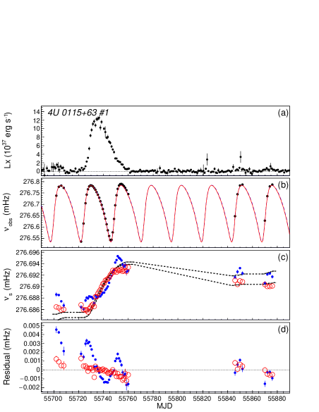
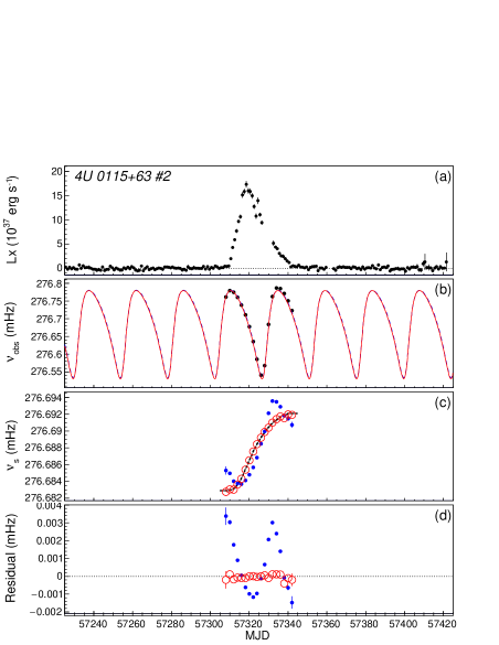
Figure 7: Model fits to the observed pulse-period evolution of 4U 0115$+$63, during the outburst in 2011 June–July (left panels) and that in 2015 October–November (right panels). (a) MAXI GSC 2-20 keV light curves. The data are the same as those in figure 1. (b) Barycentric pulse frequencies $\nu_{\mathrm{obs}}$ observed by the Fermi GBM and the expected modulation due to the orbital motion. Two modulation curves calculated from the previous orbital elements (dashed blue) in the literature and those refined in the present analysis (solid red), both of which are shown in table 2, cannot be resolved in this scale. (c) Pulsar spin frequencies $\nu_{\mathrm{s}}$ corrected for the orbital effects, employing the previous orbital elements (blue dots), and those obtained in the present analysis (red circles). A dashed line represents the best-fit spin-frequency model with equation (25). (d) Residuals of the best-fit spin frequency models, where symbols mean the same as in panel (c).

GS 0834$+$430

Figure 8 left panels present the model fit to the data of GS 0834$+$430. A significant outburst has been detected once by the two instruments, in 2012 July. The outburst lasted $\sim$ 30 d, which did not cover the entire orbital phase of 105.8 d. We thus performed the model fit with the orbital period fixed at 105.8 d, which had been obtained previously by Wilson et al. (1997), and $\alpha=6/7$. Again, the fit has been improved significantly by refining the orbital parameters. The refined parameters are listed in table 2.

KS 1947$+$300

Figure 8 right panels show the period fit for KS 1947$+$300. The source exhibited on outburst activity since 2013 September to 2015 March, where the first major outburst was followed by three minor ones. The first outburst lasted for about 100 d, which covers about two cycles of the 40.5 d orbital period. The model fit was performed by allowing all the parameters free. The data-to-model residuals at the bottom of figure 8 reveal that the artificial modulation coupled with the orbital Doppler effect has been successfully reduced.

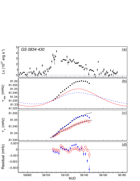
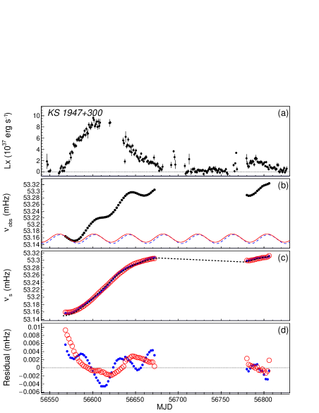
Figure 8: Model fits to observed pulse-period evolution in KS 1947$+$300 (left panels) and GS 0834$-$430 (right panels). The meanings of all symbol are same as in figure 7. In panels (b), red and blue lines represent orbital modulation calculated from the previously orbital elements and those refined in this analysis, respectively.

GRO J1008$+$57

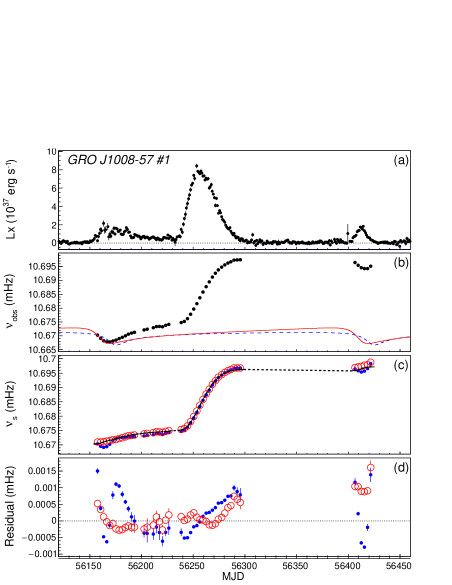
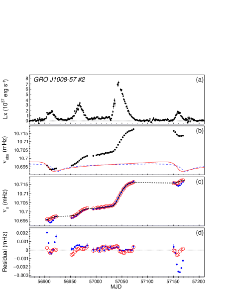
Figure 9: The same as figure 7, but for GRO J1008$-$57 in the outburst from 2012 August to 2013 January (left panels) and that from 2014 August to 2015 February (right panels).

The results on GRO J1008$+$57 are presented in figure 9, covering two extended active periods. As seen in figure 1, the source normally repeated outbursts every periastron passage by the 249.48 d orbital cycle. However, during these extended active periods, the source exhibited multiple flares almost throughout the entire orbital cycle. The orbital period is precisely determined by the pulse arrival time analysis (Kühnel et al., 2013). We thus performed the model fit with the orbital period at this value, 249.48 d. The model-fit residuals clarify that the refined orbital parameters better reproduce the observed pulse-period modulation, in particular, near the periastron phases.

References

- Arnaud (1996) Arnaud, K. A. 1996, Astronomical Data Analysis Software and Systems V, 101, 17
- Basko & Sunyaev (1975) Basko, M. M., & Sunyaev, R. A. 1975, A&A, 42, 311
- Baykal et al. (2000) Baykal, A., Stark, M. J., & Swank, J. 2000, ApJ, 544, L129
- Bildsten et al. (1997) Bildsten, L., Chakrabarty, D., Chiu, J., et al. 1997, ApJS, 113, 367
- Bonnet-Bidaud & Mouchet (1998) Bonnet-Bidaud, J. M., & Mouchet, M. 1998, A&A, 332, L9
- Bozzo et al. (2009) Bozzo, E., Stella, L., Vietri, M., & Ghosh, P. 2009, A&A, 493, 809
- Caballero et al. (2007) Caballero, I., Kretschmar, P., Santangelo, A., et al. 2007, A&A, 465, L21
- Camero-Arranz et al. (2010) Camero-Arranz, A., Finger, M. H., Ikhsanov, N. R., Wilson-Hodge, C. A., & Beklen, E. 2010, ApJ, 708, 1500
- Campbell (2012) Campbell, C. G. 2012, MNRAS, 420, 1034
- Coburn et al. (2002) Coburn, W., Heindl, W. A., Rothschild, R. E., et al. 2002, ApJ, 580, 394
- Coe et al. (1988) Coe, M. J., Payne, B. J., Longmore, A., & Hanson, C. G. 1988, MNRAS, 232, 865
- Coe et al. (1994) Coe, M. J., Roche, P., Everall, C., et al. 1994, MNRAS, 270, L57
- Coe et al. (2001) Coe, M. J., Negueruela, I., Buckley, D. A. H., Haigh, N. J., & Laycock, S. G. T. 2001, MNRAS, 324, 623
- Coe et al. (2007) Coe, M. J., Bird, A. J., Hill, A. B., et al. 2007, MNRAS, 378, 1427
- Doroshenko et al. (2016) Doroshenko, V., Tsygankov, S., & Santangelo, A. 2016, A&A, 589, A72
- Finger et al. (1996) Finger, M. H., Wilson, R. B., & Chakrabarty, D. 1996, A&AS, 120, 209
- Finger et al. (1996) Finger, M. H., Wilson, R. B., & Harmon, B. A. 1996, ApJ, 459, 288
- Finger et al. (2009) Finger, M. H., Beklen, E., Narayana Bhat, P., et al. 2009, arXiv:0912.3847
- Fürst et al. (2014) Fürst, F., et al. 2014, ApJ, 784, LL40
- Fürst et al. (2015) Fürst, F., Pottschmidt, K., Miyasaka, H., et al. 2015, ApJ, 806, L24
- Galloway et al. (2004) Galloway, D. K., at al. 2004, ApJ, 613, 1164
- Ghosh & Lamb (1979) Ghosh, P., & Lamb, F. K. 1979a, ApJ, 232, 259
- Ghosh & Lamb (1979) Ghosh, P., & Lamb, F. K. 1979b, ApJ, 234, 296
- Grindlay et al. (1984) Grindlay, J. E., Petro, L. D., & McClintock, J. E. 1984, ApJ, 276, 621
- Heindl et al. (1999) Heindl, W. A., Coburn, W., Gruber, D. E., et al. 1999, ApJ, 521, L49
- Heindl et al. (2001) Heindl, W. A., Coburn, W., Gruber, D. E., et al. 2001, ApJ, 563, L35
- İnam et al. (2004) İnam, S. Ç., Baykal, A., Matthew Scott, D., Finger, M., & Swank, J. 2004, MNRAS, 349, 173
- Israel et al. (2000) Israel, G. L., Covino, S., Campana, S., et al. 2000, MNRAS, 314, 87
- Klochkov et al. (2012) Klochkov, D., Doroshenko, V., Santangelo, A., et al. 2012, A&A, 542, L28
- Kluźniak & Rappaport (2007) Kluźniak, W., & Rappaport, S. 2007, ApJ, 671, 1990
- Kodaira et al. (1985) Kodaira, K., Nishimura, S., Kondo, M., et al. 1985, PASJ, 37, 97
- Kuehnel et al. (2014) Kuehnel, M., Finger, M. H., Fuerst, F., et al. 2014, The Astronomer’s Telegram, 5856,
- Kühnel et al. (2013) Kühnel, M., Müller, S., Kreykenbohm, I., et al. 2013, A&A, 555, A95
- Lamb et al. (1973) Lamb, F. K., Pethick, C. J., & Pines, D. 1973, ApJ, 184, 271
- Liu et al. (2006) Liu, Q. Z., van Paradijs, J., & van den Heuvel, E. P. J. 2006, A&A, 455, 1165
- Lovelace et al. (1995) Lovelace, R. V. E., Romanova, M. M., & Bisnovatyi-Kogan, G. S. 1995, MNRAS, 275, 244
- Lutovinov et al. (2016) Lutovinov, A. A., Buckley, D. A. H., Townsend, L. J., Tsygankov, S. S., & Kennea, J. 2016, MNRAS, 462, 3823
- Makishima et al. (1990) Makishima, K., Ohashi, T., Kawai, N., et al. 1990, PASJ, 42, 295
- Makishima et al. (1999) Makishima, K., Mihara, T., Nagase, F. & Tanaka, Y., 1999, ApJ, 525, 978
- Marcu-Cheatham et al. (2015) Marcu-Cheatham, D. M., Pottschmidt, K., Kühnel, M., et al. 2015, ApJ, 815, 44
- Mason et al. (1978) Mason, K. O., Murdin, P. G., Parkes, G. E., & Visvanathan, N. 1978, MNRAS, 184, 45P
- Matsuoka et al. (2009) Matsuoka, M., et al. 2009, PASJ, 61, 999
- McBride et al. (2006) McBride, V. A., Wilms, J., Coe, M. J., et al. 2006, A&A, 451, 267
- Meegan et al. (2009) Meegan, C., et al. 2009, ApJ, 702, 791
- Mihara et al. (1991) Mihara, T., Makishima, K., Kamijo, S., et al. 1991, ApJ, 379, L61
- Mihara et al. (1998) Mihara, T., Makishima, K., & Nagase, F. 1998, Advances in Space Research, 22, 987
- Mihara et al. (2004) Mihara, T., Makishima, K., & Nagase, F. 2004, ApJ, 610, 390
- Mihara et al. (2011) Mihara, T., et al. 2011, PASJ, 63, 623
- Motch & Janot-Pacheco (1987) Motch, C., & Janot-Pacheco, E. 1987, A&A, 182, L55
- Naik et al. (2013) Naik, S., Maitra, C., Jaisawal, G. K., & Paul, B. 2013, ApJ, 764, 158
- Nakahira et al. (2012) Nakahira, S., Koyama, S., Ueda, Y., et al. 2012, PASJ, 64,
- Nakajima et al. (2006) Nakajima, M., Mihara, T., Makishima, K., & Niko, H. 2006, ApJ, 646, 1125
- Nakajima et al. (2010) Nakajima, M., Mihara, T., & Makishima, K. 2010, ApJ, 710, 1755
- Negueruela et al. (1999) Negueruela, I., Roche, P., Fabregat, J., & Coe, M. J. 1999, MNRAS, 307, 695
- Negueruela & Okazaki (2001) Negueruela, I., & Okazaki, A. T. 2001, A&A, 369, 108
- Negueruela et al. (2003) Negueruela, I., Israel, G. L., Marco, A., Norton, A. J., & Speziali, R. 2003, A&A, 397, 739
- Pakull et al. (2003) Pakull, M. W., Motch, C., & Negueruela, I. 2003, The Astronomer’s Telegram, 202,
- Parkes et al. (1980) Parkes, G. E., Murdin, P. G., & Mason, K. O. 1980, MNRAS, 190, 537
- Postnov et al. (2015) Postnov, K. A., Mironov, A. I., Lutovinov, A. A., et al. 2015, MNRAS, 446, 1013
- Raichur & Paul (2010) Raichur, H., & Paul, B. 2010, MNRAS, 406, 2663
- Rappaport & Joss (1977) Rappaport, S., & Joss, P. C. 1977, Nature, 266, 683
- Ravenhall & Pethick (1994) Ravenhall, D. G., & Pethick, C. J. 1994, ApJ, 424, 846
- Reig et al. (2004) Reig, P., Negueruela, I., Fabregat, J., et al. 2004, A&A, 421, 673
- Reig et al. (2005) Reig, P., Negueruela, I., Fabregat, J., Chato, R., & Coe, M. J. 2005, A&A, 440, 1079
- Reig (2011) Reig, P. 2011, Ap&SS, 332, 1
- Reig et al. (2011) Reig, P., Nespoli, E., Fabregat, J., & Mennickent, R. E. 2011, A&A, 533, A23
- Reig & Fabregat (2015) Reig, P., & Fabregat, J. 2015, A&A, 574, A33
- Revnivtsev & Mereghetti (2015) Revnivtsev, M., & Mereghetti, S. 2015, Space Sci. Rev., 191, 293
- Reynolds et al. (1996) Reynolds, A. P., et al. 1996, A&A, 312, 872
- Riquelme et al. (2012) Riquelme, M. S., Torrejón, J. M., & Negueruela, I. 2012, A&A, 539, A114
- Santangelo et al. (1999) Santangelo, A., Segreto, A., Giarrusso, S., et al. 1999, ApJ, 523, L85
- Shakura et al. (2012) Shakura, N., Postnov, K., Kochetkova, A., & Hjalmarsdotter, L. 2012, MNRAS, 420, 216
- Shi et al. (2015) Shi, C.-S., Zhang, S.-N., & Li, X.-D. 2015, ApJ, 813, 91
- Staubert et al. (2007) Staubert, R., Shakura, N. I., Postnov, K., et al. 2007, A&A, 465, L25
- Steele et al. (1998) Steele, I. A., Negueruela, I., Coe, M. J., & Roche, P. 1998, MNRAS, 297, L5
- Sugizaki et al. (2011) Sugizaki, M. et al. 2011, PASJ, 63, 635
- Sugizaki et al. (2015) Sugizaki, M., Yamamoto, T., Mihara, T., Nakajima, M., & Makishima, K. 2015, PASJ, 67, 73
- Takagi et al. (2016) Takagi, T., Mihara, T., Sugizaki, M., Makishima, K., & Morii, M. 2016, PASJ, 68, S13
- Tendulkar et al. (2014) Tendulkar, S. P., Fürst, F., Pottschmidt, K., et al. 2014, ApJ, 795, 154
- Terada et al. (2006) Terada, Y., Mihara, T., Nakajima, M., et al. 2006, ApJ, 648, L139
- Tsygankov et al. (2012) Tsygankov, S. S., Krivonos, R. A., & Lutovinov, A. A. 2012, MNRAS, 421, 2407
- Tsygankov et al. (2016) Tsygankov, S. S., Lutovinov, A. A., Krivonos, R. A., et al. 2016, MNRAS, 457, 258
- Verrecchia et al. (2002) Verrecchia, F., Israel, G. L., Negueruela, I., et al. 2002, A&A, 393, 983
- Walter et al. (2015) Walter, R., Lutovinov, A. A., Bozzo, E., & Tsygankov, S. S. 2015, A&A Rev., 23, 2
- Wang (1987) Wang, Y.-M. 1987, A&A, 183, 257
- Wang (1995) Wang, Y.-M. 1995, ApJ, 449, L153
- Wang (1997) Wang, Y.-M. 1997, ApJ, 475, L135