Detectability of nonparametric signals: higher criticism versus likelihood ratio

Abstract

We study the signal detection problem in high dimensional noise data (possibly) containing rare and weak signals. Log-likelihood ratio (LLR) tests depend on unknown parameters, but they are needed to judge the quality of detection tests since they determine the detection regions. The popular Tukey’s higher criticism (HC) test was shown to achieve the same completely detectable region as the LLR test does for different (mainly) parametric models. We present a novel technique to prove this result for very general signal models, including even nonparametric $p$-value models. Moreover, we address the following questions which are still pending since the initial paper of Donoho and Jin: What happens on the border of the completely detectable region, the so-called detection boundary? Does HC keep its optimality there? In particular, we give a complete answer for the heteroscedastic normal mixture model. As a byproduct, we give some new insights about the LLR test’s behaviour on the detection boundary by discussing, among others, Pitmans’s asymptotic efficiency as an application of Le Cam’s theory.

and

t2Supported by DFG Grant no. 618886

1 Introduction

Signal detection in huge data sets becomes more and more important in current research. The number of relevant information is often a quite small part of the data set and hidden there. In genomics, for example, the assumption is often used that the major part of the genes in patients affected by some common diseases like cancer behaves like white noise and a minor part is differentially expressed but only slightly, see [8, 14, 20]. Consequently, the number of signals as well as the signal strength is small. This circumstance makes it difficult to decide whether there are any signals. Other application fields are disease surveillance, see [28, 32], local anomaly detection, see [33], cosmology and astronomy, see [7, 25]. In the last decade Tukey’s higher criticism (HC) test, see [35, 36, 37], modified by Donoho and Jin [11] became quite popular for these kind of problems. The reason for HC’s popularity is that the area of complete detection coincide for the HC test and the log-likelihood ratio (LLR) test under different specific model assumption, see [2, 3, 5, 6, 11, 24]. This was also done for sparse linear regression models and binary regression models, see [1, 19, 31]. To overcome the problem of an unknown noise distribution [9] used a bootstrap version of HC. A lot of related literature to the possibilities of HC, even beyond signal detection, can be found in the survey paper of [12]. For instance, [17] applied HC for classification.
There are (only) a few results concerning the asymptotic power behaviour of the LLR test on the detection boundary, which separates the area of complete detection and the area of no possible detection, see e.g. [5, 18] for the heteroscedastic and heterogeneous normal mixture models. Since [11] the questions is pending: How does HC perform on the detection boundary? Does it keep its optimality? [11] specially pointed out this question: ”Just at the critical point where r = ρ ∗ (1 + o(1)), our result says nothing; this would be an interesting (but very challenging) area for future work.”
Our paper’s purpose is twofold. First, we want to fill the theoretical gap concerning the tests’ power behaviour on the detection boundary and give an answer to the question mentioned before. We quantify the asymptotic power of the LLR test by giving the LLR statistic’s limit distribution. On the detection boundary the LLR test has nontrivial asymptotic power, whereas the HC test does not. Consequently, HC is not overall powerful. However, our message is not to scrap the idea of HC. Its power behaviour is still optimal beyond the detection boundary for a long list of models. The second purpose of our paper is to add a $p$-value model with signals coming from a nonparametric alternative to this list of models.
The paper is organized as follows. In Section 1.1 we introduce the general model and the detection testing problem. For the readers’ convenience the context and the main results are briefly illustrated for a (specific) nonparametric model in Section 1.2. The asymptotic results about the LLR test appear Section 2. Section 3 is devoted to the HC statistic and introduce an ”HC complete detection” as well as a ”trivial HC power” Theorem. Section 4 contains the application of our theory. There we discuss a generalisations of the illustrative results from Section 1.2 and the heteroscedastic normal mixture model. Although the latter was already studied in great detail we can give some new insights for it. All proofs are relegated to Appendix B

1.1 The model

Let $\{k_{n}:n\in\mathbb{N}\}\subset\mathbb{N}$, where $k_{n}\to\infty$ represents the number of observations. Throughout this paper, if not stated otherwise all limits are meant as $n\to\infty$. Let the following three mutually independent triangular arrays consisting of rowwise independent random variables are given, where values in different spaces are allowed:

• $(Z_{n,i})_{i\leq k_{n}}$ representing the noisy background, where the distribution $P_{n,i}$ of $Z_{n,i}$ is assumed to be known. In the applications we often assume that $P_{n,i}=P_{0}$ depends neither on $i$ nor on $n$, and $P_{0}$ may stand for a distribution of $p$-values under the null.

• $(X_{n,i})_{i\leq k_{n}}$ representing the signals, where the signal distribution $\mu_{n,i}$ of $X_{n,i}$ is typically unknown.

• $(B_{n,i})_{i\leq k_{n}}$ representing the appearance of a signal, where $B_{n,i}$ is Bernoulli distributed with typically unknown success probability $0\leq\varepsilon_{n,i}\leq 1$.

Instead of these random variables we observe

$$Y_{n,i}\;=\;\begin{cases}X_{n,i}&\;\textrm{ if }B_{n,i}=1\\ Z_{n,i}&\;\textrm{ if }B_{n,i}=0\\ \end{cases}$$

for all $1\leq i\leq k_{n}$. The vector $(Y_{n,1},\ldots,Y_{n,k_{n}})$ represents the noise data containing a random amount $\sum_{i=1}^{k_{n}}B_{n,i}$ of signals. It is easy to check that the distribution $Q_{n,i}$, say, of $Y_{n,i}$ is given by

(1.1) $$Q_{n,i}=(1-\varepsilon_{n,i})P_{n,i}+\varepsilon_{n,i}\mu_{n,i}=P_{n,i}+\varepsilon_{n,i}(\mu_{n,i}-P_{n,i}).$$

We are interested whether there are any signals in the noise data, i.e. whether $B_{n,i}=1$ for at least one $i=1,\ldots,k_{n}$. To be more specific, we study the testing problem

(1.2) $${\mathcal{H}}_{0,n}:\;\varepsilon_{n,i}=0\text{ for all i}\qquad\textrm{versus}\qquad{\mathcal{H}}_{1,n}:\;\varepsilon_{n,i}>0\text{ for at least one }i,$$

where we observe pure noise $(Y_{n,1},\ldots,Y_{n,k_{n}})=(X_{n,1},\ldots,X_{n,k_{n}})$ under the null. We are especially interested in the case of rare signals in the sense that

(1.3) $$\max_{1\leq i\leq k_{n}}\varepsilon_{n,i}\to 0.$$

Another typical assumption in the signal detection literature is

(1.4) $$\mu_{n,i}\ll P_{n,i}\textrm{ for all }1\leq i\leq k_{n},$$

which we also suppose throughout this paper. In Section 2.4 we discuss what happens if the assumption of absolute continuity is violated. Following the ideas of Cai and Wu [6] we explain that every model can be reduced to a model such that (1.4) is fulfilled.
Convention and Notation: Observe that

$$\frac{\,\mathrm{d}Q_{n,i}}{\,\mathrm{d}P_{n,i}}=1+\varepsilon_{n,i}\Bigl{(}\frac{\,\mathrm{d}\mu_{n,i}}{\,\mathrm{d}P_{n,i}}-1\Bigr{)}.$$

The distributions $P_{n,i},\mu_{n,i},Q_{n,i}$ and the densities $\frac{\mathrm{d}Q_{n,i}}{\,\mathrm{d}P_{n,i}}\circ pr_{i}$ shall lie on the same product space, where the projections $pr_{i}$ on the ith coordinate are suppressed throughout the paper to improve the readability. Moreover, we introduce the product measures

$$Q_{(n)}=\bigotimes_{i=1}^{k_{n}}Q_{n,i}\textrm{ and }P_{(n)}=\bigotimes_{i=1}^{k_{n}}P_{n,i}.$$

1.2 Illustration of the results and the main contents

Here, our results are briefly presented for a special nonparametric $p$-values model. For simplicity let $k_{n}=n$. Since we are dealing with $p$-values the null (noise) distribution is the uniform distribution on $(0,1)$, i.e. $P_{n,i}=P_{0}=\lambda\!\!\!\;\!\lambda_{|(0,1)}$ for all $1\leq i\leq n.$ Note that as long as the noise distribution is continuous this is not a restriction having a quantile transformation $P_{n,i}((Y_{n,i},\infty))$ or $P_{n,i}((-\infty,Y_{n,i}])$ in mind. Typically, small p-values indicates that the alternative is true, or in our case that signals are present. Respecting this we suggest signal distributions $\mu_{n,i}$ with a shrinking support $[0,\kappa_{n}]$, where

(1.5) $$\kappa_{n}=n^{-r}\textrm{ and }\varepsilon_{n,i}=\varepsilon_{n}=n^{-\beta}$$

for some $\beta\in(1/2,1)$ and $r>0$. In order to obtain such a distribution $\mu_{n,i}$ the interval $(0,\kappa_{n})$ is blown up to $(0,1)$ and a nonparametric shape function $h$ is used. Let $h:(0,1)\to(0,\infty)$ be a Lebesgue probability density, i.e. $\int_{0}^{1}h\,\mathrm{d}\lambda\!\!\!\;\!\lambda=1$, with $\int_{0}^{1}h^{2}\,\mathrm{d}\lambda\!\!\!\;\!\lambda\in(0,\infty)$ and define the signal distribution $\mu_{n,i}=\mu_{n}$ by its rescaled Lebesgue density

(1.6) $$\frac{\mathrm{d}\mu_{n}}{\,\mathrm{d}\lambda\!\!\!\;\!\lambda_{|(0,1)}}(x)=\frac{1}{\kappa_{n}}h\Bigl{(}\frac{x}{\kappa_{n}}\Bigr{)}\mathbf{1}\{x\leq\kappa_{n}\},\;x\in(0,1).$$

Since it could be to restrictive in practice to consider only measures with a shrinking support, in Section 4.1 we add a ”small” perturbation to the densities. To sum up, we have a nonparametric testing problem which can be expressed heuristically as

$$\mathcal{H}_{0,n}:\varepsilon_{n}=0\text{ versus }\mathcal{H}_{1,n}:\varepsilon>0,h\in L^{2}(P_{0})\text{ with }h\geq 0,\,\int h\mathrm{d}P_{0}=1.$$

In the following sections we give answers to the seven problems I-VII for the general model introduced in Section 1.1 and present here the corresponding results for the illustrative nonparametric $p$-value model.

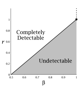
Figure 1: Left: Plot of $x\mapsto\mathrm{d}\mu_{n}/\mathrm{d}P_{0}(x)$ for $h(x)=(1-a)x^{-a}$, $a=9/20$, $r=2/3$ and $n\in\{10,25,50,100\}$, see (1.6). Right: The nonparametric detection boundary is plotted. Above the boundary is the completely detectable area and underneath is the undetectable area. The limits of the LLR statistic are Gaussian on the solid line under the null as well as under the alternative, and they are real-valued but non-Gaussian on the end of the line (solid circle). The limit under the alternative is equal to $\infty$ with a positive probability.

1. Determination of the detection boundary: Since the paper of Donoho and Jin [11] the term detection boundary is of great interest for the detection problem. This boundary splits the $r$-$\beta$ parametrisation plane into the completely detectable and the undetectable area. For each pair $(r,\beta)$ from the completely detectable area the LLR test, the optimal test, can completely separate the null and the alternative asymptotically. This means that there is a sequence $(\varphi_{n})_{n\in\mathbb{N}}$ of LLR tests with nominal levels $E_{P_{(n)}}(\varphi_{n})=\alpha_{n}$ such that $\alpha_{n}\to 0$ and the power $E_{Q_{(n)}}(\varphi_{n})$ under the alternative tends to $1$. For each $(r,\beta)$ from the undetectable area the null ${\mathcal{H}}_{0,n}$ and the alternative ${\mathcal{H}}_{1,n}$ are asymptotically indistinguishable, i.e. the sum of error probabilities tends to $1$ for each possible sequence of tests. Hence, no test yields asymptotically better results than a constant test $\varphi\equiv\alpha\in(0,1)$. For the illustrative model we have a nonparametric detection boundary which is independent of the shape function $h$ and given by

   (1.7) $$\rho(\beta)=2\beta-1\textrm{ for }\beta\in\Bigl{(}\frac{1}{2},1\Bigr{]}.$$

   The area where $r>\rho(\beta)$ ($r<\rho(\beta)$, resp.) corresponds to the completely detectable area (undetectable area, respectively), see Figure 1.

2. Gaussian limits on the detection boundary? For some parametric models the limit distribution of the log-likelihood ratio test statistic $T_{n}$, see below, was determined, e.g. for the heteroscedastic and heterogeneous normal mixture model, see Cai et al. [5] and Ingster [18]. For our model with $1/2<\beta<1$ and $r=\rho(\beta)$ we have

   $$T_{n}=\log\frac{\mathrm{d}Q_{(n)}}{\,\mathrm{d}P_{(n)}}\overset{\mathrm{d}}{\longrightarrow}\left\{\begin{array}[]{ll}\xi_{1}\sim N(-\frac{\sigma^{2}(h)}{2},\sigma^{2}(h))&\textrm{ under }{\mathcal{H}}_{0,n},\\ \xi_{2}\sim N(\phantom{-}\frac{\sigma^{2}(h)}{2},\sigma^{2}(h))&\textrm{ under }{\mathcal{H}}_{1,n},\end{array}\right.$$

   where $\sigma^{2}(h)=\int_{0}^{1}h^{2}\,\mathrm{d}\lambda\!\!\!\;\!\lambda.$ Observe that the limits only depend on the second moment of $h$ and not on its specific structure.

3. What happens if we choose the wrong $h$ or $\beta$ for the LLR statistic on the boundary? Let $(h_{1},\beta_{1})$ and $(h_{2},\beta_{2})$ represent two specific models of the illustrative example on the detection boundary, i.e. $\beta_{i}\in(1/2,1)$ and $r_{i}=\rho(\beta_{i})$ for $i=1,2$. Using Le Cam’s LAN theory we can determine the asymptotic power of the LLR test $\varphi_{n,\beta_{2},h_{2},\alpha}$ of the model $(h_{2},\beta_{2})$ of nominal level $\alpha\in(0,1)$ if $(h_{1},\beta_{1})$ is the true, underlying model:

   $$E_{\mathcal{H}_{1,n}(h_{1},\beta_{1})}(\varphi_{n,\beta_{2},h_{2},\alpha})\to\Phi\Bigl{(}u_{\alpha}+\sqrt{\sigma^{2}(h_{1})\mathrm{ARE}}\Bigr{)},$$

   $$\text{where }\mathrm{ARE}=\frac{(\int_{0}^{1}h_{1}h_{2}\,\mathrm{d}\lambda\!\!\!\;\!\lambda)^{2}}{\sigma^{2}(h_{1})\sigma^{2}(h_{2})}\mathbf{1}\{\beta_{1}=\beta_{2}\}$$

   is Pitman’s asymptotic relative efficiency, see [16], $\Phi$ denotes the distribution function of a standard normal distribution and $u_{\alpha}$ is the corresponding $\alpha$-quantile, i.e. $\Phi(u_{\alpha})=\alpha$. This formula quantifies the loss of power by choosing the wrong $\beta$ or $h$. In particular, the LLR test $\varphi_{n,\beta_{2},h_{2},\alpha}$ cannot separate the null and the alternative asymptotically, i.e ARE$=0$, if the supports of $h_{1}$ and $h_{2}$ are disjunct, or if $\beta_{1}$ and $\beta_{2}$ are unequal.

4. Beyond Gaussian limits on the detection boundary. Non-Gaussian limits of $T_{n}$ may occur, see [5, 18]. Here, such limits can be observed for $\beta=1$, $r=\rho(1)=1$. The limits are infinitely divisible distributed with nontrivial Lévy measure. These Lévy measures depend heavily on the special structure of $h$. For further results with infinitely divisible non-Gaussian $\xi_{1}$, $\xi_{2}$ confer Theorem 4.5, where we investigate in shape functions $h$ with $\int_{0}^{1}h^{2}\,\mathrm{d}\lambda\!\!\!\;\!\lambda=\infty$. Beside all this we also observe a new class of limit. To be more specific, the limit of $T_{n}$ equals $\infty$ with positive probability under the alternative, whereas the limit under the null is always real-valued (except, of course, in the completely detectable case). For $\beta=1$ and $r>1$

   $$T_{n}\overset{\mathrm{d}}{\longrightarrow}\left\{\begin{array}[]{ll}\xi_{1}\equiv-1&\textrm{ under }{\mathcal{H}}_{0,n},\\ \xi_{2}\sim e^{-1}\epsilon_{-1}+(1-e^{-1})\epsilon_{-\infty}&\textrm{ under }{\mathcal{H}}_{1,n},\end{array}\right.$$

   where $\epsilon_{a}$ denotes the Dirac measure centered in $a\in[-\infty,\infty]$, i.e. $\epsilon_{a}(A)=\mathbf{1}\{x\in A\}$. As far as we know such limits were not observed for the detection issue until now. All statements about $\beta=1$ even hold if $\int_{0}^{1}h^{2}\,\mathrm{d}\lambda\!\!\!\;\!\lambda=\infty$.

5. Extension of the detection boundary: As stated in (IV) our discussion includes $\beta=1$, whereas a lot of former research was focused (only) on $\beta<1$. The case $\beta\geq 1$ was of minor interest reason since the probability that at least one signal is present equals $1-(1-\varepsilon_{n})^{n}$, which tends to $1-e^{-1}$ and $0$ if $\beta=1$ and $\beta>1$, respectively. In particular, the pair $(\beta,r)$ with $\beta>1$ and $r>0$ always belongs to the undetectable area. Hence, $\beta>1$ do not need to be studied further. But $\beta=1$ should be taken into account, at least, when nontrivial limits are of the researcher’s interest. To sum up, the detection boundary can be extended by the case $\beta=1$, see Figure 1.

6. Optimality of HC. As already known for different mainly parametric models, we can show also for the illustrative nonparametric $p$-values model that the completely detectable regions of the LLR and the HC test coincide. By this we give a further reason why HC is a good candidate for the signal detection problem.

7. No power of HC on the boundary. We show that on the detection boundary, i.e. $\beta\in(1/2,1)$ and $r=\rho(\beta)$, the HC test cannot distinguish between the null and the alternative alternative, whereas the LLR test has nontrivial power, compare to II.

Among others, we apply our results to the model (1.6) in a more general form, e.g. $h_{n,i}$, $\kappa_{n,i}$ and $\varepsilon_{n,i}$ may depend on $i$ and $n$. We want to point out that these kind of alternatives were already studied in the context of goodness-of-fit testing by Khmaladze [26]. He used the name spike chimeric alternatives. Finally, we want to mention that our general model and the upcoming results also include

• discrete models (only for the LLR test), as the Poisson model of Arias-Castro and Wang [2].

• the sparse ($\sum_{i=1}^{k_{n}}\varepsilon_{n,i}^{2}\to 0$), the classical ($\lim_{n\to\infty}\sum_{i=1}^{k_{n}}\varepsilon_{n,i}^{2}\in(0,\infty)$) and the dense/moderately sparse case ($\sum_{i=1}^{k_{n}}\varepsilon_{n,i}^{2}\to\infty$). We used the word ”classical” for the second case corresponding heuristically to $\varepsilon_{n,i}\approx 1/\sqrt{k_{n}}$ which is the convergence rate typically used in the context of contiguous alternatives.

2 Asymptotic power behaviour of LLR tests

In this section we discuss the asymptotic power behaviour of LLR tests. These tests depend on the unknown signals and, hence, they are not applicable. But they serve as an import benchmark and all new suggested tests should be compare with the optimal LLR tests.
It is well known that at least for a subsequence $T_{n}$ converges in distribution to a random variable with values on the extended real line $[-\infty,\infty]$ under the null as well as under the alternative, see Lemma 60.6 of Strasser [34]. That is why we can assume without loss of generality that

(2.3) $$T_{n}=\sum_{i=1}^{k_{n}}\log\frac{\mathrm{d}Q_{n,i}}{\,\mathrm{d}P_{n,i}}(Y_{n,i}){\overset{\mathrm{d}}{\longrightarrow}}\left\{\begin{array}[]{ll}\xi_{1}\textrm{ under }P_{(n)}\text{ (null)},\\ \xi_{2}\textrm{ under }Q_{(n)}\text{ (alternative)},\end{array}\right.$$

where $\xi_{1}$ and $\xi_{2}$ are random variables on $[-\infty,\infty]$. Regarding the phase diagram on the right side in Figure 1 we are interested in the following three different regions/cases:

1. (Completely detectable) The LLR test $\varphi_{n}=\mathbf{1}\{T_{n}>c_{n}\}$ with appropriate critical values $c_{n}\in\mathbb{R}$ can completely separate the null and the alternative asymptotically, i.e. the sum of error probabilities $E_{\mathcal{H}_{0,n}}(\varphi_{n})+E_{\mathcal{H}_{1,n}}(1-\varphi_{n})$ tends to $0$. We will see that this corresponds to $\xi_{1}\equiv-\infty$ and $\xi_{2}\equiv\infty$.

2. (Undetectable) No test sequence $(\psi_{n})_{n\in\mathbb{N}}$ can distinguish between the null and the alternative asymptotically, i.e we always have $E_{\mathcal{H}_{0,n}}(\varphi_{n})+E_{\mathcal{H}_{1,n}}(1-\varphi_{n})\to 1$. This case corresponds to $\xi_{1}\equiv 0\equiv\xi_{2}$.

3. (Detectable) The LLR test $\varphi_{n}=\mathbf{1}\{T_{n}>c_{n}\}$ with appropriate critical values $c_{n}\in\mathbb{R}$ can separate the null and the alternative asymptotically but not completely, i.e. $E_{\mathcal{H}_{0,n}}(\varphi_{n})+E_{\mathcal{H}_{1,n}}(1-\varphi_{n})\to c\in(0,1)$.

In the following we denote the completely detectable and the undetectable case as the trivial cases since the limits of $T_{n}$ are degenerated. We start by discussing these and we present a useful tool to verify these trivial cases/limits of $T_{n}$. After that we will see that the same tools can be used to determine the nontrivial limits in the detectable case. In the last two subsections we consider the asymptotic relative efficiency, compare to (III) from Section 1.2, and explain what to do when the condition (1.4) is violated.

2.1 Trivial limits

In the proofs we work with different distances for probability measure, among others the Hellinger distance and the variational distance. Using theses distances we can classify the different detection regions. We refer the reader to the Appendix B, for further details. Here, we only present our new tool. Let us introduce for all $x>0$ the following two sums

(2.4) $$I_{n,1,x}=\sum_{i=1}^{k_{n}}\varepsilon_{n,i}\mu_{n,i}\Bigl{(}\varepsilon_{n,i}\frac{\mathrm{d}\mu_{n,i}}{\,\mathrm{d}P_{n,i}}>x\Bigr{)}$$

(2.5) and $$I_{n,2,x}=\sum_{i=1}^{k_{n}}\varepsilon_{n,i}^{2}E_{P_{n,i}}\Bigl{(}\Bigl{(}\frac{\mathrm{d}\mu_{n,i}}{\,\mathrm{d}P_{n,i}}\Bigr{)}^{2}\mathbf{1}\Bigl{\{}\varepsilon_{n,i}\frac{\mathrm{d}\mu_{n,i}}{\,\mathrm{d}P_{n,i}}\leq x\Bigr{\}}-1\Bigr{)}.$$

Theorem 2.1.

Let $\tau>0$ be fixed.

1. The completely detectable case is present if and only if $I_{n,1,\tau}$ or $I_{n,2,\tau}$ tends to $\infty$.

2. We are in the undetectable case if and only if $I_{n,1,\tau}$ as well as $I_{n,2,\tau}$ tends to $0$.

2.2 Nontrivial limits

It turns out that only a special class of distributions $\nu_{1}$ and $\nu_{2}$, say, of $\xi_{1}$ and $\xi_{2}$ may occur. The results fit in the more general framework of statistical experiments: all nontrivial weak accumulation points with respect to the weak topology of statistical experiments are infinitely divisible statistical experiments in the sense of Le Cam [29], see [30] and [23]. In the following we explain what this means in our situation. Classical infinitely divisible distributions on $(\mathbb{R},{\mathcal{B}})$ play a key role for our setting. That is why we want to recall that the characteristic function $\varphi$ of an infinitely divisible distribution on $(\mathbb{R},{\mathcal{B}})$ is given by the Lévy-Khintchine formula

$$\varphi(t)\;=\;\exp\Bigl{[}\text{i}\gamma t-\frac{\sigma^{2}t^{2}}{2}+\int_{\mathbb{R}\setminus\{0\}}\,\Bigl{(}\exp(\text{i}tx)-1-\frac{\text{i}tx}{1+x^{2}}\Bigr{)}\,\,\mathrm{d}\eta(x)\Bigr{]},\,t\in\mathbb{R},$$

where $\gamma\in\mathbb{R}$, $\sigma^{2}\in[0,\infty)$ and $\eta$ is a Lévy measure, i.e. $\eta$ is a measure on $\mathbb{R}\setminus\{0\}$ with $\int\min(x^{2},1)\,\mathrm{d}\eta<\infty$. The triple $(\gamma,\sigma^{2},\eta)$ is called the Lévy-Khintchine triple and is unique. See Gnedenko and Kolmogorov [15] for more details about infinitely divisible distributions. The following theorem gives us a characterisation of all possible limits of $T_{n}$.

Theorem 2.2.

1. Either $\xi_{1}$ is real-valued or $\xi_{1}\equiv-\infty$ with probability one. In case of the latter $\xi_{2}\equiv\infty$ with probability one.

2. Suppose $\xi_{1}$ is real-valued. Then $a=P(\xi_{2}\in\mathbb{R})>0$ and we can rewrite $\nu_{2}=a\rho+(1-a)\epsilon_{\infty}$, where $\rho(A)=a^{-1}\nu_{2}(A\cup\mathbb{R})$ for all $A\in\mathcal{B}([-\infty,\infty])$. Moreover, $\nu_{1}$ and $\rho=a^{-1}\nu_{2|\mathbb{R}}$ are infinitely divisible distributions on $(\mathbb{R},\mathcal{B})$. Let $(\gamma_{1},\sigma_{1}^{2},\eta_{1})$ and $(\gamma_{2},\sigma_{2}^{2},\eta_{2})$ be the Lévy-Khintchine triplets of $\nu_{1}$ and $\rho=a^{-1}\nu_{2|\mathbb{R}}$. Then we have:

   1. The Lévy measures $\eta_{1}$ and $\eta_{2}$ are concentrated on $(0,\infty)$, i.e. $\eta_{j}(-\infty,0)=0$. and $\int_{(0,\infty)}e^{x}\,\mathrm{d}\eta_{1}(x)<\infty$. Moreover, $\frac{\mathrm{d}\eta_{2}}{\,\mathrm{d}\eta_{1}}(x)=e^{x}\textrm{ for all }x>0.$

   2. The variances of the Gaussian parts of $\xi_{1}$ and $\xi_{2}$ coincide, i.e. $\sigma_{1}^{2}=\sigma_{2}^{2}$.

   3. The drift parameters $\gamma_{1}$ and $\gamma_{2}$ fulfill the formulas:

      (2.6) $$\log(a) =\gamma_{1}+\frac{\sigma^{2}_{1}}{2}-\int_{(0,\infty)}\Bigl{(}1-e^{x}+\frac{x}{1+x^{2}}\Bigr{)}\>\,\mathrm{d}\eta_{1}(x),$$

      (2.7) $$\gamma_{2} =\gamma_{1}+\sigma^{2}_{1}+\int_{(0,\infty)}(e^{x}-1)\frac{x}{1+x^{2}}\,\mathrm{d}\eta_{1}(x).$$

Remark 2.3.

If $\xi_{1}$ is real-valued then by Le Cam’s first Lemma the null (product) measure $P_{(n)}$ is contiguous with respect to the alternative (product) measure $Q_{(n)}$, i.e. $Q_{(n)}(A_{n})\to 0$ implies $P_{(n)}(A_{n})\to 0$. If additionally $\xi_{2}$ is real-valued then $P_{(n)}$ and $Q_{(n)}$ are mutually contiguous, i.e. $Q_{(n)}(A_{n})\to 0$ if and only if $P_{(n)}(A_{n})\to 0$. Observe that under mutually contiguity a random variable is asymptotically constant under the null $P_{(n)}$ if and only if this is the case under the alternative $Q_{(n)}$.

According to Theorem 2.2(b) the Lévy-Khintchine triplets of $\nu$ and $\rho=a^{-1}\nu_{2|\mathbb{R}}$ are closely related to each other. This was already observed in the context of statistical experiments by Janssen et al. [22].
Now, we know the class of all possible limits and, hence, the questions arises naturally how to determine the distribution of $\xi_{1}$ and $\xi_{2}$ for a given setting. To answer this question we first observe that by Theorem 2.2(bi) the Lévy measures $\eta_{1}$ and $\eta_{2}$ are uniquely determined by their difference $M=\eta_{2}-\eta_{1}$. Combining this, Theorem 2.2(bii) and Theorem 2.2(biii) yields that $M$, $\sigma_{1}^{2}$ and $a=\nu_{2}(\mathbb{R})$ serve to understand the distribution of $\xi_{1}$ and $\xi_{2}$ completely. We will see that these three are determined by the limits of the sums given by (2.4) and (2.5). To give a first impression why this is the case we explain briefly the impact of $I_{n,1,x}$. Since the summands of $T_{n}$ fulfill the so-called condition of infinite smallness, i.e. a finite number of summands has no influence of the sum’s convergence behaviour, well-known limit theorems to infinitely divisible distributed random variable can be applied, see, for instance, Gnedenko and Kolmogorov [15]. In the case of real-valued $\xi_{1}$ we obtain from these theorems

(2.8) $$\sum_{i=1}^{k_{n}}P_{n,i}\Bigl{(}\varepsilon_{n,i}\frac{\mathrm{d}\mu_{n,i}}{\,\mathrm{d}P_{n,i}}>e^{x}-1+\varepsilon_{n,i}\Bigr{)}\to\eta_{1}(x,\infty)$$

for all x from a dense subset of $(0,\infty)$. If additionally $\xi_{2}$ is real valued then the same holds for $\eta_{2}$ when we replace $P_{n,i}$ by $Q_{n,i}$. Combining these and (1.3) shows that $I_{n,1,e^{x}-1}$ tends to $M(x,\infty)=(\eta_{2}-\eta_{1})(x,\infty)$ for all x coming from a dense subset of $(0,\infty)$ if both, $\xi_{1}$ and $\xi_{2}$, are real-valued. In the case of $a=\nu_{2}(\mathbb{R})=P(\xi_{2}\in\mathbb{R})<1$ a similar convergence can be observed, namely $I_{n,1,e^{x}-1}$ tends to $(\eta_{2}-\eta_{1})(x,\infty)+M(\infty)$, where the mass $M(\infty)$ in the point $\infty$ characterizes $a$ uniquely.

Theorem 2.4.

Let $I_{n,1,x}$ and $I_{n,2,x}$, $x>0$, be defined as in (2.4) and (2.5). $\xi_{1}$ is real-valued if and only if the following (a) and (b) hold:

1. There is a dense subset ${\mathcal{D}}$ of $(0,\infty)$ and a measure $M$ on $((0,\infty],{\mathcal{B}}(0,\infty])$ such that for all $x\in{\mathcal{D}}$

   $$\lim_{n\to\infty}I_{n,1,e^{x}-1}=M(x,\infty].$$

2. For some $\sigma^{2}\in[0,\infty)$ we have

   $$\lim_{x\searrow 0}\,\underset{n\to\infty}{\begin{subarray}{c}\limsup\\ \liminf\end{subarray}}\;I_{n,2,x}=\sigma^{2},$$

   i.e. this equation holds for $\limsup_{n\to\infty}$ and $\liminf_{n\to\infty}$ simultaneously.

If (a) and (b) hold then using the notation from Theorem 2.2(b) we obtain $\nu_{2}(\mathbb{R})=\exp(-M(\{\infty\})),$ $\sigma^{2}=\sigma_{1}^{2}=\sigma_{2}^{2}$ and $\eta_{2}-\eta_{1}=M_{|(0,\infty)}$.

Remark 2.5.

1. From Theorem 2.2(bi) we get for all $x>0$

   (2.9) $$\frac{\mathrm{d}\eta_{1}}{\,\mathrm{d}M}(x)=\frac{1}{\exp(x)-1}\textrm{ and }\frac{\mathrm{d}\eta_{2}}{\,\mathrm{d}M}(x)=\frac{\exp(x)}{\exp(x)-1}.$$

2. Consider the rowwise identical case with a noise distribution independent on $n$, i.e. $P_{n,i}=P_{0}$, $\mu_{n,i}=\mu_{n}$ and $\varepsilon_{n,i}=\varepsilon_{n}$. Thus, $Y_{n,1},\ldots,Y_{n,k_{n}}$ are identical $P_{0}$-distributed under the null. By using techniques of extreme value theory it is sometimes possible to show that

   $$\max_{1\leq i\leq k_{n}}\Bigl{\{}\varepsilon_{n}\frac{\mathrm{d}\mu_{n}}{\,\mathrm{d}P_{0}}(Y_{n,i})\Bigr{\}}\overset{\mathrm{d}}{\longrightarrow}\widetilde{Y}$$

   for a real-valued random variable $\widetilde{Y}$. Note that $\max_{1\leq i\leq k_{n}}\{P_{n,i}(\varepsilon_{n,i}\frac{\mathrm{d}\mu_{n,i}}{\,\mathrm{d}P_{n,i}}>\tau)\}\leq\tau^{-1}\max_{1\leq i\leq k_{n}}\varepsilon_{n,i}\to 0$. Hence, regarding (2.8) we get the following connection to the Lévy measure $\eta_{1}$ of $\xi_{1}$:

   $$P(Y>e^{x}-1)=\exp(-\eta_{1}(x,\infty))$$

   for all $x$ coming from a dense subset of $(0,\infty)$. This may be useful to get a first impression how to choose $\mu_{n}$ and $\varepsilon_{n}$ to obtain nontrivial limits.

2.3 Asymptotic relative efficiency

In the case of normal distributed limits we have

(2.12) $$T_{n}{\overset{\mathrm{d}}{\longrightarrow}}\left\{\begin{array}[]{ll}\xi_{1}\sim N(-\sigma^{2}/2,\sigma^{2})\textrm{ under }P_{(n)}\text{ (null)},\\ \xi_{2}\sim N(\sigma^{2}/2,\sigma^{2})\textrm{ under }Q_{(n)}\text{ (alternative)},\end{array}\right.$$

for some $\sigma\in[0,\infty)$, where $N(0,0)$ denotes the Dirac measure $\epsilon_{0}$ centered in $0$. In the case of $\sigma=0$ no test sequence can separate between the null and the alternative asymptotically, see Section 2.1. Observe that both normal distributed limits depend only on one parameter, namely $\sigma^{2}$. In Appendix A, see Theorem A.1, we give many different equivalent conditions for normal distributed $\xi_{1}$ and $\xi_{2}$, even the conditions in Theorem 2.2 can be simplified in this case. Further equivalent conditions and closely related results can be found in Section A3 and A4 of Janssen [23]. In this section we restrict ourselves to these kind of limits, excluding the trivial case $\sigma=0$, and discuss the LLR test’s power behaviour if the ”wrong” signal distributions and/or the ”wrong” signal probabilities are chosen for the test statistic. To be more specific, we fix the triangular schemes of noise distributions $\{P_{n,i}:1\leq i\leq n\in\mathbb{N}\}$ and consider for $j=1,2$ a triangular scheme of signal distributions $\boldsymbol{\mu^{(j)}}=\{\mu_{n,i}^{(j)}:1\leq i\leq n\in\mathbb{N}\}$ as well as one of signal probabilities $\boldsymbol{\varepsilon^{(j)}}=\{\varepsilon_{n,i}^{(j)}:1\leq i\leq n\in\mathbb{N}\}$. Let $\boldsymbol{\theta_{1}}=(\boldsymbol{\mu^{(1)}},\boldsymbol{\varepsilon^{(1)}})$ be the true, underlying model and $\boldsymbol{\theta_{2}}=(\boldsymbol{\mu^{(2)}},\boldsymbol{\varepsilon^{(2)}})$ be the model pre-chosen by the statistician for the LLR test. Denote by $T_{n}(\boldsymbol{\theta_{j}})$ and $\varphi_{n}(\boldsymbol{\theta_{j}})=\mathbf{1}\{T_{n}(\boldsymbol{\theta}_{j})>c_{n,j}\}$ the LLR statistic and the LLR test for the model $\boldsymbol{\theta_{j}}$, $j=1,2$. Using Pitman’s asymptotic relative efficiency, see Hájek et al. [16], we quantify the loss in terms of the asymptotic power if $\varphi_{n}(\boldsymbol{\theta_{2}})$ instead of the optimal $\varphi_{n}(\boldsymbol{\theta_{1}})$ is used.

Theorem 2.6 (LLR power under Gaussian limits).

Suppose that $T_{n}(\boldsymbol{\theta_{j}})$, $j\in\{1,2\}$, converges to Gaussian limits, compare to (2.12), with $\sigma_{j}>0$. Moreover, assume that for $j,m\in\{1,2\}$ the limit

(2.13) $$\gamma(\boldsymbol{\theta_{j}},\boldsymbol{\theta_{r}})=\lim_{n\to\infty}\sum_{i=1}^{k_{n}}\varepsilon^{(j)}_{n,i}\varepsilon_{n,i}^{(r)}\text{Cov}_{P_{n,i}}\Bigl{(}\frac{\mathrm{d}\mu_{n,i}^{(j)}}{\,\mathrm{d}P_{n,i}},\frac{\mathrm{d}\mu_{n,i}^{(r)}}{\,\mathrm{d}P_{n,i}}\Bigr{)}$$

exists in $\mathbb{R}$. Suppose that $\gamma(\boldsymbol{\theta_{j}},\boldsymbol{\theta_{j}})=\sigma_{j}^{2}$. Let the critical values $c_{n,j}$ be chosen such that both tests $\varphi_{n}(\boldsymbol{\theta_{1}})$ and $\varphi_{n}(\boldsymbol{\theta_{2}})$ are asymptotically exact of a pre-chosen size $\alpha\in(0,1)$, i.e. $E_{\mathcal{H}_{0,n}}(\varphi_{n}(\boldsymbol{\theta_{1}}))\to\alpha$. Then the asymptotic power of the pre-chosen LLR test $\varphi_{n}(\boldsymbol{\theta_{2}})$ under the alternative ${\mathcal{H}}_{1,n}(\boldsymbol{\theta_{1}})$ of the true, underlying model $\boldsymbol{\theta_{1}}$ is given by

$$E_{{\mathcal{H}}_{1,n}(\boldsymbol{\theta_{1}})}(\varphi_{n,\boldsymbol{\theta_{2}}}) \to\Phi\Bigl{(}\frac{\gamma(\boldsymbol{\theta_{1}},\boldsymbol{\theta_{2}})}{\sqrt{\gamma(\boldsymbol{\theta_{2}},\boldsymbol{\theta_{2}})}}+u_{\alpha}\Bigr{)}$$

$$=\Phi\Bigl{(}\mathrm{sign}(\gamma(\boldsymbol{\theta_{1}},\boldsymbol{\theta_{2}}))\sqrt{\gamma(\boldsymbol{\theta_{1}},\boldsymbol{\theta_{1}})\mathrm{ARE}}+u_{\alpha}\Bigr{)},$$

$$\text{where }\mathrm{ARE}=\frac{\gamma(\boldsymbol{\theta_{1}},\boldsymbol{\theta_{2}})^{2}}{\gamma(\boldsymbol{\theta_{1}},\boldsymbol{\theta_{1}})\gamma(\boldsymbol{\theta_{2}},\boldsymbol{\theta_{2}})}\in[0,1]$$

is Pitman’s asymptotic relative efficiency, see Hájek et al. [16].

Remark 2.7.

The assumption $\gamma(\boldsymbol{\theta_{j}},\boldsymbol{\theta_{j}})=\sigma_{j}^{2}$ is connected to the classical Lindeberg-condition. It is often but not always fulfilled if (2.12) holds. For example, it is violated in the case $\beta=3/4$ and $r=\rho(\beta)$ for the heterogeneous normal mixture model, which is discussed in Section 4.2. The good news are that by a truncation argument we find for every model $\boldsymbol{\theta}=(\boldsymbol{\mu},\boldsymbol{\varepsilon})$, for which (2.12) holds, another $\boldsymbol{\widetilde{\theta}}=(\boldsymbol{\widetilde{\mu}},\boldsymbol{\widetilde{\varepsilon}})$ such that the limit $\gamma(\boldsymbol{\widetilde{\theta}},\boldsymbol{\widetilde{\theta}})$ from (2.13) exists and equals $\sigma^{2}$ from (2.12), and, moreover, the test’s asymptotic behaviour is not effected by replacing $\boldsymbol{\theta}$ by $\boldsymbol{\widetilde{\theta}}$. The details are carried out in Appendix A, see Lemma A.3.

Note that Theorem 2.6 gives the sharp upper bound of the asymptotic power for all tests of asymptotic size $\alpha\in(0,1)$ if (2.12) holds for the underlying model. The asymptotic relative efficiency ARE is a good tool to quantify the loss of power if the wrong LLR test is used. If $\mathrm{ARE}=1$ there is no loss of power by using $\varphi_{n}(\boldsymbol{\theta_{2}})$ and if $\mathrm{ARE}=0$ the test $\varphi_{n}(\boldsymbol{\theta_{2}})$ cannot distinguish between the null and the alternative asymptotically. Consider for a moment the rowwise identical case, i.e. $P_{n,i}=P_{n,1}$, $\mu^{(1)}_{n,i}=\mu_{n,1}^{(1)}$ etc. If $\mathrm{ARE}\in(0,1)$ then, heuristically, $(1-\mathrm{ARE})\cdot 100\%$ of the observations are wasted. To be more specific, it can be shown that $\varphi_{n}(\boldsymbol{\theta}_{2})$ based on all $k_{n}$ observations $(Y_{n,1},\ldots,Y_{n,k_{n}})$ achieves the same power as the optimal test does when only $m=[(1-ARE)k_{n}]$ observations $(Y_{n,1},\ldots,Y_{n,m})$ are used, where $[x]$ is the integer part of $x\in\mathbb{R}$.

2.4 Violation of (1.4)

Here, we discuss how to handle a violation of (1.4). This issue was already discussed by Cai and Wu [6], see their Section III.C, in terms of the Hellinger distance to determine the detection boundary. Their idea can be used for our purpose to determine, more generally, the limits of $T_{n}$, even on the boundary. Instead of the original model it is sufficient to analyse a ”closely related” model for which (1.4) is fulfilled.
By Lebesgues’ decomposition, see Lemma 1.1 of Strasser [34], there exist a constant $\kappa_{n,i}\in[0,1]$, a $P_{n,i}$-null set $N_{n,i}$ as well as probability measures $\widetilde{\mu}_{n,i}$ and $\nu_{n,i}$ such that $\widetilde{\mu}_{n,i}\ll P_{n,i},$ $\nu_{n,i}(N_{n,i})=1$ and $\mu_{n,i}=(1-\kappa_{n,i})\widetilde{\mu}_{n,i}+\kappa_{n,i}\nu_{n,i}$. Now, let $\widetilde{Q}_{n,i}$, $\widetilde{Q}_{(n)}$ and $\widetilde{T}_{n}$ defined as $Q_{n,i}$, $Q_{(n)}$ and $T_{n}$ replacing $\mu_{n,i}$ and $\varepsilon_{n,i}$ by $\widetilde{\mu}_{n,i}$ and $\widetilde{\varepsilon}_{n,i}$, respectively. Clearly, for this new model (1.4) is fulfilled and our results can be applied to determine the limits of $\widetilde{T}_{n}$. When knowing these we can immediately give the ones of $T_{n}$:

Corollary 2.8.

Suppose that (2.3) is fulfilled for $\widetilde{T}_{n}$, $\widetilde{\xi}_{1}$ and $\widetilde{\xi}_{2}$. Moreover, assume that $\sum_{i=1}^{k_{n}}\varepsilon_{n,i}\kappa_{n,i}\to c\in[0,\infty]$. Then (2.3) holds for $T_{n}$, $\xi_{1}=\widetilde{\xi}_{1}-c$ and $\xi_{2}=\widetilde{\xi}_{2}+X$, where $X$ is independent of $\widetilde{\xi}_{2}$ with $P(X=-c)=e^{-c}$ and $P(X=\infty)=1-e^{-c}$. In particular, $\xi_{1}\equiv-\infty$ and $\xi_{2}\equiv\infty$ if $c=\infty$, or if $\widetilde{\xi}_{1}\equiv-\infty$ and $\widetilde{\xi}_{2}\equiv\infty$.

We can state the results of Corollary 2.8 also in terms of distributions. Denote by $\widetilde{\nu}_{j}$ the distribution of $\widetilde{\xi}_{j}$. Then $\nu_{1}=\widetilde{\nu}_{1}*\epsilon_{-c}$ and $\nu_{2}=e^{-c}\widetilde{\nu}_{2}*\epsilon_{-c}+(1-e^{-c})\epsilon_{\infty}$.

3 Power of the higher criticism test

In the previous section we discussed the LLR test which can be used to detect simple alternatives from the null. An adaptive and applicable test for alternatives of the whole completely detectable area is Tukey’s HC test modified by Donoho and Jin [11]. There are different versions of it. We prefer the one dealing with continuously distributed $p$-values $(p_{n,i})_{i\leq k_{n}}$ and consider $P_{n,i}=\lambda\!\!\!\;\!\lambda_{|(0,1)}$ having a quantile transformation $p_{n,i}=P_{n,i}((Y_{n,i},\infty))$ or $p_{n,i}=P_{n,i}((-\infty,Y_{n,i}])$ in mind. The optimality of HC in a discrete model, namely the Poisson means model, was shown by Arias-Castro and Wang [2]. Our results about the LLR statistic in Section 2 are valid for discrete models but in this section we only regard continuous ones. The extension to discrete models is a possible project for the future.
The HC statistic for outcomes $p_{n,i}\in[0,1]$ is defined by

$$HC_{n}=\sup_{t\in(0,1)}\Bigl{|}\sqrt{k_{n}}\;\frac{\mathbb{F}_{n}(t)-t}{\sqrt{t(1-t)}}\Bigr{|},$$

where $\mathbb{F}_{n}$ is the empirical distribution function of the observation vector $(p_{n,i})_{i\leq k_{n}}$. For every $t\in(0,1)$ we compare the empirical distribution function and the null/noise distribution function $t\mapsto F(t)=t$. This difference is normalized in the spirit of the central limit theorem. For a fixed $t$ the resulting fraction is asymptotically standard normal distributed. The interval $(0,1)$, over which the supremum is taken, can be replaced by $(0,\alpha_{0})$, $(k_{n}^{-1},\alpha_{0})$ or $(k_{n}^{-1},1-k_{n}^{-1})$ for some tuning parameter $\alpha_{0}\in(0,1)$, see Donoho and Jin [11]. The test statistic can also be defined without taking the absolute value of the fraction. All these versions of the HC statistic would lead here to the same power results. To improve the readability of this section we give the results only for the HC version introduced above. By Jaeschke [21], see also Eicker [13], the limit distribution of $HC_{n}$ is known under the null. We have

(3.1) $$P_{(n)}(a_{n}HC_{n}-b_{n}\leq x)\to\Lambda(x)^{2}=\exp(-2\exp(-x)),\;x\in\mathbb{R},$$

where $\Lambda$ is the distribution function of a standard Gumbel distribution and the following normalisation constants are used

$$a_{n}=\sqrt{2\log\log(k_{n})}\textrm{ and }b_{n}=2\log\log(k_{n})+\frac{1}{2}\log\log\log(k_{n})-\frac{1}{2}\log(\pi).$$

Hence, the test $\varphi_{n,HC,\alpha}=\mathbf{1}\{HC_{n}>c_{n}(\alpha)\}$ with

$$c_{n}(\alpha)=\frac{-\log(-\log(\alpha)/2)+b_{n}}{a_{n}}=\sqrt{2\log\log(k_{n})}(1+o(1))$$

is an asymptotically exact level $\alpha\in(0,1)$ test, i.e. $E_{\mathcal{H}_{0,n}}(\varphi_{n,HC,\alpha})\to\alpha$. But we cannot recommend to use these critical values based on the limiting distribution since the convergence rate is really slow, see Khmaladze and Shinjikashvili [27]. Since the noise distribution is known, standard Monte-Carlo simulations can be used to estimate the $\alpha$-quantile of $HC_{n}$ for finite sample size. Alternatively, you can find finite recursion formulas for the exact finite distribution in the paper of Khmaladze and Shinjikashvili [27].
In the following we present our tool for HC.

Theorem 3.1 (Completely detectable by HC).

Define for all $v\in(0,1/2)$

(3.2) $$H_{n}(v)=\frac{|\sum_{i=1}^{k_{n}}\varepsilon_{n,i}(\mu_{n,i}(0,v]-v)|+|\sum_{i=1}^{k_{n}}\varepsilon_{n,i}(\mu_{n,i}(1-v,1)-v)|}{\sqrt{k_{n}v}}.$$

Let $(v_{n})_{n\in\mathbb{N}}$ be a sequence in the interval $(0,1/2)$ such that $a_{n}^{-1}H_{n}(v_{n})\to\infty$ and $\liminf_{n\to\infty}k_{n}v_{n}>0$. Then $a_{n}HC_{n}-b_{n}\to\infty$ in $Q_{(n)}$-probability.

Basically, we compare the tails near to $0$ and $1$ of the signal and the noise distribution. This verification method for HC’s optimality is an extension of the ones used by [5, 11]. Under the assumptions of Theorem 3.1 the sum of HC’s error probabilities tends to $0$ for appropriate critical values. In other words, HC can completely separate the null and the alternative.
The same $H_{n}(v)$ can be used to show that HC has no power under the alternative, i.e. the sum of error probabilities tends to $1$ independently how the critical values are chosen.

Theorem 3.2 (Undetectable by HC).

Suppose that $P_{n,i}=P_{n}$, $\varepsilon_{n,i}=\varepsilon_{n}$ and $\mu_{n,i}=\mu_{n}$ do not depend on $i$. Define $H_{n}(v)$ as in Theorem 3.1. Moreover, assume that $P_{(n)}$ and $Q_{(n)}$ are mutually contiguous, compare to Remark 2.3. If

(3.3) $$a_{n}\sup\{H_{n}(v):v\in[r_{n},s_{n}]\cup[t_{n},u_{n}]\}\to 0,\textrm{ where }$$

(3.4) $$\frac{\log(r_{n})}{\log(k_{n})}\to-1,\;\frac{\log(u_{n})}{\log(k_{n})}\to 0,\;\textrm{ and }\;\frac{\log(s_{n})}{\log(k_{n})},\frac{\log(t_{n})}{\log(k_{n})}\to\kappa\in(0,1)$$

for some sequences $r_{n},s_{n},t_{n},u_{n}\in(0,1)$ then

(3.5) $$Q_{(n)}(a_{n}HC_{n}-b_{n}\leq x)\to\Lambda(x)^{2}=\exp(-2\exp(-x)),\;x\in\mathbb{R}.$$

Remark 3.3.

Suppose that $a_{n}^{2}\sum_{i=1}^{k_{n}}\varepsilon_{n,i}^{2}\to 0$, which is usually fulfilled for sparse signals. From Hölder’s inequality $(a_{n}/\sqrt{k_{n}})\sum_{i=1}^{k_{n}}\varepsilon_{n,i}\to 0$ follows. Hence, it is easy to see that the statements of Theorems 3.1 and 3.2 remain true if $H_{n}(v)$ is replaced by

$$\widetilde{H}_{n}(v)=\frac{1}{\sqrt{k_{n}v_{n}}}\Bigl{(}\sum_{i=1}^{k_{n}}\varepsilon_{n,i}(\mu_{n,i}(0,v]+\mu_{n,i}(1-v,1))\Bigr{)},\;v\in\Bigl{(}0,\frac{1}{2}\Bigr{)}.$$

4 Application to practical detection models

4.1 Nonparametric alternatives for $p$-values

Here, we discuss a generalisation of the $p$-values model (1.6). In particular, we suppose $P_{n,i}=\lambda\!\!\!\;\!\lambda_{|(0,1)}$. In contrast to Section 1.2, we now consider that the shape function $h_{n,i}$, the shrinking parameter $\kappa_{n,i}>0$ and the signal probability $\varepsilon_{n,i}$ may depend on $i$. The assumption that the signal distribution has a shrinking support can be too restrictive for practice. But the approach allows an extension of the model in the way that we add a perturbation $r_{n,i}$. Throughout this section we consider signal distributions $\mu_{n,i}$ given by

(4.1) $$\frac{\mathrm{d}\widetilde{\mu}_{n,i}}{\,\mathrm{d}\lambda\!\!\!\;\!\lambda_{|(0,1)}}(u)=\frac{1}{\kappa_{n,i}}h_{n,i}\Bigl{(}\frac{u}{\kappa_{n,i}}\Bigr{)}+r_{n,i}(u)\geq 0\textrm{ with }\int_{0}^{1}r_{n,i}\,\mathrm{d}\lambda\!\!\!\;\!\lambda=0,$$

where $h_{n,i}$ is close to some $h\in L^{1}(\lambda\!\!\!\;\!\lambda_{|(0,1)})$ and the perturbation $r_{n,i}$ is ”small” in the sense that

(4.2) $$\sum_{i=1}^{k_{n}}\varepsilon_{n,i}^{2}\int_{0}^{1}r_{n,i}^{2}\,\mathrm{d}\lambda\!\!\!\;\!\lambda\to 0.$$

Instead of (1.5) we suppose that

$$\max_{1\leq i\leq k_{n}}(\varepsilon_{n,i}+\kappa_{n,i})\to 0.$$

Since we already presented the results concerning this model for the rowwise identical case $\mu_{n,i}=\mu_{n}$ and $\varepsilon_{n,i}=\varepsilon_{n}$ in Section 1.2, the theorems are stated only in their general versions here.

Theorem 4.1.

Suppose that

(4.3) $$\sum_{i=1}^{k_{n}}\frac{\varepsilon_{n,i}^{2}}{\kappa_{n,i}}\to K\in[0,\infty]\textrm{ and }\max_{1\leq i\leq k_{n}}\int_{0}^{1}(h_{n,i}-h)^{2}\,\mathrm{d}\lambda\!\!\!\;\!\lambda\to 0$$

for some $h,h_{n,i}\in L^{2}(\lambda\!\!\!\;\!\lambda_{|(0,1)})$. Without loss of generality we can suppose that

$$\frac{\varepsilon_{n,1}}{\kappa_{n,1}}\leq\frac{\varepsilon_{n,2}}{\kappa_{n,2}}\leq\ldots\leq\frac{\varepsilon_{n,k_{n}}}{\kappa_{n,k_{n}}}.$$

1. (Undetectable case) If $K=0$ then the undetectable case is present.

2. (Completely detectable case) If $K=\infty$,

   (4.4) $$\sum_{i=r_{n}}^{k_{n}}\varepsilon_{n,i}\to\infty\textrm{ and }\sum_{i=1}^{r_{n}}\frac{\varepsilon_{n,i}^{2}}{\kappa_{n,i}}\to\infty.$$

   for some $r_{n}\in\{1,\ldots,k_{n}\}$ then we are in the completely detectable case.

3. If $\sup_{n\in\mathbb{N}}\sum_{i=1}^{k_{n}}\varepsilon_{n,i}<\infty$ or $K<\infty$ then every accumulation point $\xi_{1}$ (in the sense of convergence in distribution) of $T_{n}$, compare to (2.3), is real-valued under the null. In particular, if $K\in(0,\infty)$ and

   (4.5) $$\max_{1\leq i\leq k_{n}}\frac{\varepsilon_{n,i}}{\kappa_{n,i}}=\frac{\varepsilon_{n,k_{n}}}{\kappa_{n,k_{n}}}\to 0$$

   then the limits of $T_{n}$ are Gaussian and (2.12) holds for $\sigma^{2}=\sigma^{2}(h)=K\int_{0}^{1}h^{2}\,\mathrm{d}\lambda\!\!\!\;\!\lambda$.

4. In the spirit of Section 2.3, let $\boldsymbol{\theta_{j}}=\{(h_{n,i}^{(j)},\kappa_{n,i}^{(j)},\varepsilon_{n,i}^{(j)})_{i\leq k_{n}}:n\in\mathbb{N}\}$ denote a model for $j=1,2$ such that (4.3) and (4.5) hold for some $K^{(j)}\in(0,\infty)$ and $h^{(j)}\in L^{2}(\lambda\!\!\!\;\!\lambda_{|(0,1)})$. Then all assumptions of Theorem 2.6 are satisfied with

   $$\gamma(\boldsymbol{\theta_{1}},\boldsymbol{\theta_{2}})=\lim_{n\to\infty}\sum_{i=1}^{k_{n}}\frac{\varepsilon_{n,i}^{(1)}\varepsilon_{n,i}^{(2)}}{\kappa_{n,i}^{(1)}\kappa_{n,i}^{(2)}}\int_{0}^{\min\{\kappa_{n,i}^{(1)},\kappa_{n,i}^{(2)}\}}h_{n,i}^{(1)}(x/\kappa_{n,i}^{(1)})h_{n,i}^{(2)}(x/\kappa_{n,i}^{(2)})\,\mathrm{d}x$$

   if this limit exists.

Using Theorem 4.1(d) we can calculate the asymptotic relative efficiency ARE if the LLR test $\varphi_{n}(\boldsymbol{\theta_{2}})$ is used although $\boldsymbol{\theta_{1}}$ is the underlying model. In the following we discuss two special cases in this context.

Remark 4.2.

Suppose the conditions of Theorem 4.1(d) are fulfilled.

1. (No power under different shrinking) Assume that $\kappa_{n,i}^{(1)}(\kappa_{n,i}^{(2)})^{-1}$ converges uniformly for $i\in\{1,\ldots,k_{n}\}$ to $0$ or to $\infty$. From Cauchy Schwartz’s inequality we get $\gamma(\boldsymbol{\theta_{1}},\boldsymbol{\theta_{2}})=0$ and, hence, $\mathrm{ARE}=0$.

2. If $\varepsilon_{n,i}^{(1)}=\varepsilon_{n,i}^{(2)}$ and $\kappa_{n,i}^{(1)}=\kappa_{n,i}^{(2)}$ in Theorem 4.1(d) then $\gamma(\boldsymbol{\theta_{1}},\boldsymbol{\theta_{2}})$ can be expressed in terms of $K^{(1)}=K^{(2)}$, $h^{(1)}$ and $h^{(2)}$. In particular, we obtain

   $$\mathrm{ARE}=\frac{<h^{(1)},h^{(2)}>^{2}}{<h^{(1)},h^{(1)}><h^{(2)},h^{(2)}>},\text{ where }<f,g>=\int_{0}^{1}fg\,\mathrm{d}\lambda\!\!\!\;\!\lambda.$$

If $\varepsilon_{n,i}=\varepsilon_{n}$ and $\kappa_{n,i}=\kappa_{n}$ does not depend on $i=1,\ldots,k_{n}$ then (4.4) is fulfilled for $r_{n}=[k_{n}/2]$ if and only if $K=\infty$ and $k_{n}\varepsilon_{n}\to\infty$. Combining this and Theorem 4.1 yields the detection boundary presented in I from Section 1.2 and the Gaussian limits introduced in II on this boundary if $\beta<1$. Next, we give the generalisation of the result stated in IV from Section 1.2 concerning the case $\beta=1$.

Theorem 4.3 (Extreme case $\beta=1$).

Let $\kappa_{n,i}=k_{n}^{-r}$, $r>0$, and $\varepsilon_{n,i}=k_{n}^{-1}$. Let ${\mathcal{D}}$ be a dense subset of $(0,\infty)$ and $M$ be a measure on $(0,\infty]$ with $M(\{\infty\})=0$ such that $M(x,\infty)<\infty$ for all $x\in{\mathcal{D}}$ and

(4.6) $$\max_{1\leq i\leq n}\Bigl{|}\int_{0}^{1}h_{n,i}\mathbf{1}\{h_{n,i}>e^{x}-1\}\,\mathrm{d}\lambda\!\!\!\;\!\lambda-M(x,\infty)\Bigr{|}\to 0.$$

Then (2.3) holds for $\xi_{1}$ and $\xi_{2}$ given as follows:

1. (Undetectable case) If $r<1$ then $\xi_{1}\equiv\xi_{2}\equiv 0$.

2. If $r=1$ then $\xi_{j}$, $j\in\{1,2\}$, is infinitely divisible with Lévy-Khintchine triplet $(\gamma_{j},0,\eta_{j})$, where $\gamma_{j}$ and $\eta_{j}$ are given by (2.6), (2.7) and (2.9).

3. If $r>1$ then $\xi_{1}\equiv-1$ and $\xi_{2}\sim e^{-1}\epsilon_{-1}\;\,+(1-e^{-1})\epsilon_{\infty}$.

Remark 4.4.

Let $h\in L^{1}(\lambda\!\!\!\;\!\lambda_{|(0,1)})$. Suppose that $h_{n,i}=h_{n}$, $\int_{0}^{1}|h_{n}-h|\,\mathrm{d}\lambda\!\!\!\;\!\lambda\to 0$ and $\lambda\!\!\!\;\!\lambda(u\in(0,1):h(u)=x)=0$ for all $x>0$. Note that the latter is always fulfilled for strictly monotone $h$. Then (4.6) holds for $M$ given by $M(x,\infty)=\int_{0}^{1}h\,\mathbf{1}\{h>e^{x}-1\}\,\mathrm{d}\lambda\!\!\!\;\!\lambda$. Consequently, if $r=1$ then $\eta_{1}=\mathcal{L}(\log(h+1)|\lambda\!\!\!\;\!\lambda_{|(0,1)})$, or in other words $\xi_{1}\overset{}{=}\log(h(U)+1)$ for some uniformly distributed $U$ in $(0,1)$.

Note that we need for the statements in Theorem 4.3 only $h\in L^{1}(\lambda\!\!\!\;\!\lambda_{|(0,1)})$, and not $h\in L^{2}(\lambda\!\!\!\;\!\lambda_{|(0,1)})$ as in Theorem 4.1. It is also possible to determine the detection boundary if $h\notin L^{2}(\lambda\!\!\!\;\!\lambda_{|(0,1)})$. In this case we get nontrivial Lévy measures on the whole detection boundary depending heavily on the shape of $h$ comparable to the situation in Theorem 4.3(b). In the following we discuss an example for $h\in L^{1}(\lambda\!\!\!\;\!\lambda_{|(0,1)})\setminus L^{2}(\lambda\!\!\!\;\!\lambda_{|(0,1)})$.

Theorem 4.5.

Let $h_{n,i}(x)=h(x)=(1-\alpha)x^{-\alpha}$ for all $x\in(0,1)$ and some $\alpha\in[1/2,1)$. Moreover, let $k_{n}=n$, $\varepsilon_{n,i}=n^{-\beta}$, $\beta\in(1/2,1)$, and $\kappa_{n,i}=n^{-r}$, $r>0$. Then the detection boundary is given by

(4.7) $$\rho^{\#}(\beta,\alpha)\;=\;\min\Bigl{(}0,\frac{\beta-\alpha}{1-\alpha}\Bigr{)}.$$

In detail, $r<\rho^{\#}(\beta,\alpha)$ (resp. $r>\rho^{\#}(\beta,\alpha)$) leads to the undetectable case (resp. completely detectable case). If $r=\rho^{\#}(\beta,\alpha)$ then $T_{n}$ converges to infinitely divisible $\xi_{j}$, $j\in\{1,2\}$, with Lévy-Khintchine triplet $(\gamma_{j},0,\eta_{j})$ under ${\mathcal{H}}_{0,n}$ and ${\mathcal{H}}_{1,n}$, respectively. $\gamma_{j}$ and $\eta_{j}$ are uniquely determined by (2.6), (2.7) and

$$\frac{\mathrm{d}\eta_{j}}{\,\mathrm{d}\lambda\!\!\!\;\!\lambda}(x)=\frac{(1-\alpha)^{\frac{1}{\alpha}}}{\alpha}e^{x}(e^{x}-1)^{-\frac{1}{\alpha}-1},\;x>0,$$

Note that the limit in Theorem 4.5 for $r=\rho^{\#}(\beta,\alpha)$ does not coincide with the one for $\beta=1$ from Theorem 4.3(b) with $h_{n,i}(x)=(1-\alpha)x^{-\alpha}$.
Let us now consider the HC test. Since the given model is one for $p$-values the observations do not need to be transformed. Hence, the HC test is based on $p_{n,i}=Y_{n,i}$.

Theorem 4.6 (Higher criticism).

Consider the model

1. from Section 1.2, where $h\in L^{2+\delta}(\lambda\!\!\!\;\!\lambda_{|(0,1)})$ for some $\delta\in(0,1)$, or

2. from Theorem 4.5.

Then the areas of complete detection of the HC and the LLR test coincide. HC cannot distinguish between the null and the alternative asymptotically if $r\leq 1$ and $r=\rho(\beta)$ or $r=\rho^{\#}(\beta,\alpha)$, respectively, i.e. on the detection boundary.
Moreover, under the model assumptions of Theorem 4.3 with $h_{n,i}=h_{n}$ HC cannot distinguish between the null and the alternative asymptotically if $\beta=r=1$.

4.2 Heteroscedastic normal mixtures

The heteroscedastic normal mixture model was already studied essentially in the literature, see [5, 11, 18]. Nevertheless, we can give, as a further application of our results, some new insights about it concerning the extension of the detection boundary and the asymptotic power of the HC test on the boundary. But we first introduce the model. Let $k_{n}=n$, $P_{n,i}=P_{0}=N(0,1)$ and $\mu_{n,i}=\mu_{n}=N(\vartheta_{n},\sigma_{0}^{2})$, $\sigma_{0}>0$, where the parametrisation $\varepsilon_{n,i}=\varepsilon_{n}=n^{-\beta}$ and $\vartheta_{n}=\sqrt{2r\log n}$ with $\beta\in(1/2,1)$ and $r>0$ is used. The detection boundary given by

(4.12) $$\rho(\beta,\sigma_{0})=\left\{\begin{array}[]{lll}(2-\sigma_{0}^{2})\left(\beta-\frac{1}{2}\right)&\textrm{if }\frac{1}{2}<\beta\leq 1-\frac{\sigma_{0}^{2}}{4},\,\sigma_{0}<\sqrt{2},&(\text{I})\\ \left(1-\sigma_{0}\sqrt{1-\beta}\right)^{2}&\textrm{if }1-\frac{\sigma_{0}^{2}}{4}<\beta<1,\,\sigma_{0}<\sqrt{2},&(\text{II})\\ 0&\textrm{if }\frac{1}{2}<\beta\leq 1-\frac{1}{\sigma_{0}^{2}},\,\sigma_{0}\geq\sqrt{2},&(\text{III})\\ \left(1-\sigma_{0}\sqrt{1-\beta}\right)^{2}&\textrm{if }1-\frac{1}{\sigma_{0}^{2}}<\beta<1,\,\sigma_{0}\geq\sqrt{2},&(\text{IV})\end{array}\right.$$

and the limits of $T_{n}$ on it were already determined by [5] and [18]. The detection boundary is plotted for different $\sigma_{0}$ in Figure 2. Moreover, it was shown that the completely detectable areas of the LLR and HC tests coincide, see [5, 11]. All these results can be proven by using our methods, see [10]. Note that the HC test is applied to the vector $(p_{n,i})_{i\leq k_{n}}$ of $p$-values, which we get by transforming each observations $Y_{n,i}$ to $p_{n,i}=1-\Phi(Y_{n,i})$.

Proposition 4.7 (see Theorems 5 and 6 of [5]).

1. If $r<\rho(\beta,\sigma_{0})$ then we are in the undetectable case, i.e. no test can distinguish between the null $\mathcal{H}_{0,n}$ and the alternative $\mathcal{H}_{n,1}$ asymptotically.

2. The LLR as well as the HC test can completely separate the null and the alternative asymptotically.

3. Suppose that $r=\rho(\beta,\sigma_{0})$. Moreover, add a logarithmic term in the parametrisation of $\varepsilon_{n}$ as follows:

   (4.13) $$\varepsilon_{n}=n^{-\beta}\left(\log(n)\right)^{E(\beta,\sigma_{0})}\,\text{ with }E(\beta,\sigma_{0})=\begin{cases}0&\text{on (I)}.\\ \frac{1}{2}-\frac{\sqrt{1-\beta}}{2\sigma_{0}}&\text{ else.}\end{cases}$$

   In the following we discuss the different parts (I), (II) and (IV) of the detection boundary.

   1. (Gaussian limits) Consider part (I). Then (2.12) holds for

      $$\sigma^{2}=\Bigl{(}\sigma_{0}\sqrt{2-\sigma_{0}^{2}}\Bigr{)}^{-1}\Bigl{(}1-\frac{1}{2}\mathbf{1}\Bigl{\{}\beta=1-\frac{\sigma_{0}^{2}}{4}\Bigr{\}}\Bigr{)}$$

   2. Consider the parts (II) and (IV). Then (2.3) holds for infinitely divisible $\xi_{1}$ and $\xi_{2}$ with Lévy-Khintchine triplets $(\gamma_{1},0,\eta_{1})$ and $(\gamma_{2},0,\eta_{2})$, respectively, where $\eta_{1}$, $\eta_{2}$ are given by

      $$\frac{\mathrm{d}\eta_{1}}{\mathrm{d}\lambda\!\!\!\;\!\lambda}(x)=\frac{1}{c_{1}}\left(e^{x}-1\right)^{c_{2}-3}\,e^{x}\textrm{ and }\frac{\mathrm{d}\eta_{2}}{\mathrm{d}\lambda\!\!\!\;\!\lambda}(x)=e^{x}\,\frac{\mathrm{d}\eta_{1}}{\mathrm{d}\lambda\!\!\!\;\!\lambda}(x),\,x>0,$$

      with $c_{1}=2\sqrt{\pi}\sigma_{0}^{c_{3}}c_{4}$, $c_{2}=c_{4}^{-1}(\sigma_{0}-2\sqrt{1-\beta})$, $c_{3}=c_{4}^{-1}\sigma_{0}-\sqrt{1-\beta}$ and $c_{4}=\sigma_{0}-\sqrt{1-\beta}$, and $\gamma_{1}$ and $\gamma_{2}$ fulfill (2.6) and (2.7) with $\sigma^{2}=0$.

Remark 4.8.

By carefully reading the proof of [5], see in particular the top of page 658, there must be an additional factor $1/2$ in the exponent of the logarithmic term in their definition of $\varepsilon_{n}$ as in our (4.13).

Applying our Theorem 3.2 we can show, as already postulated, that HC has no asymptotic power on the boundary.

Theorem 4.9 (HC on the boundary).

Let $r=\rho(\beta,\sigma_{0})>0$, $\beta\in(1/2,1)$. Moreover, reparametrize $\varepsilon_{n}$ on the quadratic part of the boundary as we did in (4.13). Then the HC test has no (asymptotic) power, whereas the LLR does so.

In (4.12) the detection boundary is (only) defined for $\beta<1$. As we already did in the previous section, we can extend this boundary for $\beta=1$ by a infinite vertical line starting in $(r,\beta)=(1,1)$, see Figure 2. Again, we observe on this line unusual limits of $T_{n}$.

Theorem 4.10 (Detection boundary extension).

1. The pair $(\beta,r)$ with $\beta=1$ and $r<1$ belongs to the undetectable region.

2. If $\beta=1$ and $r=1$ then $\xi_{1}\equiv-1/2$ and $\xi_{2}\sim e^{-1/2}\epsilon_{-1/2}+(1-e^{-1/2})\epsilon_{\infty}$.

3. If $\beta=1$ and $r>1$ then $\xi_{1}\equiv-1$ and $\xi_{2}\sim e^{-1}\epsilon_{-1}+(1-e^{-1})\epsilon_{\infty}$.

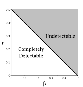
Figure 2: Detection boundaries for the heteroscedastic normal mixture model. Left: (Sparse case for $\sigma_{0}\in\{0.4,0.8,1,1.2,\sqrt{2},2,4\}$) Above the boundary is the completely detectable area and underneath is the undetectable area for both tests (LLR and HC). The limits $\xi_{1}$ and $\xi_{2}$ are Gaussian on the linear part (solid) and non-Gaussian on the quadratic part (dashed). In both cases the HC test has no asymptotic power. On the vertical dotted line $P(\xi_{2}\in\mathbb{R})\in(0,1)$. Right: (dense case for $\sigma_{0}^{2}=1$) Above the boundary is the undetectable area and underneath is the completely detectable area for both tests. On the boundary the limits $\xi_{1}$ and $\xi_{2}$ are Gaussian and the HC test has no power.

The results concerning ARE can also be applied for the heteroscedastic models. Fix the variance parameter $\sigma_{0}>0$. Let $\boldsymbol{\theta_{1}}=(\beta_{1},r_{1})$ and $\boldsymbol{\theta_{2}}=(\beta_{2},r_{2})$ represent two models from the linear part (I) of the detection boundary leading to Gaussian limits of $T_{n}$. Suppose that the models are different, i.e. $\beta_{1}\neq\beta_{2}$. By applying Theorem 2.6 and simple calculations, which are omitted to the reader, $\mathrm{ARE}=0$ can be shown. That means that the LLR test $\varphi_{n}(\boldsymbol{\theta_{2}})$ can not distinguish between the null and the alternative asymptotically when $\boldsymbol{\theta_{1}}$ is the true, underlying model. As already mentioned $\gamma(\boldsymbol{\theta_{j}},\boldsymbol{\theta_{j}})=\sigma^{2}_{j}$ does not hold if $\beta_{j}=1-\sigma_{0}^{2}/4$. In this case make use of the truncation Lemma A.3.
Cai et al. [5] already considered the dense case $\beta<1/2$. In this case $\sigma_{0}^{2}\neq 1$ always leads to the completely detectable case independently of how the signal strength $\vartheta_{n}$ is chosen. Thus, only the heterogeneous case $\sigma_{0}^{2}=1$ is of real interest. In this case the parametrisation $\vartheta_{n}=n^{r}$ is used for $r>0$. The corresponding detection boundary is given by $\rho(\beta)=1/2-\beta$ and is plotted in Figure 2. The HC test achieves the same region of complete detection, see [5]. Our results concerning the tests’ power behaviour on the detection boundary can also be applied. In short, on the detection boundary (2.12) holds for some $\sigma>0$ and the HC test has no asymptotic power there. This is even possible to a general class of one-parametric exponential families including the dense heterogeneous normal mixtures. To not overload this paper, we omit further details concerning the dense case and refer the reader to the thesis of Ditzhaus [10].

Appendix A Gaussian limits

Gaussian limits $\xi_{1}$ and $\xi_{2}$, compare to (2.12), are of special interest, for example regarding Theorem 2.6. Recall that the degenerate case is included as $\sigma=0$. In the following we give several equivalent conditions for Gaussian limits.

Theorem A.1 (Gaussian limits).

The conditions (a)-(i) are equivalent:

1. $\xi_{1}$ and $\xi_{2}$ are Gaussian or $\xi_{1}=\xi_{2}\equiv 0$ with probability one.

2. $\xi_{1}\sim N(-\frac{\sigma^{2}}{2},\sigma^{2})$ for some $\sigma^{2}\in[0,\infty)$.

3. $\xi_{2}\sim N(\frac{\sigma^{2}}{2},\sigma^{2})$ for some $\sigma^{2}\in[0,\infty)$.

4. $\xi_{2}$ is real-valued and $\xi_{1}\sim N(a,\sigma^{2})$ for some $a\in\mathbb{R}$, $\sigma^{2}\in[0,\infty)$.

5. $\xi_{2}\sim N(a,\sigma^{2})$ for some $a\in\mathbb{R}$, $\sigma^{2}\in[0,\infty)$.

6. $Z_{n}$ given by (A.1) converges in distribution under $P_{(n)}$ to some normal distributed $Z\sim N(0,\sigma^{2})$ for some $\sigma^{2}\in[0,\infty)$:

   (A.1) $$Z_{n}=\sum_{i=1}^{k_{n}}\varepsilon_{n,i}\Bigl{(}\frac{\mathrm{d}\mu_{n,i}}{\,\mathrm{d}P_{n,i}}-1\Bigr{)}\overset{\mathrm{d}}{\longrightarrow}Z.$$

7. $\xi_{2}$ is real-valued and $\max_{1\leq i\leq k_{n}}\frac{\mathrm{d}Q_{n,i}}{\,\mathrm{d}P_{n,i}}\to 1\textrm{ in }P_{(n)}\textrm{-probability}$.

8. $\xi_{2}$ is real-valued and $\max_{1\leq i\leq k_{n}}\varepsilon_{n,i}\frac{\mathrm{d}\mu_{n,i}}{\,\mathrm{d}P_{n,i}}\to 0\textrm{ in }P_{(n)}\textrm{-probability}$.

9. For some $\tau\in(0,\infty)$ and all $x>0$ we have $I_{n,1,x}\to 0$ and $I_{n,2,\tau}\to\sigma^{2}\in[0,\infty)$.

If one of the conditions (b)–(f) or (i) is fulfilled for some $\sigma^{2}\in[0,\infty)$ then the others do so for the same $\sigma^{2}$.

Remark A.2.

Theorem A.1(i) holds for some $\tau>0$ if and only if it does for all.

To apply Theorem 2.6 $\gamma(\boldsymbol{\theta},\boldsymbol{\theta})=\sigma^{2}$ is needed, where $\sigma^{2}$ comes from the previous section and $\boldsymbol{\theta}$ denotes the underlying model, compare to the notation in Section 2.3. As already mentioned there are examples, for which this equation fails although $\xi_{1}$ and $\xi_{2}$ are normal distributed. But by truncation we can always ensure the equality without changing the asymptotic results.

Lemma A.3 (Truncation).

Let the assumptions of Theorem A.1 and one of its equivalent conditions (a)-(i) be fulfilled. In order to use a truncation argument define

$$\widetilde{\varepsilon}_{n,i}=\varepsilon_{n,i}\mu_{n,i}\Bigl{(}\varepsilon_{n,i}\frac{\mathrm{d}\mu_{n,i}}{\,\mathrm{d}P_{n,i}}\leq\tau\Bigr{)}\text{ for some }\tau>0$$

and let $\widetilde{\mu}_{n,i}$ be given as follows: if $\widetilde{\varepsilon}_{n,i}=0$ then $\frac{\mathrm{d}\widetilde{\mu}_{n,i}}{\,\mathrm{d}P_{n,i}}=1$, and otherwise

$$\frac{\mathrm{d}\widetilde{\mu}_{n,i}}{\,\mathrm{d}P_{n,i}}=\frac{\mathrm{d}\mu_{n,i}}{\,\mathrm{d}P_{n,i}}\mathbf{1}\Bigl{\{}\varepsilon_{n,i}\frac{\mathrm{d}\mu_{n,i}}{\,\mathrm{d}P_{n,i}}\leq\tau\Bigr{\}}\Bigl{[}\mu_{n,i}\Bigl{(}\varepsilon_{n,i}\frac{\mathrm{d}\mu_{n,i}}{\,\mathrm{d}P_{n,i}}\leq\tau\Bigr{)}\Bigr{]}^{-1}.$$

All our asymptotic results in this paper remain the same if we replace $\mu_{n,i}$ and $\varepsilon_{n,i}$ by $\widetilde{\mu}_{n,i}$ and $\widetilde{\varepsilon}_{n,i}$.

Appendix B Proofs

In the following we give all the proofs. These are not given in the order of their appearance since we apply, for example, Theorem 2.4 to verify Theorem 2.2. Before giving the proofs we introduce some useful properties of binary experiments and generalise limit theorems of Gnedenko and Kolmogorov [15] to infinitely divisible distributions.

B.1 Binary experiments and distances for probability measures

Binary experiments classify different types of signal detectability. This gives us a first rough insight in the different detection regions for our signal detection problem. This standard approach is recalled for a sequence of binary experiments $\{\widetilde{P}_{(n)},{\widetilde{Q}}_{(n)}\}$, $n\in\mathbb{N}\cup\{0\}$, where the underlying measurable spaces $(\Omega_{n},{\mathcal{A}}_{n})$ may change with $n$. Recall the equivalence of the weak convergences in (B.1) and (B.2) on $[-\infty,\infty]$:

(B.1) $${\mathcal{L}}\Bigl{(}\log\frac{\mathrm{d}\widetilde{Q}_{(n)}}{\,\mathrm{d}\widetilde{P}_{(n)}}\Bigr{|}\widetilde{P}_{(n)}\Bigr{)}\; \overset{\mathrm{w}}{\longrightarrow}\;{\mathcal{L}}\Bigl{(}\log\frac{\mathrm{d}\widetilde{Q}_{(0)}}{\,\mathrm{d}\widetilde{P}_{(0)}}\Bigr{|}\widetilde{P}_{(0)}\Bigr{)}=\nu_{1}\textrm{ (say)},$$

(B.2) $${\mathcal{L}}\Bigl{(}\log\frac{\mathrm{d}\widetilde{Q}_{(n)}}{\,\mathrm{d}\widetilde{P}_{(n)}}\Bigr{|}\widetilde{Q}_{(n)}\Bigr{)}\; \overset{\mathrm{w}}{\longrightarrow}\;{\mathcal{L}}\Bigl{(}\log\frac{\mathrm{d}\widetilde{Q}_{(0)}}{\,\mathrm{d}\widetilde{P}_{(0)}}\Bigr{|}\widetilde{Q}_{(0)}\Bigr{)}=\nu_{2}\textrm{ (say)}.$$

Following Le Cam we say that $\{\widetilde{P}_{(n)},\widetilde{Q}_{(n)}\}$ converges weakly to $\{\nu_{1},\nu_{2}\}$ ($\{\widetilde{P}_{(0)},\widetilde{Q}_{(0)}\}$, respectively) if and only if (B.1) or (B.2) is fulfilled. Note that every sequence of binary experiments has at least one accumulation point in the sense of weak convergence, see Lemma 60.6 of Strasser [34]. In general $\nu_{1}$ is a measure on $\mathbb{R}\cup\{-\infty\}$ and $\nu_{2}$ is one on $\mathbb{R}\cup\{\infty\}$ connected by

(B.3) $$\frac{\,\mathrm{d}\nu_{2|\mathbb{R}}}{\,\mathrm{d}\nu_{1|\mathbb{R}}}(x)=e^{x}\textrm{ and }\nu_{2}(\{-\infty\})=1-\int e^{x}\,\mathrm{d}\nu_{1}(x).$$

Using the terminology of weak convergence of binary experiments we can express the different types of (asymptotic) detectability as follows:

• completely detectable: $\{P_{(n)},Q_{(n)}\}$ converges weakly to the so called full informative experiment $\{\nu_{1},\nu_{2}\}=\{\epsilon_{-\infty},\epsilon_{\infty}\}$.

• undetectable: $\{P_{(n)},Q_{(n)}\}$ converges weakly to the so called uninformative experiment $\{\nu_{1},\nu_{2}\}=\{\epsilon_{0},\epsilon_{0}\}$.

• detectable: None (weak) accumulation point of $\{P_{(n)},Q_{(n)}\}$ is the uninformative experiment $\{\nu_{1},\nu_{2}\}=\{\epsilon_{0},\epsilon_{0}\}$.

The variational distance of probability measures $\widetilde{P}$ and $\widetilde{Q}$ on a common measure space $(\widetilde{\Omega},\widetilde{\mathcal{A}})$ is given by

(B.4) $$||\widetilde{P}-\widetilde{Q}||=\sup\{E_{\widetilde{P}}(\varphi)-E_{\widetilde{Q}}(\varphi):\textrm{ measurable }\varphi:\widetilde{\Omega}\to[0,1]\},$$

see Lemma 2.3 of Strasser [34]. It is easy to show that weak convergence of $\{\widetilde{P}_{(n)},\widetilde{Q}_{(n)}\}$ to $\{\widetilde{P}_{(0)},\widetilde{Q}_{(0)}\}$ implies convergence of the variational distance $||\widetilde{P}_{(n)}-\widetilde{Q}_{(n)}||\to||\widetilde{P}_{(0)}-\widetilde{Q}_{(0)}||$. Our three cases can be reformulated to:

• completely detectable: $||P_{(n)}-Q_{(n)}||$ tends to $1$.

• undetectable: $||P_{(n)}-Q_{(n)}||$ tends to $0$.

• detectable: We have $\liminf_{n\to\infty}||P_{(n)}-Q_{(n)}||>0$.

For product measures the Hellinger distance $d$ is useful:

(B.5) $$d^{2}(\widetilde{P},\widetilde{Q})=\frac{1}{2}\int\Bigl{(}\Bigl{(}\frac{\,\mathrm{d}\widetilde{P}}{\,\mathrm{d}\nu}\Bigr{)}^{\frac{1}{2}}-\Bigl{(}{\frac{\,\mathrm{d}\widetilde{Q}}{\,\mathrm{d}\nu}}\Bigr{)}^{\frac{1}{2}}\Bigr{)}^{2}\,\mathrm{d}\nu=1-\int\Bigl{(}\frac{\,\mathrm{d}\widetilde{P}}{\,\mathrm{d}\nu}\frac{\,\mathrm{d}\widetilde{Q}}{\,\mathrm{d}\nu}\Bigr{)}^{\frac{1}{2}}\,\mathrm{d}\nu,$$

where $\widetilde{P},\widetilde{Q}\ll\nu$. Since $d^{2}({\widetilde{P}},{\widetilde{Q}})\leq||{\widetilde{P}}-{\widetilde{Q}}||\leq\sqrt{2}\,d({\widetilde{P}},{\widetilde{Q}})$, see Lemma 2.15 of [34], we obtain from (1.1) and (1.3) that

(B.6) $$\max_{i=1,\ldots,k_{n}}d^{2}(P_{n,i},Q_{n,i})\leq\max_{1\leq i\leq k_{n}}||P_{n,i}-Q_{n,i}||\leq\max_{1\leq i\leq k_{n}}\varepsilon_{n,i}\to 0.$$

Consequently, $d^{2}(P_{(n)},Q_{(n)})=1-\prod_{i=1}^{k_{n}}(1-d^{2}(P_{n,i},Q_{n,i}))$ tends to $b\in[0,1]$ if and only if $-\log(1-b)$ is the limit of

(B.7) $$D_{n}=\sum_{i=1}^{k_{n}}d^{2}(P_{n,i},Q_{n,i}).$$

To sum up, we get the following characterisation of the trivial detection regions.

Lemma B.1.

1. We are in the undetectable case if and only if $D_{n}\to 0$.

2. We are in completely detectable case if and only if $D_{n}\to\infty$.

Note that from the connection between the variational distance and the Hellinger distance we obtain

(B.8) $$\frac{1}{2}\sum_{i=1}^{k_{n}}\varepsilon_{n,i}^{2}\>||P_{n,i}-\mu_{n,i}||^{2}\leq D_{n}\leq\sum_{i=1}^{k_{n}}\varepsilon_{n,i}\>||P_{n,i}-\mu_{n,i}||.$$

B.2 Limit theorems

For the readers’ convenience let us recall well known convergence results of Gnedenko and Kolmogorov [15] which we use rapidly. Let $(Y_{n,i})_{1\leq i\leq k_{n}}$ be a triangular array of row-wise independent, infinitesimal, real-valued random variables on some probability space $(\Omega,{\mathcal{A}},P)$. In our case we have

(B.9) $$\sum_{i=1}^{k_{n}}P(Y_{n,i}\leq x)=0$$

for all fixed $x<0$ if $n\geq N_{x}$ is sufficiently large. Combining this with (9) of Chap. 3.18, Theorem 4.25.4 and the subsequent remark of [15] yields:

Theorem B.2.

We have distributional convergence

$$\sum_{i=1}^{k_{n}}Y_{k_{n},i}\overset{\mathrm{d}}{\longrightarrow}Y$$

to some real-valued $Y$ on $\left(\Omega,\mathcal{A},P\right)$ if and only if the following conditions (i)-(iii) hold.

1. There is a Lévy measure $\eta$ on $\mathbb{R}\setminus\{0\}$ such that $\eta(-\infty,0)=0$ and

   $$\sum_{i=1}^{k_{n}}P\left(Y_{k_{n},i}>x\right)\to\eta(x,\infty)\in\mathbb{R}\textrm{ as }n\to\infty$$

   for all $x\in C_{+}(\eta)$, i.e. for all continuity points of $t\mapsto\eta(t,\infty)$, $t>0$.

2. There exists some constant $\sigma^{2}\in[0,\infty)$ such that

   $$\sigma^{2}=\lim_{\varepsilon\searrow 0}\;\underset{n\to\infty}{\begin{subarray}{c}\limsup\\ \liminf\end{subarray}}\;\sum_{i=1}^{k_{n}}\int_{\left\{\left|Y_{k_{n},i}\right|<\varepsilon\right\}}Y_{k_{n},i}^{2}\,\mathrm{d}P-\sum_{i=1}^{k_{n}}\left(\int_{\left\{\left|Y_{k_{n},i}\right|<\varepsilon\right\}}Y_{k_{n},i}\,\mathrm{d}{P}\right)^{2}.$$

3. There is some constant $\gamma\in\mathbb{R}$ and $\tau_{0}\in C_{+}(\eta)$ such that

   $$\lim_{n\to\infty}\sum_{i=1}^{k_{n}}\int Y_{k_{n},i}\mathbf{1}{\left\{\left|Y_{k_{n},i}\right|<\tau_{0}\right\}}\,\mathrm{d}P$$

   $$=\gamma+\int_{(-\tau_{0},\tau_{0})\setminus\{0\}}\frac{x^{3}}{1+x^{2}}\,\,\mathrm{d}\eta(x)-\int_{\mathbb{R}\setminus[-\tau_{0},\tau_{0}]}\frac{x}{1+x^{2}}\,\,\mathrm{d}\eta(x).$$

Under (i)-(iii) $Y$ is infinitely divisible with Lévy-Khintchine triplet $(\gamma,\sigma^{2},\eta)$.

As stated in Theorem 2.4, we have to deal also with positive weights in $\infty$ for the limits since $\nu_{2}=\rho+(1-a)\epsilon_{-\infty}$, where $a<1$ may occur.

Theorem B.3.

Suppose that the conditions (ii) and (iii) of Theorem B.2 hold for some $\tau_{0}\in C_{+}(M_{0})$. Assume that the following (a) and (b) hold.

1. There is a dense subset $\mathcal{D}$ of $(0,\infty)$ and a measure $M_{0}$ on $(0,\infty]$ with

   $$\sum_{i=1}^{k_{n}}P\left(Y_{k_{n},i}>x\right)\;\to\;\,M_{0}(x,\infty]\in\mathbb{R}\text{ for all }x\in{\mathcal{D}}.$$

2. There exists some $\tau_{1}>0$ such that

   $$\limsup_{n\to\infty}\sum_{i=1}^{k_{n}}\int_{\left\{\left|Y_{k_{n},i}\right|<\tau_{1}\right\}}Y_{k_{n},i}^{2}\,\mathrm{d}P<\infty.$$

Then,

$${\mathcal{L}}\Bigl{(}\sum_{i=1}^{k_{n}}Y_{n,i}\Bigr{)}\overset{\mathrm{w}}{\longrightarrow}e^{-M_{0}(\{\infty\})}\nu+(1-e^{-M_{0}(\{\infty\})})\epsilon_{\infty},$$

where $\nu$ is a infinitely divisible measure on $\mathbb{R}$ with Lévy-Khintchine triplet $(\gamma,\sigma^{2},\eta)$ and Lévy measure $\eta=M_{0|(0,\infty)}$.

Proof.

Put $\eta=M_{0|(0,\infty)}$. Let the sequence $(M_{n})_{n\in\mathbb{N}}$ consists of measures on $(0,\infty]$ given by $M_{n}(x,\infty]=\sum_{i=1}^{k_{n}}P(Y_{n,i}>x)$, $x>0$. Clearly, $M_{n|(0,\infty)}\overset{\mathrm{w}}{\longrightarrow}\eta$ and $\limsup_{n\to\infty}\int_{(0,\tau_{1})}t^{2}\,\mathrm{d}M_{n}(t)<\infty$. Thus, we obtain $\int\min(t^{2},1)\,\mathrm{d}\eta(t)<\infty$, which proves that $\eta$ is a Lévy measure. Define $Z_{n,u}=\sum_{i=1}^{k_{n}}Y_{n,i}\mathbf{1}\{Y_{n,i}\leq u\}$ for all $u\in{\mathcal{D}}$, $u>\tau_{0}$. By Theorem B.2 $Z_{n,u}$ converges in distribution to $X_{u}$, where $X_{u}$ is infinitely divisible with Lévy-Khintchine triplet $(\gamma_{u},\sigma^{2},\eta_{u})$, Lévy measure $\eta_{u}=\eta_{(0,u]}$ and shift term

$$\gamma_{u}=\gamma-\int_{(u,\infty)}\frac{x}{1+x^{2}}\,\mathrm{d}\eta(x).$$

Since $\eta$ is Lévy measure it is easy to verify $\gamma_{u}\to\gamma$ as ${\mathcal{D}}\ni u\to\infty$. By this and Theorem 3.19.2 of [15] $X_{u}$ converges in distribution to $X$ as ${\mathcal{D}}\ni u\to\infty$, where $X\sim\nu$. Now, let $(u_{n})_{n\in\mathbb{N}}$ be a sequence in ${\mathcal{D}}$ which tends to $\infty$ slowly enough such that $\sum_{i=1}^{k_{n}}P\left(Y_{k_{n},i}>u_{n}\right)\;\to\;\,M_{0}(\{\infty\}).$ Standard arguments, see Theorem 3.2 of Billingsley [4], imply that $Z_{n,u_{n}}$ converges in distribution to $X$ since for all $\delta>0$

$$\limsup_{n\to\infty}P\Bigl{(}\Bigl{|}Z_{n,u}-Z_{n,u_{n}}\Bigr{|}\geq\delta\Bigl{)}\leq M_{0}(u,\infty)\to 0\text{ as }{\mathcal{D}}\ni u\to\infty.$$

The basic idea to determine the limit distribution of $\sum_{i=1}^{k_{n}}Y_{n,i}$ is to condition on $C_{n}=\{\max_{1\leq i\leq k_{n}}Y_{n,i}\leq u_{n}\}$. Note that for all $t\in\mathbb{R}$

$$P\Bigl{(}\sum_{i=1}^{k_{n}}Y_{n,i}\leq t\Bigr{)}=P(Z_{n,u_{n}}\leq t|C_{n})P(C_{n})+P\Bigl{(}\sum_{i=1}^{k_{n}}Y_{n,i}\leq t,\max_{1\leq i\leq k_{n}}Y_{n,i}>u_{n}\Bigr{)},$$

where the latter summand tends to $0$. Moreover, observe that

$$1-P(C_{n})=\prod_{i=1}^{k_{n}}\Bigl{(}1-P(Y_{n,i}>u_{n})\Bigr{)}\to e^{-M_{0}(\{\infty\})}.$$

It is remains to show that $Z_{n,u_{n}}$ tends to $X$ conditioned on $C_{n}$. Conditioned on $C_{n}$ we have $Z_{n,u_{n}}=\sum_{i=1}^{k_{n}}Y_{n,i}\mathbf{1}\{Y_{n,i}\leq u_{n}\}$ and $(Y_{n,i}\mathbf{1}\{Y_{n,i}\leq u_{n}\})_{i\leq k_{n}}$ is a rowwise independent and infinitesimal triangular array. Hence, we can apply Theorem B.2 to $Z_{n,u_{n}}$ conditioned on $C_{n}$. Finally, by basic calculations Theorem B.2(i)-(iii) are fulfilled for the same $\eta$, $\sigma^{2}$ and $\gamma$ given by the Lévy-Khintchine triplet of the limit X of $Z_{n,u_{n}}$, e.g. we have for all $x\in{\mathcal{D}}$

$$\sum_{i=1}^{k_{n}}P\Bigl{(}Y_{n,i}\mathbf{1}\{Y_{n,i}\leq u_{n}\}>x|C_{n}\Bigr{)}=\sum_{i=1}^{k_{n}}\frac{P(Y_{n,i}>x)-P(Y_{n,i}>u_{n})}{P(Y_{n,i}\leq u_{n})}\to\eta(x,\infty)$$

since $\min_{1\leq i\leq k_{n}}P(Y_{n,i}\leq u_{n})\geq 1-\max_{1\leq i\leq k_{n}}P(Y_{n,i}\geq 1)\to 1$.

B.3 Proofs of Section 2 and Appendix A

B.3.1 Proof of Theorem 2.1

The statement of Theorem 2.1 follows immediately from the following lemma.

Lemma B.4.

Let $I_{n,1,x}$ and $I_{n,2,x}$, $x>0$, be defined as in in (2.4) and (2.5), respectively. Let $D_{n}$ be defined as in (B.7). Then we have for all $\tau>0$:

1. There exists a constant $C_{\tau}>0$ such that

   (B.10) $$D_{n}\leq\Bigl{(}\frac{1}{2}+\max_{1\leq i\leq k_{n}}\varepsilon_{n,i}\Bigr{)}I_{n,1,\tau}+I_{n,2,\tau}$$

   (B.11) $$D_{n}\geq C_{\tau}\max\Bigl{\{}I_{n,1,\tau},I_{n,2,\tau}-\frac{2}{\tau}I_{n,1,\tau}\max_{1\leq i\leq k_{n}}\varepsilon_{n,i}\Bigr{\}}.$$

Remark B.5.

The idea and the proof of the upper bound of $D_{n}$ in (B.10) is based on the argumentation of Cai et al. [5] on pp. 21f.

Lemma B.4.

To shorten the notation, we define

(B.12) $$A_{n,i,x}=\Bigl{\{}\varepsilon_{n,i}\frac{\mathrm{d}\mu_{n,i}}{\,\mathrm{d}P_{n,i}}>x\Bigr{\}}\textrm{ for all }x>0.$$

We can deduce from (B.5) that

(B.13) $$D_{n}\,\leq\;\sum_{i=1}^{k_{n}}\mbox{I\negthinspace E}_{P_{n,i}}\left(1-\>\sqrt{1-\varepsilon_{n,i}+\varepsilon_{n,i}\frac{\mathrm{d}\mu_{n,i}}{\,\mathrm{d}P_{n,i}}\mathbf{1}(A_{n,i,\tau}^{c})}\>\right).$$

Note that $1-\sqrt{1+t}\leq-t/2+t^{2}$ for all $t\geq-1$. Applying this (pointwisely) to the integrand in (B.13) with $t=\varepsilon_{n,i}(\frac{\mathrm{d}\mu_{n,i}}{\,\mathrm{d}P_{n,i}}\mathbf{1}(A_{n,i,\tau}^{c})-1)$ yields (B.10).
We split the proof of (B.11) into two steps. First, define for all $x>0$

(B.14) $$\widetilde{I}_{n,2,x} =\sum_{i=1}^{k_{n}}\int_{A_{n,i,x}^{c}}\varepsilon_{n,i}^{2}\Bigl{(}\frac{\mathrm{d}\mu_{n,i}}{\,\mathrm{d}P_{n,i}}-1\Bigr{)}^{2}\,\mathrm{d}P_{n,i}.$$

For $\varepsilon_{n}^{\text{max}}=\max_{1\leq i\leq k_{n}}\varepsilon_{n,i}$ we can deduce from $\varepsilon_{n}^{\text{max}}\geq(\varepsilon_{n}^{\text{max}})^{2}$ and

(B.15) $$\sum_{i=1}^{k_{n}}P_{n,i}(Y_{n,i}>x)\leq\sum_{i=1}^{k_{n}}P_{n,i}(A_{n,i,e^{x}-1})\leq\frac{1}{e^{x}-1}I_{n,1,e^{x}-1}$$

(B.16) $$\text{that }-\frac{2\varepsilon_{n}^{\text{max}}}{x}I_{n,1,x}\leq\widetilde{I}_{n,2,x}-I_{n,2,x}\leq 2\varepsilon_{n}^{\text{max}}I_{n,1,x}$$

for all $x>0$. Since $\mathrm{d}Q_{n,i}/\mathrm{d}P_{n,i}$ is bounded from above by $1+\tau$ on $A_{n,i,\tau}^{c}$ we obtain

$$2D_{n}\;\geq\;\sum_{i=1}^{k_{n}}\int\Bigl{(}1-\frac{\mathrm{d}Q_{n,i}}{\,\mathrm{d}P_{n,i}}\Bigr{)}^{2}\Bigl{(}1+\Bigl{(}\frac{\mathrm{d}Q_{n,i}}{\,\mathrm{d}P_{n,i}}\Bigr{)}^{1/2}\Bigr{)}^{-2}\mathbf{1}(A_{n,i,\tau}^{c})\,\mathrm{d}P_{n,i}\geq\frac{\widetilde{I}_{n,2,\tau}}{(1+\sqrt{{1+\tau}})^{2}}.$$

Combining this and (B.16) gives us the first bound in (B.14) for appropriate $C_{\tau}$. Second, set $C=1/(\sqrt{\tau/2+1}+1)<1/2$. Note that on $A_{n,i,\tau}$

$$\Bigl{(}\frac{\mathrm{d}Q_{n,i}}{\,\mathrm{d}P_{n,i}}\Bigr{)}^{1/2}-1=\Bigl{(}\frac{\mathrm{d}Q_{n,i}}{\,\mathrm{d}P_{n,i}}-1\Bigr{)}\Bigl{(}\Bigl{(}\frac{\mathrm{d}Q_{n,i}}{\,\mathrm{d}P_{n,i}}\Bigr{)}^{1/2}+1\Bigr{)}^{-1}\leq C\left(\frac{\mathrm{d}Q_{n,i}}{\,\mathrm{d}P_{n,i}}-1\right).$$

Consequently,

$$2\>D_{n} \geq\sum_{i=1}^{k_{n}}E_{P_{n,i}}\Bigl{(}\Bigl{(}\frac{\mathrm{d}Q_{n,i}}{\,\mathrm{d}P_{n,i}}-1-2\Bigr{(}\Bigl{(}\frac{\mathrm{d}Q_{n,i}}{\,\mathrm{d}P_{n,i}}\Bigr{)}^{1/2}-1\Bigr{)}\Bigr{)}\mathbf{1}(A_{n,i,\tau})\Bigr{)}$$

$$\geq(1-2C)\left(1-\frac{\max_{1\leq i\leq k_{n}}\varepsilon_{n,i}}{\tau}\right)\sum_{i=1}^{k_{n}}\varepsilon_{n,i}\mu_{n,i}\left(A_{n,i,\tau}\right).$$

Finally, (a) is shown and combining it with Lemma B.1 yields (a) and (b).

B.3.2 Proof of Theorem 2.2(b)

The statements follows from Remark (8.6) and Lemma (8.7) of Janssen et al. [22] as we explain in the following. Let $C^{2}_{lok}(\mathbb{R})$ be set of all bounded functions $f:\mathbb{R}\to\mathbb{R}$ that are twice differentiable with continuous derivatives in some neighbourhood of $0$. Denote by $f^{(k)}(0)$ the kth derivative of $f$ at $0$. The Lévy-Khintchine triplet of a infinitely divisible measure $\nu$ is equal to $(\gamma,\sigma^{2},\eta)$ if and only if the generating functional $A:C^{2}_{lok}(\mathbb{R})\to\mathbb{R}$ admits the Lévy-Khintchine representation

$$A(f)=f^{(1)}(0)\gamma+\sigma^{2}f^{(2)}(0)+\int_{\mathbb{R}\setminus\{0\}}\Bigl{(}f(x)-f(0)-\frac{f^{(1)}(0)x}{1+x^{2}}\Bigr{)}\,\mathrm{d}\eta(x)$$

for all $f\in C^{2}_{lok}(\mathbb{R})$. For the actual definition of $A$ and more details about it we refer the reader to Janssen et al. [22], in particular to (8.1)-(8.4).

Lemma B.6.

Let $\{\widetilde{\nu}_{1},\widetilde{\nu}_{2}\}$ be some binary experiment in its standard form, compare to (B.1) and (B.2), such that $\widetilde{\nu_{1}}(\mathbb{R})=\widetilde{\nu}_{2}(\mathbb{R})=1$ and $\widetilde{\nu}_{1}$ is infinitely divisible with Lévy-Khintchine triplet $(\gamma,\sigma^{2},\eta)$. Then $\widetilde{\nu}_{2}$ is also infinitely divisible with Lévy-Khintchine triplet $(\gamma_{2},\sigma^{2}_{2},\eta_{2})$, where $\sigma_{1}^{2}=\sigma^{2}_{2}$, $\eta_{2}\ll\eta_{1}$ with Radon-Nikodym derivative $x\mapsto\mathrm{d}\eta_{2}/\mathrm{d}\eta_{1}(x)=e^{x}$ and

(B.17) $$\gamma_{1}+\frac{\sigma^{2}_{1}}{2}-\int\Bigl{(}1-e^{x}+\frac{x}{x^{2}+1}\Bigr{)}\,\mathrm{d}\eta_{1}(x)=0,$$

(B.18) $$\gamma_{2}=\gamma_{1}+\sigma_{1}^{2}+\int(e^{x}-1)\frac{x}{1+x^{2}}\,\mathrm{d}\eta_{1}(x).$$

Remark B.7.

Since $\int x^{2}\mathbf{1}(|x|\leq 1)\,\mathrm{d}\eta_{1}(x),\int e^{x}\mathbf{1}(|x|\geq 1)\,\mathrm{d}\eta_{1}(x)<\infty$, see Lemma (8.7)(a) of [22], the integrals in (B.17) and (B.18) are finite.

Lemma B.6.

Let $A$ be the generating functional of $\widetilde{\nu}_{1}$. Combining $\int\exp\,\mathrm{d}\widetilde{\nu}_{1}=\widetilde{\nu}_{2}(\mathbb{R})=1$ and Lemma (8.7)(b) and (c) from [22] we deduce that $A(\exp)=0$ and $C^{2}_{lok}(\mathbb{R})\ni f\mapsto A(\exp f)$ is the generating functional of $\widetilde{\nu}_{2}$ and, in particular, $\widetilde{\nu}_{2}$ is infinitely divisible. Using the Lévy-Khintchine representation of $A$ immediately yields that $A(\exp)$ is equal to the left side of (B.17), which proves (B.17). From $f(0)A(\exp)=0$ we get for all $f\in C^{2}_{lok}(\mathbb{R})$

$$A(f\exp) =f^{(1)}(0)\Bigl{(}\gamma_{1}+\sigma^{2}_{1}+\int(e^{x}-1)\frac{x}{1+x^{2}}\,\mathrm{d}\eta_{1}(x)\Bigr{)}$$

$$\phantom{=}+f^{(2)}(0)\frac{\sigma^{2}_{1}}{2}+\int\Bigl{(}f(x)-f(0)-\frac{f^{(1)}(0)x}{1+x^{2}}\Bigr{)}e^{x}\,\mathrm{d}\eta_{1}(x).$$

Consequently, the statements about $(\gamma_{2},\sigma_{2}^{2},\eta_{2})$ follow.

Now, we prove Theorem 2.2(b). Since $\frac{\mathrm{d}Q_{n,i}}{\,\mathrm{d}P_{n,i}}\geq 1-\max_{1\leq i\leq k_{n}}\varepsilon_{n,i}\to 1$ (B.9) is fulfilled and by Theorem B.2 $\eta_{1}$ is concentrated on $(0,\infty)$. Now, consider $\{\widetilde{\nu}_{1},\widetilde{\nu}_{2}\}=\{\nu_{1}*\epsilon_{-\log(a)},(a^{-1}\nu_{2|\mathbb{R}})*\epsilon_{-\log(a)}\}$. This binary experiment is in its standard from since

$$\frac{\,\mathrm{d}\widetilde{\nu}_{2}}{\,\mathrm{d}\widetilde{\nu}_{1}}(x)=a^{-1}\frac{\,\mathrm{d}\nu_{2}}{\,\mathrm{d}\nu_{1}}(x+\log(a))=\exp(x),\,x\in\mathbb{R}.$$

Clearly, $\widetilde{\nu}_{1}$ is infinitely divisible with Lévy characteristic $(\gamma_{1}-\log(a),\sigma_{1}^{2},\eta_{1})$ and $\widetilde{\nu}_{1}(\mathbb{R})=\widetilde{\nu}_{2}(\mathbb{R})=1$. Applying Lemma B.6 proves that $\widetilde{\nu}_{2}$ is infinitely divisible and so is $\rho=a^{-1}\nu_{2|\mathbb{R}}$. Moreover, is easy to check that we obtain all statements about the Lévy-Khintchine triplets.

B.3.3 Proof of Theorem 2.4

We carried out two different proofs for Theorem 2.4. The first one relies on infinitely divisible statistical experiments and accompanying Poisson experiments, and arguments from Chap. 4, 5, 9, 10 of Janssen et al. [22] are used. The second one is based on traditional limit theorems for real-valued random variables. Since, probably, the second one is easier to follow for the readers who are not experts in the field of statistical experiments we decided to present only the second proof.
At the end of the proof we will verify the following lemma.

Lemma B.8.

Suppose that (a) and (b) hold. Then the sums in Theorem B.2 (ii) and (iii) and in Theorem B.3(a) and (b) for $Y_{n,i}$ defined by

(B.19) $$Y_{n,i}=\log\frac{\mathrm{d}Q_{n,i}}{\,\mathrm{d}P_{n,i}}$$

are upper bounded for every $x>0$ and all sufficiently small $\tau_{0},\tau_{1}\in{\mathcal{D}}$, respectively, under $P_{(n)}$ as well as under $Q_{(n)}$. In particular, Theorem B.2(ii) is fulfilled for $\sigma^{2}$ under $P_{(n)}$.

Let us first assume that (a) and (b) are fulfilled. Define $Y_{n,i}$ as in (B.19). Regarding Lemma B.8 and using typical sub-subsequence arguments we can assume without loss of generality that Theorem B.2(i) and (ii) as well as Theorem B.3(a) and (b) hold for a measure $M_{1}$ (resp. $M_{2}$), $\sigma_{1}\geq 0$ ($\sigma_{2}\geq 0$, resp.) and $\gamma_{1}\in\mathbb{R}$ ($\gamma_{2}\in\mathbb{R}$, resp.) under $P_{(n)}$ ($Q_{(n)}$, resp.). In particular, by Lemma B.8 $\sigma_{1}^{2}=\sigma^{2}$. Note that $\eta_{j}=M_{j|(0,\infty)}$ is a Lévy measure. From (B.15) we obtain $M_{1}(\{\infty\})=0$ and so $\xi_{1}$, the limit of $T_{n}$ under $P_{(n)}$, is real-valued. Moreover, since $\max_{1\leq i\leq k_{n}}\varepsilon_{n,i}\to 0$ and $\varepsilon_{n,i}\mu_{n,i}(A_{n,i,e^{x}-1+\varepsilon_{n,i}})=Q_{n,i}(Y_{n,i}>x)-(1-\varepsilon_{n,i})P_{n,i}(Y_{n,i}>x)$ we can deduce that $M_{|(0,\infty)}=\eta_{2}-\eta_{1}$ and $M_{2}(\{\infty\})=M(\{\infty\})$. Finally, the proof for the first assertion is completed by Theorem 2.2(b).
Now, let $\xi_{1}$ be not equal to $-\infty$ with probability one. By Theorem 2.1(a) we have $\sup_{n\in\mathbb{N}}I_{n,1,\tau}+I_{n,2,\tau}<\infty$ for all $\tau>0$. Hence, for each subsequence there is a subsequence such that (a) for some measure $M$ and (b) for some $\sigma^{2}$ are fulfilled. From Theorem 2.2(b) and the first assertion proved above we obtain: $\xi_{1}$ is real-valued, and $M$ and $\sigma^{2}$ are uniquely determined by the distribution of $\xi_{1}$ and so do not depend on the special choice of the subsequence, which proves the second assertion (and Theorem 2.2(a)).

Lemma B.8.

First, observe that by (B.15) the sum in Theorem B.3(a) is upper bounded under $P_{(n)}$ as well as under $Q_{(n)}$ for all $\tau>0$. By (1.3)

(B.20) $$B_{n,i,\tau}=\left\{\left|Y_{n,i}\right|\leq\tau\right\}=A_{n,i,t_{n,i}(\tau)}^{c}$$

if $n\geq N_{\tau}$ is sufficiently large, where $t_{n,i}(\tau)=e^{\tau}-1+\varepsilon_{n,i}\in[e^{\tau}-1,e^{\tau}]$. Define $\widetilde{I}_{n,2,x}$ as in (B.14). By Taylor’s formula there exists some random variable $R_{n,i,\tau}$ with $R_{n,i,\tau}=0$ on $B^{c}_{n,i,\tau}$ such that we have on $B_{n,i,\tau}$

(B.21) $$Y_{n,i}=\varepsilon_{n,i}\Bigl{(}\frac{\mathrm{d}\mu_{n,i}}{\,\mathrm{d}P_{n,i}}-1\Bigr{)}-\varepsilon_{n,i}^{2}\Bigl{(}\frac{\mathrm{d}\mu_{n,i}}{\,\mathrm{d}P_{n,i}}-1\Bigr{)}^{2}\Bigl{(}\frac{1}{2}+R_{n,i,\tau}\Bigr{)}$$

and $\max_{1\leq i\leq k_{n}}|R_{n,i,\tau}|\leq C_{\tau}$ for some constant $C_{\tau}\in(0,\infty)$ with $C_{\tau}\to 0$ as $\tau\searrow 0$. Combining this and (B.15) yields

$$\Bigl{|}\sum_{i=1}^{k_{n}}\int_{B_{n,i,\tau}}Y_{n,i}\,\mathrm{d}P_{n,i}\Bigr{|}\leq\Bigl{(}1+\frac{1}{e^{\tau}-1}\Bigr{)}I_{n,1,e^{\tau}-1}+\Bigl{(}\frac{1}{2}+C_{\tau}\Bigr{)}\widetilde{I}_{n,2,e^{\tau}},$$

where by (B.16) the upper bound is bounded itself for all sufficiently small $\tau>0$. Since $Q_{n,i}=(1-\varepsilon_{n,i})P_{n,i}+\varepsilon_{n,i}\mu_{n,i}$ and $\frac{\mathrm{d}\mu_{n,i}}{\,\mathrm{d}P_{n,i}}\leq e^{\tau}$ on $B_{n,i,\tau}$ we obtain similarly the following upper bound of $|\sum_{i=1}^{k_{n}}\int_{B_{n,i,\tau}}Y_{n,i}\,\mathrm{d}Q_{n,i}|$:

$$\Bigl{|}\sum_{i=1}^{k_{n}}\int_{B_{n,i,\tau}}Y_{n,i}\,\mathrm{d}P_{n,i}\Bigr{|}+I_{n,1,e^{\tau}-1}+\Bigl{(}1+\Bigl{(}\frac{1}{2}+C_{\tau}\Bigr{)}e^{\tau}\Bigr{)}\widetilde{I}_{n,2,e^{\tau}},$$

which itself is bounded for all small $\tau>0$, see also (B.16). In the last step we discuss the sum in Theorem B.2(ii). On $B_{n,i,\tau}$ we obtain the following inequalities from (B.21) for all sufficiently small $\tau>0$ such that $C_{\tau}\leq\frac{1}{2}$:

$$\varepsilon_{n,i}\Bigl{|}\frac{\mathrm{d}\mu_{n,i}}{\,\mathrm{d}P_{n,i}}-1\Bigr{|}\left(2-e^{\tau}-2\varepsilon_{n,i}\right)\leq|Y_{n,i}|\leq\varepsilon_{n,i}\Bigl{|}\frac{\mathrm{d}\mu_{n,i}}{\,\mathrm{d}P_{n,i}}-1\Bigr{|}\left(e^{\tau}+2\varepsilon_{n,i}\right).$$

From this, (B.16) and $\frac{\mathrm{d}Q_{n,i}}{\,\mathrm{d}P_{n,i}}\leq e^{\tau}+\max_{1\leq i\leq k_{n}}\varepsilon_{n,i}$ on $B_{n,i,\tau}$ we conclude

$$\lim_{\tau\searrow 0}\;\underset{n\to\infty}{\begin{subarray}{c}\limsup\\ \liminf\end{subarray}}\sum_{i=1}^{k_{n}}\int_{B_{n,i,\tau}}Y_{n,i}^{2}\,\mathrm{d}Q_{n,i}\leq\lim_{\tau\searrow 0}\;\underset{n\to\infty}{\begin{subarray}{c}\limsup\\ \liminf\end{subarray}}\sum_{i=1}^{k_{n}}\int_{B_{n,i,\tau}}Y_{n,i}^{2}\,\mathrm{d}P_{n,i}=\sigma^{2}.$$

Since $(a+b)^{2}\leq 4a^{2}+4b^{2}$ we have for all sufficiently small $\tau>0$ that

$$\frac{1}{4}\sum_{i=1}^{k_{n}}\Bigl{(}\int_{B_{n,i,\tau}}Y_{n,i}\,\mathrm{d}P_{n,i}\Bigr{)}^{2}$$

$$\leq\sum_{i=1}^{k_{n}}\Bigl{(}\varepsilon_{n,i}\int_{B_{n,i,\tau}^{c}}1-\frac{\mathrm{d}\mu_{n,i}}{\,\mathrm{d}P_{n,i}}\,\mathrm{d}P_{n,i}\Bigr{)}^{2}+\Bigl{(}\int_{B_{n,i,\tau}}\varepsilon_{n,i}^{2}\Bigl{(}\frac{\mathrm{d}\mu_{n,i}}{\mathrm{d}P_{n,i}}-1\Bigr{)}^{2}\,\mathrm{d}P_{n,i}\Bigr{)}^{2}$$

$$\leq\Bigl{(}\max_{1\leq i\leq k_{n}}\varepsilon_{n,i}\Bigr{)}(1+\tau)I_{n,1,e^{\tau}-1}+\widetilde{I}_{n,2,e^{\tau}}(e^{\tau}-1+\max_{1\leq i\leq k_{n}}\varepsilon_{n,i})^{2}.$$

Hence, by (B.16) $\lim_{\tau\searrow 0}\limsup_{n\to\infty}(\int_{B_{n,i,\tau}}Y_{n,i}\,\mathrm{d}P_{n,i})^{2}=0$ and, consequently, Theorem B.2(ii) is fulfilled for $\sigma^{2}$ under $P_{(n)}$.

B.3.4 Proof of Theorem 2.2(a)

We verified Theorem 2.2(a) while proving the second assertion of Theorem 2.4. ´

B.3.5 Proof of Theorem A.1

The equivalence of (a)-(e) follows from (B.3) and is standard for binary experiments, see Strasser [34]. The equivalence of (g) and (h) follows from (1.1) and (1.3). Define $A_{n,i,x}$ as in (B.12).

Equivalence of (b) and (i): By Theorem 2.4 $I_{n,1,x}\to 0$ for all $x>0$ holds also under (b). Hence, we can suppose that this convergence is fulfilled subsequently. Fix $\tau>0$. Then

$$0\leq E_{P_{n,i}}\left(\varepsilon_{n,i}^{2}\Bigl{(}\frac{\mathrm{d}\mu_{n,i}}{\,\mathrm{d}P_{n,i}}\Bigr{)}^{2}\mathbf{1}\Bigl{\{}\frac{\mathrm{d}\mu_{n,i}}{\,\mathrm{d}P_{n,i}}\in(x,\tau]\Bigr{\}}\right)\leq\tau\>\varepsilon_{n,i}\mu_{n,i}(A_{n,i,x})$$

holds for all $x\in(0,\tau]$ and so $I_{n,2,x}-I_{n,2,\tau}\to 0$ does. Consequently, (i) holds if and only if Theorem 2.4(a) and (b) do so for the same $\sigma^{2}\in[0,\infty)$ and $M\equiv 0$. Hence, the equivalence of (b) and (i) follows from Theorem 2.4.

Equivalence of (f) and (i): Define $Y_{n,i}$ as in (B.19) and set $\widetilde{Y}_{n,i}=f(Y_{n,i})$ for $f(x)=\exp(x)-1$, $x\in\mathbb{R}$. Note that $f(0)=0$ and $f^{\prime}(0)=f^{\prime\prime}(0)=1$. From this, a Taylor expansion, compare to (B.21), and Theorem B.2 we obtain that $\sum_{i=1}^{k_{n}}Y_{n,i}$ converges in distribution to $X$ with Lévy-Khintchine triplet $(0,\sigma^{2},0)$ if and only if $\sum_{i=1}^{k_{n}}\widetilde{Y}_{n,i}$ does so to $\widetilde{X}$ with Lévy-Khintchine triplet $(-\sigma^{2}/2,\sigma^{2},0)$.

Equivalence of (d) and (h): Throughout this proof step we can assume that $\xi_{2}$ is real-valued and so is $\xi_{1}$, see Theorem 2.2(a). By the first Lemma of Le Cam $P_{(n)}$ and $Q_{(n)}$ are mutually contiguous, see also Remark 2.3. Hence, (h) is true if and only if for all $x>0$

$$0\leftarrow Q_{(n)}\Bigl{(}\max_{1\leq i\leq k_{n}}\varepsilon_{n,i}\frac{\mathrm{d}\mu_{n,i}}{\,\mathrm{d}P_{n,i}}>x\Bigr{)}=1-\prod_{i=1}^{k_{n}}\Bigl{(}1-Q_{n,i}(A_{n,i,x})\Bigr{)}.$$

Combining this and (B.15) yields that (h) is fulfilled if and only if $I_{n,1,x}\to 0$ for all $x>0$. Finally, note that $\xi_{1}$ is normal distributed if and only if it has trivial Lévy measure $\eta_{1}\equiv 0$, which by Theorem 2.4 is true if and only if $I_{n,1,x}\to 0$ for all $x>0$.

B.3.6 Proof of Lemma A.3

Let $\widetilde{Q}_{n,i}$ and $\widetilde{Q}_{(n)}$ be defined as $Q_{n,i}$ and $Q_{(n)}$ replacing $\mu_{n,i}$ and $\varepsilon_{n,i}$ by $\widetilde{\mu}_{n,i}$ and $\widetilde{\varepsilon}_{n,i}$. For the statement in Lemma A.3 it is sufficient to show that $\{Q_{(n)},\widetilde{Q}_{n,i}\}$ tend weakly to the uninformative experiment $\{\epsilon_{0},\epsilon_{0}\}$. The main task for this purpose is to verify $\sum_{i=1}^{k_{n}}||Q_{n,i}(\boldsymbol{\theta})-Q_{n,i}(\boldsymbol{\widetilde{\theta}})||\to 0$, which is left to the reader.

B.3.7 Proof of Theorem 2.6

Denote by $Z_{n}(\boldsymbol{\theta_{1}})$ and $Z_{n}(\boldsymbol{\theta_{2}})$ the statistic introduced in (A.1) for the model $\boldsymbol{\theta_{1}}$ and $\boldsymbol{\theta_{2}}$, respectively. Since these statistics are linear, the multivariate central limit theorem implies distributional convergence $(Z_{n}(\boldsymbol{\theta_{1}}),Z_{n}(\boldsymbol{\theta_{2}}))\overset{\mathrm{d}}{\longrightarrow}\widetilde{Z}\sim N((0,0),(\gamma(\boldsymbol{\theta_{i}},\boldsymbol{\theta_{j}}))_{1\leq i,j\leq 2})$ under $P_{(n)}$. In the next step we verify for $j=1,2$

(B.22) $$T_{n}(\boldsymbol{\theta_{j}})=Z_{n}(\boldsymbol{\theta_{j}})-\frac{\gamma(\boldsymbol{\theta_{j}},\boldsymbol{\theta_{j}})}{2}+R_{n,j},$$

where $R_{n,j}$ converges in $P_{(n)}$-probability to $0$. Let $j\in\{1,2\}$ be fixed. Define $Y_{n,i}^{(j)}=\varepsilon_{n,i}^{(j)}(\mathrm{d}\mu_{n,i}^{(j)}/\,\mathrm{d}P_{n,i}^{(j)}-1)$. Note that by Taylor’s Theorem $\log(1+x)=x-\frac{x^{2}}{2}+(2/3)x^{3}(1+y_{x})^{-3}$ for $|y_{x}|\leq x$. Since $\max_{1\leq i\leq k_{n}}Y_{n,i}^{(j)}\to 0$ in $P_{(n)}$-probability, see Theorem A.1, it remains to shown that $\sum_{i=1}^{k_{n}}(Y_{n,i}^{(j)})^{2}\to\gamma(\boldsymbol{\theta_{j}},\boldsymbol{\theta_{j}})$ in $P_{(n)}$-probability. It is well know that this follows immediately if the Lindeberg condition is fulfilled for the triangular array $(Y_{n,i}^{(j)})_{i\leq k_{n}}$ under $P_{(n)}$. Observe that combining Theorem A.1(f) and the assumption $\gamma(\boldsymbol{\theta_{j}},\boldsymbol{\theta_{j}})=\sigma_{j}^{2}$ yields the desired Lindeberg condition and, finally, (B.22).
From (B.22) and the asymptotic normality of the vector $(Z_{n}(\boldsymbol{\theta_{1}}),Z_{n}(\boldsymbol{\theta_{2}}))$ we obtain $(T_{n}(\boldsymbol{\theta_{1}}),T_{n}(\boldsymbol{\theta_{2}}))\overset{\mathrm{d}}{\longrightarrow}\widehat{Z}\sim N((-\gamma(\boldsymbol{\theta_{j}},\boldsymbol{\theta_{j}})/2)_{j=1,2},(\gamma(\boldsymbol{\theta_{i}},\boldsymbol{\theta_{j}}))_{1\leq i,j\leq 2})$. Consequently, by the third lemma of Le Cam we get under $Q_{(n)}(\boldsymbol{\theta_{1}})$

$$(T_{n}(\boldsymbol{\theta_{1}}),T_{n}(\boldsymbol{\theta_{2}}))\overset{\mathrm{d}}{\longrightarrow}\widehat{Z}\sim N\Bigl{(}\Bigl{(}\frac{-\gamma(\boldsymbol{\theta_{j}},\boldsymbol{\theta_{j}})}{2}+\gamma(\boldsymbol{\theta_{1}},\boldsymbol{\theta_{j}})\Bigr{)}_{j=1,2},(\gamma(\boldsymbol{\theta_{i}},\boldsymbol{\theta_{j}}))_{1\leq i,j\leq 2}\Bigr{)}.$$

Finally, the desired statement can be concluded.

B.3.8 Proof of Corollary 2.8

Define

$$\varepsilon^{*}_{n,i}=\frac{\varepsilon_{n,i}(1-\kappa_{n,i})}{1-\varepsilon_{n,i}\kappa_{n,i}}.$$

Now, let $Q_{n,i}^{*}$, $Q_{(n)}^{*}$ and $T_{n}^{*}$ defined as $\widetilde{Q}_{n,i}$, $\widetilde{Q}_{(n)}$ and $\widetilde{T}_{n}$ replacing $\widetilde{\varepsilon}_{n,i}$ by $\varepsilon_{n,i}^{*}$. Since $\widetilde{\varepsilon}_{n,i}=\varepsilon_{n,i}^{*}(1+a_{n,i})$ with $\max_{1\leq i\leq k_{n}}|a_{n,i}|\to 0$ it can easily be seen by Theorems 2.2 and 2.4 that (2.3) also holds for $T_{n}^{*}$ with the same limits $\widetilde{\xi}_{1}$ and $\widetilde{\xi}_{2}$. Note that

$$\frac{\mathrm{d}Q_{n,i}}{\,\mathrm{d}P_{n,i}}=(1-\varepsilon_{n,i}\kappa_{n,i})\frac{\mathrm{d}Q_{n,i}^{*}}{\,\mathrm{d}P_{n,i}}+\infty\>\mathbf{1}_{N_{n,i}}\mathbf{1}\{\kappa_{n,i}>0\}.$$

Since $\bigotimes_{i=1}^{k_{n}}N_{n,i}$ is a $P_{(n)}$-null set we obtain that $P_{(n)}$-almost surely

$$\log\Bigl{(}\frac{\mathrm{d}Q_{(n)}}{\,\mathrm{d}P_{(n)}}\Bigr{)} =\log\Bigl{(}\frac{\mathrm{d}Q_{(n)}^{*}}{\,\mathrm{d}P_{(n)}}\Bigr{)}+\sum_{i=1}^{k_{n}}\log(1-\kappa_{n,i}\varepsilon_{n,i}).$$

Combining this and $\sum_{i=1}^{k_{n}}\log(1-\kappa_{n,i}\varepsilon_{n,i})\to-c$ yields that $T_{n}\overset{\mathrm{d}}{\longrightarrow}\widetilde{\xi}_{1}-c=\xi_{1}$ under $P_{(n)}$. By Section B.1 we obtain that $T_{n}$ converges in distribution to some $\xi_{2}$ under $Q_{(n)}$ and by (B.3) we get the desired representation $\nu_{2}=e^{-c}\widetilde{\nu}_{2}*\epsilon_{-c}+(1-e^{-c})\epsilon_{\infty}$ of $\xi_{2}$’s distribution .

B.4 Proofs of Section 3

To shorten the notation we define

$$Z_{n}(t)=\sqrt{n}\;\frac{\mathbb{F}_{n}(t)-t}{\sqrt{t(1-t)}},\,t\in(0,1).$$

Then,

$$HC_{n}=\sup_{t\in(0,1)}|Z_{n}(t)|.$$

B.4.1 Proof of Theorem 3.1

First, note that

$$a_{n}HC_{n}-b_{n}=\sqrt{2}\,\log\log\left(k_{n}\right)\,\left(\frac{HC_{n}}{\sqrt{\log\log(k_{n})}}-\sqrt{2}+o(1)\right).$$

That is why it sufficient to show that for some $\gamma>0$

(B.23) $$Q_{(n)}\Bigl{(}\frac{|Z_{n}(v_{n})|}{\sqrt{\log\log k_{n}}}\leq\sqrt{2}+\gamma\Bigr{)}\to 0$$

(B.24) or $$Q_{(n)}\Bigl{(}\frac{|Z_{n}(1-v_{n})|}{\sqrt{\log\log k_{n}}}\leq\sqrt{2}+\gamma\Bigr{)}\to 0.$$

To verify this we apply Chebyshev’s inequality. Note that for every real-valued random variable $Z$ on some probability space $(\Omega,{\mathcal{A}},P)$ with finite expectation we have

(B.25) $$P\left(\left|Z\right|\leq\frac{|E(Z)|}{2}\right)=P\left(\left|Z-E(Z)\right|\geq\frac{\left|E(Z)\right|}{2}\right)\leq 4\frac{\text{Var}_{P}(Z)}{E_{P}(Z)^{2}}.$$

Consequently, we need to determine first the expectation and variance for $Z_{n}(v)$ for $v\in\{v_{n},1-v_{n}\}$:

$$E_{Q_{(n)}}(Z_{n}(v)) =\sqrt{k_{n}}\;\frac{k_{n}^{-1}\sum_{i=1}^{k_{n}}Q_{n,i}(0,v]-v}{\sqrt{v(1-v)}}=\frac{\sum_{i=1}^{k_{n}}\varepsilon_{n,i}\left(\mu_{n,i}\left(0,v\right]-v\right)}{\sqrt{k_{n}\,v(1-v)}}\;,$$

$$\text{Var}_{Q_{(n)}}(Z_{n}(v)) =\;\frac{1}{k_{n}}\;\frac{\sum_{i=1}^{k_{n}}Q_{n,i}(0,v]\left(1-Q_{n,i}(0,v]\right)}{v(1-v)}$$

$$\leq\min\Bigl{\{}\frac{\sum_{i=1}^{k_{n}}Q_{n,i}(0,v]}{k_{n}\,v(1-v)}\;,\;\frac{\sum_{i=1}^{k_{n}}(1-Q_{n,i}(0,v])}{k_{n}\,v(1-v)}\Bigr{\}}$$

$$=\min\Bigl{\{}\frac{1}{1-v}+\frac{E_{Q_{(n)}}\left[Z_{n}\left(v\right)\right]}{\sqrt{k_{n}\,v(1-v)}}\;,\;\frac{1}{v}-\frac{E_{Q_{(n)}}\left[Z_{n}\left(v\right)\right]}{\sqrt{k_{n}\,v(1-v)}}\Bigr{\}}.$$

By assumption we have

(B.26) $$\frac{|\sum_{i=1}^{k_{n}}\varepsilon_{n,i}(\mu_{n,i}(0,v_{n}]-v_{n})|}{\sqrt{k_{n}v_{n}\log\log(k_{n})}}\to\infty$$

(B.27) or $$\frac{|\sum_{i=1}^{k_{n}}\varepsilon_{n,i}(\mu_{n,i}(1-v_{n},1)-v_{n})|}{\sqrt{k_{n}v_{n}\log\log k_{n}}}\to\infty.$$

Suppose that (B.26) holds. Then

$$\left|\frac{E_{Q_{(n)}}(Z_{n}(v_{n}))}{\sqrt{\log\log(k_{n})}}\right|\to\infty\textrm{ and }\frac{\text{Var}_{Q_{(n)}}(Z_{n}(v_{n}))}{E_{Q_{(n)}}(Z_{n}(v_{n}))^{2}}\to 0.$$

Combining this and (B.25) yields that (B.23) is fulfilled for all $\gamma>0$. Analogously, if (B.27) is true then (B.24) holds for all $\gamma>0$.

B.4.2 Proof of Theorem 3.2

Let $G_{n}$ be the distribution function of $Q_{n,1}$, i.e. $G_{n}(v)=Q_{n,1}([0,v])$, $v\in(0,1)$. Let $U_{1},U_{2},\ldots$ be a sequence of independent, uniformly on $(0,1)$ distributed random variables on the same probability space $(\Omega,{\mathcal{A}},P)$. Note $(U_{1},\ldots,U_{k_{n}})\sim P_{(n)}$ and $(G_{n}^{-1}(U_{1}),\ldots,G_{n}^{-1}(U_{k_{n}}))\sim Q_{(n)}$, where $G_{n}^{-1}$ denotes the left continuous quantile function of $Q_{n,1}$. Moreover, denote the interval $(r_{n},s_{n})\cup(t_{n},u_{n})$ by $J_{n,1}$ and $[1-u_{n},1-t_{n}]\cup[1-s_{n},1-r_{n}]$ by $J_{n,2}$. By (3.3) it is easy to see that we can replace $r_{n}$ by any $r_{n}^{\prime}\geq r_{n}$ such that $\log(r_{n}^{\prime})=(-1+o(1))\log(n)$. In particular, we can assume without loss of generality that $k_{n}r_{n}\geq 1$ and, analogously, $u_{n}<1/2$. From Corollaries 2 and 3 as well as (1) and (2) of Theorem of Jaeschke [21], which also hold for the statistics $W_{n},\widehat{V}_{n},\widehat{W}_{n}$ introduced at the beginning of subsection 2 therein, we can deduce that

(B.28) $$a_{n}\sup_{v\in(0,1)\setminus(J_{n,1}\cup J_{n,2})}\Bigl{\{}\;\Bigl{|}\frac{\sum_{i=1}^{k_{n}}(\mathbf{1}\{U_{i}\leq v\}-v)}{\sqrt{k_{n}v(1-v)}}\Bigr{|}\Bigr{\}}-b_{n}\overset{\mathrm{P}}{\longrightarrow}-\infty$$

(B.29) and $$a_{n}\sup_{v\in(0,1)}\Bigl{\{}\;\Bigl{|}\frac{\sum_{i=1}^{k_{n}}(\mathbf{1}\{U_{i}\leq v\}-v)}{\sqrt{k_{n}v(1-v)}}\Bigr{|}\Bigr{\}}-b_{n}\overset{\mathrm{d}}{\longrightarrow}Y,$$

where the distribution function of $Y$ equals $\Lambda^{2}$, see (3.1). By (B.28), the mutually contiguity of $P_{(n)}$ and $Q_{(n)}$ and the equivalence ”$G_{n}(v)\geq u\Leftrightarrow v\geq G_{n}^{-1}(u)$” it is sufficient for (3.5) to verify

(B.30) $$a_{n}\sup_{v\in J_{n,1}\cup J_{n,2}}\Bigl{\{}\;\frac{\sum_{i=1}^{k_{n}}(\mathbf{1}\{U_{i}\leq G_{n}(v)\}-v)}{\sqrt{k_{n}v(1-v)}}\Bigr{\}}-b_{n}\overset{\mathrm{d}}{\longrightarrow}Y.$$

For this purpose we define

$$\Delta_{n,1}(v)=\frac{\sum_{i=1}^{k_{n}}\left(\mathbf{1}\{U_{i}\leq{G}_{n}(v)\}-{G}_{n}(v)\right)}{\sqrt{n\,{G}_{n}(v)(1-{G}_{n}(v))}},$$

$$\Delta_{n,2}(v)=\sqrt{\frac{{G}_{n}(v)}{v}},\;\Delta_{n,3}(v)=\sqrt{\frac{1-{G}_{n}(v)}{(1-v)}},\;\Delta_{n,4}(v)=\sqrt{k_{n}}\,\frac{{G}_{n}(v)-v}{\sqrt{\,v(1-v)}}.$$

Clearly,

$$\frac{\sum_{i=1}^{k_{n}}\left(\mathbf{1}\{U_{i}\leq{G}_{n}(v)\}-v\right)}{\sqrt{k_{n}\,v(1-v)}}\;=\;\Delta_{n,1}(v)\Delta_{n,2}(v)\Delta_{n,3}(v)+\Delta_{n,4}(v).$$

Hence, the proof of (B.30) falls naturally into the following steps:

(B.31) $$\sup_{v\in J_{n,1}\cup J_{n,2}}\left|\Delta_{n,j}(v)-1\right|\to 0\textrm{ for }j\in\{2,3\},$$

(B.32) $$a_{n}\sup_{v\in J_{n,1}\cup J_{n,2}}\left|\Delta_{n,4}(v)\right|\to 0,$$

(B.33) $$\ a_{n}\sup_{v\in J_{n,1}\cup J_{n,2}}\{|\Delta_{n,1}(v)|\}-b_{n}\overset{\mathrm{d}}{\longrightarrow}Y.$$

First, observe that $(1-\varepsilon_{n})v\leq G_{n}(v)\leq v+\varepsilon_{n}(1-v)$ for all $v\in(0,1)$. Hence, we have for all $v_{1}\in(0,1/2]$ and $v_{2}\in[1/2,1)$ that

$$\frac{1-G_{n}(v_{1})}{1-v_{1}},\,\frac{G_{n}(v_{2})}{v_{2}}\in(1-\varepsilon_{n},1+\varepsilon_{n}).$$

Moreover, we have for all $v_{1}\in J_{n,1}$ and all $v_{2}\in J_{n,2}$ that

(B.34) $$\left|\frac{{G}_{n}\left(v_{1}\right)}{v_{1}}-1\right| =\frac{\varepsilon_{n}|\mu_{n}(0,v_{1}]-v_{1}|}{v_{1}}\leq\frac{H_{n}(v_{1})}{\sqrt{k_{n}r_{n}}}\leq a_{n}H_{n}(v_{1}),$$

(B.35) $$\left|\frac{1-{G}_{n}\left(v_{2}\right)}{1-v_{2}}-1\right| =\frac{\varepsilon_{n}|\mu_{n}(v_{2},1)-(1-v_{2})|}{1-v_{2}}\,\leq a_{n}H_{n}(1-v_{2}).$$

Consequently, (B.31) follows. Similarly to the above, we obtain

$$|\Delta_{n,4}(v_{1})|\leq\frac{H_{n}(v_{1})}{\sqrt{1-u_{n}}}\leq\frac{1}{\sqrt{2}}H_{n}(v_{1})\textrm{ and }|\Delta_{n,4}(v_{2})|\leq\frac{1}{\sqrt{2}}H_{n}(1-v_{2}).$$

for all $v_{1}\in J_{n,1}$ and $v_{2}\in J_{n,2}$. From this we obtain (B.32). Clearly,

$$\sup_{v\in J_{n,1}\cup J_{n,2}}|\Delta_{n,1}(v)|=\sup_{v\in\widetilde{J}_{n,1}\cup\widetilde{J}_{n,2}}\Bigl{|}\frac{\sum_{i=1}^{k_{n}}(\mathbf{1}\{U_{i}\leq v\}-v)}{\sqrt{k_{n}v(1-v)}}\Bigr{|},$$

where $\widetilde{J}_{n,1}=[\widetilde{r}_{n},\widetilde{s}_{n}]\cup[\widetilde{t}_{n},\widetilde{u}_{n}]$ by $\widehat{J}_{n,2}=(1-\widehat{u}_{n},1-\widehat{t}_{n})\cup(1-\widehat{s}_{n},1-\widehat{r}_{n})$ with $\widetilde{r}_{n}=G_{n}(r_{n})$, $\widetilde{s}_{n}=G_{n}(s_{n})$, $\widetilde{t}_{n}=G_{n}(t_{n})$, $\widetilde{u}_{n}=G_{n}(u_{n})$, $\widehat{r}_{n}=1-G_{n}(1-r_{n})$, $\widehat{s}_{n}=1-G_{n}(1-s_{n})$, $\widehat{t}_{n}=1-G_{n}(1-t_{n})$ and $\widehat{u}_{n}=1-G_{n}(1-u_{n})$. From (B.34), (B.35) and (3.3) we deduce that ($\widetilde{r}_{n}$,$\widetilde{s}_{n}$,$\widetilde{t}_{n}$,$\widetilde{u}_{n}$) and ($\widehat{r}_{n}$,$\widehat{s}_{n}$,$\widehat{t}_{n}$,$\widehat{u}_{n}$) fulfil (3.4). Finally, (B.33) follows from (B.28) and (B.29) (with the new parameters).

B.5 Proofs of Section 4.1

Before we prove the theorems stated in Section 4.1 we want to point out the following: We can always assume that there is no perturbation, i.e. $r_{n,i}=0$ for all $i,n$, see Lemma B.9. Note that we will assume this in all upcoming proofs concerning Section 4.1 without recalling it every time.

Lemma B.9 (Perturbation).

Let us consider the situation in Section 4.1. Let $\mu_{n,i}^{*}$, $Q_{n,i}^{*}$ and $Q_{(n)}^{*}$ be defined as $\mu_{n,i}$, $Q_{n,i}$ and $Q_{(n)}$ setting $r_{n,i}=0$ for all $i,n$. Then (4.2) is a sufficient that $\{Q_{(n)},Q_{(n)}^{*}\}$ converges weakly to the uninformative experiment $\{\epsilon_{0},\epsilon_{0}\}$. In other words, if (4.2) is fulfilled then the perturbation by $(r_{n,i})_{i\leq k_{n}}$ does not affect the asymptotic results.

Proof.

It is sufficient to show that $\sum_{i=1}^{k_{n}}d^{2}(Q_{n,i},Q_{n,i}(\boldsymbol{\widetilde{\theta}}))\to 0$ under (4.2). This convergence follows immediately from the first representation of the Hellinger distance in (B.5) and the third binomial formula:

$$2d^{2}(Q_{n,i},Q_{n,i}(\boldsymbol{\widetilde{\theta}}))$$

$$=\int_{0}^{1}\frac{(\varepsilon_{n,i}r_{n,i})^{2}}{(\sqrt{(1-\varepsilon_{n,i})+\varepsilon_{n,i}h_{n,i}}+\sqrt{(1-\varepsilon_{n,i})+\varepsilon_{n,i}h_{n,i}+\varepsilon_{n,i}r_{n,i}})^{2}}\,\mathrm{d}\lambda\!\!\!\;\!\lambda$$

$$\leq\frac{\varepsilon_{n,i}^{2}}{1-\varepsilon_{n,i}}\int_{0}^{1}r_{n,i}^{2}\,\mathrm{d}\lambda\!\!\!\;\!\lambda.$$

B.5.1 Proof of Theorem 4.1

First, observe that

(B.36) $$I_{n,1,x}=\sum_{i=1}^{k_{n}}\varepsilon_{n,i}\int_{0}^{1}h_{n,i}\,\mathbf{1}\Bigr{\{}\frac{\varepsilon_{n,i}}{\kappa_{n,i}}h_{n,i}>x\Bigl{\}}\,\mathrm{d}\lambda\!\!\!\;\!\lambda,$$

(B.37) $$I_{n,2,x}=\sum_{i=1}^{k_{n}}\Bigl{(}\frac{\varepsilon_{n,i}^{2}}{\kappa_{n,i}}\int_{0}^{1}h_{n,i}^{2}\,\mathbf{1}\Bigr{\{}\frac{\varepsilon_{n,i}}{\kappa_{n,i}}h_{n,i}\leq x\Bigl{\}}\,\mathrm{d}\lambda\!\!\!\;\!\lambda\Bigr{)}-\sum_{i=1}^{k_{n}}\varepsilon_{n,i}^{2}.$$

Moreover, note that

(B.38) $$I_{n,1,x} \leq\frac{1}{x}\sum_{i=1}^{k_{n}}\frac{\varepsilon_{n,i}^{2}}{\kappa_{n,i}}\int h_{n,i}^{2}\,\mathbf{1}\Bigr{\{}\frac{\varepsilon_{n,i}}{\kappa_{n,i}}h_{n,i}>x\Bigl{\}}\,\mathrm{d}\lambda\!\!\!\;\!\lambda,$$

$$I_{n,1,x}+I_{n,2,x} \leq\max\{1,x^{-1}\}\Bigl{(}\max_{1\leq i\leq k_{n}}\int_{0}^{1}h_{n,i}^{2}\,\mathrm{d}\lambda\!\!\!\;\!\lambda\Bigr{)}\sum_{i=1}^{k_{n}}\frac{\varepsilon_{n,i}^{2}}{\kappa_{n,i}}$$

By these and Theorem 2.1 $K=0$ corresponds to the undetectable case and no accumulation point of $\{P_{(n)},Q_{(n)}\}$ is full informative if $K\in(0,\infty)$. By Lemma B.1(b) and (B.8) the latter is also valid if $\limsup_{n\to\infty}\sum_{i=1}^{k_{n}}\varepsilon_{n,i}<\infty$. Consequently, (a) and the first statement in (c) are verified. Now, let us suppose that $K\in(0,\infty)$ and (4.5) holds. Clearly, $\sum_{i=1}^{k_{n}}\varepsilon_{n,i}^{2}\to 0$. By (B.37) and (B.38) $I_{n,1,x}\to 0$ and $I_{n,2,x}\to K\int_{0}^{1}h^{2}\,\mathrm{d}\lambda\!\!\!\;\!\lambda=\sigma^{2}$ for all $x>0$. Hence, applying Theorem 2.4 completes the proof of (c).
Now, let the assumptions of (b) hold. Without loss of generality we can assume that $\sum_{i=1}^{k_{n}}\varepsilon_{n,i}^{2}\to C_{1}<\infty$ and $\varepsilon_{n,r_{n}}/\kappa_{n,r_{n}}\to C\in[0,\infty]$ since otherwise we use standard sub-subsequence arguments and make use of (B.8). If $C\geq 1$ then for all sufficiently large $n\in\mathbb{N}$

$$I_{n,1,x} \geq\sum_{i=r_{n}}^{k_{n}}\varepsilon_{n,i}\int_{0}^{1}h_{n,i}\,\mathbf{1}\Bigr{\{}\frac{\varepsilon_{n,r_{n}}}{\kappa_{n,r_{n}}}h_{n,i}>x\Bigl{\}}\,\mathrm{d}\lambda\!\!\!\;\!\lambda$$

$$\geq\Bigl{(}\sum_{i=r_{n}}^{k_{n}}\varepsilon_{n,i}\Bigr{)}\min_{1\leq i\leq k_{n}}\int_{0}^{1}h_{n,i}\,\mathbf{1}\Bigr{\{}\frac{1}{2}h_{n,i}>x\Bigl{\}}\,\mathrm{d}\lambda\!\!\!\;\!\lambda$$

and so by (4.3) $I_{n,1,x}\to\infty$ for all sufficiently small $x>0$. If $C<1$ then

$$I_{n,2,x} \geq\Bigl{(}\sum_{i=1}^{r_{n}}\frac{\varepsilon_{n,i}^{2}}{\kappa_{n,i}}\Bigr{)}\min_{1\leq i\leq k_{n}}\int_{0}^{1}h_{n,i}^{2}\,\mathbf{1}\Bigr{\{}2h_{n,i}\leq x\Bigl{\}}\,\mathrm{d}\lambda\!\!\!\;\!\lambda-C_{1}$$

and so by (4.3) $I_{n,2,x}\to\infty$ for all sufficiently large $x>0$. Hence, applying Theorem 2.1 verifies (b). Finally, note that $K<\infty$ implies $\sum_{i=1}^{k_{n}}\varepsilon_{n,i}^{2}\to 0$. Keeping this in mind the proof of (d) is trivial (and omitted to the reader).

B.5.2 Proof of Theorem 4.3

By (B.37)

$$-\frac{1}{k_{n}}\leq I_{n,2,x}\leq\frac{x}{k_{n}}\sum_{i=1}^{k_{n}}\int_{0}^{1}h_{n,i}\mathbf{1}\{k_{n}^{r-1}h_{n,i}\leq x\}\,\mathrm{d}\lambda\!\!\!\;\!\lambda\leq x$$

$$\textrm{and so }\lim_{x\searrow 0}\underset{n\to\infty}{\begin{subarray}{c}\limsup\\ \liminf\end{subarray}}\,\,I_{n,2,x}=0.$$

Combining (B.36) and (4.6) yields for all $x\in{\mathcal{D}}$ that $I_{n,1,e^{x}-1}$ equals

$$\frac{1}{k_{n}}\sum_{i=1}^{k_{n}}\int_{0}^{1}h_{n,i}\,\mathbf{1}\Bigr{\{}k_{n}^{r-1}h_{n,i}>e^{x}-1\Bigl{\}}\,\mathrm{d}\lambda\!\!\!\;\!\lambda\to\mathbf{1}\{r>1\}+M(x,\infty)\mathbf{1}\{r=1\}.$$

Consequently, applying Theorem 2.4 and Theorem 2.1 completes the proof.

B.5.3 Proof of Theorem 4.5

It is easy to verify that by (B.36) and (B.37)

$$I_{n,1,x}=\min\Bigl{\{}n^{1-\beta},n^{\frac{1}{\alpha}(\alpha-\beta+r(1-\alpha))}\Bigl{(}\frac{x}{1-\alpha}\Bigr{)}^{1-\frac{1}{\alpha}}\Bigr{\}},\;\,I_{n,2,x}\leq n^{1-2\beta+r}.$$

Note that $1-2\beta+r<0$ if $r<\rho^{*}(\beta,\alpha)$, or if $r=\rho^{*}(\beta,\alpha)$ and $\alpha>1/2$. Moreover, in the case of $\alpha=1/2$, $r=\rho^{*}(\beta,\alpha)=2\beta-1$ we have

$$I_{n,2,x}=\frac{1}{2}\log(2xn^{1-\beta})-n^{1-2\beta}\to 0.$$

Combining these, Theorem 2.4, Theorem 2.1 and (2.9) completes the proof.

B.5.4 Proof of Theorem 4.6

To shorten the notation, set $\mu_{n}=\mu_{n,1}$, $\kappa_{n}=\kappa_{n,i}$ and $\varepsilon_{n}=\varepsilon_{n,i}$. Since the support of $\mu_{n}$ is $(0,\kappa_{n})$ with $\kappa_{n}\to 0$ and, clearly, $a_{n}k_{n}\varepsilon_{n}^{2}=a_{n}k_{n}^{1-2\beta}\to 0$ we deduce from Remark 3.3 that we can replace $H_{n}(v)$ in Theorems 3.1 and 3.2 by

$$\widehat{H}_{n}(v)=k_{n}^{\frac{1}{2}-\beta}v^{-\frac{1}{2}}\mu_{n}(0,v)=k_{n}^{\frac{1}{2}-\beta}v^{-\frac{1}{2}}\int_{0}^{\min\{vk_{n}^{r},1\}}h\,\mathrm{d}\lambda\!\!\!\;\!\lambda.$$

We give the proof for the model (i) and the one from Theorem 4.3 in the case of $r=1$. The model (ii) is much simpler and left to the reader.
First, consider $\beta=r=1$. Let $r_{n}=k_{n}^{-1}a_{n}^{3}$, $s_{n}=t_{n}$ and $u_{n}=(\log k_{n})^{-1}$. Clearly, (3.4) holds. Moreover,

$$a_{n}\sup\{\widehat{H}_{n}(v):v\in[r_{n},u_{n}]\}\leq a_{n}k_{n}^{\frac{1}{2}-\beta}r_{n}^{-\frac{1}{2}}\to 0.$$

Hence, by Theorem 3.2 the HC test has no power asymptotically.
Now, consider the model from Section 1.2 with $h\in L^{2+\delta}(\lambda\!\!\!\;\!\lambda_{|(0,1)})$ for some $\delta\in(0,1)$. In particular, we have $k_{n}=n$. First, let $r>\rho(\beta)=1-2\beta$ and $\beta<1$. Set $v_{n}=n^{-\min\{1,r\}}$. Clearly, $n^{r}v_{n}\geq 1$ and

$$a_{n}^{-1}\widehat{H}_{n}(v_{n})=a_{n}^{-1}n^{1/2-\beta+\min\{1,r\}/2}\to\infty.$$

By this, Theorems 3.1 and 4.1 the areas of complete detection ($r>\rho(\beta)$) coincide for the HC and the LLR test. It remains to discuss $r=\rho(\beta)=2\beta-1$ and $\beta<1$. Set $r_{n}=n^{-1}$, $s_{n}=n^{-r}a_{n}^{-4(1+2/\delta)}$, $t_{n}=n^{-r}a_{n}^{4}$ and $u_{n}=(\log n)^{-1}.$ Clearly, (3.4) holds. By Hölder’s inequality there is some $c_{0}>0$ such that

$$\mu_{n}(0,v]\leq\left(\int_{0}^{1}h^{2+\delta}\,\mathrm{d}\lambda\!\!\!\;\!\lambda\right)^{1/(2+\delta)}\,\left(\int_{0}^{vn^{r}}\,\mathrm{d}\lambda\!\!\!\;\!\lambda\right)^{1-1/(2+\delta)}\leq c_{0}\,(vn^{r})^{1-1/(2+\delta)}$$

for all $v\in(0,1)$. Hence, we obtain

$$a_{n}\sqrt{n}\varepsilon_{n}\sup_{v\in[r_{n},s_{n}]}\left\{\frac{\mu_{n}(0,v]}{\sqrt{v}}\right\}\leq a_{n}\,n^{1/2-\beta}c_{0}s_{n}^{1/2-1/(2+\delta)}\,n^{r-r/(2+\delta)}\leq c_{0}\,a_{n}^{-1}\to 0.$$

Moreover,

$$a_{n}\sqrt{n}\varepsilon_{n}\sup_{v\in[t_{n},u_{n}]}\left\{\frac{\mu_{n}(0,v]}{\sqrt{v}}\right\}\;\leq\;a_{n}n^{1/2-\beta}\,t_{n}^{-1/2}\;=\;a_{n}^{-1}\to 0.$$

Finally, by Theorem 3.2 the HC test has no power asymptotically.

B.6 Proofs for Section 4.2

B.6.1 Proof of Theorem 4.9

First, remind that we apply the HC statistic to $p_{n,i}=1-\Phi(Y_{n,i})$. Hence, without loss of generality we can write $\mu_{n}=N(\vartheta_{n},\sigma_{0}^{2})^{1-\Phi}$. Note that

(B.39) $$\mu_{n}(0,v]=1-\Phi\Bigl{(}-\frac{\Phi^{-1}(v)+\vartheta_{n}}{\sigma_{0}}\Bigr{)},\,v\in(0,1).$$

Moreover, we have for all $v\in(0,1/2)$

(B.40) $$\mu_{n}(1-v,1]=1-\Phi\Bigl{(}\frac{-\Phi^{-1}(v)+\vartheta_{n}}{\sigma_{0}}\Bigr{)}\leq\mu_{n}(0,v].$$

Observe that by Remark 2.3 and 4.7 $P_{(n)}$ and $Q_{(n)}$ are mutually contiguous. Clearly, this is not affected by the transformation to $p$-values. Consequently, by (B.40), Theorem 3.2 and Remark 3.3 it is sufficient to show that

$$a_{n}\sqrt{n}\varepsilon_{n}\sup_{v\in(n^{-1+\lambda_{n}},1/2]}\frac{\mu_{n}(0,v]}{\sqrt{v}}\to 0\text{ with }\lambda_{n}=\frac{(\log\log(n))^{2}}{\log(n)},$$

i.e. $r_{n}=n^{-1+\lambda_{n}}$, $s_{n}=t_{n}$ and $u_{n}=1/2$. Let $\delta>0$ be sufficiently small that $2\delta<1-r\text{ and }2\delta\leq\beta-1/2-r/2$, where $2\beta-1-r$ is positive. Then

$$a_{n}\sqrt{n}\varepsilon_{n}\sup_{v\in(n^{-r-2\delta},1/2]}\Bigl{\{}\frac{\mu_{n}(0,v]}{\sqrt{v}}\Bigr{\}}\leq a_{n}(\log(n))^{E(\beta,\sigma_{0})}n^{1/2-\beta+r/2+\delta}\to 0.$$

Consequently, by Theorem 3.2 it remains to show that

$$a_{n}n^{1/2-\beta}(\log(n))^{E(\beta,\sigma_{0})}\sup_{\kappa\in[r+2\delta,1-\lambda_{n}]}n^{\kappa/2}\mu_{n}(0,n^{-\kappa}]\to 0.$$

For this purpose, a fine analysis of the tail behaviour of $\Phi$ is required.

Lemma B.10.

We have

(B.41) $$\frac{x}{\sqrt{2\pi}(1+x^{2})}\exp\Bigl{(}-\frac{1}{2}x^{2}\Bigr{)}\leq 1-\Phi(x)\leq\frac{1}{\sqrt{2\pi}x}\exp\Bigl{(}-\frac{1}{2}x^{2}\Bigr{)}\>$$

for all $x>0$. Moreover, there is some $U>0$ such that for all $u\in(0,U)$

(B.42) $$-\Phi^{-1}(u)=\Phi^{-1}(1-u)\geq\sqrt{2\log(u^{-1})}\Bigl{(}1-\frac{7+\log\log(u^{-1})}{4\log(u^{-1})}\Bigr{)}.$$

Proof.

From integration by parts we obtain for all $x>0$

$$1-\Phi(x)=\int_{x}^{\infty}\frac{1}{\sqrt{2\pi}}\frac{1}{t}\;te^{-t^{2}/2}\,\mathrm{d}t=\frac{1}{x\sqrt{2\pi}}e^{-x^{2}/2}-\int_{x}^{\infty}\frac{1}{t^{2}\sqrt{2\pi}}e^{-t^{2}/2}\,\mathrm{d}t.$$

Hence, the upper bound in (B.41) follows. Since the integral on the right-hand side is smaller than $x^{-2}(1-\Phi(x))$ also the lower bound follows. Clearly, $\Phi^{-1}$ is increasing and $\Phi^{-1}(1-u)\to\infty$ as $u\searrow 0$. Let $U>0$ such that $\Phi^{-1}(1-U)>1$. By applying (B.41) for $x=\Phi^{-1}(1-u)$ with $u\in(0,U)$

(B.43) $$\Phi^{-1}(1-u)\leq\sqrt{-2\log(u\,\sqrt{2\pi}\Phi^{-1}(1-u))}\leq\sqrt{-2\log(u)}.$$

Obviously, by (B.41) we have $(1/6x)\exp(-x^{2}/2)\leq 1-\Phi(x)$ for all $x>1$. By setting again $x=\Phi^{-1}(1-u)$ for $u\in(0,U)$ we obtain from this, (B.43) and $\sqrt{1-y}\geq 1-y/2-y^{2}$ for all $y\in(0,1)$ that

$$\Phi^{-1}(1-u) \geq\sqrt{2\log(u^{-1})}\sqrt{1-\frac{\log(6)+\log(2)/2+\log\log(u^{-1})/2}{\log(u^{-1})}}$$

$$\geq\sqrt{2\log(u^{-1})}\Bigl{(}1-\frac{3+\log\log(u^{-1})/2}{2\log(u^{-1})}-\Bigl{(}\frac{3+\log\log(u^{-1})/2}{\log(u^{-1})}\Bigr{)}^{2}\Bigr{)}.$$

Finally, by choosing $U>0$ sufficiently small we get (B.42).

From now on, let $n\in\mathbb{N}$ be sufficiently large such that $n^{-1+\lambda_{n}}<U$ and so (B.42) holds for all $u=n^{-\kappa}$, $\kappa\leq 1-\lambda_{n}$. We obtain for all $\kappa\in[r+2\delta,1-\lambda_{n}]$

$$-\Phi^{-1}(n^{-\kappa})-\vartheta_{n}\geq\sqrt{2\log(n)}\Bigl{(}\sqrt{\kappa}-\sqrt{r}-\frac{\log(\kappa)+\log\log(n)+7}{4\sqrt{\kappa}\log(n)}\Bigr{)}=:w_{n}(\kappa).$$

Hence, by (B.39) and (B.41) there is $c>0$ such that for all $\kappa\in[r+2\delta,1-\lambda_{n}]$

$$n^{\frac{1}{2}\kappa}\mu_{n}(0,n^{-\kappa}] \leq n^{\frac{1}{2}\kappa}\Bigl{(}1-\Phi\Bigl{(}\frac{w_{n}(\kappa)}{\sigma_{0}}\Bigr{)}\Bigr{)}\leq n^{\frac{1}{2}\kappa}\frac{\sigma_{0}}{w_{n}(\kappa)}\exp\Bigl{(}-\frac{1}{2\sigma_{0}^{2}}w_{n}(\kappa)^{2}\Bigr{)}$$

$$\leq cn^{E_{1}(\kappa)}(\log(n))^{E_{2}(\kappa)}\text{ with }E_{2}(\kappa)=-\frac{1}{2}+\frac{1}{2}\frac{\sqrt{\kappa}-\sqrt{r}}{\sigma_{0}^{2}\sqrt{\kappa}}$$

$$\text{and }E_{1}(\kappa)=\frac{1}{2}\kappa+\sigma_{0}^{-2}(2\sqrt{\kappa r}-\kappa-r).$$

Since we are interested in the supremum of all $\kappa\in[r+2\delta,1-\lambda_{n}]$ we need to find the (uniquely) point $\kappa_{n}^{*}\in[r+2\delta,1-\lambda_{n}]$ attaining the maximum of $[r+2\delta,1-\lambda_{n}]\ni\kappa\to E_{1}(\kappa)$. For this purpose we need to discuss two cases.

First, let $\sigma_{0}<\sqrt{2}$ and $r<(2-\sigma_{0}^{2})^{2}/4$ (or equivalently $\beta<1-\sigma_{0}^{2}/4$). Then $E(\beta,\sigma_{0})=0$, $\varepsilon_{n}=n^{-\beta}$ and $r=(2-\sigma_{0}^{2})(\beta-1/2)$. Without loss of generality we assume that $r+2\delta<4r(2-\sigma_{0}^{2})^{-2}<(1-\delta)^{2}\textrm{ and }\delta(2-\sigma_{0}^{2})/(4\sigma_{0}^{2})<1/8.$ Then it is easy to verify that ${\kappa_{n}^{*}}=\kappa^{*}=4r/(2-\sigma_{0}^{2})^{2}$ and $E_{1}(\kappa_{n}^{*})=r/(2-\sigma_{0}^{2})$. Since $E_{2}$ is increasing we have for all sufficiently large $n\in\mathbb{N}$ that

$$a_{n}\sqrt{n}\varepsilon_{n}\sup_{\kappa\in[r+2\delta,1-\lambda_{n}]}n^{\kappa/2}\mu_{n}(0,n^{-\kappa}] =a_{n}\sup_{\kappa\in[r+2\delta,\kappa^{*}(1-\delta)^{-2}]}n^{\kappa/2+1/2-\beta}\mu_{n}(0,n^{-\kappa}]$$

$$\leq a_{n}c\,n^{E_{1}(\kappa^{*})+1/2-\beta}(\log(n))^{E_{2}(\kappa^{*}(1-\delta)^{-2})}$$

$$\leq a_{n}c\;(\log(n))^{-1/8}\to 0.$$

Second, let $(\beta,\sigma_{0})\in(1-1/\sigma_{0}^{2},1)\times(\sqrt{2},\infty)$ or $(\beta,\sigma_{0})\in[1-\sigma_{0}^{2}/4,1)\times(0,\sqrt{2})$. Clearly, $E_{1}$ and $E_{2}$ are increasing in $[r+2\delta,1]$. Hence, $\kappa_{n}^{*}=1-\lambda_{n}$. Since $r=(1-\sigma_{0}\sqrt{1-\beta})^{2}$, $1/2-1/{\sigma_{0}^{2}}+2\sqrt{r}/\sigma_{0}^{2}-r/\sigma_{0}^{2}=\beta-1/2$ and $\sqrt{1-\lambda_{n}}\leq 1-\lambda_{n}/2$ we obtain that

$$E_{1}(1-\lambda_{n}) =\beta-\frac{1}{2}+\lambda_{n}\Bigl{(}\frac{1}{\sigma_{0}^{2}}-\frac{1}{2}\Bigr{)}+\frac{2}{\sigma_{0}^{2}}\sqrt{r}(\sqrt{1-\lambda_{n}}-1)$$

$$\leq\beta-\frac{1}{2}-K(\beta,\sigma_{0}^{2})\lambda_{n},\text{ where }$$

$$K(\beta,\sigma_{0}^{2})=\frac{1}{2}-\frac{1}{\sigma_{0}}\sqrt{1-\beta}\begin{cases}=0&\text{if }\beta=1-\frac{1}{4}\sigma_{0}^{2},\,\sigma_{0}<\sqrt{2}.\\ >0&\text{else}.\end{cases}$$

Moreover, $E_{2}(1)=-\frac{1}{4}<0$ if $\beta=1-\sigma_{0}^{2}/4$, $\sigma^{2}_{0}<\sqrt{2}$. Consequently,

$$a_{n}\sqrt{n}\varepsilon_{n}\sup_{\kappa\in[r+2\delta,1-\lambda_{n}]}n^{\kappa/2}\mu_{n}(0,n^{-\kappa}]$$

$$\leq a_{n}c\,n^{E_{1}(1-\lambda_{n})+1/2-\beta}(\log(n))^{E_{2}(1)+E(\beta,\sigma_{0}^{2})}$$

$$\leq a_{n}c(\log(n))^{E_{2}(1)+E(\beta,\sigma_{0}^{2})-K(\beta,\sigma_{0}^{2})\log\log(n)}\to 0.$$

B.6.2 Proof of Theorem 4.10

By careful calculations we obtain

$$\frac{1}{n}\frac{\mathrm{d}\mu_{n}}{\,\mathrm{d}P_{0}}(x+\vartheta_{n})=\frac{1}{\sigma_{0}}\exp\Bigl{(}\frac{\sigma_{0}^{2}-1}{2\sigma_{0}^{2}}x^{2}+x\sqrt{2r\log n}+(r-1)\log n\Bigr{)}.$$

Define $C_{n,\tau}=\{x\in\mathbb{R}:n^{-1}\frac{\mathrm{d}\mu_{n}}{\,\mathrm{d}P_{0}}(x+\vartheta_{n})>\tau\}$, $\tau>0$. It is easy to see that $\mathbf{1}\{x\in C_{n,\tau}\}\to\mathbf{1}\{r=1,x>0\}+\mathbf{1}\{r>1\}$ for $x\neq 0$. From this and Lebesgue’s dominated convergence theorem we deduce that

$$I_{n,1,\tau}=\int\mathbf{1}\{x\in C_{n,\tau}\}\mathrm{d}N(0,1)(x)\to\mathbf{1}\{r>1\}-\frac{1}{2}\mathbf{1}\{r=1\}.$$

Moreover,

$$I_{n,2,\tau} \leq\tau\int\frac{\mathrm{d}\mu_{n}}{\,\mathrm{d}P_{0}}\mathbf{1}\Bigl{\{}\frac{1}{n}\frac{\mathrm{d}\mu_{n}}{\,\mathrm{d}P_{0}}\leq\tau\Bigr{\}}\,\mathrm{d}P_{0}\leq\tau.$$

Finally, combining Theorem 2.4 and Theorem 2.1 yields the statement.

References

• Arias-Castro et al. [2015] Arias-Castro, E. and Candès, E. J. and Plan, Y. (2015). Global testing under sparse alternatives: ANOVA, multiple comparisons and the higher criticism. Ann. Statist. 39, no.5, 2533–2556. \MR2906877,
• Arias-Castro and Wang [2015] Arias-Castro, E. and Wang, M. (2015). The sparse Poisson means model. Electron. J. Stat. 9, no. 2, 2170–2201. \MR3406276
• Arias-Castro and Wang [2017] Arias-Castro, E. and Wang, M. (2017). Distribution-free tests for sparse heterogeneous mixtures. TEST 26, no. 1, 71–94. \MR3613606
• Billingsley [1999] Billingsley, P. (1999). Convergence of Probability Measures, 2nd ed. Wiley, New York. \MR1700749
• Cai et al. [2011] Cai, T., Jeng, J. and Jin, J. (2011). Optimal detection of heterogeneous and heteroscedastic mixtures. J. R. Stat. Soc. Ser. B Stat. Methodol. 73, no. 5, 629–662. \MR2867452
• Cai and Wu [2014] Cai, T. and Wu, Y. (2014). Optimal Detection of Sparse Mixtures Against a Given Null Distribution. IEEE Trans. Inform. Theory 60, no. 4, 2217-2232. \MR3181520
• Cayon et al. [2004] Cayon, L., Jin, J. and Treaster, A. (2004). Higher Criticism statisitc: Detecting and identifying non-Gaussianity in the WMAP first year data. Mon. Not. Roy. Astron. Soc. 362, 826–832.
• Dai et al. [2012] Dai, H., Charnigo, R., Srivastava, T., Talebizadeh, Z. and Qing, S. (2012). Integrating P-values for genetic and genomic data analysis. J. Biom. Biostat., 3–7.
• Delaigle et al. [2011] Delaigle, A., Hall, J. & Jin, J. (2011). Robustness and accuracy of methods for high dimensional data analysis based on Student’s t statistic. J. R. Stat. Soc. Ser. B Stat. Methodol. 73, 283–301. \MR2815777
• Ditzhaus [2017] Ditzhaus, M. (2017). The power of tests for signal detection under high-dimensional data. PhD-thesis, Heinrich-Heine-University Duesseldorf. https://docserv.uni-duesseldorf.de/servlets/DocumentServlet?id=42808
• Donoho and Jin [2004] Donoho, D. and Jin, J. (2004). Higher criticism for detecting sparse heterogeneous mixtures. Ann. Statist. 32, no. 3, 962–994. \MR2065195
• Donoho and Jin [2015] Donoho, D. and Jin, J. (2015). Higher Criticism for Large-Scale Inference, Especially for Rare and Weak Effects. Statist. Sci. 30 , no. 1, 1–25. \MR3317751
• Eicker [1979] Eicker, F. (1979). The asymptotic distribution of the suprema of the standardized empirical processes. Ann. Stat. 7, 116–138. \MR0515688
• Goldstein [2009] Goldstein, D.B. (2009). Common genetic variation and human traits. New England J. Med. 360, 1696–1698.
• Gnedenko and Kolmogorov [1954] Gnedenko, B.V. and Kolmogorov, A.N. (1954). Limit distribution for sums of independent random variables, Addison–Wesley, Reading, MA. Translated and annotated by K. L. Chung. \MR0062975
• Hájek et al. [1999] Hájek, J., Šidák, Z. and Sen, P. K. (1999). Theory of rank tests. Probability and Mathematical Statistics, second edition. Academic Press, Inc., San Diego, CA. \MR1680991
• Hall et al. [2008] Hall, P., Pittelkow, Y. & Ghosh, M. (2008). Theoretical measures of relative performance of classifiers for high dimensional data with small sample sizes. J. R. Stat. Soc. Ser. B Stat. Methodol. 70, 158–173. \MR2412636
• Ingster [1997] Ingster, Y. (1997). Some problems of hypothesis testing leading to infinitely divisible distributions. Math. Methods Statist. 6, no. 1, 47–69. \MR1456646
• Ingster et al. [2010] Ingster, Y. I. and Tsybakov, A. B. and Verzelen, N. (2010). Detection boundary in sparse regression. Electron. J. Stat. 4, 1476–1526. \MR2747131
• Iyengar and Elston [2007] Iyengar, S. K. and Elston, R.C. (2007). The genetic basis of complex traits: Rare vvariant or ”common gene, common disease”? Methods Mol. Biol. 376, 71–84.
• Jaeschke [1979] Jaeschke, D. (1979). The asymptotic distribution of the suprema of the standardized empirical distribution function on subintervals. Ann. Stat. 7, no. 1, 108–115. \MR0515687
• Janssen et al. [1985] Janssen, A., Milbrodt, H. and Strasser, H. (1985). Infinitely divisible statistical experiments. Lecture notes in Statistic 27, Springer-Verlag, Berlin. \MR0788883
• Janssen [1990] Janssen, A (1990). Statistical experiments with non-regular densities. In: Janssen, A. and Mason, D. M., Non-Standard Rank Tests. Lecture Notes Stat. 65, 183–240. \MR1080968
• Jin [2004] Jin, J. (2004). Detecting a target in very noisy data from multiple looks. A festschrift for Herman Rubin, 255–286, IMS Lecture Notes Monogr. Ser., 45, Inst. Math. Statist., Beachwood, OH. \MR2126903
• Jin et al. [2005] Jin, J., Stark, J.-L., Donoho, D., Aghanim, N. and Forni, O. (2005). Cosmological non-Gaussian signature detection: Comparing performance of different statistical tests. J. Appl. Signal Processing 15, 2470–2485. \MR2210857
• Khmaladze [1998] Khmaladze, E.V. (1998). Goodness of fit tests for Chimeric alternatives.Statist. Neerlandica 52, no. 1, 90–111. \MR1615550
• Khmaladze and Shinjikashvili [2001] Khmaladze, E. and Shinjikashvili, E. (2001). Calculation of noncrossing probabilities for Poisson processes and its corollaries. Adv. in Appl. Probab. 33, 702–716. \MR1860097
• Kulldorff et al. [2005] Kulldorff, M., Heffernan, R., Hartman, J., Assuncao, R. and Mostashari, F. (2005). A space-time permutation scan statistic for disease outbreak detection. PLoS Med 2, no. 3, e59.
• Le Cam [1986] Le Cam, L. (1986). Asymptotic methods in statistical decision theory. Springer Series in Statistics. Springer-Verlag, New York. \MR0856411
• Le Cam and Yang [2000] Le Cam, L. and Yang, G. L. (2000). Asymptotics in statistics. Second edition. Springer Series in Statistics. Springer Verlag, New York. \MR1784901
• Mukherjee et al. [2015] Mukherjee, R., Pillai, N. S. and Lin, X (2015). Hypothesis testing for high-dimensional sparse binary regression. Ann. Statist. 43, no. 1, 352–381. \MR3311863
• Neill and Lingwall [2007] Neill, D. and Lingwall, J. (2007). A nonparametric scan statistic for multivariate disease surveillance. Advances in Disease Surveillance 4, 106–116.
• Saligrama and Zhao [2012] Saligrama, V. and Zhao, M. (2012). Local anomaly detection. JMLR W& CP 22, 969–983.
• Strasser [1985] Strasser, H. (1985). Mathematical Theory of Statistics, De Gruyter, Berlin/New York. \MR0812467
• Tukey [1994] Tukey, J. W. (1976). T13 N: The higher Criticism. Coures Notes. Stat 411. Princetion Univ.
• Tukey [1994] Tukey, J. W. (1989). Higher Criticism for individual significances in serveral tables or parts of tables. Internal working paper, Princeton Univ.
• Tukey [1994] Tukey, J. W. (1994). The Collected Works of John W. Tukey: Multiple Comparisons, Volume VIII. Chapman and Hall, London. \MR1263027