Measuring black hole mass of type I active galactic nuclei by spectropolarimetry

Abstract

Black hole (BH) mass of Type I active galactic nuclei (AGN) can be measured or estimated through either reverberation mapping (RM) or empirical $R-L$ relation, however, both of them suffer from uncertainties of the virial factor ($f_{\rm{}_{BLR}}$), thus limiting the measurement accuracy. In this letter, we make an effort to investigate $f_{\rm{}_{BLR}}$ through polarised spectra of the broad-line regions (BLR) arisen from electrons in the equatorial plane. Given the BLR composed of discrete clouds with Keplerian velocity around the central BH, we simulate a large number of spectra of total and polarised flux with wide ranges of parameters of the BLR model and equatorial scatters. We find that the $f_{\rm{}_{BLR}}$-distribution of polarised spectra is much narrower than that of total ones. This provides a way of n accurately estimating BH mass from single spectropolarimetric observations of type I AGN whose equatorial scatters are identified.

1 Introduction

Reverberation mapping (RM) is nowadays the most common technique of measuring black hole (BH) mass of type I active galactic nuclei (AGNs) except for a few local AGNs spatially resolved (Peterson, 1993, 2014). RM measures time lags $\Delta t$ of broad emission line with respect to varying continuum as ionizing photons, allowing us to obtain the emissivity-averaged distance from the BLR to the central black hole. Assuming fully random orbits of the BLR clouds with Keplerian velocity, we have the BH mass as

$$M_{\bullet}=f_{\rm{}_{BLR}}\frac{c\Delta tV_{{}_{\rm FWHM}}^{2}}{G},$$ (1)

where $f_{\rm{}_{BLR}}$ is the virial factor, $V_{{}_{\rm FWHM}}$ is the full-width-half-maximum of the broad emission line profiles, $c$ is the light speed and $G$ is the gravity constant. The total error budget on the BH mass can be simply estimated by $\delta M_{\bullet}/M_{\bullet}\approx\left[\left(\delta\ln f_{\rm{}_{BLR}}\right)^{2}+0.08\right]^{1/2}$, where $\Delta t$ and $V_{{}_{\rm FWHM}}$ are usually of 20% and 10% for a typical measurement of RM observations, respectively. Obviously, the major uncertainty on the BH mass is due to $f_{\rm{}_{BLR}}$, however, it could be different by a factor of more than one order of magnitude (Pancoast et al., 2014b). Its dependence on kinematics, geometry and inclination of the BLR is poorly understood (Krolik, 2001; Collin et al., 2006).

For those AGNs with measured stellar velocity dispersions $\sigma_{*}$ of bulges and RM data, $f_{\rm{}_{BLR}}$ can be calibrated by the $M_{\bullet}-\sigma_{*}$ relation found in inactive galaxies(Onken et al., 2004; Woo et al., 2010). $\langle f_{\rm{}_{BLR}}\rangle$ as an averaged one can only remove the systematic bias between the virial product $c\Delta tV_{\rm{}_{FWHM}}^{2}/G$ and $M_{\bullet}$ for a large sample, however, $f_{\rm{}_{BLR}}$ is poorly understood individually. Furthermore, the zero point and scatters of the $M_{\bullet}-\sigma_{*}$ relation depend on bulge types of the host galaxy, and virial factors of classical bulges and pseudobulges can differ by a factor of $\sim 2$ (Ho & Kim, 2014). The calibrated values of $f_{\rm{}_{BLR}}$ lead to $\delta M_{\bullet}/M_{\bullet}\sim 2$, yielding only rough estimations of BH mass in AGNs.

Recently, a motivated idea to test the validity of $f_{\rm{}_{BLR}}$ factor has been suggested by Du et al. (2017) in type II AGNs through the polarised spectra. In principle, the polarised spectra are viewed with highly face-on orientation to observers and $f_{\rm{}_{BLR}}$ in type II AGNs should be the same as with type I AGNs. They reach a conclusion of $f_{\rm{}_{BLR}}\sim 1$ from a limited sample. For type I AGNs, the polarised spectra received by a remote observer correspond to ones viewed by an edge-on observer, lending an opportunity to measure BH mass similar to cases of NGC 4258 through water maser (Miyoshi et al., 1995) or others through CO line (Barth et al., 2016).

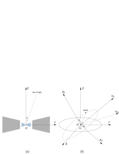
Figure 1: Panel a is a cartoon of a type I AGN with an equatorial scattering region. The blue points represent clouds in the BLR and the grey region the scatters on the equatorial plan. $i$ is the inclination angle to a remote observer in the $O-YZ$-plane. Panel b is the frame for the BLR geometry. $O-XY$ is the equatorial plane. $O-X_{\rm{}_{C}}Y_{\rm{}_{C}}$ is the orbital plane of one specific cloud, which can be obtained by rotating $X$ around $Z$ by $\phi_{\rm{}_{C}}$ and then rotating $Z$ around $X_{\rm{}_{C}}$ by $\theta_{\rm{}_{C}}$. The phase angle of the cloud relative to $OX_{\rm{}_{C}}$ is $\phi_{\rm{}_{B}}$. Panel c is the scattering geometry used here. ${\bf BP}$ is the incident light from point $B$ on one orbit. $\vec{n}_{\rm obs}$ is the direction of sight of the observer (i.e. the direction of scattered light). The vectors of $\vec{n}_{\rm obs}$, $\vec{n}_{\bot}$, $\vec{n}_{\parallel}$, $\vec{n}_{z^{\prime}}$ and $\vec{n}_{x^{\prime}}$ are explained in Appendix.

In this letter, we investigate $f_{\rm{}_{BLR}}$ in type I AGNs through modelling the scattering polarised spectra quantitatively. In section 2, we build a dynamical model for BLR and scattering region of Type I AGNs for polarized spectra. In section 3, we simulate a large number of spectra for a large range of model parameters to get the distribution of $f_{\rm{}_{BLR}}$ for both total and polarized spectra. We find that $f_{\rm{}_{BLR}}$ is in a very narrow range for polarised spectra. In section 4, we draw conclusions and discuss potential ways of improving the accuracy of BH mass determination.

2 Polarized spectra from of equatorial scatters

Optical spectropolarimetric observations of type II AGNs discover that there is a broad component of emission line in polarised spectra, indicating appearance of: 1) a BLR hidden by torus; 2) at least one scattering region outside the torus (Antonucci & Miller, 1985; Tran et al., 1992; Miller et al., 1991). Radio observations also show that radio axes of most type II AGNs are nearly perpendicular to the position angle of polarization (Antonucci, 1983; Brindle et al., 1990), showing that scattering regions of Type II AGNs situated outside the torus but aligned with the axes of the AGNs, called polar scattering region. In contrast, observations of type I AGNs reveal that position angles of the polarization are more often aligned with radio axes (Antonucci, 1983, 1984; Smith et al., 2002). Equatorial scattering regions may exist, which are hidden by the torus, but can be seen in the polarised spectra of type I AGNs (Smith et al., 2005).

We follow the geometry of equatorial scatters as in Smith et al. (2005). The geometry of the scattering regions and BLR are shown in Fig. 1a. The details of the geometric relations are provided in the Appendix. If the half opening angle of the scattering region is $\Theta_{\rm{}_{P}}$, the inner and outer radius of the scattering region is $r_{\rm{}_{P,i}}\mbox{and }r_{\rm{}_{P,o}}$, then we have $r_{\rm{}_{P}}\in[r_{\rm{}_{P,i}},r_{\rm{}_{P,o}}],\theta_{\rm{}_{P}}\in[\pi/2-\Theta_{\rm{}_{P}},\pi/2+\Theta_{\rm{}_{P}}]$. Scatterings caused by inter-cloud electrons in the BLR have been estimated as $\tau_{{}_{\rm BLR}}\approx 0.04\,R_{\rm 0.1pc}$ [see Eq. (5.13) in Krolik et al. (1981)], where $R_{\rm 0.1pc}=R_{\rm BLR}/0.1\,{\rm pc}$ is a typical size of the BLR (Bentz et al. 2013), which can be totally neglected for polarised spectra. We thus assume that the scattering region is composed of free cold electrons beyond the BLR, and the whole region is optically thin, i.e. the optical depth $\tau_{\rm es}\sim\bar{n}\ell\sigma_{\rm T}<1$, where $\bar{n}$ is the average number density of the electrons, $\ell$ is the typical scale of the region and $\sigma_{\rm T}$ is the Thomson cross section. The distribution of the number density of electrons is assumed to be a power law as $n_{\rm{}_{P}}(r_{\rm{}_{P}},\theta_{\rm{}_{P}},\phi_{\rm{}_{P}})=n_{\rm{}_{P0}}\left(r_{\rm{}_{P}}/r_{\rm{}_{P,i}}\right)^{-\alpha}$, where $n_{\rm{}_{P0}}$ is the number density at inner radius $r_{\rm{}_{P,i}}$.

We assume BLR is composed of a large quantity of independent clouds rotating around the black hole, and has a geometry indicated by Fig. 1b (Pancoast et al., 2011; Li et al., 2013; Pancoast et al., 2014a). The detailed geometric relations of BLR are given in Appendix. Suppose that the unit of length is $R_{\rm g}\equiv GM_{\bullet}/c^{2}$ and orbits of the clouds are circular. The velocity of the cloud is

$$\vec{v}_{\rm cloud}=V_{\rm K}\left(\begin{array}[]{c}-\sin\phi_{\rm{}_{B}}\cos\phi_{\rm{}_{C}}-\cos\phi_{\rm{}_{B}}\sin\phi_{\rm{}_{C}}\cos\theta_{\rm{}_{C}}\\ -\sin\phi_{\rm{}_{B}}\sin\phi_{\rm{}_{C}}+\cos\phi_{\rm{}_{B}}\cos\phi_{\rm{}_{C}}\cos\theta_{\rm{}_{C}}\\ \cos\phi_{\rm{}_{B}}\sin\theta_{\rm{}_{C}}\end{array}\right),$$ (2)

where $V_{\rm K}=cr_{{}_{\rm B}}^{-1/2}$. The half opening angle of the BLR is $\Theta_{\rm{}_{BLR}}$, the inner and outer radii of the BLR are $r_{\rm{}_{B,i}}$ and $r_{\rm{}_{B,o}}$, respectively. Then we have $r_{\rm{}_{B}}\in[r_{\rm{}_{B,i}},r_{\rm{}_{B,o}}],\theta_{\rm{}_{C}}\in[0,\Theta_{\rm{}_{BLR}}]$. The distribution of clouds can be modelled by power law as well. The number density of the clouds is $n_{\rm{}_{B}}(r_{\rm{}_{B}},\theta_{\rm{}_{C}},\phi_{\rm{}_{C}},\phi_{\rm{}_{B}})=n_{\rm{}_{B0}}\left(r_{\rm{}_{B}}/r_{\rm{}_{B,i}}\right)^{-\beta}$, where $n_{\rm{}_{B0}}$ is the number density at $r_{\rm{}_{B,i}}$.

A single scattering process is illustrated by Fig. 1c. Expressions of the scattering angle $\Theta$ and rotation angle $\chi$ are derived in Appendix. Assuming the ionizing source is isotropic and line intensity of one cloud at $B$ is linearly proportional to the intensity of local ionizing fluxes, we have the line intensity at $B$ is $i_{\rm{}_{B}}=kr_{\rm{}_{B}}^{-2}$, where $k$ is a constant. We further assume that all clouds emit unpolarized H$\beta$ photons isotropically and neglect multiple scatterings of optically thin regions. We thus have the intensity at $P$ is simply given by $i_{\rm{}_{P}}=i_{\rm{}_{B}}{\cal S}/4\pi r_{\rm{}_{BP}}^{2}$ where ${\cal S}$ is the surface area of the cloud. With incident photons with the Stokes parameters of $(i_{\rm{}_{P}},0,0,0)$, we have the Stokes parameters in the $(\vec{n}_{\bot}-\vec{n}_{\parallel})$ frame (Chandrasekhar, 1960).

$$\displaystyle{\frac{3\sigma}{8\pi R^{2}}} \!\!\!\!\!\!\!\left(\!\!\begin{array}[]{cccc}\frac{1}{2}(1+\cos^{2}\Theta)&\frac{1}{2}(1-\cos^{2}\Theta)&0&0\\ \frac{1}{2}(1-\cos^{2}\Theta)&\frac{1}{2}(1+\cos^{2}\Theta)&0&0\\ 0&0&\cos\Theta&0\\ 0&0&0&\cos\Theta\end{array}\!\!\right)\left(\!\!\begin{array}[]{c}i_{\rm{}_{P}}\\ 0\\ 0\\ 0\end{array}\!\!\right)$$ (11)

$$= {\cal A}_{0}\left(\begin{array}[]{c}1+\cos^{2}\Theta\\ 1-\cos^{2}\Theta\\ 0\\ 0\end{array}\right),$$ (16)

where ${\cal A}_{0}=3\sigma i_{\rm{}_{P}}/16\pi R^{2}$, $R$ is the distance between observer and AGN. Converting the Stokes parameter to the fixed coordinate $\vec{n}_{z^{\prime}}-\vec{n}_{x^{\prime}}$ system, we have

$$\left(\!\!\begin{array}[]{c}i\\ q\\ u\\ v\end{array}\!\!\right) = {\cal A}_{0}\left(\!\!\begin{array}[]{cccc}1&0&0&0\\ 0&\cos 2\chi&\sin 2\chi&0\\ 0&-\sin 2\chi&\cos 2\chi&0\\ 0&0&0&\cos\Theta\end{array}\!\!\right)\!\left(\!\!\begin{array}[]{c}1+\cos^{2}\Theta\\ 1-\cos^{2}\Theta\\ 0\\ 0\end{array}\!\!\right)$$ (29)

$$= {\cal A}_{0}\left(\!\!\begin{array}[]{c}1+\cos^{2}\Theta\\ (1-\cos^{2}\Theta)\cos 2\chi\\ -(1-\cos^{2}\Theta)\sin 2\chi\\ 0\end{array}\!\!\right).$$ (34)

The velocity of the cloud $\vec{v}_{\rm cloud}$ projected to the direction of incident light $\vec{n}_{\rm{}_{BP}}$ is

$$\frac{V_{\parallel}}{c}=\frac{1}{r_{\rm{}_{B}}^{1/2}}\frac{r_{\rm{}_{P}}(q_{1}\cos\phi_{\rm{}_{B}}+q_{2}\sin\phi_{\rm{}_{B}})}{[r_{\rm{}_{P}}^{2}+r_{\rm{}_{B}}^{2}+2r_{\rm{}_{B}}r_{\rm{}_{P}}(q_{2}\cos\phi_{\rm{}_{B}}-q_{1}\sin\phi_{\rm{}_{B}})]^{1/2}},$$ (35)

where $q_{1}=\cos\theta_{\rm{}_{P}}\sin\theta_{\rm{}_{C}}+\sin\theta_{\rm{}_{P}}\cos\theta_{\rm{}_{C}}\sin(\phi_{\rm{}_{P}}-\phi_{\rm{}_{C}})$, $q_{2}=-\sin\theta_{\rm{}_{P}}\cos(\phi_{\rm{}_{P}}-\phi_{\rm{}_{C}})$. If the intrinsic wavelength of the line is $\lambda_{0}$, the wavelength after scattering is $\lambda^{\prime}=\lambda_{0}(1-V_{\parallel}/c)$ due to Doppler shifts. Integrating over all the clouds and electrons, we have total polarized spectrum,

$$\left(\!\!\begin{array}[]{c}I_{\lambda}\\ Q_{\lambda}\\ U_{\lambda}\\ V_{\lambda}\end{array}\!\!\right)=\int_{V_{\rm{}_{P}}}dV_{\rm{}_{P}}n_{\rm{}_{P}}\int_{V_{\rm{}_{BLR}}}\!\!\!\!dV_{\rm{}_{BLR}}n_{\rm{}_{B}}\int_{0}^{2\pi}{\cal L}(\lambda,\lambda^{\prime})d\phi_{\rm{}_{B}}\left(\begin{array}[]{c}i\\ q\\ u\\ v\end{array}\right)$$ (36)

where the intrinsic profile of H$\beta$ line is assumed to be a Lorentzian function of ${\cal L}(\lambda,\lambda^{\prime})\propto\Gamma/[(\lambda-\lambda_{0})^{2}+\Gamma^{2}]$, $\Gamma$ is the intrinsic width much smaller than the broadening due to rotation of clouds (the Lorentzian profiles are a very good approximation in the present context).

Similarly, we can calculate the spectrum of non-scattered photons. The velocity of the cloud $\vec{v}_{\rm cloud}$ projected to the direction of observer $\vec{n}_{\rm obs}$ is

$$\frac{\tilde{V}_{\parallel}}{c}=\frac{1}{r_{\rm{}_{B}}^{1/2}}\left(\tilde{q}_{1}\cos\phi_{\rm{}_{B}}+\tilde{q}_{2}\sin\phi_{\rm{}_{B}}\right),$$ (37)

where $\tilde{q}_{1}=\sin\theta_{\rm{}_{C}}\cos i+\cos\theta_{\rm{}_{C}}\cos\phi_{\rm{}_{C}}\sin i$, $\tilde{q}_{2}=-\sin\phi_{\rm{}_{C}}\sin i$. The observed wavelength is $\lambda^{\prime\prime}=\lambda_{0}(1-\tilde{V}_{\parallel}/c)$. Integrating over all the clouds, we have

$$F_{\lambda}=\int_{V_{\rm{}_{BLR}}}dV_{\rm{}_{BLR}}n_{\rm{}_{B}}\int_{0}^{2\pi}{\cal L}(\lambda,\lambda^{\prime\prime})d\phi_{\rm{}_{B}}\frac{i_{\rm{}_{B}}S}{4\pi R^{2}},$$ (38)

and the expression for polarization degree and position angle,

$$P_{\lambda}=\frac{\sqrt{Q_{\lambda}^{2}+U_{\lambda}^{2}}}{I_{\lambda}+F_{\lambda}},\quad\theta_{\lambda}=\frac{1}{2}\arccos\left(\frac{Q_{\lambda}}{\sqrt{Q_{\lambda}^{2}+U_{\lambda}^{2}}}\right).$$ (39)

If $U_{\lambda}>0$, $\theta_{\lambda}\in(0,\pi/2)$. If $U_{\lambda}<0$, $\theta_{\lambda}\in(-\pi/2,0)$. Position angles represent the angle between the direction of maximum intensity and $n_{z^{\prime}}$.

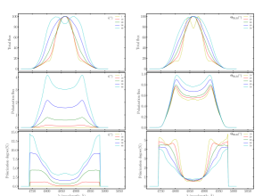
Figure 2: Total, polarised spectra and polarisation degrees of a type I AGN with an equatorial electron scattering region. The left column are spectra for different inclinations whereas the right for different BLR opening angles. The tops of the total spectra become flatter and polarisation decreases with increases $\Theta_{\rm BLR}$ (tends to $90^{\circ}$).

Table 1 summarises all the parameters of the present model. We calculate a series of profiles for different values of parameters and find that the profiles are only sensitive to $\Theta_{{}_{\rm BLR}}$ and $i$. Fig. 2 shows typical spectra of a type I AGN with an equatorial electron scattering region. The parameters of the model are $r_{\rm{}_{P,i}}=10^{4}$, $r_{\rm{}_{P,o}}=2\times 10^{4}$, $\Theta_{\rm{}_{P}}=30^{\circ}$, $r_{\rm{}_{B,i}}=2\times 10^{3}$, $r_{\rm{}_{B,o}}=6\times 10^{3}$, $\alpha=1$, $\beta=1$, $\tau_{\rm es}=\sigma n_{\rm{}_{P0}}(r_{\rm{}_{P,o}}-r_{\rm{}_{P,i}})=1$, $i=(1^{\circ},10^{\circ},20^{\circ},30^{\circ},40^{\circ})$ and $\Theta_{{}_{\rm BLR}}=(10^{\circ},20^{\circ},30^{\circ},40^{\circ},50^{\circ})$. As shown by the left panel of Fig. 2, the total spectra get broader as $i$ increases and show double peaked-profiles when $i$ exceeds a critical inclination. By contrast, the width and the profile of the polarised spectra are not sensitive to $i$ (can be found from normalized spectra). This interesting property results from the fact that the polarised spectra are equivalent to the ones seen by observers at edge-on orientations. Generally, the line centres have lowest polarisation degrees. However, polarization degrees become smaller with $i$.

Total spectra show strong dependence on $\Theta_{\rm BLR}$. As shown in the right panel of Fig. 2, large-$\Theta_{\rm BLR}$ BLRs show broader width and get narrower with decreases of $\Theta_{\rm BLR}$ until double peaked-profiles. However, $\Theta_{{}_{\rm BLR}}$ does not change the polarised profiles too much. Large $\Theta_{{}_{\rm BLR}}$ indicates that the system tends to be more spherically symmetric and to decrease the polarization degree. Comparing with the total spectra, the width of the polarised spectrum is insensitive to $\Theta_{{}_{\rm BLR}}$ and $i$. This property allows us to infer $f_{\rm{}_{BLR}}$ from the polarized spectrum and improve the accuracy of BH mass measurement as shown in §3.

3 The virial factor

With the BLR model, we have the emissivity-averaged time lag of broad emission line as

$$\Delta t=\frac{\int dV_{\rm{}_{BLR}}\Delta ri_{\rm{}_{B}}n_{\rm{}_{B}}}{\int dV_{\rm{}_{BLR}}i_{\rm{}_{B}}n_{\rm{}_{B}}}\left(\frac{R_{\rm g}}{c}\right)=\frac{1-\beta}{2-\beta}\frac{1-q_{r}^{2-\beta}}{1-q_{r}^{1-\beta}}\left(\frac{r_{{}_{\rm B,i}}R_{\rm g}}{c}\right),$$ (40)

where $\Delta r=r_{\rm{}_{B}}-\vec{r}_{\rm{}_{B}}\cdot\vec{n}_{\rm obs}$ and the corresponding virial factor from Eq. (1) can be written as

$$f_{\rm{}_{BLR}}^{-1}=\left(\frac{1-\beta}{2-\beta}\right)\left(\frac{1-q_{r}^{1-\beta}}{1-q_{r}^{2-\beta}}\right)\left(\frac{V_{\rm{}_{FWHM}}}{c}\right)^{2}r_{{}_{\rm B,i}},$$ (41)

where $q_{r}=r_{{}_{\rm B,o}}/r_{{}_{\rm B,i}}$, $V_{{}_{\rm FWHM}}$ is FWHM of profiles either from the total or polarised spectra. We generate profiles according to parameters listed in Table 1 and measure $V_{{}_{\rm FWHM}}$ to show dependences of $f_{\rm{}_{BLR}}$ on each parameter.

We did Monte-Carlo simulations for all the parameters listed in Table 1 and then get the $\ln f_{\rm{}_{BLR}}-\ln X_{i}$ relations, where $X_{i}$ is any one of the parameters. The $f_{\rm{}_{BLR}}$-dependence on $X_{i}$ can then be obtained by $\delta\ln f_{\rm{}_{BLR}}=\left(\partial\ln f_{\rm{}_{BLR}}/\partial\ln X_{i}\right)\delta\ln X_{i}$, where $\partial\ln f_{\rm{}_{BLR}}/\partial\ln X_{i}$ is the slope of the $\ln f_{\rm{}_{BLR}}-\ln X_{i}$ relations, $\delta\ln X_{i}$ is its range. The slope is estimated from the line regression of $\ln f_{\rm{}_{BLR}}-\ln X_{i}$ relations from the Monte-Carlo simulations. Dependence listed in Table 1 shows that only $i$ and $\Theta_{\rm BLR}$ are the major drivers in the total spectra, but $f_{\rm{}_{BLR}}$ is insensitive to all the parameters (only slightly relies on $\Theta_{\rm BLR}$). We estimate the entire uncertainties of $f_{\rm{}_{BLR}}$ due to all parameters as $\Delta\log f_{\rm{}_{BLR}}=\left[\sum_{i=1}^{9}(\partial\ln f_{\rm{}_{BLR}}/\partial\ln X_{i})^{2}\left(\Delta\log X_{i}\right)^{2}\right]^{1/2}$. We have $\Delta\log f_{\rm{}_{BLR}}=(0.74,0.04)$ for total and polarised spectra, respectively.

We plot the $\log f_{\rm{}_{BLR}}-$distributions and contour maps versus $\Theta_{\rm BLR}$ and $i$ in Fig. 3. It shows that the distribution from total spectra is much broader than that from polarised spectra. The $68\%$ confidence interval of the former is $\log f_{\rm{}_{BLR}}\in[-0.41,0.08]$ agreeing with values from detailed MCMC modelling (Pancoast et al., 2014b), but $\log f_{\rm{}_{BLR}}\in[-0.65,-0.62]$ from the polarised spectra. For a typical RM campaign, we have the uncertainties of BH mass $\delta M_{\bullet}/M_{\bullet}\approx(0.8,0.3)$ from total and polarised spectra, respectively. Obviously, spectropolarimetry provides much better $f_{\rm{}_{BLR}}$ for BH mass from RM campaign. However, the polarised spectra as the prerequisites of applications should be identified as originating from the equatorial scatters. Actually, this can be done by checking if the position angles are parallel to radio axis in AGNs.

We apply the current $f_{\rm{}_{BLR}}$ to the radio-loud narrow line Seyfert 1 galaxy PKS 2004$-$447 with $V_{\rm FWHM}({\rm H\alpha})=1500\,\rm km\,s^{-1}$($z=0.240$). The black hole mass estimated by single total spectra is about $5\times 10^{6}M_{\odot}$ (Oshlack et al., 2001), which is much smaller than the critical mass ($M_{\bullet}\sim 10^{8}M_{\odot}$) invariably associated with classical radio load(RL) AGNs(Laor, 2000). Fortunately, the polarised spectra of VLT observations show its $\rm H\alpha$ FWHM of $(280\pm 50)$Å (Baldi et al., 2016). Since the 5100Å  luminosity is $L_{5100}=1.25\times 10^{44}\rm erg\,s^{-1}$ (Gallo et al., 2006), $R-L$ relation indicates that the average time lag between emission line and continuum is about $10^{1.6\pm 0.14}$ days (Bentz et al., 2013) for sub-Eddington AGNs (Du et al., 2016). Taking $\log f_{\rm{}_{BLR}}=-0.63$ for the polarised spectra of H$\alpha$ line, we have $M_{\bullet}=10^{8.45\pm 0.2}M_{\odot}$. Employing the standard accretion disk model, we have the dimensionless accretion rates of $\dot{\mathscr{M}}=\dot{M}c^{2}/L_{\rm Edd}=20.1\left(L_{44}/\cos i\right)^{3/2}m_{7}^{-2}\approx 0.05$, where $\dot{M}$ is the accretion rates, $L_{\rm Edd}=1.4\times 10^{38}\left(M_{\bullet}/M_{\odot}\right)\rm erg\,s^{-1}$, $L_{44}=L_{5100}/10^{44}\rm erg\,s^{-1}$, $\cos i=0.75$ (inclination) and $m_{7}=M_{\bullet}/10^{7}M_{\odot}$ (Du et al., 2014). Such a low accretion rate agrees with the radio-loudness and accretion rate relation (Sikora et al., 2007).

Finally, we would like to point out the temporal properties of polarised spectra. The equatorial distributions of scatters lead to delays of polarised photons with different frequencies relative to the BLR, and such a delay may need to be considered for polarised spectra at different epochs. Such a kind of polarisation campaigns will provide a new way of accurately measuring the black hole mass in type 1 AGNs.

Table 1: The dependence of $f_{\rm{}_{BLR}}$ on model parameters                                                                                      

Parameter	Range	Meaning	$\delta\ln f_{{}_{\rm BLR}}$
			total	polarized
$r_{\rm{}_{P,i}}(10^{4}R_{\rm g})$	$[1,5]$	SR inner radius	$0.01$	$0$
$r_{\rm{}_{P,o}}(10^{4}R_{\rm g})$	$[2,10]$	SR outer radius	$0$	$0$
$\Theta_{\rm{}_{P}}(^{\circ})$	$[20,50]$	SR opening angle	$-0.04$	$0$
$\alpha$	$[0,1.5]$	index of DF of electrons	$0.01$	$0$
$r_{\rm{}_{B,i}}(10^{3}R_{\rm g})$	$[1,5]$	inner radius of BLR	$-0.01$	$0.01$
$r_{\rm{}_{B,o}}(10^{3}R_{\rm g})$	$[2,10]$	outer radius of BLR	$0.01$	$-0.01$
$\Theta_{\rm{}_{BLR}}(^{\circ})$	$[20,50]$	opening angle of BLR	$-0.38$	$0.03$
$\beta$	$[0,1.5]$	index of DF of clouds	$0$	$-0.02$
$i(^{\circ})$	$[0,45]$	inclination angle	$-0.64$	$0$

Note. — SR: scattering region, DF: distribution function. $\delta\ln f_{\rm{}_{BLR}}$ describes the dependence on parameters of the broad-line regions. See details for its definition in the main text. It shows that $f_{\rm{}_{BLR}}$ is sensitive to $\Theta_{\rm BLR}$ and $i$ for the total spectra, but it is almost a constant for polarised spectra.

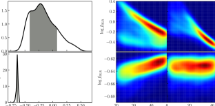
Figure 3: The upper three panels display the distribution of $\log f_{\rm{}_{BLR}}$ obtained from total spectra while the lower three polarized spectra. In each row, the first panel is the probability density function of $\log f_{\rm{}_{BLR}}$ and the shadow area marks out the $68\%$ confidence interval, the second and third indicate correlations of $\log f_{\rm{}_{BLR}}$ with model parameters of $\Theta_{\rm{}_{BLR}}$ and $i$, respectively. $f_{\rm{}_{BLR}}$ is sensitive to both $\Theta_{\rm BLR}$ and $i$ for the total spectra whereas $f_{\rm{}_{BLR}}$ only very weakly depends on $\Theta_{\rm BLR}$.

4 Conclusion and Discussion

In this Letter, we show that the factor $f_{\rm BLR}$ has a wide range for total spectra of the virialized the broad-line regions. We investigate the polarised spectra of the BLR arisen from the equatorial scatters for $f_{\rm{}_{BLR}}$ in determination of black hole mass in type I AGNs. It is found that $\log f_{\rm{}_{BLR}}\in[-0.65,-0.62]$ for polarised spectra. This arises from the fact that the electrons on the equatorial plane scatter the broad-line photons to observers, assembling to view the BLR as edge-on orientation. The polarised spectra provide a way of accurately measuring BH mass from single epoch polarised spectra, which is much better than that from single epoch total spectra. For an individual application, equatorial scatters must be checked for the validity of the polarised spectra.

We note the work of Afanasiev & Popović (2015), who employed the angles of polarisation arisen by scatters on the inner edge of the dusty torus in order to alleviate dependence of black hole mass on inclinations. This is different from what we suggest in this paper. We would like to point out the major assumptions used in this paper that scattering region is equatorial, but static. The geometry of scatters is supported by observations but the dynamics could be more complicated. We also neglect scatters of dust particles. This simple model shows the potential functions of polarised spectra in measuring black hole mass. Fitting the polarised spectra leads to more accurate BH mass, but we will conduct it in a forthcoming paper.

Appendix

For type I AGN, the polarised spectra observed by a remote observer are mostly caused by electron scattering of the equatorial regions. Suppose the coordinate of the electron in spherical system is $(r_{\rm{}_{P}}$, $\theta_{\rm{}_{P}}$, $\phi_{\rm{}_{P}})$, we have

$$\begin{cases}x_{\rm{}_{P}}=r_{\rm{}_{P}}\sin\theta_{\rm{}_{P}}\cos\phi_{\rm{}_{P}},\\ y_{\rm{}_{P}}=r_{\rm{}_{P}}\sin\theta_{\rm{}_{P}}\sin\phi_{\rm{}_{P}},\\ z_{\rm{}_{P}}=r_{\rm{}_{P}}\cos\theta_{\rm{}_{P}}.\end{cases}$$ (42)

As for a cloud in BLR at $(r_{\rm{}_{B}}\cos\phi_{\rm{}_{B}},r_{\rm{}_{B}}\sin\phi_{\rm{}_{B}},0)$, we use the rotation matrix

$$\mathbf{R}=\left(\begin{array}[]{ccc}\cos\phi_{\rm{}_{C}}&-\sin\phi_{\rm{}_{C}}\cos\theta_{\rm{}_{C}}&\sin\phi_{\rm{}_{C}}\sin\theta_{\rm{}_{C}}\\ \sin\phi_{\rm{}_{C}}&\cos\phi_{\rm{}_{C}}\cos\theta_{\rm{}_{C}}&-\cos\phi_{\rm{}_{C}}\sin\theta_{\rm{}_{C}}\\ 0&\sin\theta_{\rm{}_{C}}&\cos\theta_{\rm{}_{C}}\end{array}\right),$$ (43)

for the position of the cloud

$$\begin{cases}x_{\rm{}_{B}}=r_{\rm{}_{B}}(\cos\phi_{\rm{}_{B}}\cos\phi_{\rm{}_{C}}-\sin\phi_{\rm{}_{B}}\sin\phi_{\rm{}_{C}}\cos\theta_{\rm{}_{C}}),\\ y_{\rm{}_{B}}=r_{\rm{}_{B}}(\cos\phi_{\rm{}_{B}}\sin\phi_{\rm{}_{C}}-\sin\phi_{\rm{}_{B}}\cos\phi_{\rm{}_{C}}\cos\theta_{\rm{}_{C}}),\\ z_{\rm{}_{B}}=r_{\rm{}_{B}}\sin\theta_{\rm{}_{C}}\sin\phi_{\rm{}_{B}},\end{cases}$$ (44)

in the $O-XYZ$ frame.

One cloud is at $(x_{\rm{}_{B}},y_{\rm{}_{B}},z_{\rm{}_{B}})$ and one scattering electron is at $(x_{\rm{}_{P}},y_{\rm{}_{P}},z_{\rm{}_{P}})$, we have the direction vector of incident light

$$\vec{n}_{\rm{}_{BP}}=\frac{1}{r_{\rm{}_{BP}}}\left[(x_{\rm{}_{P}}-x_{\rm{}_{B}})\vec{i}+(y_{\rm{}_{P}}-y_{\rm{}_{B}})\vec{j}+(z_{\rm{}_{P}}-z_{\rm{}_{B}})\vec{k}\right],$$ (45)

where $r_{\rm{}_{BP}}=\sqrt{(x_{\rm{}_{P}}-x_{\rm{}_{B}})^{2}+(y_{\rm{}_{P}}-y_{\rm{}_{B}})^{2}+(z_{\rm{}_{P}}-z_{\rm{}_{B}})^{2}}$. The direction of the observer at infinity is taken to be $\vec{n}_{\rm obs}=(0,\sin i,\cos i)$. The scattering angle is given by

$$\cos\Theta=\vec{n}_{\rm obs}\cdot\vec{n}_{\rm{}_{BP}}=\frac{1}{r_{\rm{}_{BP}}}\left[(y_{\rm{}_{P}}-y_{\rm{}_{B}})\sin i+(z_{\rm{}_{P}}-z_{\rm{}_{B}})\cos i\right].$$ (46)

The unit vector perpendicular to the scattering plane is

$$\vec{n}_{\bot}=\frac{\vec{n}_{\rm{}_{BP}}\times\vec{n}_{\rm obs}}{|\vec{n}_{\rm{}_{BP}}\times\vec{n}_{\rm obs}|}.$$ (47)

We take the fixed coordinate system at celestial sphere of the observer to be $\vec{n}_{z^{\prime}}-\vec{n}_{x^{\prime}}$, $\vec{n}_{z^{\prime}}=(0,-\cos i,\sin i),\vec{n}_{x^{\prime}}=(1,0,0)$. The angle between $\vec{n}_{\bot}$ and $\vec{n}_{z^{\prime}}$ satisfies that

$$\cos\chi=\frac{x_{{}_{\rm P}}-x_{{}_{\rm B}}}{\left\{[(z_{\rm{}_{P}}-z_{\rm{}_{B}})\sin i-(y_{\rm{}_{P}}-y_{\rm{}_{B}})\cos i]^{2}+(x_{\mathrm{P}}-x_{\mathrm{B}})^{2}\right\}^{1/2}}.$$ (48)

References

- Afanasiev & Popović (2015) Afanasiev V. L., Popović L. C., 2015, ApJ, 800, L35
- Antonucci (1983) Antonucci R. R., 1983, Nature, 303, 158
- Antonucci (1984) Antonucci R., 1984, ApJ, 278, 499
- Antonucci & Miller (1985) Antonucci R., Miller J., 1985, ApJ, 297, 621
- Baldi et al. (2016) Baldi R. D., Capetti A., Robinson A., Laor A., Behar E., 2016, MNRAS, 458, L69
- Barth et al. (2016) Barth A. J., Boizelle B. D., Darling J., Baker A. J., Buote D. A., Ho L. C., Walsh J. L., 2016, ApJ, 822, L28
- Bentz et al. (2013) Bentz M. C., et al., 2013, ApJ, 767, 149
- Brindle et al. (1990) Brindle C., Hough J., Bailey J. et al. 1990, MNRAS, 244, 577
- Chandrasekhar (1960) Chandrasekhar S., 1960, Radiative Transfer. New York: Dover
- Collin et al. (2006) Collin S., Kawaguchi T., Peterson B. M., Vestergaard M., 2006, A&A, 456, 75
- Du et al. (2014) Du P., et al., 2014, ApJ, 782, 45
- Du et al. (2016) Du P., et al., 2016, ApJ, 825, 126
- Du et al. (2017) Du P., Wang J.-M., Zhang Z.-X., 2017, ApJ, 840, L6
- Gallo et al. (2006) Gallo L., et al., 2006, MNRAS, 370, 245
- Ho & Kim (2014) Ho L. C., Kim M., 2014, ApJ, 789, 17
- (16) Krolik, J. H., McKee, C. F. and Tarter, C. B. 1981, ApJ, 249, 422
- Krolik et al. (1981) Krolik J., McKee C. F., Tarter C., 1981, ApJ, 249, 422
- Krolik (2001) Krolik J. H., 2001, ApJ, 551, 72
- Laor (2000) Laor A., 2000, ApJ, 543, L111
- Li et al. (2013) Li Y.-R., Wang J.-M., Ho L. C., Du P., Bai J.-M., 2013, ApJ, 779, 110
- Miller et al. (1991) Miller J., Goodrich R., Mathews W. G., 1991, ApJ, 378, 47
- Miyoshi et al. (1995) Miyoshi M., Moran J., Herrnstein J., Greenhill L., Nakai N., Diamond P., Inoue M., 1995, Nature, 373, 127
- Onken et al. (2004) Onken C. A., Ferrarese L., Merritt D., Peterson B. M., Pogge R. W., Vestergaard M., Wandel A., 2004, ApJ, 615, 645
- Oshlack et al. (2001) Oshlack A., Webster R., Whiting M., 2001, ApJ, 558, 578
- Pancoast et al. (2011) Pancoast A., Brewer B. J., Treu T., 2011, ApJ, 730, 139
- Pancoast et al. (2014a) Pancoast A., Brewer B. J., Treu T., 2014a, MNRAS, 445, 3055
- Pancoast et al. (2014b) Pancoast A., Brewer B. J., Treu T., Park D., Barth A. J., Bentz M. C., Woo J.-H., 2014b, MNRAS, 445, 3073
- Peterson (1993) Peterson B. M., 1993, Publ. Astron. Soc. Australia, 105, 247
- Peterson (2014) Peterson B. M., 2014, Space Sci. Rev., 183, 253
- Sikora et al. (2007) Sikora M., Stawarz Ł., Lasota J.-P., 2007, ApJ, 658, 815
- Smith et al. (2002) Smith J., Young S., Robinson A., Corbett E., Giannuzzo M., Axon D., Hough J., 2002, MNRAS, 335, 773
- Smith et al. (2005) Smith J., Robinson A., Young S., Axon D., Corbett E. A., 2005, MNRAS, 359, 846
- Tran et al. (1992) Tran H. D., Miller J. S., Kay L. E., 1992, ApJ, 397, 452
- Woo et al. (2010) Woo J.-H., et al., 2010, ApJ, 716, 269