Superfluid transition temperature of spin-orbit and
Rabi coupled fermions with tunable interactions

Abstract

We obtain the superfluid transition temperature of equal Rashba-Dresselhaus spin-orbit and Rabi coupled Fermi superfluids, from the Bardeen-Cooper-Schrieffer (BCS) to Bose-Einstein condensate (BEC) regimes in three dimensions. Spin-orbit coupling enhances the critical temperature in the BEC limit, and can convert a first order phase transition in the presence of Rabi coupling into second order, as a function of the Rabi coupling for fixed interactions. We derive the Ginzburg-Landau equation to sixth power in the superfluid order parameter to describe both first and second order transitions as a function of spin-orbit and Rabi couplings.

The ability to simulate magnetic fields in cold atoms systems opens the possibility of exploring new physics unachievable elsewhere. In addition to artificial Abelian magnetic fields Lin2009 ; Lin2009-2 ; Ketterle2015 , one can also generate non-Abelian fields in both bosonic and fermionic systems Lin2011 ; zwierlein2012 ; wang2012 ; Spielman2013 ; Galitski2013 ; Zhang2014 ; fallani2015 ; huang2016 ; wu2016 . The latter will eventually lead to the possibility of simulating quantum chromodynamics lattice gauge theory cirac2012 ; Wiese-2013 ; Zohar2015 ; Dalmonte2016 . Present experiments on three dimensional spin-orbit coupled Fermi gases are still at too high a temperature for these systems to undergo Bardeen-Cooper-Schrieffer (BCS) pairing, because the current Raman scheme causes heating. In contrast, theory has concentrated at zero temperature Zhang2011 ; Zhai2011 ; Pu2011 ; Han2012 ; Seo2012a ; Seo2012b . Once such fermionic systems can be cooled below the superfluid transition temperature, the spin-orbit coupling is expected to reveal new states with non-conventional pairing. Even weak spin orbit coupling will produce an admixture of s-wave and p-wave pairing.

In this Letter, we investigate the transition temperature of Fermi superfluids with an equal mixture of Rashba and Dresselhaus spin-orbit coupling as a function of the Rabi coupling, throughout the entire BCS (Bardeen-Cooper-Schrieffer)-to-BEC (Bose-Einstein condensation) evolution in three dimensions; the single particle Hamiltonian matrix is

$${\bf H}_{so}(\hat{\bf p})=\frac{(\hat{p}_{x}-\kappa\sigma_{y})^{2}}{2m}+\frac{\hat{p}_{y}^{2}}{2m}+\frac{\hat{p}_{z}^{2}}{2m}-\frac{\Omega}{2}\sigma_{z};$$ (1)

the Pauli sigma matrices operate in the two-level space, $\hat{\bf p}$ is the momentum, $\Omega$ is the Rabi frequency, and $\kappa$ is the momentum transfer to the atoms in a two-photon Raman process Spielman2013 . This problem bears a close relation to spin-orbit coupling in solids, where the coupling $\sim p_{i}\sigma_{j}$ is intrinsic, and where the role of the Rabi frequency is played by an external Zeeman magnetic field. While a mean field treatment describes well the evolution from the BCS to the BEC regime at zero temperature Leggett1980 , this order of approximation fails to describe the correct critical temperature of the system in the BEC regime, because the physics of two-body bound states (Feshbach molecules) Carlos1993 is not captured when the pairing order parameter goes to zero. To remedy this problem, we include effects of order-parameter fluctuations in the thermodynamic potential.

We stress that our present results are applicable to both neutral cold atomic and charged condensed matter systems. We find that the spin-orbit coupling can enhance the critical temperature of the superfluid in the BEC regime and that it can convert a discontinuous first order phase transition in the presence of Rabi coupling into a continuous second order transition, as a function of the Rabi frequency (or Zeeman field in solids) for fixed interactions. We analyze the nature of the phase transition in terms of the Ginzburg-Landau free energy, calculating it to six powers of the superfluid order parameter to allow for the description of continuous and discontinuous transitions as a function of the spin-orbit coupling, Rabi frequency, and interactions.

To describe three dimensional Fermi superfluids in the presence of spin-orbit and Zeeman fields, we start from the Hamiltonian density

$${\cal H}({\bf r})={\cal H}_{so}({\bf r})+{\cal H}_{I}({\bf r}),$$ (2)

and use units $\hbar=k_{B}=1$. The first term in Eq. (2) is the independent-particle contribution including spin-orbit coupling,

$${\cal H}_{so}({\bf r})=\sum_{ss^{\prime}}\psi^{\dagger}_{s}({\bf r})\left[{\bf H}_{so}({\hat{\bf p}})\right]_{ss^{\prime}}\psi_{s^{\prime}}({\bf r}),$$ (3)

The second term describes the two-body s-wave contact interaction

$${\cal H}_{I}({\bf r})=-g\psi^{\dagger}_{\uparrow}({\bf r})\psi^{\dagger}_{\downarrow}({\bf r})\psi_{\downarrow}({\bf r})\psi_{\uparrow}({\bf r}),$$ (4)

where the arrows indicate the pseudospins of the fermions, which we refer to simply as “spins”. Here $g>0$ corresponds to a constant attraction between opposite spins.

The pairing field $\Delta({\bf r},\tau)=-g\langle\psi_{\downarrow}({\bf r},\tau)\psi_{\uparrow}({\bf r},\tau)\rangle$ describes the formation of pairs of two fermions with opposite  spins, where $\tau=it$ is the imaginary time. Standard manipulations lead to the Lagrangian density

$${\cal L}({\bf r,\tau}) = \frac{1}{2}\hskip 1.42262pt\Psi^{\dagger}({\bf r},\tau){\bf G}^{-1}({\bf r},\tau)\Psi({\bf r},\tau)+\frac{|\Delta({\bf r},\tau)|^{2}}{g}$$ (5)

$$\hskip 14.22636pt+K({\bf r})\delta({\bf r}-{\bf r}^{\prime}),$$

where $\Psi=(\psi_{\uparrow}\hskip 2.84526pt\psi_{\downarrow}\hskip 2.84526pt\psi^{\dagger}_{\uparrow}\hskip 2.84526pt\psi^{\dagger}_{\downarrow})^{T}$ is the Nambu spinor, and $K\equiv-\nabla^{2}/2m-\mu$ is the kinetic energy operator measured with respect to the fermion chemical potential $\mu$. We note that the definition of $\mu$ already includes the overall positive shift $\kappa^{2}/2m$ in the single particle kinetic energies due to spin-orbit coupling, that is, $\mu$ is measured with respect to $\kappa^{2}/2m$.

The inverse Green’s function appearing in Eq. (5) is

$${\bf G}_{\bf k}^{-1}(\tau)=\begin{pmatrix}\partial_{\tau}-K_{\uparrow}&-i\kappa k_{x}/m&0&-\Delta\\ i\kappa k_{x}/m&\partial_{\tau}-K_{\downarrow}&\Delta&0\\ 0&\Delta^{*}&\partial_{\tau}+K_{\uparrow}&-i\kappa k_{x}/m\\ -\Delta^{*}&0&i\kappa k_{x}/m&\partial_{\tau}+K_{\downarrow}\end{pmatrix},$$

(6)

where $K_{\uparrow}=K-\Omega/2,$ and $K_{\downarrow}=K+\Omega/2$ are the kinetic energy terms shifted by the Rabi coupling. As mentioned above, the mean field treatment fails to describe the correct critical temperature of the system in the BEC regime. To incorporate the physics of two-body bound states, we must include effects of order-parameter fluctuations in the thermodynamic potential.

To obtain the transition temperature to the superfluid state, we analyze the partition function ${\cal Z}$ as a functional integral $\int{\cal D}\Delta{\cal D}\Delta^{*}\int{\cal D}\Psi{\cal D}\Psi^{\dagger}e^{\cal S}$ for the Fermi superfluid, where ${\cal S}=\int_{0}^{\beta}\int d^{3}{\bf r}{\cal L}({\bf r},\tau)$ is the full action of the system. Upon integration over the fermion fields, the thermodynamic potential $\Omega=-T\ln{\cal Z}$ contains two terms $\Omega=\Omega_{0}+\Omega_{F}$, where $\Omega_{0}=-T\ln{\cal Z}_{0}=-TS_{0}$ is the saddle point contribution, at which point $\Delta({\bf r},\tau)=\Delta_{0}$, and $\Omega_{F}=-T\ln{\cal Z}_{F}$ is the fluctuation part. The subscript $0$ denotes quantities calculated in mean field.

The mean-field (saddle-point) term in the thermodynamic potential is

$$\Omega_{0}=V\frac{|\Delta_{0}|^{2}}{g}-\frac{T}{2}\sum_{{\bf k},j}\ln\left[1+e^{-\beta E_{j}({\bf k})}\right]+\sum_{\bf k}\xi_{k},$$ (7)

where $\xi_{k}=\varepsilon_{k}-\mu$, $\varepsilon_{k}={k}^{2}/2m$, and the $E_{j}({\bf k})$ are the eigenvalues of the Nambu Hamiltonian matrix ${\bf H}_{0}({\bf k})={\bf 1}\partial_{\tau}-{\bf G}_{\bf k}^{-1}(\tau)$, with $j=\{1,2,3,4\}$. The first set of eigenvalues

$$E_{1,2}({\bf k})=\sqrt{E_{0,k}^{2}+h_{\bf k}^{2}\pm 2\sqrt{E_{0,k}^{2}+h_{\bf k}^{2}-|\Delta_{0}|^{2}(\kappa k_{x}/m)^{2}}},$$ (8)

describe quasiparticle excitations, and the second set of eigenvalues $E_{3,4}({\bf k})=-E_{1,2}({\bf k})$ correspond to quasiholes. Here $E_{0,k}=\sqrt{\xi^{2}_{k}+|\Delta_{0}|^{2}},$ and $h_{\bf k}\equiv\sqrt{(\kappa k_{x}/m)^{2}+\Omega^{2}/4}$ is the magnitude of the combined spin-orbit and Rabi couplings.

The order parameter equation is found from the saddle point condition $\delta\Omega_{0}/\delta\Delta_{0}^{*}|_{T,V,\mu}=0$, leading to

$$\frac{m}{4\pi a_{s}}=\frac{1}{2V}\sum_{\bf k}\bigg{[}\frac{1}{\varepsilon_{k}}-A_{+}-\frac{h^{2}_{z}}{\xi_{k}h_{\bf k}}\hskip 1.42262ptA_{-}\bigg{]}.$$ (9)

Here, we write the interaction $g$ in terms of the renormalized $s$-wave scattering length $a_{s}$ via the relation $1/g=-m/4\pi a_{s}+(1/V)\sum_{\bf k}1/2\varepsilon_{k}$  as_note ; Goldbart2011 ; Ozawa2012 , and for short write $A_{\pm}=(1-2n_{{\bf k},1})/2E_{1}\pm(1-2n_{{\bf k},2})/2E_{2},$ with $n_{{\bf k},i}=1/(e^{\beta E_{{\bf k},i}}+1)$ the Fermi function. In addition, the particle number at the saddle point $N_{0}=-\partial\Omega_{0}/\partial\mu|_{T,V},$ is given by

$$N_{0}=\sum_{\bf k}\bigg{\{}1-\xi_{k}\bigg{[}A_{+}+\frac{(\kappa k_{x}/m)^{2}}{\xi_{k}h_{\bf k}}\hskip 1.42262ptA_{-}\bigg{]}\bigg{\}}.$$ (10)

The saddle point transition temperature $T_{0}$ is determined by solving Eq. (9) for given $\mu$. The corresponding number of particles is given by Eq. (10). This mean field treatment leads to a transition temperature growing as $e^{1/k_{F}a_{s}}$ for $k_{F}a_{s}\to 0^{+}$. To find the physically correct transition temperature we must, in constructing the thermodynamic potential, include the physics of two-body bound states near the transition via the two-particle t-matrix  Nozieres1985 ; Baym2006 . With all the two particle channels taken into account, the t-matrix calculation leads to a two-particle scattering amplitude, $\Gamma$, where

$$\Gamma^{-1}({\bf q},z)=\frac{m}{4\pi a_{s}}-\frac{1}{2V}\sum_{\bf k}\bigg{[}\frac{1}{~{}\varepsilon_{k}}+\sum^{2}_{i,j=1}\alpha_{ij}W_{ij}\bigg{]};$$ (11)

here $z$ is the (complex) frequency, $W_{ij}=(1-n_{{\bf k},i}-n_{{\bf k+q},j})/(z-E_{i}({\bf k})-E_{j}({\bf k+q})).$ In the limit that the order parameter goes to 0, the single particle eigenvalues reduce to $E_{1,2}({\bf k})=\xi_{k}\pm h_{\bf k}$ eigenvalue_note . The coefficients $\alpha_{11}=\alpha_{22}=|u_{\bf k}u_{{\bf k}+{\bf q}}-v_{\bf k}v^{*}_{{\bf k}+{\bf q}}|^{2}$ and $\alpha_{12}=\alpha_{21}=|u_{\bf k}v_{{\bf k}+{\bf q}}+u_{{\bf k}+{\bf q}}v_{\bf k}|^{2}$ are weighting functions of the amplitudes

$$u_{\bf k}=\sqrt{\frac{1}{2}\left(1+\frac{\Omega}{2h_{\bf k}}\right)},\hskip 14.22636ptv_{\bf k}=i\sqrt{\frac{1}{2}\left(1-\frac{\Omega}{2h_{\bf k}}\right)}.$$ (12)

As the fermion chemical potential becomes large and negative, the system becomes non-degenerate and $\Gamma^{-1}({\bf q},z)=0$ becomes the exact eigenvalue equation for the two-body bound state in the presence of spin-orbit and Rabi coupling Doga2016 . The solution is $z=E_{bs}({\bf q})-2\mu$, where $E_{bs}(\bf q)$ is the two-body bound state energy. The fluctuation correction to the thermodynamic potential is then $\Omega_{F}=-T\sum_{{\bf q},iq_{n}}\ln\left[\beta\Gamma({\bf q},iq_{n})/V\right].$

From $\Omega_{F}$ we obtain the fluctuation contribution to the particle number $N_{F}=-\partial\Omega_{F}/\partial\mu|_{T,V}=N_{sc}+N_{b}$. Here,

$$N_{sc}=\sum_{\bf q}\int^{\infty}_{\omega_{tp}({\bf q})}\frac{d\omega}{\pi}n_{B}(\omega)\left[\frac{\partial\delta({\bf q},\omega)}{\partial\mu}-\frac{\partial\delta({\bf q},0)}{\partial\mu}\right]_{V,T}$$ (13)

is the number of particles in scattering states, where the phase shift $\delta({\bf q},\omega)$ is defined via the relation $\Gamma({\bf q},\omega\pm i\epsilon)=|\Gamma({\bf q},\omega)|e^{\pm i\delta({\bf q},\omega)}$ and $\omega_{tp}({\bf q})$ is the two-particle continuum threshold corresponding to the branch point of $\Gamma^{-1}({\bf q},z)$ Nozieres1985 ; Pethick2011 . Also,

$$N_{b}=2\sum_{\bf q}n_{B}(E_{bs}({\bf q})),$$ (14)

is the number of fermions in bound states with $n_{B}(\omega)=1/(e^{\beta\omega}-1)$ the Bose distribution function. The total number of fermions, as a function of $\mu$, becomes

$$N=N_{0}+N_{F},$$ (15)

where $N_{0}$ is given in Eq. (10) and $N_{F}$ is the sum the two contributions $N_{sc}$ and $N_{b}$ discussed above Nozieres1985 ; Carlos1993 .

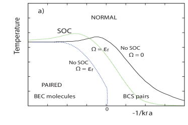
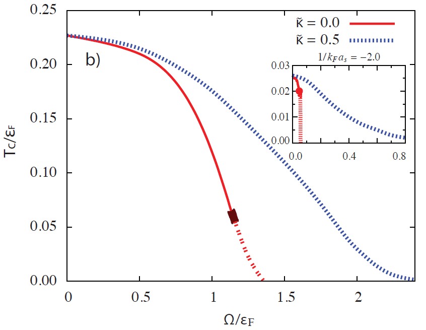
Figure 1: (Color online) a) The transition temperature $T_{c}$ for ERD spin-orbit coupling for two Rabi coupling strengths, $\Omega=0$ and $\varepsilon_{F}$. For $\Omega=0$, solid (black) curve, $T_{c}$ is that for zero spin-orbit coupling, since the ERD field can be gauged away. The dashed (blue) line shows $T_{c}$ for zero spin-orbit coupling, with $\Omega=\varepsilon_{F}$, while the dotted (green) line shows $T_{c}$ for $\Omega=0$ and $\varepsilon_{F}$, and $\kappa=0.5k_{F}$. In b) $T_{c}$ is drawn at unitarity, $1/k_{F}a_{s}=0$, and in the inset at $1/k_{F}a_{s}=-2.0$, as a function of $\widetilde{\Omega}=\Omega/\varepsilon_{F}$. The solid (red) curves are for $\tilde{\kappa}=0$, and the dashed (blue) curves are for $\tilde{\kappa}=0.5$. Across the dotted (red) curves below the solid (red) curves, the phase transition is first order.

Defining $k_{F}$ to be the Fermi momentum of the atomic gas with total density $n=k_{F}^{3}/3\pi^{2}$, we obtain $T_{c}$ as a function of the scattering parameter $1/k_{F}a_{s}$ by solving simultaneously the order parameter and number equations (9) and (15). Figure 1 shows the effects of spin-orbit and Rabi couplings on the transition temperature $T_{c}$. The solutions correspond to minima of the free energy ${\cal F}=\Omega+\mu N$. In Fig. 1, we scale energies and temperatures by the Fermi energy $\varepsilon_{F}=k_{F}^{2}/2m$.

The solid (black) line in Fig. 1a shows the transition temperature $T_{c}$ between the normal and superfluid state versus the scattering parameter $1/k_{F}a_{s}$ for zero Rabi coupling $(\Omega=0)$ and zero one-dimensional Rashba-Dresselhaus (ERD) Dresselhaus1955 ; Rashba1960 ; footnote1 spin-orbit coupling $(\kappa=0)$. If $\Omega=0$, the spin-orbit coupling $\kappa$ can be removed by a simple gauge transformation, and thus plays no role. In this situation, the pairing is purely s-wave. The dashed (blue) line shows $T_{c}$ for $\Omega\neq 0$, with vanishing ERD spin-orbit coupling. We see that for fixed interaction strength, the pair-breaking effect of the Rabi coupling (as a Zeeman field breaks pairs in a superconductor) suppresses superfluidity, compared with $\Omega=0$. With both ERD spin-orbit and Rabi coupling present, the pairing is no longer pure s-wave, but has a triplet p-wave component (and higher) mixed into the superfluid order parameter; the admixture stabilizes the superfluid phase, as shown by the dotted (green) line. The latter curve shows that in the BEC regime with large positive $1/k_{F}a_{s}$, the transition temperature $T_{c}$ is larger with spin-orbit and Rabi couplings than in their absence, as a consequence of the reduction of the bosonic effective mass in the x-direction below $2m$. However, with sufficiently large $\Omega$, the geometric mean bosonic mass $M_{B}$ increases and $T_{c}$ decreases footnote:mass-renormalization .

Figure 1b shows $T_{c}$ versus $\Omega$ for fixed $1/k_{F}a_{s}$, without and with ERD spin-orbit coupling at $\kappa=0.5k_{F}$. When $\kappa$ and the temperature are zero, superfluidity is destroyed at a critical value of $\Omega$ corresponding to the Clogston limit clogston1962 . At low temperature the phase transition to the normal state is first order, because the Rabi coupling (Zeeman field) is sufficiently large to break singlet Cooper pairs. However, at higher temperatures the singlet s-wave superfluid starts to become polarized due to thermally excited quasiparticles that produce a paramagnetic response. Therefore above the characteristic temperature indicated by the large (red) dots, the transition becomes second order, as pointed out by Sarma sarma1963 . The critical temperature for $\kappa\neq 0$ vanishes only asymptotically in the limit of large $\Omega$. We note that for $\Omega=E_{F}$ and $\kappa=0$ the transition from the superfluid to the normal state is continuous at unitarity, but very close to a discontinuous transition. In the range $1.05\lesssim\Omega/E_{F}\lesssim 1.10$ numerical uncertainties as $\kappa\to 0$ prevent us from predicting exactly whether the transition at unitarity is continuous or discontinuous.

To understand further the effects of fluctuations on the order of the transition to the superfluid phase and to assess the impact of spin-orbit and Rabi couplings near the critical temperature, we now derive the Ginzburg-Landau description of the free energy near the transition, where the action ${\cal S}_{F}$ can be expanded in powers of the order parameter $\Delta({q})$, beyond Gaussian order. The expansion of ${\cal S}_{F}$ to quartic power is sufficient to describe the continuous (second order) transition in $T_{c}$ versus $1/k_{F}a_{s}$ in the absence of an external Zeeman field Carlos1993 . However, to describe correctly the first order transition clogston1962 ; sarma1963 at low temperature (Fig. 1), it is necessary to expand the free energy to sixth order in $\Delta$.

The quadratic (Gaussian order) term in the action is

$${\cal S}_{G} = \beta V\sum_{q}\frac{|\Delta_{q}|^{2}}{\Gamma({\bf q},z)}.$$ (16)

For an order parameter varying slowly in space and time, we may expand

$$\Gamma^{-1}({\bf q},z)=a+c_{i}\frac{q^{2}_{i}}{2m}-d_{0}z+\cdots,$$ (17)

with the sum over $i=x,y,z$ implicit. The full result, as a functional of $\Delta(r,\tau)$, has the form

$${\cal S}_{F} = \int_{0}^{\beta}d\tau\int d^{3}r\Big{(}d_{0}\Delta^{*}\frac{\partial}{\partial\tau}\Delta+a|\Delta|^{2}$$ (18)

$$+c_{i}\frac{|\nabla_{i}\Delta|^{2}}{2m}+\frac{b}{2}|\Delta|^{4}+\frac{f}{3}|\Delta|^{6}\Big{)}.$$

The full time-dependent Ginzburg-Landau action describes systems in and near equilibrium, e.g., with collective modes. The imaginary part of $d_{0}$ measures the non-conservation of $|\Delta|^{2}$ in time.

We are interested here in systems at thermodynamic equilibrium where the order parameter is independent of time. Then minimizing the free energy $T{\cal S}_{F}$ with respect to $\Delta^{*}$, we obtain the Ginzburg-Landau equation

$$\left(-\frac{c_{i}}{2m}\nabla^{2}_{i}+b|\Delta|^{2}+f|\Delta|^{4}+a\right)\Delta=0.$$ (19)

For $b$ positive the system undergoes a continuous phase transition when $a$ changes sign. However, when $b$ is negative the system is unstable in the absence of $f$. For $b<0$ and $a>0$, a first order phase transition occurs when $3b^{2}=16af$. Positive $f$ stabilizes the system even when $b<0$.

In the BEC regime, we define an effective bosonic wavefunction $\Psi=\sqrt{d_{0}}\Delta$ to recast Eq. (19) in the form of the Gross-Pitaevskii equation for a dilute Bose gas

$$\left(-\frac{\nabla^{2}_{i}}{2M_{i}}+U_{2}|\Psi(r)|^{2}+U_{3}|\Psi(r)|^{4}-\mu_{B}\right)\Psi(r)=0.$$ (20)

Here, $\mu_{B}=-a/d_{0}$ is the bosonic chemical potential, the $M_{i}=m(d_{0}/c_{i})$ are the anisotropic bosonic masses, and $U_{2}=b/d_{0}^{2}$ and $U_{3}=f/d_{0}^{3}$ represent contact interactions of two and three bosons. In the BEC regime these terms are always positive, thus leading to a system consisting of a dilute gas of stable bosons. The boson chemical potential $\mu_{B}$ is $\approx 2\mu+E_{b}<0$, where $E_{b}$ is the two-body bound state energy in the presence of spin-orbit coupling and Rabi frequency, obtained from the condition $\Gamma^{-1}({\bf q},E-2\mu)=0$, discussed earlier.

The anisotropy of the effective bosonic masses, $M_{x}\neq M_{y}=M_{z}\equiv M_{\perp}$ stems from the anisotropy of the ERD spin-orbit coupling, which together with the Rabi coupling modifies the dispersion of the constituent fermions along the $x$ direction. In the limit $k_{F}a_{s}\ll 1$ the many-body effective masses reduce to those obtained by expanding the two-body binding energy $E_{bs}({\bf q})\approx-E_{b}+q^{2}_{i}/2M_{i},$ and agree with known results Doga2016 . However, for $1/k_{F}a_{s}\,\raisebox{-2.15277pt}{$\stackrel{{\scriptstyle<}}{{\sim}}$}\,2$, many-body and thermal effects produce deviations from the two-body result.

In the absence of two and three-body boson-boson interactions ($U_{2}$ and $U_{3}$), we directly obtain the analytic expression for $T_{c}$ in the Bose limit from Eq. (14),

$$T_{c}=\frac{2\pi}{M_{B}}\left(\frac{n_{B}}{\zeta(3/2)}\right)^{2/3},$$ (21)

with $M_{B}=(M_{x}M_{\perp}^{2})^{1/3}$, by noting that $\omega_{p}({\bf q})=E_{bs}({\bf q})$ and using the condition that $n_{B}\simeq n/2$ (with corrections exponentially small in $(1/k_{F}a_{s})^{2}$), where $n_{B}$ is the density of bosons and $n$ is the density of fermions. In the BEC regime, the results shown in Fig. 1 include the effects of the mass anisotropy, but do not include effects of boson-boson interactions.

To account for boson-boson interactions, we use the Hamiltonian of Eq. (20) with $U_{2}\neq 0$, but with $U_{3}=0$, and apply the method developed in Ref. Baym1999 to show that these interactions further increase $T_{BEC}$ to

$$T_{c}(a_{B})=(1+\gamma)T_{BEC},$$ (22)

where $\gamma=\lambda n_{B}^{1/3}a_{B}$. Here, $a_{B}$ is the s-wave boson-boson scattering length, $\lambda$ is a dimensionless constant $\sim 1$, and we used the relation $U_{2}=4\pi a_{B}/M_{B}$. Since $n_{B}=k_{F}^{3}/6\pi^{2}$ and the boson-boson scattering length is $a_{B}=U_{2}M_{B}/4\pi$, we have $\gamma={\tilde{\lambda}}{\widetilde{M}}_{B}{\widetilde{U}}_{2},$ where ${\widetilde{M}}_{B}=M_{B}/2m,$ ${\widetilde{U}}_{2}=U_{2}k_{F}^{3}/\varepsilon_{F},$ and ${\tilde{\lambda}}=\lambda/4(6\pi^{5})^{1/3}\approx\lambda/50.$ For fixed $1/k_{F}a_{s}$, $T_{c}$ is enhanced both by a spin-orbit and the $\Omega$ dependent decrease in the effective boson mass $M_{B}$ ($\sim$10-15%), as well as a stabilizing boson-boson repulsion $U_{2}$ ($\sim$2-3%), for the parameters used in Fig. 1.

In summary, we have analysed the finite temperature phase diagram of three dimensional Fermi superfluids in the presence ERD spin-orbit coupling, Rabi coupling, and tunable s-wave interactions. Furthermore, we developed the Ginzburg-Landau theory up to sixth power in the amplitude of the order parameter to show the origin of discontinuous (first order) phase transitions when the Rabi frequency is sufficiently large for vanishing spin-orbit coupling.

The research of author PDP was supported in part by NSF Grant PHY1305891 and that of GB by NSF Grants PHY1305891 and PHY1714042. Both GB and CARSdM thank the Aspen Center for Physics, supported by NSF Grants PHY1066292 and PHY1607611, where part of this work was done. This work was performed under the auspices of the U.S. Department of Energy by Lawrence Livermore National Laboratory under contract DE- AC52- 07NA27344.

References

- (1) Y. Lin, R. Compton, K. Jiminéz-García, J. Porto, and I. Spielman, Nature (London) 462, 628 (2009).
- (2) Y. Lin, R. Compton, A. Perry, W. Phillips, J. Porto, and I. Spielman, Phys. Rev. Lett. 102, 130401 (2009).
- (3) C. J. Kennedy, W. C. Burton, W. C. Chung and W. Ketterle, Nature Physics, 11, 859 (2015).
- (4) Y.-J. Lin, K. Jiménez-García and I. B. Spielman, Nature 471, 83 (2011).
- (5) L. W. Cheuk, A. T. Sommer, Z. Hadzibabic, T. Yefsah, W. S. Bakr, and M. W. Zwierlein, Phys. Rev. Lett. 109, 095302 (2012).
- (6) P. Wang, Z.-Q. Yu, Z, Fu, J, Miao, L, Huang, S. Chai, H, Zhai, and J. Zhang Phys. Rev. Lett. 109, 095301 (2012).
- (7) R. A. Williams, M. C. Beeler, L. J. LeBlanc, K. Jiminéz-García and I. B. Spielman, Phys. Rev. Lett. 111, 095301 (2013).
- (8) V. Galitski and I. B. Spielman, Nature 494, 49 (2013).
- (9) Z. Fu, L. Huang, Z. Meng, P. Wang, L. Zhang, S. Zhang, H. Zhai, P. Zhang, and J. Zhang, Nat. Phys. 10, 110 (2014).
- (10) M. Mancini, G. Pagano, G. Cappellini, L. Livi, M. Rider, J. Catani, C. Sias P. Zoller, M. Inguscio, M. Dalmonte, and L. Fallani, Science 349, 1510 (2015).
- (11) L. Huang, Z. Meng, P. Wang, P. Peng, S.-L. Zhang, L. Chen, D. Li, Q. Zhou, and J. Zhang, Nature Physics 12, 540 (2016).
- (12) Z. Wu, L.Zhang, W. Sun, X.-T. Xu, B.-Z. Wang, S.-C. Ji, Y. Deng, S. Chen, X.-J. Liu, and J.-W. Pan, Science 354, 83-88 (2016).
- (13) J. I. Cirac and P. Zoller, Nature Phys. 8, 264 (2012).
- (14) U.-J. Wiese, Ultracold Quantum Gases and Lattice Systems: Quantum Simulation of Lattice Gauge Theories, Annalen der Physik 525, 777 (2013).
- (15) E. Zohar, J. I. Cirac, and B. Reznik, Rep. Prog. Phys. 79, 1 (2015).
- (16) M. Dalmonte and S. Montangero, Contemp. Phys. 57 388 (2016); arXiv:1602.03776.
- (17) M. Gong, S. Tewari, and C. Zhang, Phys. Rev. Lett. 107, 195303 (2011).
- (18) Z.-Q. Yu and H. Zhai, Phys. Rev. Lett. 107, 195305 (2011).
- (19) H. Hu, L. Jiang, X.-J. Liu, and H. Pu, Phys. Rev. Lett. 107, 195304 (2011).
- (20) L. Han and C. A. R. Sá de Melo, Phys. Rev. A 85, 011606(R) (2012).
- (21) K. Seo, L. Han, and C. A. R. Sá de Melo, Phys. Rev. Lett. 109, 105303 (2012).
- (22) K. Seo, L. Han, and C. A. R. Sá de Melo, Phys. Rev. A 85, 033601 (2012).
- (23) A. J. Leggett in Modern Trends in the Theory of Condensed Matter edited by A. Pekalski and R. Przystawa, Springer-Verlag, Berlin (1980).
- (24) C. A. R. Sá de Melo, M. Randeria, and J. Engelbrecht, Phys. Rev. Lett. 71, 3202 (1993).
- (25) Note that is the -wave scattering length in the absence of spin-orbit and Zeeman fields. It is, of course, possible to express all relations obtained in terms of a scattering length which is renormalized by the presence of the spin-orbit and Zeeman fields Goldbart2011 ; Ozawa2012 . However, in addition to complicating our already cumbersome expressions, it would make reference to a quantity that is more difficult to measure experimentally and that would hide the explicit dependence of the properties that we analyzed in terms of the spin-orbit and Zeeman fields, so we do not consider such complications here.
- (26) S. Gopalakrishnan, A. Lamacraft, and P. M. Goldbart, Phys. Rev. A 84, 061604 (2011).
- (27) T. Ozawa, Ph.D. Thesis, University of Illinois (2012).
- (28) P. Nozières and S. Schmitt-Rink, J. Low Temp. Phys., 59, 195 (1985).
- (29) Z. Yu and G. Baym, Phys. Rev. A 73, 063601 (2006).
- (30) Note that setting in the general eigenvalue expressions yields . It is straightforward to show that neglecting the absolute values does not result in any change in either the mean field order parameter or number equation. Thus, for simplicity we let .
- (31) D. M. Kurkcuoglu and C. A. R. Sá de Melo, Phys. Rev. A 93, 023611 (2016). See also arXiv:1306.1964v1 (2013).
- (32) Z. Yu, G. Baym, and C. J. Pethick, J. Phys. B: At. Mol. Opt. Phys. 44, 195207 (2011).
- (33) G. Dresselhaus, Phys. Rev. 100, 580 (1955).
- (34) E. Rashba, Fizika Tverdogo Tela 2, 1244 (1960).
- (35) This form is equivalent to another common form of the Rashba-Dresselhaus coupling found in the literature: where and . The two forms are related via a momentum-space rotation and the correspondences and . The Equal-Rashba-Dresselhaus limit (ERD) corresponds to , leading to and .
- (36) This renormalization of the mass of the bosons can be traced back to the actual change in the energy dispersion of the fermions when both spin-orbit coupling and Zeeman fields are present.
- (37) A. M. Clogston, Phys. Rev. Lett. 9, 266 (1962).
- (38) G. Sarma, J. Phys. Chem. Sol. 24, 1029 (1963).
- (39) G. Baym, J.-P. Blaizot, M. Holzmann, F. Laloë and D. Vautherin, Phys. Rev. Lett. 83, 1703 (1999).