Critical behavior and phase transition of dilaton black holes with nonlinear electrodynamics

Abstract

In this paper, we take into account the dilaton black hole solutions of Einstein gravity in the presence of logarithmic and exponential forms of nonlinear electrodynamics. At first, we consider the cosmological constant and nonlinear parameter as thermodynamic quantities which can vary. We obtain thermodynamic quantities of the system such as pressure, temperature and Gibbs free energy in an extended phase space. We complete the analogy of the nonlinear dilaton black holes with Van der Waals liquid-gas system. We work in the canonical ensemble and hence we treat the charge of the black hole as an external fixed parameter. Moreover, we calculate the critical values of temperature, volume and pressure and show they depend on dilaton coupling constant as well as nonlinear parameter. We also investigate the critical exponents and find that they are universal and independent of the dilaton and nonlinear parameters, which is an expected result. Finally, we explore the phase transition of nonlinear dilaton black holes by studying the Gibbs free energy of the system. We find that in case of $T>T_{c}$, we have no phase transition. When $T=T_{c}$, the system admits a second order phase transition, while for $T=T_{\rm f}<T_{c}$ the system experiences a first order transition. Interestingly, for $T_{\rm f}<T<T_{c}$ we observe a zeroth order phase transition in the presence of dilaton field. This novel zeroth order phase transition is occurred due to a finite jump in Gibbs free energy which is generated by dilaton-electromagnetic coupling constant, $\alpha$, for a certain range of pressure.

I Introduction

Nowadays , it is a general belief that there should be some deep connection between gravity and thermodynamics. Bekenstein Bek was the first who disclosed that black hole can be regarded as a thermodynamic system with entropy and temperature proportional, respectively, to the horizon area and surface gravity Bek ; Haw . The temperature $T$ and entropy $S$ together with the energy (mass) of the black holes satisfy the first law of thermodynamics $dM=TdS$ Bek ; Haw . Historically, Hawking and Page were the first who reported the existence of a certain phase transition in the phase space of the Schwarzschild anti-de Sitter (AdS) black hole hawking-page . In recent years, the studies on the phase transition of gravitational systems have got a renew interest. It has been shown that one can extend the thermodynamic phase space of a Reissner-Nordstrom (RN) black holes in an AdS space, by considering the cosmological constant as a thermodynamic pressure, $P=-\Lambda/8\pi$ and its conjugate quantity as a thermodynamic volume Do1 ; Ka ; Do2 ; Do3 ; Ce1 ; Ur . In particular, it was argued that indeed there is a complete analogy for RN-AdS black holes with the van der Walls liquid-gas system with the same critical exponents MannRN . The studies were also extended to nonlinear Born-Infeld electrodynamics MannBI . In this case, one needs to introduce a new thermodynamic quantity conjugate to the Born-Infeld parameter which is required for consistency of both the first law of thermodynamics and the corresponding Smarr relation MannBI . Extended phase space thermodynamics and P-V criticality of black holes with power-Maxwell electrodynamics were investigated in HV . When the gauge field is in the form of logarithmic and exponential nonlinear electrodynamics, critical behaviour of black hole solutions in Einstein gravity have also been explored Hendi1 . Treating the cosmological constant as a thermodynamic pressure, the effects of higher curvature corrections from Lovelock gravity on the phase structure of asymptotically AdS black holes have also been explored. In this regards, critical behaviour and phase transition of higher curvature corrections such as Gauss-Bonnet GB1 ; GB2 and Lovelock gravity have also been investigated Lovelock . The studies were also extended to the rotating black holes, where phase transition and critical behavior of Myers-Perry black holes have been investigated Sherkat . Other studies on the critical behavior of black hole spacetimes in an extended phase space have been carried out in Sherkat1 ; Rabin ; Zou ; John .

Although Maxwell theory is able to explain varietal phenomena in electrodynamics, it suffers some important problems such as divergency of the electric field of a point-like charged particle or infinity of its self energy. In order to solve these problems, one may get help from the nonlinear electrodynamics Born ; Soleng ; Hassaine ; Hendi3 . Inspired by developments in string/M-theory, the investigation on the nonlinear electrodynamics has got a lot of attentions in recent years.

On the other side, a scalar field called dilaton emerges in the low energy limit of string theory Green . Breaking of space-time supersymmetry in ten dimensions, leads to one or more Liouville-type potentials, which exist in the action of dilaton gravity. In addition, the presence of the dilaton field is necessary if one couples the gravity to other gauge fields. Therefore, the dilaton field plays an essential role in string theory and it has attracted extensive attention in the literatures d1 ; d2 ; CHM ; d4 ; d5 ; Cai3 ; neda ; Shey3 ; d7 . Critical behavior of the Einstein-Maxwell-dilaton black holes has been studied in Kamrani . In the context of Born-Infeld and power-Maxwell nonlinear electrodynamics coupled to the dilaton field, critical behavior of $(n+1)$-dimensional topological black holes in an extended phase space have been explored in Dayyani1 and Dayyani2 , respectively. Although, the asymptotic behavior of these solutions Dayyani1 ; Dayyani2 are neither flat nor ant-de Sitter (AdS), it was found that the critical exponents have the universal mean field values and do not depend on the details of the system, while thermodynamic quantities depend on the dilaton coupling constant, nonlinear parameter and the dimension of the spacetime. In the present work, we would like to extend the study on the critical behaviour of black holes, in an extended phase space, to other nonlinear electrodynamics in the context of dilaton gravity such as exponential and logarithmic nonlinear electrodynamics. Following MannBI ; Dayyani2 , and in order to satisfy the Smarr relation, we shall extend the phase space to include nonlinear parameter as a thermodynamic variable and consider it‘s conjugate quantity as polarization. We will complete analogy of the nonlinear dilaton black holes with Van der Waals liquid-gas system and work in the canonical ensemble. In addition, we calculate the critical exponents and show that they are universal and are independent of the dilaton and nonlinearity parameters. Finally, we shall explore the phase transition of dilaton black holes coupled to nonlinear electrodynamics by considering the discontinuity in the Gibss free energy of the system. We will see that in addition to the first and second order phase transition in charged black holes, the presence of the dilaton field admits a zeroth order phase transition in the system. This phase transition is occurred due to a finite jump in Gibbs free energy which is generated by dilaton-electromagnetic coupling constant, $\alpha$, for a certain range of pressure. This novel behavior indicates a small/large black hole zeroth-order phase transition in which the response functions of black holes thermodynamics diverge e.g. isothermal compressibility.

This paper is outlined as follows. In the next section, we present the action, basic field equations and our metric ansatz for dilaton black holes. In section III, we explore the critical behaviour of dilaton black holes coupled to exponential nonlinear (EN) electrodynamics. In section IV, we investigate $P-V$ criticality of dilaton black holes when the gauge field is in the form of logarithmic nonlinear (LN) electrodynamics. In section V, we investigate the effects of nonlinear gauge field parameter in the strong nonlinear regime on the critical behaviour of the system. In section VI, we explore the phase transition of nonlinear dilaton black holes. We finish with closing remarks in section VII.

II Basic field equations

We examine the following action of Einstein-dilaton gravity which is coupled to nonlinear electrodynamics,

$$S=\frac{1}{16\pi}\int{d^{4}x\sqrt{-g}\left(\mathcal{R}\text{ }-2g^{\mu\nu}\partial_{\mu}\Phi\partial_{\nu}\Phi-V(\Phi)+L(F,\Phi)\right)},$$ (1)

where $\mathcal{R}$ is the Ricci scalar curvature, $\Phi$ is the dilaton field and $V(\Phi)$ is the potential for $\Phi$. We assume the dilaton potential in the form of two Liouville terms CHM ; Shey3

$$V(\Phi)=2\Lambda_{0}e^{2\zeta_{0}\Phi}+2\Lambda e^{2\zeta\Phi},$$ (2)

where $\Lambda_{0}$, $\Lambda$, $\zeta_{0}$ and $\zeta$ are constants that should be determined. In action (1), $L(F,\Phi)$ is the Lagrangian of two Born-Infeld likes nonlinear electrodynamics which are coupled to the dilaton field somayeh ; sara

$$L(F,\Phi)=\left\{\begin{array}[]{ll}$$4\beta^{2}e^{2\alpha\Phi}\left[\exp\left(-\frac{e^{-4\alpha\Phi}F^{2}}{4\beta^{2}}\right)-1\right],\quad\quad\quad$$\rm END,&\\ &\\ $$-8\beta^{2}e^{2\alpha\Phi}\ln\left(1+\frac{e^{-4\alpha\Phi}F^{2}}{8\beta^{2}}\right),\quad~{}\quad\quad\quad$$\rm LND,\end{array}\right.$$ (3)

where END and LND stand for exponential and logarithmic nonlinear dilaton Lagrangian, respectively. Here $\alpha$ is a constant which determines the strength of coupling of dilaton and electromagnetic field. The parameter $\beta$ with dimension of mass, represents the maximal electromagnetic field strength which in string theory can be related to the string tension, $\beta=\frac{1}{2\pi\alpha^{\prime}}$GW . In fact $\beta$ determines the strength of the nonlinearity of the electrodynamics. In the limit of large $\beta$ ($\beta\rightarrow\infty$), the systems goes to the linear regime and the nonlinearity of the theory disappears and the nonlinear electrodynamic theory reduces to the linear Maxwell electrodynamics. On the other hand, as $\beta$ decreases ($\beta\rightarrow 0$), we go to the strong nonlinear regime of the electromagnetic and thus the behavior of the system will be completely different (see section V of the paper). In expression (3) $F^{2}=F_{\mu\nu}F^{\mu\nu}$, where $F_{\mu\nu}$ is the electromagnetic field tensor. By varying action (1) with respect to the gravitational field $g_{\mu\nu}$, the dilaton field $\Phi$ and the electromagnetic field $A_{\mu}$, we arrive at the following field equations somayeh ; sara

$${\cal R}_{\mu\nu} = 2\partial_{\mu}\Phi\partial_{\nu}\Phi+\frac{1}{2}g_{\mu\nu}V(\Phi)-2e^{-2\alpha\Phi}\partial_{Y}{{\cal L}}(Y)F_{\mu\eta}F_{\nu}^{~{}\eta}$$ (4)

$$+n\beta^{2}e^{2\alpha\Phi}\left[2Y\partial_{Y}{{\cal L}}(Y)-{{\cal L}}(Y)\right]g_{\mu\nu},$$

$$\nabla^{2}\Phi=\frac{1}{4}\frac{\partial V}{\partial\Phi}+n\alpha\beta^{2}e^{2\alpha\Phi}\left[2{Y}\partial_{Y}{{\cal L}}(Y)-{\cal L}(Y)\right],$$ (5)

$$\nabla_{\mu}\left(e^{-2\alpha\Phi}\partial_{Y}{{\cal L}}(Y)F^{\mu\nu}\right)=0,$$ (6)

where $n=2$ for END and $n=-4$ for LND cases. In the above field equations we have used a shorthand for $L(F,\Phi)$ as

$$L(F,\Phi)=2n\beta^{2}{\mathcal{L}}(Y),~{}~{}~{}~{}~{}~{}~{}~{}~{}{\mathcal{L}}(Y)=\left\{\begin{array}[]{ll}$$\exp(-Y)-1,\quad\quad\qquad$$\rm END&\\ &\\ $$\ln(1+Y),\quad\quad\quad~{}\qquad$$\rm LND\end{array}\right.$$ (10)

and

$$Y=\frac{e^{-4\alpha\Phi}F^{2}}{2\beta^{2}|n|}.$$ (11)

In the limiting case $\beta\rightarrow\infty$, which is equal to ${\mathcal{L}}(Y)=-Y$ for END and ${\mathcal{L}}(Y)=Y$ for LND cases, the above system of equations recover the corresponding equations for Einstein-Maxwell-dilaton gravity Shey3 .

We would like to find topological solutions of the above field equations. The most general such metric can be written in the form

$$ds^{2}=-f(r)dt^{2}+{dr^{2}\over f(r)}+r^{2}R^{2}(r)d\Omega_{k}^{2},$$ (12)

where $f(r)$ and $R(r)$ are functions of $r$ which should be determined, and $d\Omega_{k}^{2}$ is the line element of a two-dimensional hypersurface $\Sigma$ with constant curvature,

$$d\Omega_{k}^{2}=\left\{\begin{array}[]{ll}$$d\theta^{2}+\sin^{2}\theta d\phi^{2}$$,\quad\quad\!\!{\rm for}\quad$$k=1$$,&\\ $$d\theta^{2}+\theta^{2}d\phi^{2}$$,\quad\quad\quad{\rm for}\quad$$k=0$$,&\\ $$d\theta^{2}+\sinh^{2}\theta d\phi^{2}$$,\quad{\rm for}\quad$$k=-1$$.&\end{array}\right.$$ (13)

For $k=1$, the topology of the event horizon is the two-sphere $S^{2}$, and the spacetime has the topology $R^{2}\times S^{2}$. For $k=0$, the topology of the event horizon is that of a torus and the spacetime has the topology $R^{2}\times T^{2}$. For $k=-1$, the surface $\Sigma$ is a $2$-dimensional hypersurface $H^{2}$ with constant negative curvature. In this case the topology of spacetime is $R^{2}\times H^{2}$.

In the remaining part of this paper, we consider the critical behaviour of END and LND black holes.

III Critical behavior of END black holes

In this section, at first, we review the solution of dilatonic black holes coupled to EN electrodynamics somayeh . Then, we construct Smarr relation and equation of state of the system to study the critical behavior of the system.

III.1 Review on END black holes

In order to solve the system of equations (4) and (5) for three unknown functions $f(r)$, $R(r)$ and $\Phi(r)$, we make the ansatz neda

$$R(r)=e^{\alpha\Phi}.$$ (14)

Inserting this ansatz and metric (12) into the field equations (4)-(6), one can show that these equations have the following solutions somayeh

$$\Phi(r)=\frac{\alpha}{\alpha^{2}+1}\ln\left(\frac{b}{r}\right),$$ (15)

$$A_{t}^{\rm END} = b^{\gamma}\beta(\alpha^{2}+1)\left(\frac{\beta b^{\gamma}}{q}\right)^{\frac{1-\gamma}{\gamma-2}}\left(\frac{1-\alpha^{2}}{4}\right)^{\frac{1}{2\gamma-4}}$$

$$\times\Bigg{\{}-\frac{1}{4}\Gamma\left(\frac{\alpha^{2}+1}{4},\frac{1-\alpha^{2}}{4}L_{W}(\eta)\right)+\frac{1}{\alpha^{2}-1}\left[\Gamma\left(\frac{\alpha^{2}+5}{4},\frac{1-\alpha^{2}}{4}L_{W}(\eta)\right)-\frac{1}{2}\Gamma\left(\frac{\alpha^{2}+1}{4}\right)\right]\Bigg{\}}.$$

$$f(r)\mid_{\rm END} = -k\frac{{\alpha}^{2}+1}{{\alpha}^{2}-1}{b}^{-\gamma}{r}^{\gamma}-\frac{m}{r^{1-\gamma}}+\frac{(\Lambda+2\beta^{2})\left({\alpha}^{2}+1\right)^{2}{b}^{\gamma}}{\alpha^{2}-3}r^{2-\gamma}+2\beta q{\left(\alpha^{2}+1\right)^{2}}r^{\gamma-1}{\left(\frac{\beta^{2}b^{2\gamma}}{q^{2}}\right)}^{\frac{1-\gamma}{2\gamma-4}}{L_{W}^{\frac{3-2\gamma}{2\gamma-4}}(\eta)}$$

$$\times\Bigg{\{}\frac{L_{W}^{2}(\eta)}{\alpha^{2}+5}\digamma\left(\frac{\alpha^{2}+5}{4},\frac{\alpha^{2}+9}{4},\frac{\alpha^{2}-1}{4}L_{W}(\eta)\right)-\frac{1}{\alpha^{2}-3}\digamma\left(\frac{\alpha^{2}-3}{4},\frac{\alpha^{2}+1}{4},\frac{\alpha^{2}-1}{4}L_{W}(\eta)\right)\Bigg{\}},$$

where $m$ and $q$ are integration constants which are related to the mass and the charge of the black holes. Also, $L_{W}(x)={LambertW(x)}$ is Lambert function and $\digamma(a,b,z)$ is the hypergeometric function Lambert . Here $\eta$ and $\gamma$ have definition as

$$\eta\equiv\frac{q^{2}r^{2\gamma-4}}{\beta^{2}b^{2\gamma}},\qquad\gamma=\frac{2\alpha^{2}}{\alpha^{2}+1}.$$ (18)

The above solutions will fully satisfy the system of equations (4) and (5) provided we have

$$\zeta_{0}=\frac{1}{\alpha},\qquad\zeta=\alpha,\qquad\Lambda_{0}=k\frac{b^{-2}\alpha^{2}}{\alpha^{2}-1}.$$ (19)

According to the definition of mass due to Abbott and Deser abot , the mass of the solution (III.1) is somayeh

$${M}=\frac{b^{\gamma}m\omega}{8\pi(\alpha^{2}+1)}.$$ (20)

where $\omega$ represents the area of the constant hypersurface $\Sigma$. In relation (20), one can find mass parameter as a function of horizon radius by considering $f(r=r_{+})=0$ somayeh . The charge of the solution is given by somayeh

$${Q}=\frac{q\omega}{4\pi},$$ (21)

The Hawking temperature of END black hole can be calculated as somayeh

$$T_{+}\mid_{END}=\frac{1}{4\pi}\left(\frac{df(r)}{dr}\right)_{r_{+}}=-\frac{(\alpha^{2}+1)}{4\pi}{r_{+}^{1-\gamma}}\Bigg{\{}k\frac{b^{-\gamma}r_{+}^{2\gamma-2}}{\alpha^{2}-1}+(\Lambda+2\beta^{2})b^{\gamma}-2\beta qr_{+}^{\gamma-2}\left(\frac{1}{\sqrt{L_{W}(\eta_{+})}}-\sqrt{L_{W}(\eta_{+})}\right)\Bigg{\}},$$

where $\eta_{+}=\eta({r=r_{+}})$. Applying the well-known area law, we can find entropy of black hole as

$$S=\frac{A}{4}=\frac{b^{\gamma}r_{+}^{2-\gamma}\omega}{4}.$$ (23)

The electric potential of the black hole is obtained as somayeh

$$U\mid_{\rm END}=b^{\gamma}\beta(\alpha^{2}+1)\left(\frac{\beta b^{\gamma}}{q}\right)^{\frac{1-\gamma}{\gamma-2}}\left(\frac{1-\alpha^{2}}{4}\right)^{\frac{1}{2\gamma-4}}$$

$$\qquad\qquad\times\Bigg{\{}-\frac{1}{4}\Gamma\left(\frac{\alpha^{2}+1}{4},\frac{1-\alpha^{2}}{4}L_{W}(\eta_{+})\right)+\frac{1}{\alpha^{2}-1}\left[\Gamma\left(\frac{\alpha^{2}+5}{4},\frac{1-\alpha^{2}}{4}L_{W}(\eta_{+})\right)-\frac{1}{2}\Gamma\left(\frac{\alpha^{2}+1}{4}\right)\right]\Bigg{\}}.$$ (24)

III.2 First law of thermodynamics and phase structure

We start this part of paper by calculating thermodynamic variables to check the first law of black hole thermodynamics. We consider cosmological constant as black hole pressure and its associated conjugate as volume of black hole. As mentioned above, entropy of black hole is related to its horizon area, so we can obtain the thermodynamic volume of black hole as

$$V=\int 4Sdr_{+}=\frac{(\alpha^{2}+1)b^{\gamma}}{(\alpha^{2}+3)r_{+}^{\gamma-3}}\omega$$ (25)

As we take cosmological constant as the black hole pressure, so the ADM mass should be interpreted as enthalpy, $H\equiv M$ rather than the internal energy enthalpy , and it should be a function of extensive quantities: entropy and charge, and intensive quantities: pressure and nonlinear parameter. Indeed, in the extended phase space, another thermodynamic variable is the nonlinear parameter $\beta$, which its conjugate is defined as MannBI

$$B=\left(\frac{\partial M}{\partial\beta}\right)_{S,Q,P}.$$ (26)

Therefore, the first law takes the form

$$dM=TdS+UdQ+VdP+Bd\beta.$$ (27)

The conjugate of $\beta$ has the dimension of polarization per unit volume and can interpret as vacuum polarization GW . Throughout this paper, we choose the unit in which, from dimensional analysis, one can find $[\beta]=[m]=[b]=[q]$, and $\alpha$ is a dimensionless parameter. We shall also investigate the effects of both dilaton parameter $\alpha$ as well as the nonlinear parameter $\beta$ on the critical behaviour and phase structure of the nonlinear dilaton black holes.

According to definition (26), the conjugate quantity of nonlinear parameter for END black hole is given by

$$B\mid_{\rm END}=\frac{b^{\gamma}(\alpha^{2}+1)\omega}{8\pi}\Bigg{\{}\frac{4\beta b^{\gamma}r_{+}^{3-2\gamma}}{\alpha^{2}-3}+q(\alpha^{2}+1)\left(\frac{\beta b^{\gamma}}{q}\right)^{\frac{1-\gamma}{\gamma-2}}L_{W}(\eta_{+})^{\frac{3-2\gamma}{2\gamma-4}}$$

$$\times\Bigg{[}\frac{L_{W}^{2}(\eta_{+})}{\alpha^{2}+5}\digamma\left(\frac{\alpha^{2}+5}{4},\frac{\alpha^{2}+9}{4},\frac{\alpha^{2}-1}{4}L_{W}(\eta_{+})\right)-\frac{1}{\alpha^{2}-3}\digamma\left(\frac{\alpha^{2}-3}{4},\frac{\alpha^{2}+1}{4},\frac{\alpha^{2}-1}{4}L_{W}(\eta_{+})\right)\Bigg{]}\Bigg{\}}.$$ (28)

In the linear regime where $\beta\rightarrow\infty$, the conjugate of nonlinear parameter goes to zero. As an example, let us expand $B$ for large $\beta$ for $\alpha=0,1$. We find

$$B\mid_{\rm END}=\left\{\begin{array}[]{ll}$$\frac{q^{4}\omega}{80\pi r^{5}\beta^{3}}-\frac{5q^{6}\omega}{432\pi r^{9}\beta^{5}}+O\left(\frac{1}{\beta^{7}}\right)~{}~{}~{}~{}~{}~{}~{}{\rm for\ \ \alpha=0,}\\ $$&\\ $$\frac{q^{4}\omega}{48\pi r^{3}b^{2}\beta^{3}}-\frac{q^{6}\omega}{48\pi r^{5}b^{4}\beta^{5}}+O\left(\frac{1}{\beta^{7}}\right)~{}~{}~{}~{}{\rm for\ \ \alpha=1.}$$&\\ &\end{array}\right.$$ (33)

One can calculate the pressure as

$$P=\frac{(\alpha^{2}+3)b^{\gamma}}{(\alpha^{2}-3)r_{+}^{\gamma}}\frac{\Lambda}{8\pi},$$ (34)

which is in accordance with the result of Kamrani ; Dayyani1 . In the absence of dilaton field ($\alpha=0=\gamma$), the above expression for pressure reduces to the pressure of RN-AdS black holes in an extended phase spaces MannRN . It is easy to show that all conserved and thermodynamic quantities in this theory satisfy the first law of black hole thermodynamics (27). Using scaling (dimensional) argument, the corresponding Smarr formula per unit volume $\omega$ can be written as

$$M=\frac{2}{\alpha^{2}+1}TS+\frac{\alpha^{2}-1}{\alpha^{2}+1}(2VP+\beta B)+UQ.$$ (35)

One can easily check that in limiting case $\alpha=0$, this relation is exactly Smarr formula of Hendi1 , while in case of linear Maxwell electrodynamics, it reduce to Smarr relation of RN-AdS black hole MannRN .

III.3 Equation of state

The critical point can be obtained by solving the following equations

$$\frac{\partial P}{\partial v}\Big{|}_{T_{c}}=0,\qquad\qquad\frac{\partial^{2}P}{\partial v^{2}}\Big{|}_{T_{c}}=0.$$ (36)

In order to obtain the critical point, we should introduce the equation of state $P=P(V,T)$ by helping Eqs. (III.1) and (34). It is a matter of calculation to show

$$P\mid_{\rm END}=\frac{\Gamma T}{r_{+}}+\frac{\Gamma(\alpha^{2}+1)}{2\pi}\Bigg{[}\frac{kr_{+}^{\gamma-2}}{2(\alpha^{2}-1)b^{\gamma}}+\frac{\beta^{2}b^{\gamma}}{r_{+}^{\gamma}}+\frac{q\beta}{r_{+}^{2}}\Big{(}\sqrt{L_{W}(\eta_{+})}-\frac{1}{\sqrt{L_{W}(\eta_{+})}}\Big{)}\bigg{]},$$ (37)

where we have defined

$$\Gamma=\frac{(3+\alpha^{2})}{2(3-\alpha^{2})(\alpha^{2}+1)}.$$ (38)

Note that Eq. (37) does not depend on the volume explicitly. However, if one pay attention to relation (25), one see that the volume is a function of $r_{+}$. Thus, we can rewrite relation (37) as

$$P\mid_{\rm END}=\frac{T}{v}-\frac{k(\alpha^{2}+3)}{8\pi(\alpha^{2}-3)(\alpha^{2}-1)}\frac{(v\Gamma)^{\gamma-2}}{b^{\gamma}}-\frac{\beta^{2}(\alpha^{2}+3)}{4\pi(\alpha^{2}-3)}\left(\frac{b}{v\Gamma}\right)^{\gamma}-\frac{q\beta(\alpha^{2}+3)}{4\pi(\alpha^{2}-3)v^{2}\Gamma^{2}}\bigg{(}\sqrt{L_{W}(\eta^{\prime})}-\frac{1}{\sqrt{L_{W}(\eta^{\prime})}}\bigg{)},$$ (39)

where

$$\eta^{\prime}=\left(\frac{q~{}(v\Gamma)^{\gamma-2}}{\beta~{}b^{\gamma}}\right)^{2}.$$ (40)

It is interesting to study dimensional analysis of Eq. (39). Following MannRN , we can write physical pressure and temperature as

$$\mathcal{P}=\frac{\hbar c}{l_{p}^{2}}P,\qquad\mathcal{T}=\frac{\hbar c}{\kappa}T,$$ (41)

where $l_{p}=\sqrt{\hbar G/c^{3}}$ is the Plank length, $\kappa$, $\hbar$ and $c$ are the Boltzmann constant, Dirac constant and the speed of light, respectively. Inserting Eq. (41) in Eq. (37), we can define specific volume as

$$v=\frac{l_{p}^{2}r_{+}}{\Gamma}.$$ (42)

Hereafter, we set $\hbar=c=G=l_{p}=1$, for simplicity. In order to find critical volume $v_{c}$, critical temperature $T_{c}$ and critical pressure $P_{c}$ , we should solve Eq. (36). However, due to the complexity of equation of state, we consider the large $\beta$ limit of Eq. (39). It is easy to show that

$$P_{\rm END}\Big{|}_{\beta\rightarrow\infty}=\frac{T}{v}-\frac{(\alpha^{2}+3)}{8\pi(\alpha^{2}-3)b^{\gamma}}\Bigg{\{}\frac{k(v\Gamma)^{\gamma-2}}{(\alpha^{2}-1)}+q^{2}(v\Gamma)^{\gamma-4}-\frac{q^{4}(v\Gamma)^{3\gamma-8}}{4b^{2\gamma}\beta^{2}}\Bigg{\}}+O\left(\frac{1}{\beta^{4}}\right)$$ (43)

Considering the large $\beta$ limit, we can obtain the properties of the critical point as

$$v_{c}=\frac{\Pi}{\Gamma}-\frac{q^{4}(\alpha^{2}+4)(\alpha^{2}+7)}{8\Gamma k\beta^{2}b^{2\gamma}}\Pi^{(2\gamma-5)}+O\left(\frac{1}{\beta^{4}}\right),$$

$$P_{c}=\frac{q^{2}(\alpha^{2}+3)^{2}}{8\pi(\alpha^{2}-3)b^{\gamma}}\Pi^{\gamma-4}+\frac{q^{4}(\alpha^{2}+7)}{16\pi\beta^{2}b^{3\gamma}}\Gamma\Pi^{3\gamma-8}+O\left(\frac{1}{\beta^{4}}\right),$$

$$T_{c}=-\frac{k(\alpha^{2}+1)}{\pi(\alpha^{2}-1)(\alpha^{2}+3)b^{\gamma}}\Pi^{\gamma-1}+\frac{q^{4}(\alpha^{2}+4)}{8\pi\beta^{2}b^{3\gamma}}\Pi^{3\gamma-7}+O\left(\frac{1}{\beta^{4}}\right),$$ (44)

where

$$\Pi=\sqrt{\frac{q^{2}}{k}\left(\alpha^{2}+2\right)(\alpha^{2}+3)}.$$ (45)

Let us note that Eq. (III.3) is similar to the corresponding one in Born-Infeld-dilaton (BID) black holes Dayyani1 . This is an expected result since for large $\beta$ the equation of state of END and BID is exactly the same. One can find that Eq. (III.3) follow the interesting relation

$$\rho_{c}=\frac{P_{c}v_{c}}{T_{c}}=-\frac{(\alpha^{2}+3)(\alpha^{2}-1)}{4(\alpha^{2}+2)}\Bigg{\{}1-\frac{q^{2}}{2(\alpha^{2}+2)\beta^{2}b^{2\gamma}}\Pi^{2\gamma-4}\Bigg{\}}+O\left(\frac{1}{\beta^{4}}\right),$$ (46)

In the absence of dilaton field ($\alpha=0$) and considering linear electrodynamics where $\beta\rightarrow\infty$, we arrive at $\rho_{c}={3}/{8}$, which is a universal value for Van der Waals fluid. This implies that the critical behavior of this type of black holes resembles the Van der Waals gas MannRN .

To summarize, our solution can face with a phase transition when temperature is below its critical value. One may predict this behavior by considering isothermal $P-v$ diagram. It is expected that $P-v$ diagram for our solution and Wan der Walls gas have similar behaviour. In Fig. 1 we have plotted the behaviour of $P$ in terms of $v$. From these figures we see that, in the absence/presence of dilaton field, the nonlinear black hole resemble the Van der Waals fluid behavior.

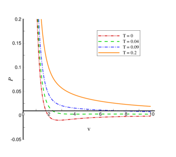
(a) $\alpha=0$, $\beta=2$, $q=b=1$ and $k=1$

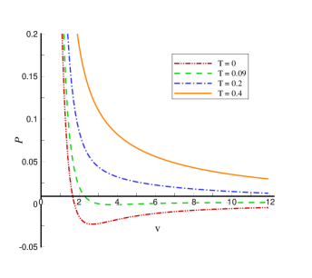
(b) $\alpha=0.5$, $\beta=2$, $q=b=1$ and $k=1$

Figure 1: $P-v$ diagram of END black holes.

III.4 Gibbs free energy

Another important approach to determine the critical behavior of a system refers to study its thermodynamic potential. In the canonical ensemble and extended phase space, thermodynamic potential closely associates with the Gibbs free energy $G=M-TS$. It is a matter of calculation to show that

$$G_{\rm END} = \frac{\omega(\alpha^{2}+1)b^{\gamma}}{8\pi}\Bigg{\{}\frac{k~{}r_{+}}{2(\alpha^{2}+1)b^{\gamma}}+\frac{(\Lambda+2\beta^{2})(\alpha^{2}-1)b^{\gamma}}{2(\alpha^{2}-3)r_{+}^{2\gamma-3}}+2q\beta\left(\frac{q}{\beta b^{\gamma}}\right)^{\frac{\gamma-1}{\gamma-2}}L_{W}(\eta_{+})^{-\frac{2\gamma-3}{2\gamma-4}}$$ (47)

$$\times\left[\frac{L_{W}(\eta_{+})^{2}}{\alpha^{2}+5}\digamma\left(\left[\frac{\alpha^{2}+5}{4}\right],\left[\frac{\alpha^{2}+9}{4}\right],\frac{\alpha^{2}-1}{4}L_{W}(\eta_{+})\right)-\frac{1}{\alpha^{2}-3}\digamma\left(\left[\frac{\alpha^{2}-3}{4}\right],\left[\frac{\alpha^{2}+1}{4}\right],\frac{\alpha^{2}-1}{4}L_{W}(\eta_{+})\right)\right]$$

$$-q\beta r_{+}^{1-\gamma}\left[\frac{1}{\sqrt{L_{W}(\eta_{+})}}-\sqrt{L_{W}(\eta_{+})}\right]\Bigg{\}}.$$

Expanding for large $\beta$ in the absence of dilaton field ($\alpha=0$), we arrive at

$$G_{\rm END}\Big{|}_{\beta\rightarrow\infty}=\frac{k~{}r_{+}}{4}-\frac{2\pi r_{+}^{3}P}{3}+\frac{3q^{2}}{4r_{+}}-\frac{7q^{4}}{80r_{+}^{5}\beta^{2}}+O\left(\frac{1}{\beta^{2}}\right).$$ (48)

This is nothing but the Gibbs free energy of RN-AdS black holes with a nonlinear leading order correction term MannRN . In order to study the Gibss free energy, we plot Fig. 3(a). One can see swallow-tail behavior in this figure which indicates a phase transition under a critical value of temperature.

III.5 Critical exponents

Here we would like to study critical exponents for END case. For this purpose, we first calculate the specific heat as

$$C_{V}=T\left(\frac{\partial S}{\partial T}\right)\Big{|}_{V}.$$ (49)

We also redefine Eq. (23) as

$$S=S(V,T)=\frac{b^{\gamma}\omega}{4}\left[\frac{(\alpha^{2}+3)V}{(\alpha^{2}+1)b^{\gamma}}\right]^{{(\gamma-2)}/{(\gamma-3)}}.$$ (50)

It is clear that entropy does not depend on the temperature in this relation, so $C_{V}=0$. This indicates that relative critical exponent will be zero

$$C_{V}\propto\left(\frac{T}{T_{c}}-1\right)^{\alpha^{\prime}}\Rightarrow\alpha^{\prime}=0.$$ (51)

In order to find other critical exponent we consider the following definition

$$\tau=\frac{T}{T_{c}}\qquad\qquad p=\frac{P}{P_{c}}\qquad\qquad\nu=\frac{V}{V_{c}}.$$ (52)

Thus, we find

$$p\mid_{\rm END} = \frac{1}{\rho_{c}}\frac{\tau}{\nu}-\frac{k(\alpha^{2}+3)}{8\pi P_{c}(\alpha^{2}-3)(\alpha^{2}-1)}\frac{(v_{c}\nu\Gamma)^{\gamma-2}}{b^{\gamma}}-\frac{\beta^{2}(\alpha^{2}+3)}{4\pi P_{c}(\alpha^{2}-3)}\left(\frac{b}{v_{c}\nu\Gamma}\right)^{\gamma}$$ (53)

$$-\frac{q\beta(\alpha^{2}+3)}{4\pi P_{c}(\alpha^{2}-3)(v_{c}\nu\Gamma)^{2}}\bigg{(}\sqrt{L_{W}(\eta^{\prime\prime})}-\frac{1}{\sqrt{L_{W}(\eta^{\prime\prime})}}\bigg{)},$$

where

$$\eta^{\prime\prime}=\left(\frac{q~{}(v_{c}\nu\Gamma)^{\gamma-2}}{\beta~{}b^{\gamma}}\right)^{2}.$$ (54)

Expanding for $\beta\rightarrow\infty$, yields

$$p=\frac{1}{\rho_{c}}\frac{\tau}{\nu}+\frac{1}{4\pi P_{c}}\Bigg{\{}\frac{k(\alpha^{2}+1)\Gamma b^{-\gamma}}{(\alpha^{2}-1)(\nu\Gamma v_{c})^{2-\gamma}}-\frac{q^{2}(\alpha^{2}+3)(\nu\Gamma v_{c})^{2\gamma-4}}{2(\alpha^{2}-3)b^{\gamma}(\nu\Gamma)^{\gamma}}\Bigg{\}}.$$ (55)

Since we would like to find critical exponent, we should consider the close neighborhood of critical point, so we expand Eq. (53) near the critical point. Considering $\tau=t+1$ and $\nu=(\omega+1)^{1/\epsilon}$ where $\epsilon=(\alpha^{2}+3)/(\alpha^{2}+1)$, and taking into account relation (53), we get

$$p=1+At-Bt\omega-C\omega^{3}+O(t\omega^{2},\omega^{4}),$$ (56)

where

$$A=\frac{1}{\rho_{c}}\qquad B=\frac{1}{\epsilon\rho_{c}}\qquad C=\frac{2(\alpha^{2}+2)}{3(\alpha^{2}+1)^{2}\epsilon^{3}}-\frac{(\alpha^{2}+7)q^{2\gamma-2}}{3(\alpha^{2}+3)^{3}\beta^{2}b^{2\gamma}}\left(\frac{k}{(\alpha^{2}+3)(\alpha^{2}+2)}\right)^{2-\gamma}.$$ (57)

According to the Maxwell’s equal area law MannRN , we get

$$p=1+At-Bt\omega_{l}-C\omega_{l}^{3}=1+At-Bt\omega_{s}-C\omega_{s}^{3}$$

$$0=-P_{c}\int\limits_{\omega_{l}}^{\omega_{s}}\omega(Bt+3C\omega^{2})d\omega,$$ (58)

where we $\omega_{l}$ and $\omega_{s}$ refers to volume of large and small black holes. The only non-trivial solution of Eq. (III.5) is

$$\omega_{l}=\omega_{s}=2\sqrt{-\frac{Bt}{C}}.$$ (59)

The behavior of the order parameter near the critical point can be found as

$$\Xi=V_{c}(\omega_{l}-\omega_{s})=2V_{c}\omega_{l}=2\sqrt{-\frac{B}{C}}t^{1/2}.$$ (60)

Therefore, the critical exponent associated with the order parameter should be $\beta^{\prime}=\frac{1}{2}$ which coincides with that in Van der Waals gas. Isothermal compressibility near the critical point can be obtained as

$$\kappa_{T}=-\frac{1}{V}\frac{\partial V}{\partial P}\Bigg{|}_{T}\propto-\frac{V_{c}}{BP_{c}}\frac{1}{t}.$$ (61)

Since $\kappa_{T}\propto t^{-\gamma^{\prime}}$, we have $\gamma^{\prime}=1$ and as we expect near the critical point it should diverge. The last critical exponent is $\delta^{\prime}$ which describes the relation between order parameter and ordering field in the critical point, so we should set $t=0$ in Eq. (56). We find

$$p-1=-C\omega^{3}\qquad\Longrightarrow\qquad\delta^{\prime}=3.$$ (62)

It is important to note that all critical exponents in this theory coincide with those of Van der Waals gas system.

IV Critical behavior of LND black holes

Now, we can repeat all above steps for LND electrodynamics and consider the effect of this type of nonlinear electrodynamics on the critical behaviour of the solutions. At first, we introduce metric function and vector potential for this type of black holes sara

$$A_{t}^{\rm LND}=\frac{q}{r}~{}{}_{3}\digamma_{2}\left(\left[\frac{1}{2},1,\frac{\alpha^{2}+1}{4}\right],\left[2,\frac{\alpha^{2}+5}{4}\right],-\eta\right)$$ (63)

$$f(r)_{\rm LND} = -k\frac{{\alpha}^{2}+1}{{\alpha}^{2}-1}{b}^{-\gamma}{r}^{\gamma}-\frac{m}{r^{1-\gamma}}+\frac{(\Lambda-4\beta^{2})\left({\alpha}^{2}+1\right)^{2}{b}^{\gamma}}{\alpha^{2}-3}r^{2-\gamma}+\frac{8\beta^{2}{(\alpha^{2}+1)^{2}}}{(\alpha^{2}-3)^{2}}b^{\gamma}r^{2-\gamma}$$ (64)

$$\times\Bigg{\{}1-{}_{2}\digamma_{1}\left(\left[-\frac{1}{2},\frac{\alpha^{2}-3}{4}\right],\left[\frac{\alpha^{2}+1}{4}\right],-\eta\right)+\frac{\alpha^{2}-3}{2}\left(\sqrt{1+\eta}-\ln\left(\frac{\eta}{2}\right)+\ln\left(-1+\sqrt{1+\eta}\right)\right)\Bigg{\}}$$

where ${}_{2}\digamma_{1}$ and ${}_{3}\digamma_{2}$ is the hypergeometric functions. In order to study thermodynamics quantities, we first find temperature as

$$T_{+}^{\rm LND}=-2k\frac{r_{+}^{\gamma-1}b^{-\gamma}}{4\pi}-\frac{m(\alpha^{2}-3)}{4\pi(\alpha^{2}+1)}r_{+}^{\gamma-2}+\frac{8\beta^{2}(\alpha^{2}+1)}{4\pi(\alpha^{2}-3)}b^{\gamma}r^{1-\gamma}\left(1-\frac{1}{\sqrt{1+\eta_{+}}}\right)+\frac{8q^{2}}{4\pi(\alpha^{2}-3)}b^{-\gamma}r_{+}^{\gamma-3}$$

$$\qquad\qquad\times\Bigg{\{}2\times{}_{2}\digamma_{1}\left(\left[\frac{1}{2},\frac{\alpha^{2}+1}{4}\right],\left[\frac{\alpha^{2}+5}{4}\right],-\eta_{+}\right)-\frac{\alpha^{2}+1}{\sqrt{1+\eta_{+}}}\Bigg{\}}.$$ (65)

The entropy expression is the same as END case, because it does not depend on electrodynamics and still obeys the area law. Considering the definition of electric potential, one may obtain $U$ as

$$U_{\rm LND}=\frac{q}{r_{+}}~{}{}_{3}\digamma_{2}\left(\left[\frac{1}{2},1,\frac{\alpha^{2}+1}{4}\right],\left[2,\frac{\alpha^{2}+5}{4}\right],-\eta_{+}\right).$$ (66)

In order to verify the first law of thermodynamics, we should calculate conjugate of nonlinear parameter for LND topological black hole. We obtain

$$B_{\rm LND} = \frac{(\alpha^{2}+1)\beta b^{2\gamma}}{\pi(\alpha^{2}-3)r_{+}^{2\gamma-3}}\Bigg{\{}\sqrt{1+\eta_{+}}-\ln\left(\frac{\eta_{+}}{2}\right)+\ln(\sqrt{1+\eta_{+}}-1)-\frac{\eta_{+}}{2\sqrt{1+\eta_{+}}}\left(1+\frac{1}{\sqrt{1+\eta_{+}}-1}\right)+\frac{2}{\alpha^{2}-3}$$ (67)

$$\times\left(1-{}_{2}\digamma_{1}\left(\left[-\frac{1}{2},\frac{\alpha^{2}-3}{4}\right],\left[\frac{\alpha^{2}+1}{4}\right],-\eta_{+}\right)\right)+\frac{\eta_{+}}{(\alpha^{2}+1)}~{}{}_{2}\digamma_{1}\left(\left[\frac{1}{2},\frac{\alpha^{2}+1}{4}\right],\left[\frac{\alpha^{2}+5}{4}\right],-\eta_{+}\right)\Bigg{\}},$$

which its asymptotic behavior for $\beta\rightarrow\infty$ and $\alpha=0,1$ can be obtained as

$$B_{\rm LND}\Big{|}_{\beta\rightarrow\infty,\alpha=0}=\frac{q^{4}\omega}{160\pi r^{5}\beta^{3}}-\frac{q^{6}\omega}{432\pi r^{9}\beta^{5}}+O\left(\frac{1}{\beta^{7}}\right)$$

$$B_{\rm LND}\Big{|}_{\beta\rightarrow\infty,\alpha=1}=\frac{q^{4}\omega}{96\pi r^{3}b^{2}\beta^{3}}-\frac{q^{6}\omega}{240\pi r^{5}b^{4}\beta^{5}}+O\left(\frac{1}{\beta^{7}}\right).$$ (68)

It is clear that this relation is similar to those given in Eq. (33). Definition of black holes thermodynamic volume is related to the entropy and since the entropy expression does not depend on the type of electrodynamics, so thermodynamics volume is the same as given in Eq. (25). Also, as we mentioned before, the pressure is related to the cosmological constant, so for LND black holes, one can find that the pressure is exactly the same as given in Eq. (34). Finally, it is a matter of calculation to check that all conserved and thermodynamic quantities of LND black holes satisfy the first law of black thermodynamics (27) as well as Smarr relation (35).

IV.1 Equation of state

This section is devoted to study the critical behavior of black hole in the presence of LND electrodynamics. In this regard, we obtain equation of state at first

$$P_{\rm LND} = \frac{T}{v}+\frac{1}{4\pi v}\frac{k~{}(\alpha^{2}+1)}{b^{\gamma}(\alpha^{2}-1)}(\Gamma v)^{\gamma-1}-\frac{4}{\pi v}\frac{q^{2}~{}(\Gamma v)^{\gamma-3}}{b^{\gamma}(\alpha^{2}-3)}{}_{2}\digamma_{1}\Bigg{(}\left[\frac{1}{2},\frac{\alpha^{2}+1}{4}\right],\left[\frac{\alpha^{2}+5}{4}\right],-\eta^{\prime}\Bigg{)}+\frac{1}{\pi v}\frac{\beta^{2}b^{\gamma}(\alpha^{2}+1)}{(\Gamma v)^{\gamma-1}}$$ (69)

$$\times\Bigg{\{}-\frac{2}{\alpha^{2}-3}{}_{2}\digamma_{1}\Bigg{(}\left[-\frac{1}{2},\frac{\alpha^{2}-3}{4}\right],\left[\frac{\alpha^{2}+1}{4}\right],-\eta^{\prime}\Bigg{)}+\ln(\sqrt{1+\eta^{\prime}}-1)-\ln(\eta^{\prime})+\ln(2)-1\Bigg{\}}$$

$$+\frac{1}{\pi v}\frac{(\alpha^{4}-1)b^{\gamma}}{(\alpha^{2}-3)\sqrt{1+\eta^{\prime}}}\Big{[}q^{2}b^{-2\gamma}(\Gamma v)^{2\gamma-4}+\beta^{2}\Big{]}(\Gamma v)^{1-\gamma}.$$

It is a general belief that one can predict a Van der Walls like behavior for a thermodynamic system by studying its $P-v$ diagrams. According to Fig. 2 we can observe that for specific values of parameters, phase transition exist below a critical temperature. It occurs for both large (Fig.2(a)) and small (Fig. 2(b)) value of nonlinear parameter in the presence of dilaton field.

One may find the properties of critical point by using Eq. (69). However, due to the complexity of this equation, it is not easy to investigate the critical point for arbitrary nonlinear parameter. Therefore, we consider the large $\beta$ limit of Eq. (69),

$$P_{\rm LND}\Big{|}_{\beta\rightarrow\infty}=\frac{T}{v}+\frac{(\alpha^{2}+1)}{4\pi vb^{\gamma}}\Bigg{\{}-\frac{k}{(\alpha^{2}-1)}(v\Gamma)^{\gamma-1}+q^{2}(v\Gamma)^{\gamma-3}-\frac{q^{4}}{8b^{2\gamma}\beta^{2}}(v\Gamma)^{3\gamma-7}\Bigg{\}}.$$ (70)

In the absence of dilaton field ($\alpha=0$), the equation of state of RN-AdS black holes in an extended phase space MannRN is recovered with a leading order nonlinear correction term

$$P_{\rm LND}\Big{|}_{\beta\rightarrow\infty}=\frac{T}{v}-\frac{k}{2\pi v^{2}}+\frac{2q^{2}}{\pi v^{4}}-\frac{4q^{4}}{\pi v^{8}\beta^{2}}.$$ (71)

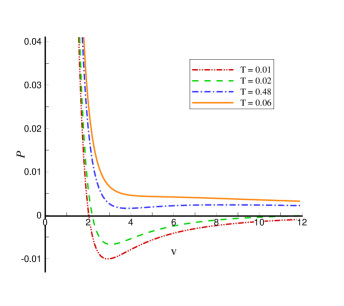
(a) $\alpha=0.3$, $\beta=2$, $q=b=1$ and $k=1$

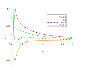
(b) $\alpha=\beta=0.2$, $q=b=1$ and $k=1$

Figure 2: $P-v$ diagram of LND black holes

Therefore, for large $\beta$ limit, the critical point is obtained as

$$v_{c}=\frac{\Pi}{\Gamma}-\frac{5q^{4}(\alpha^{2}+4)(\alpha^{2}+7)}{16\Gamma k\beta^{2}b^{2\gamma}}\Pi^{2\gamma-5}+O\left(\frac{1}{\beta^{4}}\right),$$

$$P_{c}=\frac{q^{2}(\alpha^{2}+3)^{2}}{8\pi(\alpha^{2}-3)b^{\gamma}}\Pi^{\gamma-4}+\frac{5q^{4}(\alpha^{2}+7)}{32\pi\beta^{2}b^{3\gamma}}\Gamma\Pi^{3\gamma-8}+O\left(\frac{1}{\beta^{4}}\right),$$

$$T_{c}=-\frac{k(\alpha^{2}+1)}{\pi(\alpha^{2}-1)(\alpha^{2}+3)b^{\gamma}}\Pi^{\gamma-1}+\frac{5q^{4}(\alpha^{2}+4)}{16\pi\beta^{2}b^{3\gamma}}\Pi^{3\gamma-7}+O\left(\frac{1}{\beta^{4}}\right),$$

$$\rho_{c}=-\frac{(\alpha^{2}+3)(\alpha^{2}-1)}{4(\alpha^{2}+2)}\Bigg{\{}1-\frac{5q^{2}}{4(\alpha^{2}+2)\beta^{2}b^{2\gamma}}\Pi^{2\gamma-4}\Bigg{\}}+O\left(\frac{1}{\beta^{4}}\right).$$ (72)

It is important to note that all above relations reduce to those of RN-AdS black holes in an extended phase space MannRN provided $\alpha=0$ and $\beta\rightarrow\infty$. Comparing the results obtained here with relation (III.3), one can find that the critical point in the large $\beta$ expansion for both electrodynamics are similar and the same as those of BID given in Dayyani1 . This is an expected result since in the large $\beta$ limit, the Lagrangian of all of these theories have similar expansion, namely

$$L_{\rm BID}=L_{\rm END}=-F^{2}e^{-2\alpha\phi(r)}+\frac{F^{4}}{8\beta^{2}}e^{-6\alpha\phi(r)}+O\left(\frac{1}{\beta^{4}}\right),$$

$$\qquad~{}~{}~{}~{}~{}L_{\rm END}=-F^{2}e^{-2\alpha\phi(r)}+\frac{F^{4}}{16\beta^{2}}e^{-6\alpha\phi(r)}+O\left(\frac{1}{\beta^{4}}\right).$$ (73)

Thus for large $\beta$ the equation of state and the critical point properties of BID, END and LND electrodynamics are the same.

IV.2 Gibbs free energy

Next, we study Gibbs free energy for LND black holes to characterize phase transition in the system. It is a matter of calculation to show that the Gibbs free energy of LND black holes is given by

$$G_{\rm LND} = \frac{k~{}r_{+}\omega}{16\pi}+\frac{(\alpha^{2}+1)r^{3-2\gamma}\omega}{4\pi(\alpha^{2}-3)}\Bigg{\{}\frac{2\pi P(\alpha^{2}-3)(\alpha^{2}-1)(b~{}r_{+})^{\gamma}}{(\alpha^{2}+3)}+\frac{2q^{2}r_{+}^{2\gamma-4}}{\sqrt{1+\eta_{+}}}$$ (74)

$$+b^{2\gamma}\beta^{2}\Bigg{[}(\alpha^{2}-1)\ln\left(\frac{2\sqrt{1+\eta_{+}}}{\eta_{+}}-\frac{2}{\eta_{+}}\right)+\frac{(\alpha^{2}-1)\eta_{+}+\alpha^{2}+1}{\sqrt{1+\eta_{+}}}-\frac{\alpha^{4}-4\alpha^{2}-1}{(\alpha^{2}-3)}\Bigg{]}-\frac{2(\alpha^{2}-1)\beta^{2}b^{2\gamma}}{(\alpha^{2}-3)}$$

$$\times{}_{2}\digamma_{1}\Bigg{(}\left[-\frac{1}{2},\frac{(\alpha^{2}-3)}{4}\right],\left[\frac{(\alpha^{2}+1)}{4}\right],-\eta_{+}\Bigg{)}-\frac{4q^{2}r_{+}^{2\gamma-4}}{(\alpha^{2}+1)}{}_{2}\digamma_{1}\Bigg{(}\left[\frac{1}{2},\frac{(\alpha^{2}+1)}{4}\right],\left[\frac{(\alpha^{2}+5)}{4}\right],-\eta_{+}\Bigg{)}\Bigg{\}}.$$

Note that if we expand this relation for large nonlinear parameter $\beta$, we restore the result of Eq. (48). We have plotted the behavior of Gibbs free energy in term of temperature in Fig. 3(b). one can observes swallow-tail behavior in this figure when pressure is smaller that its critical value. This implies that the system experiments a phase transition.

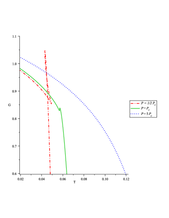
(a) END black holes

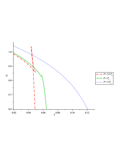
(b) LND black holes

Figure 3: Gibbs free energy versus $T$ for $\beta=q=b=k=1$ and $\alpha=0.3$.

IV.3 Critical exponents

Next, we are going to obtain the critical exponent of LND black holes. As we mentioned before, the entropy is equal in both theories, so $C_{v}$ is equal too, and $\alpha^{\prime}=0$ like BID and END theories. In order to calculate other critical exponent we should follow the approach given in subsection III.5. To this end, we compute the equation of state near the critical point for LND theories

$$p=1+At-Bt\omega-C^{\prime}\omega^{3}+O(t\omega^{2},\omega^{4}),$$ (75)

where

$$C^{\prime} = \frac{2(\alpha^{2}+2)}{3(\alpha^{2}+3)^{2}\epsilon}-\frac{5(\alpha^{2}+7)q^{2\gamma-2}}{6(\alpha^{2}+3)^{3}\beta^{2}b^{2\gamma}}\left(\frac{k}{(\alpha^{2}+3)(\alpha^{2}+2)}\right)^{2-\gamma}.$$ (76)

It is clear that the form of the above relation is similar to relation (56), so as one expects all remind critical exponent will be the same as in the case of END theory.

V Effects of nonlinear gauge field

Although, we have calculated the critical quantities in the limit of large $\beta$ where the nonlinearity of the theory is small. However, it is clear from the $P-v$ and Gibbs diagrams that there is a similar phase transition in the limit of small $\beta$ where the nonlinearity of the theory is large. In the limit of small $\beta$ it is nearly impossible to calculate analytically the critical quantities. Also, in the presence of the dilaton field, it will be very difficult to calculate them even numerically. For some numeric calculations (in the absence of dilaton field) one may see Hendi1 .

A close look at the critical temperature in both END and LND given in Eqs. (III.3) and (IV.1), show that the presence of the nonlinear field makes the critical temperature larger and it will increase with decreasing $\beta$. One may observe that the increasing in $T_{c}$ and $p_{c}$ in LND is stronger than END. In Fig. 4 we have plotted critical quantities $T_{c}$ and $p_{c}$ of LND, END and Maxwell-dilaton (MD) theory in terms of the nonlinear parameter $\beta$ and show that they will go to a same value in the large limit of $\beta$ where the effects of nonlinearity disappears. Clearly, the linear MD theory is independent of the nonlinear parameter $\beta$, as can be seen from Fig. 4. It is notable to mention that critical quantities in LND are the same as those in END for large $\beta$. However, for small $\beta$ (nonlinear regime), their behaviour is quit different. The behavior of the critical temperature in term of $\alpha$ is shown in Fig 5, for $0\leq\alpha<1$. From these figures, one can see that the behaviour of the diagrams differ as the nonlinear parameter $\beta$ decreases. This implies that in a very strong nonlinear regime, the nonlinearity nature of the theory plays a crucial role. When $\alpha\rightarrow 1$, the critical temperatures in different type of electrodynamic fields toward each others but it is completely unlike the critical pressure. As one see in Fig. 6, for $\alpha\rightarrow 1$, the critical pressures become more different.

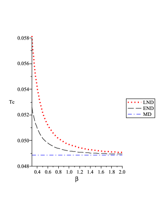
(a) $T_{c}$ versus $\beta$

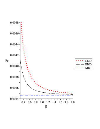
(b) $P_{c}$ versus $\beta$

Figure 4: Critical quantities of dilaton black holes. Here we have set $q=b=k=1$ and $\alpha=0.2$.

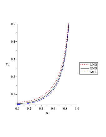
(a) $\beta=0.25$

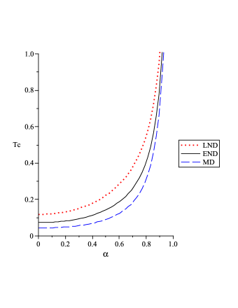
(b) $\beta=0.1$

Figure 5: $T_{c}$ versus $\alpha$ of dilaton black holes with different electrodynamics. Here we have taken $q=b=k=1$.

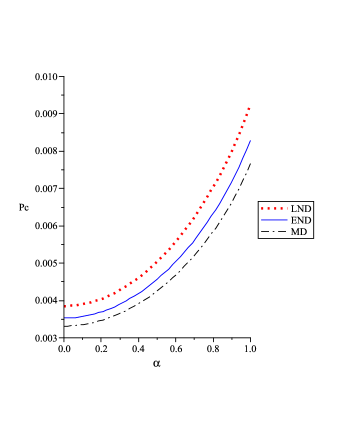
(a) $\beta=0.5$

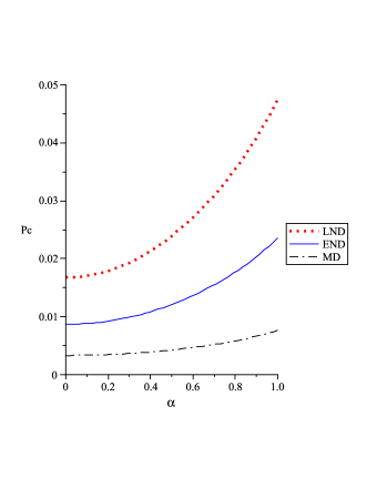
(b) $\beta=0.1$

Figure 6: $P_{c}$ versus $\alpha$ of black holes in different electrodynamics with $q=b=k=1$

As we already pointed out, although it is hard to calculate the critical quantities analytically for arbitrary $\beta$, however it is quite possible to plot the related diagrams for different $\beta$. We study Gibbs free energy and $P$-$v$ behaviour in Figs. 7 and 8, to see the the difference between the nonlinear theories we have considered. It is clear from these diagrams that the behavior of END, LND and BID black holes is very similar when $T$ or $\beta$ are large enough. As one expects, in the same $T$, the difference between diagrams increase as $\beta$ decreases (see Fig. 9).

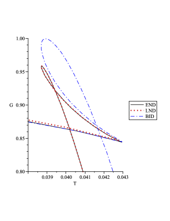
(a) $\beta=1$

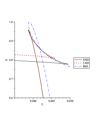
(b) $\beta=0.25$

Figure 7: Gibbs free energy versus $T$ of dilaton black holes for $q=b=k=1$ and $\alpha=0.2$

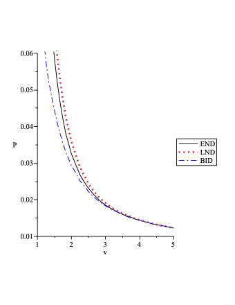
(a) $\beta=0.5$ and $T=0.1$

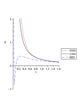
(b) $\beta=0.25$ and $T=0.3$

Figure 8: P-v diagram of dilaton black holes with different electrodynamics. Here we have taken $\alpha=0.3$ and $q=b=k=1$.

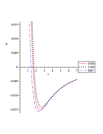
(a) $\beta=0.7$

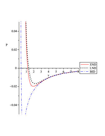
(b) $\beta=0.4$

Figure 9: $P-v$ diagram of dilaton black holes in the same temperature $T=0.001$ and different $\beta$. Here we have fixed $\alpha=0.3$ and $q=b=k=1$.

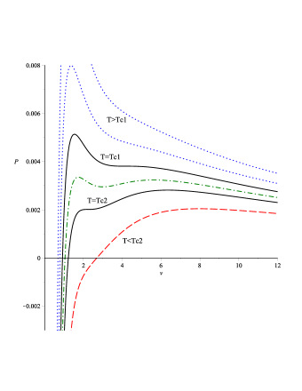
(a) $\alpha=0$

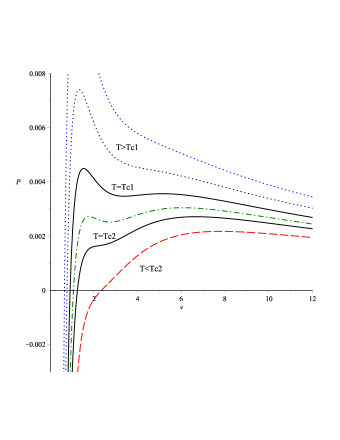
(b) $\alpha=0.1$

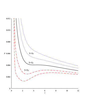
(c) $\alpha=0.25$

Figure 10: $P-v$ diagram for BID black holes. Here we have fixed $\beta=0.45$, $q=b=1$ and $k=1$.

It was extensively argued in MannBI that in the absence of dilaton field, black hole with BI nonlinear electrodynamics may have two, one or zero critical points which depends on the strength of nonlinear and charge parameters. For BID black holes, only for small values of dilaton-electromagnetic coupling $\alpha$ one may see second critical point. Interestingly enough, as dilaton parameter $\alpha$ increases, the second critical point disappears. As an example, we compare $P-v$ diagrams of BID black holes for three values of dilaton coupling $\alpha$ in Fig. 10. It is clear from these diagrams that in the absence of dilaton field (Fig. 10(a)) or for weak dilaton field (Fig. 10(b)), there are two critical points but when dilaton field increases (Fig. 10(c)) the second critical point vanish and we have only one critical point. In the other types of nonlinear electrodynamics such as Logarithmic, Exponential or Power-law Maxwell fields, the second critical point is never seen neither in the absence nor in the presence of dilaton field. Also it is worthwhile to mention that for very small value of nonlinear parameter $\beta$ there is not any critical point in all types of above electrodynamics.

VI Zeroth order phase transition

Let us emphasize that the observed phase transition in the previous sections which were similar to the Van der Walls phase transition is called the first order phase transition in the literature. It occurs where Gibbs free energy is continuous, but its first derivative respect to the temperature and pressure is discontinuous. Now we want to mention that another interesting type of phase transition happens in the certain range of the metric parameters. This discontinuity in Gibbs free energy known as zeroth order phase transition which is observed in superfluidity and superconductivity 20MrDeh . It is important to note that, due to this transition, the response functions of black holes thermodynamics diverge e.g. isothermal compressibility. Recently, zeroth order phase transition was observed in the context of Einstein-Maxwell-dilaton black holes MrDeh . It was confirmed that the presence of dilaton field plays a crucial role for such a phase transition MrDeh . Indeed, there is a direct relation exists between the zeroth-order portion of the transition curve and dilaton parameter $\alpha$ MrDeh . In other words, we have no zeroth order phase transition for Einstein-Maxwell (Reissner-Nordstrum) black holes. Moreover, for nonlinear BI electrodynamics, it was shown that a zeroth order phase transition may occur even in the absence of dilaton field R.Mann , which means that the nonlinearity of the gauge field can also cause a zeroth order phase transition in black holes thermodynamics.

Here we would like to explore the possibility to have such a zeroth order phase transition in END and LND black holes, where both nonlinearity and dilaton field are taken into account. In order to see the finite jump in Gibbs free energy, we plot the diagrams of Gibbs free energy respect to the pressure in Figs. 11, 12 and 13 for different values of the metric parameters.

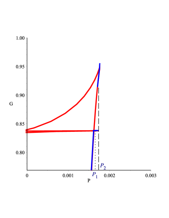
Figure 11: Gibbs free energy for BID black holes versus pressure for $T=0.732T_{c}$. Here we have fixed $q=b=1$, $\alpha=0.025$, $\beta=0.45$.

(a) BID black hole

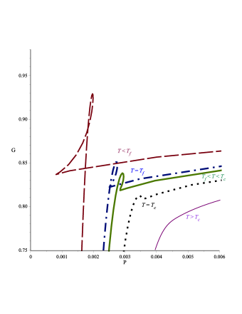
(b) END black hole

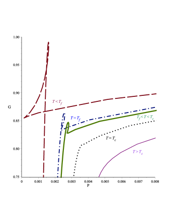
(c) LND black hole

Figure 12: Gibbs free energy versus pressure for $\alpha=0.2$, $\beta=0.45$ and $q=k=b=1$.

For completeness, we also investigate the phase transition of BID solutions presented in Dayyani1 . An interesting case in the BID theory is plotted in Fig. 11. From this figure, we see that for a certain values of pressure and especial range of dilaton field parameter, both zeroth and first order phase transitions may be observed in one diagram. Based on this figure, by increasing the pressure until $P_{1}$ a first order transition occurs. For $P>P_{1}$, Gibbs free energy has two values and as one can see, the acceptable values of energy are shown in the blue curve since it includes smaller values of energy. At point $P_{2}$, one can see a discontinuity in Gibbs free energy which demonstrates a zeroth order phase transition.

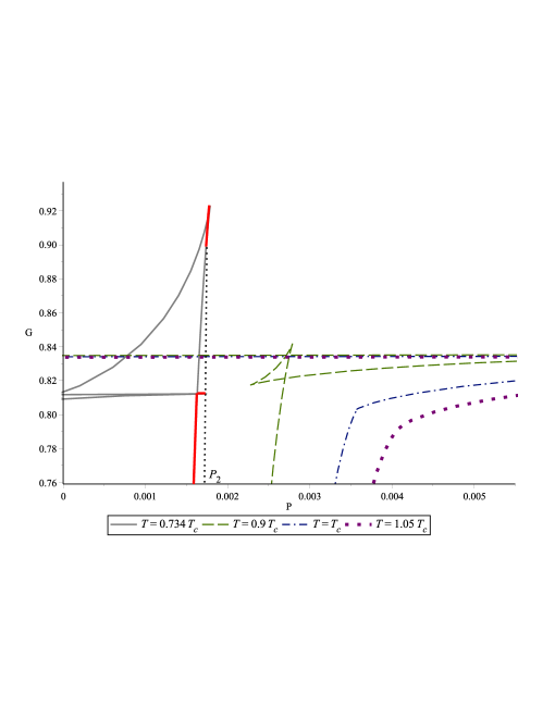
(a) BID black hole

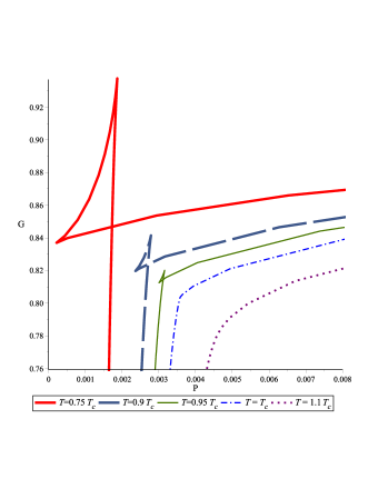
(b) END black hole

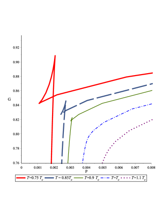
(c) LND black hole

Figure 13: Gibbs free energy versus pressure for $\alpha=0$, $\beta=0.45$ and $q=k=b=1$.

Also, Fig. 12 shows different critical behaviors of dilatonic black holes in the presence of three nonlinear electrodynamics respect to the changes in the temperature values when other metric parameters are fixed. In the case of $T>T_{c}$, we have no phase transition. When $T=T_{c}$, the system experiences a second order phase transition as we have discussed before. As temperature decreases to the $T_{\rm f}<T<T_{c}$ a zeroth order phase transition is observed. Finally, at $T=T_{\rm f}$ the first order phase transition occurs. It is worth mentioning that this behavior is repeated in the Gibbs free energy of all three types of black holes in the presence of nonlinear electrodynamics and non-zero values of dilaton field.

It is important to note that by looking at Fig. 13, one may wonder that, for fixed values of the parameters, and in the absence of dilaton field ($\alpha=0$), we do not observe zeroth order phase transition in END and LND theories. This is in contrast to the BID theory where a zeroth order phase transition is occurred in the small range of nonlinear parameters $\beta$ even in the absence of dilaton field (see Fig. 13(a)). In this figure, the red portion curve shows this behavior as we explained in close-up Fig. 11. It is one of the main difference between these three nonlinear electrodynamics, which implies that their behavior in case of small values of $\beta$ completely differ. This indicate that, while the nonlinearity can lead to zeroth order phase transition in BI theory, it is not the case for EN and LN theories. In other words, the presence of the dilaton field plays a crucial role for occurring zeroth order phase transition in the context of END and LND electrodynamics.

VII Closing remarks

In this paper, we have studied critical behavior and phase transition of Exponential and Logarithmic nonlinear electrodynamics in the presence of dilaton field, which we labeled them as END and LND, respectively. We extended the phase space by considering the cosmological constant and nonlinear parameter as thermodynamic variables. We introduced common conditions to find solution in both theories, such as potential, metric and etc. We have investigated these tow nonlinear theories, separately. As the expansion of END Lagrangian for large nonlinear parameter, $\beta$, and BID is exactly the same, it is expected that their critical behavior be the same, in the limit of $\beta\rightarrow\infty$. We continued our calculation by obtaining equation of state of END black holes. We observed that $P-v$ diagrams of this theory are similar to those of Wan der Waals gas. By applying the approach of Wan der Waals gas to find out the critical point, we concluded that this point is exactly the same as in BID black holes. Besides, the Gibbs free energy diagram confirmed the existence of phase transition and finally critical exponents were obtained which are exactly the same as the mean field theory.

We also investigated the critical behaviour of LND black holes. Again, for $\beta\rightarrow\infty$, the series expansion of LND Lagrangian is similar to END and BID cases, so one expects that critical behavior of this theory to be similar to BID and END theories in this limit. Our calculations confirmed that the critical behavior of LND theory is exactly the same as those of a Wan der Waals gas system.

It is important to note that although the critical behaviour of END and LND electrodynamics, in the limit of large nonlinear parameter $\beta$, is similar to BID black holes explored in Ref. Dayyani1 , however, for small value of $\beta$, the situation quite differs and the behaviour of these three type of nonlinear electrodynamics are completely different. For example, it was argued in MannBI that BI black holes may have two, one or zero critical points, however, this behaviour is not seen for Logarithmic and Exponential, namely the second critical point is never seen in the absence/presence of dilaton field.

We also investigated the phase transition of END and LND black holes. In addition to the usual critical (second-order) as well as the first-order phase transitions in END and LND black holes, we observed that a finite jump in Gibbs free energy is generated by dilaton-electromagnetic coupling constant, $\alpha$, for a certain range of pressure. This novel behavior indicates a small/large black hole zeroth-order phase transition in which the response functions of black holes thermodynamics diverge. It is worthy to note that for temperature in the range $T_{\rm f}<T<T_{c}$, a discontinuity occurs in the Gibbs free energy diagram which leads to zeroth order phase transition. We find out that in the absence of dilaton field, we do not observe zeroth order phase transition in END and LND theories. This is in contrast to the BI theory where a zeroth order phase transition is occurred in the small range of nonlinear parameters $\beta$ even in the absence of dilaton field. We conclude that, while in BI black holes, the nonlinearity can lead to zeroth order phase transition, it is not the case for EN and LN black holes. In other words, the presence of dilaton field plays a crucial role for occurring zeroth order phase transition in the context of EN and LN electrodynamics.

Finally, we would like to mention that the jump in the Gibbs free energy is observed for three types of dilatonic nonlinear electrodynamics, namely BID, END and LND. However, in the absence of dilaton field, a zeroth order phase transition occurs only for BI black holes, which means that the nonlinearity is responsible for this phase transition. However, for LND and END black holes, it seems the dilaton field is responsible for this type of zeroth order phase transition. Albeit, for BID theory, both dilaton field as well as nonlinear electrodynamics can lead to zeroth order phase transition. This behaviour and the physical reasons behind it, need further investigations in the future studies.

References

• (1) J.D. Bekenstein, Phys. Rev. D 7, 2333 (1973); J.D. Bekenstein, Phys. Rev. D 9, 3292 (1974).
• (2) S.W. Hawking, Commun. Math. Phys. 43, 199 (1975); S.W. Hawking, Phys. Rev. D 13, 191 (1976).
• (3) S. Hawking and D. N. Page, Commun. Math. Phys. 87, 577 (1983).
• (4) B. P. Dolan, Class. Quant. Grav. 28, 235017 (2011).
• (5) D. Kastor, S. Ray, and J. Traschen, Class. Quant. Grav. 26, 195011 (2009).
• (6) B. Dolan, Class. Quant. Grav. 28, 125020 (2011).
• (7) B. P. Dolan, Phys. Rev. D 84, 127503 (2011).
• (8) M. Cvetic, G. W. Gibbons, D. Kubiznak, and C. N. Pope, Phys. Rev. D 84, 024037 (2011).
• (9) M. Urana, A. Tomimatsu, and H. Saida, Class. Quant. Grav. 26, 105010 (2009).
• (10) D. Kubiznak and R. B. Maan, J. High Energy Physics, 07, 033 (2012).
• (11) Sh. Gunasekaran, D. Kubiznak and R. B. Mann, JHEP, 11, 110 (2012).
• (12) S. H. Hendi, M. H. Vahidinia, Phys. Rev. D 88, 084045 (2013).
• (13) S. H. Hendi, S. Panahiyan, B. Eslam Panah, Int. J. Mod. Phys. D Vol. 25, No. 1, 1650010 (2016).
• (14) S.-W. Wei and Y.-X. Liu, Phys. Rev. D 87, 044014 (2013).
• (15) De. Zou, Y.i Liu, B. Wang, Phys.Rev. D 90, 044063 (2014).
• (16) A. Frassino, D. Kubiznak, R. Mann, and F. Simovic, JHEP 09, 080 (2014);
J. X. Mo, W. B. Liu, Eur. Phys. J. C. 74, 2836 (2014).
• (17) M. B. Jahani Poshteh, B. Mirza and Z. Sherkatghanad, Phys. Rev. D 88, 024005 (2013).
• (18) Z. Sherkatghanad, B. Mirza, Z. Mirzaeyan and S. A. Hosseini Mansoori, arXiv:1412.5028.
• (19) R. Banerjee and D. R Roychowdhury, Phys. Rev. D 85, 044040 (2012);
R. Banerjee, D. Roychowdhury, Phys. Rev. D 85, 104043 (2012).
• (20) De. Ch. Zou, Sh.-J. Zhang and B. Wang, Phys. Rev. D 89, 044002 (2014).
• (21) C. V. Johnson, Class. Quant. Grav. 31, 225005 (2014);
C. O. Lee, Phys. Let. B 09 (2014) 046.
• (22) M. Born and L. Infeld, Proc. R. Soc. A 144, 425 (1934).
• (23) H. H. Soleng, Phys. Rev. D 52, 6178 (1995).
• (24) M. Hassaine and C. Martinez, Phys. Rev. D 75, 027502 (2007).
• (25) S. H. Hendi, Phys. Lett. B 677, 123 (2009).
• (26) M. B. Green, J. H. Schwarz, and E. Witten, Superstring Theory (Cambridge University Press, Cambridge, England, 1987).
• (27) G. W. Gibbons and K. Maeda, 298(1988)741
• (28) D. Garfinkle, G. T. Horowitz and A. Strominger, Phys. Rev. D 43 (1991) 3140.
• (29) K. C. K. Chan, J. H. Horne and R. B. Mann, Nucl. Phys. B 447 (1995) 441.
• (30) G. Clement and C. Leygnac, Phys. Rev. D 70 (2004) 084018.
• (31) C. J. Gao and H. N. Zhang, Phys. Lett. B 612 (2006) 127.
• (32) R. G. Cai and K. S. Soh, Phys. Rev. D 59, 044013 (1999).
• (33) M. H Dehghani and N. Farhangkhah, Phys. Rev. D 71, 044008 (2005);
M. H. Dehghani, S. H. Hendi, A. Sheykhi and H. Rastegar Sedehi, JCAP 02 (2007) 020.
• (34) A. Sheykhi, Phys. Rev. D 76, 124025 (2007).
• (35) A. Sheykhi, N. Riazi, M. H. Mahzoon, Phys. Rev. D 74, 044025 (2006);
A. Sheykhi, Phys. Lett. B 662, 7 (2008);
A. Sheykhi, N. Riazi, Phys. Rev. D 75, 024021 (2007);
A. Sheykhi, Int. J. Mod. Phys. D 18 25 (2009).
• (36) M. H. Dehghani, S. Kamrani, A. Sheykhi, Phys. Rev. D. 90, 104020 (2014).
• (37) M. H. Dehghani, A. Sheykhi and Z. Dayyani, Phys. Rev. D 93, 024022 (2016).
• (38) Z. Dayyani, A. Sheykhi and M. H. Dehghani, Phys Rev D 95, 084004 (2017), [arXiv:1611.00590].
• (39) A. Sheykhi and S. Hajkhalili, Phys. Rev. D 89, 104019 (2014).
• (40) A. Sheykhi, F.Naeimipour, S. M. Zebarjad, Phys. Rev. D 91, 124057 (2015).
• (41) G. W. Gibbons, Rev. Mex. Fis. 49S1 19, (2003), [hep-th/0106059].
• (42) M. Abramowitz and I. A. Stegun, Handbook of Mathematical Functions, Dover, New York, (1972);
R. M. Corless, etal., Adv. Computational Math. 5, 329 (1996).
• (43) L. F. Abbott and S. Deser, Nucl. Phys. B195, 76 (1982).
• (44) D. Kastor, S. Ray, and J. Traschen, Class. Quant. Grav. 26, 195011 (2009).
• (45) V. P. Maslov, Math Notes 76, 697 (2004).
• (46) A. Dehyadegari, A. Sheykhi, A. Montakhab, [arXiv:1707.05307].
• (47) S. Gunasekaran, R. B. Mann and D. Kubiznak, JHEP 11, 110 (2012).