Mass models of NGC 6624 without an intermediate-mass black hole

Abstract

An intermediate-mass black hole (IMBH) was recently reported to reside in the centre of the Galactic globular cluster (GC) NGC 6624, based on timing observations of a millisecond pulsar (MSP) located near the cluster centre in projection. We present dynamical models with multiple mass components of NGC 6624 – without an IMBH – which successfully describe the surface brightness profile and proper motion kinematics from the Hubble Space Telescope (HST) and the stellar-mass function at different distances from the cluster centre. The maximum line-of-sight acceleration at the position of the MSP accommodates the inferred acceleration of the MSP, as derived from its first period derivative. With discrete realizations of the models we show that the higher-order period derivatives – which were previously used to derive the IMBH mass – are due to passing stars and stellar remnants, as previously shown analytically in literature. We conclude that there is no need for an IMBH to explain the timing observations of this MSP.

1 Introduction

Finding an intermediate-mass black hole (IMBH), or providing evidence against the existence for these sought-after objects, would be an important step forward in our quest to understand the formation of super-massive black holes in the centres of galaxies. If we extrapolate the relation between black hole masses and host galaxy properties (Ferrarese & Merritt, 2000) below the mass range over which it was established, then IMBHs could lurk in globular clusters (GCs). For decades, the search for IMBHs in GCs has been a cat-and-mouse game, in which claims for IMBH detections (Newell, Da Costa & Norris 1976; Noyola, Gebhardt & Bergmann 2008; Lützgendorf et al. 2011) were soon after rebutted, either by improved data (Anderson & van der Marel, 2010; Lanzoni et al., 2013), or by more plausible, alternative interpretations of the data (Illingworth & King, 1977; Zocchi, Gieles & Hénault-Brunet, 2017b).

Deep radio observations put upper limits to the mass of putative accreting IMBHs of several $100\,{\rm M}_{\odot}$ (Strader et al., 2012) in nearby GCs. Because of the absence of gas in GCs, IMBH searches mostly rely on stellar kinematics and dynamical modelling. The challenge with this approach is that the signal of an IMBH in the kinematics of the visible stars is similar to that of a population of stellar-mass black holes (Lützgendorf, Baumgardt & Kruijssen 2013; Peuten et al. 2016; Zocchi, Gieles & Hénault-Brunet 2017a) or radially-biased velocity anisotropy (Zocchi et al., 2017b).

Individual stars with velocities above the local escape velocity have been found in the core of some GCs (Meylan et al., 1991; Lützgendorf et al., 2012), potentially pointing at the action of an IMBH. However, also for these observations there exist alternative – more plausible – interpretations, such as slingshots after interactions with a binary star (Leonard, 1991), or energetically unbound stars that are trapped for several orbits in the Jacobi surface before they escape (Fukushige & Heggie, 2000; Claydon, Gieles & Zocchi, 2017; Daniel, Heggie & Varri, 2017). The periods of stars that are bound to an IMBH are of the order of kyr, therefore excluding the possibility of resolving full orbits of stars around it, as is done in the Galactic Centre (e.g. Eisenhauer et al., 2005).

A convincing signal of an IMBH would be a measure of the gravitational acceleration in its vicinity, which can be obtained with timing observations. Peuten et al. (2014) analysed the orbital period, ${P}_{\rm orb}$, of the low-mass X-ray binary (LMXB) 4U 1820–30 that sits at $1.3\arcsec$ from the centre in projection of the bulge GC NGC 6624. If there are no intrinsic binary processes changing the orbital period, then the period derivate, $\dot{P}_{\rm orb}$, is due to a gravitational acceleration along the line-of-sight ($a_{\rm los}$), which contributes to $\dot{P}_{\rm orb}$ as $\dot{P}_{\rm orb}/P=a_{\rm los}/c$ (Blandford et al., 1987; Phinney, 1993), where $c$ is the speed of light and we assumed that a positive $a_{\rm los}$ implies an acceleration away from the observer. Peuten et al. (2014) find a large, negative $\dot{P}_{\rm orb}/P=-1.7\pm 0.1\times 10^{-15}\,{\rm s}^{-1}$. The authors consider various possible explanations for the large $\dot{P}_{\rm orb}$ of 4U 1820–30, including an IMBH with a mass $M_{\rm BH}\simeq 19\,000\,{\rm M}_{\odot}$. They argue, however, that an IMBH is not a likely explanation, because 4U 1820–30 is part of a triple system, and the triple would not survive the tidal interaction with the IMBH. They also consider a population of centrally concentrated dark remnants as the source of the acceleration and conclude that this is a more likely explanation than an IMBH. Whereas this is a plausible scenario, the decreasing ${P}_{\rm orb}$ of 4U 1820–30 is not exceptional when compared to other LMXBs which reside in the field and not in GCs [for a recent overview see table 4 in Patruno et al. 2017]. About half of the LMXBs show an orbital period decrease of a similar or even larger magnitude than 4U 1820–30. This could indicate that these systems are also accelerated due to the presence of a third body. However, several of the alternative explanations possible for the observed orbital period changes, such as non-conservative mass transfer, mass-loss from the companion star, spin-orbit coupling discussed for instance in Patruno et al. (2017), are viable explanations for 4U 1820–30 as well.

Another way of inferring acceleration with timing observations is with millisecond pulsars (MSPs). The precision with which the spin period $P$ can be derived, allows for precise measurements of its time derivative, $\dot{P}$, and higher-order derivatives, using baselines of several years. Perera et al. (2017a) report the finding of an IMBH in NGC 6624, based on timing observations of PSR B1820–30A. This pulsar sits at $0.4\arcsec$ from the centre of the cluster and the authors use radio observations obtained over a baseline of more than 25 years to derive $P^{(n)}$, up to $n=4$ and even an upper limit for $P^{(5)}$. Under the assumption that the MSP is bound to a point-mass, they infer the five orbital elements of a Kepler orbit. The mass they derive for the companion depends on what is assumed for the contribution to $\dot{P}$ due to intrinsic spin-down. The fact that there is only a limit for $P^{(5)}$ also causes the mass of the companion to depend on the adopted eccentricity of the orbit of PSR B1820–30A. The MSP timing data are consistent with a low-mass companion ($\sim 1\,{\rm M}_{\odot}$) and a moderate eccentricity ($\sim 0.35$), or a highly eccentric orbit ($\gtrsim 0.9$) around a massive companion, which they consider to be an IMBH with $M_{\rm BH}\gtrsim 7\,500\,{\rm M}_{\odot}$. The authors use $M_{\rm BH}$ inferred from $\dot{P}_{\rm orb}$ of 4U 1820–30 by Peuten et al. (2014) to argue that a low-mass companion of PSR B1820–30A is not stable against tidal disruption. Combining the timing observations of 4U 1820–30 and PSR B1820–30A, Perera et al. (2017b) conclude that NGC 6624 has an IMBH with $M_{\rm BH}\simeq 20\,000\,{\rm M}_{\odot}$.

The presence of such a massive IMBH has several consequences for the distribution of the stars in the cluster, which are not observed in NGC 6624. First, the GC should have a large core radius (relative to the half-mass radius, $r_{\rm h}$) (Heggie et al., 2007). This core inflation is already important for black holes with masses of the order of one per cent of the cluster mass (Baumgardt et al., 2004). However, NGC 6624 is a core-collapsed cluster with an unresolved core radius (e.g. Djorgovski & King, 1986), making it an unlikely candidate to host an IMBH. Second, the presence of an IMBH quenches mass segregation among the stars (Gill et al., 2008), while NGC 6624 displays clear signatures of mass segregation (e.g. Saracino et al., 2016).

These dynamical arguments against the presence of an IMBH then beg for an alternative interpretation of the timing observations of PSR B1820–30A, which is what we address in this paper. By comparing dynamical models to the surface brightness, stellar-mass function (MF) and kinematic data of NGC 6624, we constrain the mass distribution in NGC 6624 to determine whether this can accommodate the MSP timing observations. In Section 2 we present the data and models and the results are given in Section 3. Our conclusions and a discussion are presented in Section 4.

2 Data and models

2.1 Data

2.1.1 Surface brightness profile

There are several surface brightness profiles of NGC 6624 available in the literature (e.g. Trager, King & Djorgovski, 1995; Noyola & Gebhardt, 2006). The (ground-based) Trager et al. profiles are quite different from the (space-based) profiles of Noyola & Gebhardt in the inner $\sim 10\arcsec$. This is most likely because these studies used different positions for the cluster centre in deriving the surface brightness profile. Because NGC 6624 is core collapsed, the core radius is not resolved and the surface brightness profile is sensitive to what is assumed for the centre. Goldsbury et al. (2010) present updated positions for the centres of 65 Milky Way GCs using Hubble Space Telescope (HST) data and an ellipse-fitting method. Based on the pulsar coordinates of Lynch et al. (2012), PSR B1820–30A is at a projected distance of $0.41\pm 0.09\arcsec$ from this centre found by Goldsbury et al. (2010), where the uncertainty in the projected distance is due to the uncertainty in the cluster centre. Because the inner surface brightness profile is important for constraining the mass profile near the MSP, we decided to re-derive the surface brightness profiles from archival HST WFPC2 data (prop-ID 5366) using the centre found by Goldsbury et al. (2010). The images consist of short (25s), medium (350s), and long (500s) exposures using the F555W filter. For the purpose of deriving the surface brightness, we use the short exposure only, as the brightest cluster stars are not saturated.

To avoid geometric distortions in the WFPC2 data, we adopt the _drz images, where the field-of-view (FoV) has been corrected for aberrations and the scale is homogeneous. The surface brightness profile is built by summing the flux inside concentric rings and dividing by the area, where the area is computed as the total number of non-bad pixels within a given ring. Bad pixels are defined as chip gaps, cosmic rays, or as being outside the image boundary. We estimate the sky flux contribution in an uncrowded region and subtract from the integrated flux. The photometric uncertainties are derived from the signal to noise ratio (SN), where we assume that most of the noise comes from the sky contribution. Finally, we correct for an extinction of $0.87\,{\rm mag}$ (Harris, 2010). Because the HST filter F555W is not exactly the same as the Johnson-Cousins $V$-band, we apply a scaling such that the surface brightness profiles matches those of Trager et al. and Noyola & Gebhardt in the outer parts. As a check, we integrate the profile to obtain a total luminosity of $M_{V}=-7.49$, which matches the value quoted in Harris (2010). From hereon we refer to our photometric system as $V$-band. The uncertainty in the magnitude is derived assuming the signal dominated regime as $\sigma_{V}=2.5\log_{10}(1+1/{\rm SN})$.

In Fig. 1 we show the surface brightness profile derived in this work compared to the literature results of Trager et al. and Noyola & Gebhardt. Because of the refined definition of the centre, we are able to get a value for $\mu_{V}$ at a closer distance to the cluster centre in projection ($R\simeq 0.2\arcsec$) than Noyola & Gebhardt, which is important to constrain the inner mass distribution of the cluster.

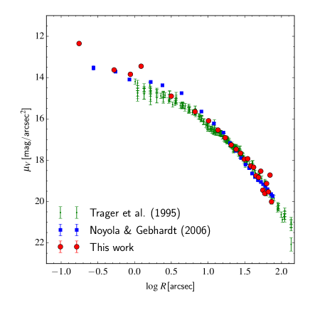
Figure 1: Comparison between the surface brightness profiles available in literature and the one derived in this work.

2.1.2 Kinematics

To constrain the mass of the GC, we use the one-dimensional velocity dispersion ($\sigma_{\rm pm}$) derived from HST proper motions presented in Watkins et al. (2015). These data include stars down to a magnitude 1 magnitude below the turn-off, and in the modelling we assume that all stars for which we have velocities have the same mass, equal to the turn-off mass. We adopt a distance to NGC 6624 of 7.9 kpc (Harris, 2010) to convert model velocities to observed proper motion units of mas/yr.

There are only a few line-of-sight velocity measurements available for stars in NGC 6624 (Pryor et al., 1989; Zaggia et al., 1992). The available data are not sufficient to provide significant constraints on the line-of-sight velocity dispersion profile ($\sigma_{\rm los}(R)$). We therefore do not include these data in the fitting, but compare our models to these data in Section 3.1. We note that Valenti, Origlia & Rich (2011) present high-resolution spectroscopy of five stars in NGC 6624, and report line-of-sight velocities, but do not quote uncertainties and we can therefore not use them.

2.2 Models

2.2.1 Dynamical models

We use the limepy family of dynamical models (Gieles & Zocchi, 2015), which are distribution function-based models that approximate isothermal spheres in the centre and have a polytropic truncation near the escape energy, making them suitable to describe dynamically evolved and tidally limited systems, such as GCs. The ‘sharpness’ of the truncation in energy is described by a parameter $g$, which relates to the polytropic index $n$ as $n=g+1.5$. The concentration of the model is determined by the dimensionless central potential $W_{0}$, similarly to what is done in King (1966) models (we note that isotropic limepy models with $g=1$ are indeed King models.). We adopt an isotropic velocity distribution, appropriate for GCs in the late stages of their evolution (Tiongco, Vesperini & Varri 2016; Zocchi et al. 2016). Multiple mass components can be included to describe the effect of mass segregation (as in Gunn & Griffin, 1979). The velocity scale of each mass component ($s_{j}$) relates to the mass of the component ($m_{j}$) as $s_{j}\propto m_{j}^{-1/2}$. Extensive testing of limepy against the results of direct $N$-body simulations was done by Zocchi et al. (2016) for single-mass models and Peuten et al. (2017) for multimass models. Of particular importance for this study is that limepy models accurately reproduce the degree of mass segregation in multimass systems. The meaning of the model parameter $W_{0}$ depends on the definition of the mean mass, for which two options are available in limepy. We use the global mean mass of the entire model, rather than the central density weighted mean mass, as is done in Gunn & Griffin (1979). We refer to Peuten et al. (2017) for a discussion on this choice.

2.2.2 Stellar-mass function

The multimass limepy models require as input a mass function (MF) for stars and remnants and for this we use the ‘evolved MF’ algorithm presented in Balbinot & Gieles (2017). It assumes a Kroupa (2001) stellar initial mass function (IMF), which is then evolved for 12 Gyr by applying the effect of mass loss by stellar evolution and remnant creation and the preferential escape of low-mass stars and remnants as the result of evaporation. Based on the orbit and the age of NGC 6624, Balbinot & Gieles (2017) estimate that the fraction of remaining cluster mass of NGC 6624 is $\mu=0.09\pm 0.02$. We explored various MFs for different values of $\mu$ and found good agreement with the observed stellar MF presented by Saracino et al. (2016) for $\mu=0.065$, which we use from hereon. We adopt a retention fraction of neutron stars of 5 per cent and assume that there are no stellar-mass black holes, as expected for core collapsed clusters (Breen & Heggie, 2013). We note that the MF is relatively insensitive to the adopted neutron star retention fraction, because the total mass fraction in neutron stars for 100 per cent retention is only 2 per cent. For this MF, the fraction of the total cluster mass in dark remnants is $0.62$. The MF of stars and stellar remnants is shown in Fig. 2. There are 10 mass bins for the stars, and five mass bins for the remnants, such that there are 15 components in the multimass model. For the stars, we convert mass to $V$-band luminosity using the flexible stellar population synthesis (FSPS) models of Conroy & Gunn (2010), adopting $Z=0.0049$ and an age of 12 Gyr.

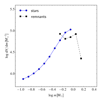
Figure 2: The evolved stellar MF used to set up the multimass dynamical model. Because the cluster is near dissolution, the MF is depleted in low-mass stars and $\sim 60$ per cent of the total mass resides in dark stellar remnants.

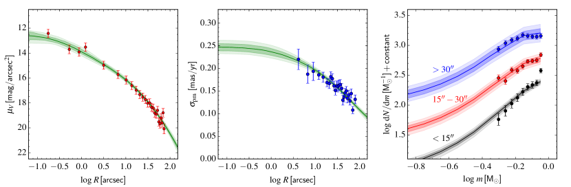
Figure 3: Comparison between the observational data of NGC 6624 and the dynamical models. The left panel shows the surface brightness profile, where the error bars are found from the (quadratic) sum of the uncertainty in the data and the nuisance parameter resulting from the fit: $\sigma_{\mu}\simeq 0.3\,{\rm mag}/{\rm arcsec}^{2}$. The one dimensional velocity dispersion is shown in the middle panel and the right panel shows the stellar MF in different radial bins. The three MFs are shifted with arbitrary constants for clarity.

2.3 Model fitting

With the MF defined, there are six fitting parameters: the limepy model parameters $W_{0}$ and $g$ and two physical scales of the cluster, for which we use $r_{\rm h}$ and the total cluster mass $M$. Additionally, we fit on the global mass-to-light ratio $\Upsilon_{V}$, which we use to scale the normalized luminosity profile to the surface brightness profile. In this way, $M$ is only constrained by the kinematics. Finally, we add a nuisance parameter $\sigma_{\mu}$ in quadrature to $\sigma_{V}$ to account for the effect of stochastic sampling of the stellar luminosity function. We adopt uniform priors for all parameters with the following range: $1\leq W_{0}\leq 12$, $0\leq g\leq 2.5$, $10^{4}\leq M/{\rm M}_{\odot}\leq 10^{6}$, $0.1\leq r_{\rm h}/{\rm pc}\leq 20$, $0<\Upsilon_{V}/({\rm M}_{\odot}/{\rm L}_{V,\odot})\leq 5$ and $0<\sigma_{\mu}\leq 1$. To determine the posterior distributions of the model parameters and best-fit values, we use the software package emcee (Foreman-Mackey et al., 2013), which is a pure-python implementation of the Goodman & Weare’s affine invariant Monte Carlo Markov Chain (MCMC) ensemble sampler (Goodman & Weare, 2010). We use 200 walkers and after a few hundred steps the fit converged. We continued for 2000 steps and in the analyses we use the final walker positions to generate posterior distributions and generate model properties. The python implementation of emcee makes it straightforward to couple it with limepy.

3 Results

3.1 Comparison to data and model parameters

The resulting surface brightness and velocity dispersion profiles of the models are compared to the data in the left and middle panels of Fig. 3, respectively. The median model values at each radius are depicted with lines, and the $1\sigma$ and $2\sigma$ spreads are shown with dark and light shaded (green) regions, respectively. The resulting stellar MFs at three distances from the GC centre are shown together with the data of Saracino et al. (2016) in the right panel. Note that we did not fit on the MF. The spread in the model MFs is the result of the variations in the model parameters, leading to different MFs in the three regions. The best-fit model parameters and corresponding uncertainties (i.e. the median and $1\sigma$ uncertainties) of the six parameters are given in Table 1.

Table 1: Summary of the fit results.

$W_{0}$	$g$	$M$	$r_{\rm h}$	$\Upsilon$	$\sigma_{\mu}$
		$[10^{5}\,{\rm M}_{\odot}]$	[pc]	$[{\rm M}_{\odot}/{\rm L}_{V,\odot}]$
$9.83_{-1.30}^{+1.10}$	$2.24_{-0.12}^{+0.18}$	$1.11_{-0.13}^{+0.12}$	$2.40_{-0.58}^{+0.42}$	$1.30_{-0.09}^{+0.09}$	$0.32_{-0.07}^{+0.05}$

Zaggia et al. (1992) measured $\sigma_{\rm los}$ in the centre of NGC 6624, using integrated light spectroscopy of the inner $8.4\arcsec\times 4.6\arcsec$ and find $\sigma_{\rm los}=8.9\pm 1.8\,{\rm km/s}$. Pryor et al. (1989) present velocities of 19 stars, of which 18 stars between $\sim 4\arcsec$ and $\sim 15\arcsec$ from the centre. We split these data in two samples of 9 stars (excluding their innermost isolated data point at $R\simeq 0.6\arcsec$), with respect to the median distance to the centre and determine $\sigma_{\rm los}$ from their line-of-sight velocities via a maximum likelihood method using emcee. The resulting dispersions from the Pryor et al. data at two locations and the Zaggia et al. measurement are compared to the velocity dispersion of our models in Fig. 4. The large uncertainties in the measured $\sigma_{\rm los}$ (relative to the proper motion dispersion, see Fig. 3) do not allow us to use $\sigma_{\rm los}$ to further constrain the model.

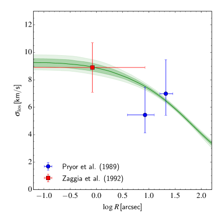
Figure 4: Line-of-sight velocity dispersion from the dynamical models compared to literature data.

3.2 Line-of-sight acceleration

For each model we determine the maximum acceleration along the line-of-sight as a function of distance to the centre in projection, $\max(a_{\rm los})$. The result is shown in Fig. 5, together with the acceleration of PSR B1820–30A as inferred from $\dot{P}/P$. The thick(thin) horizontal error bar shows the $1\sigma(2\sigma)$ uncertainties in the distance from the centre, due to the uncertain position of the cluster centre (see Section 2.1.1). Accounting for the uncertainties in the models and the pulsar position, $\max(a_{\rm los})$ of the models can accommodate for the acceleration derived from $\dot{P}/P$. Phinney (1993) showed that the maximum acceleration in the core is proportional to the central surface mass density ($\Sigma_{0}$), with $\max(a_{\rm los})/c\simeq 5\times 10^{-16}\,{\rm s}^{-1}$ for $\Sigma_{0}=10^{6}\,{\rm M}_{\odot}/{\rm pc}^{2}$. From the models we derive $\Sigma_{0}=1.86_{-0.90}^{+2.22}\times 10^{6}\,{\rm M}_{\odot}\,{\rm pc}^{-2}$, such that the observed $\dot{P}/P\simeq 6.2\times 10^{-16}\,{\rm s}^{-1}$ is comfortably below the expected maximum inside the core [$\max(a_{\rm los})/c\simeq 10^{-15}\,{\rm s}^{-1}$].

The central mass-to-light ratio in the $V$-band is $\Upsilon_{V,0}=5.47_{-1.60}^{+3.33}\,{\rm M}_{\odot}/{\rm L}_{V,\odot}$, larger than the global $\Upsilon_{V}\simeq 1.3\,{\rm M}_{\odot}/{\rm L}_{V,\odot}$ (see Table 1). This is because of the central concentration of dark remnants. From this we see that the pulsar acceleration can be explained by mass models, based on a canonical IMF evolved to an age of 12 Gyr for the effects of stellar evolution and the escape of low-mass stars (see Section 2.2.2 and Fig. 2 for details), without the need for an IMBH.

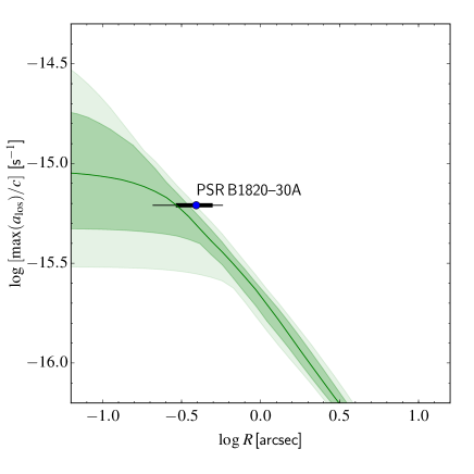
Figure 5: Comparison of the maximum acceleration along the line-of-sight as a function of distance to the centre in projection for the models and the inferred acceleration of PSR B1820–30A. The median result of the models is shown as a line and $1\sigma$ and $2\sigma$ spreads are shown as dark and light shaded regions. Within the $1\sigma$ uncertainty, the inferred acceleration of PSR B1820–30A can be accommodated by the enclosed mass profile of the cluster.

3.3 Discrete models

We quantify the effect of nearby passing stars and remnants on the spin derivatives by generating $10^{3}$ discrete realizations of the multimass models from randomly drawn walkers of the final MCMC chains. In each model we add $10^{3}$ mass-less tracers, at positions corresponding to PSR B1820–30A. We assign projected distances on a ring with radius $0.41\pm 0.09\arcsec$, assuming a Gaussian spread, and we sample positions along the line-of-sight from the density distribution of the neutron stars. We then use the expressions for the acceleration, jerk, snap and crackle from Nitadori & Makino (2008), to derive $P^{(n)}$, with $1\leq n\leq 4$, respectively. We omit $P^{(5)}$ because there is only an upper limit available.

In Fig. 6 we show the frequency ($\phi$) for each of the $P^{(n)}$ for the $10^{6}$ tracers. The regions containing $68\%$ of the points (i.e. between the 16 and 84 percentiles) are indicated with a (blue) shaded area. For $\dot{P}$, the distribution peaks near the maximum value, which means that it is more likely to find an acceleration near the maximum, than near 0.

The observed values for PSR B1820–30A (derived from the frequencies reported by Perera et al. 2017a) are indicated with an arrow in each panel. The $\dot{P}$ of PSR B1820–30A is slightly beyond the peak of the distribution, with $1.5\%$ of the tracer particles having $|\dot{P}|/P$ larger than observed. Blandford et al. (1987) showed that the typical contribution of passing stars to $\ddot{P}$ is of comparable magnitude as the contribution of the mean gravitational field and Phinney (1993) showed that this is also true for the higher-order derivatives. We confirm this here: the higher-order derivatives of PSR B1820–30A are within the $1\sigma$ spreads, implying that values of $P^{(n)}$ with $n\geq 2$ are dominated by stochastic effects and can not be used to infer the smooth underlying potential.

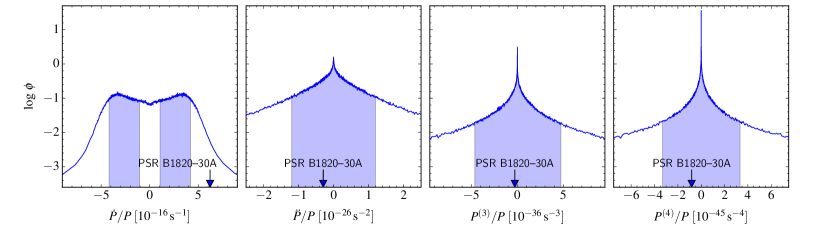
Figure 6: Frequency $\phi$ of $P$ derivatives from discrete realizations of the dynamical models. Observed values from timing observations of PSR B1820–30A by Perera et al. (2017a) are indicated with arrows. The shaded regions indicate the values between the 16 and 84 percentiles, around the most likely value(s).

By considering the correlations between $P^{(n)}$ with $n\geq 2$ and $\dot{P}$, we find that for the points with the largest $|\dot{P}|/P$, the higher-order derivatives are also near the maximum of their respective distributions. This is because the derivatives for these points are dominated by a single, nearby star rather than the global potential. For a value of $|\dot{P}|/P\simeq 6.2\times 10^{-16}\,{\rm s}^{-1}$, as found for PSR B1820–30A, the most likely values of $|P^{(n)}|/P$ for $n=[2,3,4]$ are roughly $[5\times 10^{-26}\,{\rm s}^{-2},5\times 10^{-35}\,{\rm s}^{-3},10^{-44}\,{\rm s}^{-4}]$, all well outside the $1\sigma$ regions indicated in Fig. 3. The observed values of $P^{(n)}$ with $n\geq 2$ are within the $1\sigma$ intervals of our models, which suggests that $\dot{P}$ is not the result of the acceleration due to a single, nearby star and an additional intrinsic spin-down contribution to $\dot{P}$ is required. For $|\dot{P}|/P\simeq 4\times 10^{-16}\,{\rm s}^{-1}$, the higher-order derivatives can have any value shown in the distributions in Fig. 6. This suggests that at least $\sim 30$ per cent of $\dot{P}$ is due to intrinsic spin-down. We discuss in Section 4 that such a contribution to $\dot{P}$ is not unreasonable given the high $\gamma$-ray luminosity of PSR B1820–30A. Such a contribution to $\dot{P}$ would also make the resulting line-of-sight acceleration easier to explain by our models, because $\sim 20$ per cent of our model points in the left panel of Fig. 6 have $|a_{\rm los}|/c\gtrsim 4\times 10^{-16}\,{\rm s}^{-1}$.

4 Conclusions and discussion

Perera et al. (2017a, b) conclude that an IMBH with $M_{\rm BH}\gtrsim 7\,500\,{\rm M}_{\odot}$ is required to explain the timing observations of the MSP in the core of NGC 6624. We have shown that $\dot{P}$ and higher-order derivatives of $P$ of PSR B1820–30A in NGC 6624 can be explained by dynamical multimass models without an IMBH. The models were derived from fits to the surface brightness and kinematics profiles of this GC. The best-fit dynamical models have central densities of $\rho_{0}=7.54_{-5.56}^{+34.3}\times 10^{7}\,{\rm M}_{\odot}\,{\rm pc}^{-3}$ and a central surface density of $\Sigma_{0}=1.96_{-0.98}^{+2.51}\times 10^{6}\,{\rm M}_{\odot}\,{\rm pc}^{-2}$, which explains the high acceleration of the MSP near the centre. Although these central densities are high, they are in the range expected for core-collapsed clusters. For example, den Brok et al. (2014) find $\rho_{0}\simeq 3\times 10^{7}\,{\rm M}_{\odot}\,{\rm pc}^{-3}$ in Jeans models of M15. Similar values have also been found in evolutionary models of core-collapsed clusters: Grabhorn et al. (1992) modelled NGC 6624 with Fokker–Planck models and find $\rho_{0}\simeq 2\times 10^{7}\,{\rm M}_{\odot}\,{\rm pc}^{-3}$, which combined with their core radius of $r_{0}\simeq 0.05\,{\rm pc}$ gives rise to $\Sigma_{0}=\rho_{0}r_{0}\simeq 10^{6}\,{\rm M}_{\odot}\,{\rm pc}^{-3}$. Similar results were obtained with Fokker–Planck models of M15 (Murphy, Cohn & Lugger, 2011) and $N$-body models of NGC 6397 (Heggie & Giersz, 2009). We note that the enclosed mass within the radius of the MSP is lower than the inferred IMBH mass of Perera et al. (2017a): $M(<0.41\arcsec)=646_{-163}^{+74}\,{\rm M}_{\odot}$ (and in three dimensions: $M(<0.41\arcsec)=362_{-199}^{+93}\,{\rm M}_{\odot}$). We therefore agree with the conclusion of Peuten et al. (2014) that NGC 6624 has a population of centrally concentrated dark remnants. However, these authors did not present dynamical models. They varied the inner (mass) density profile with respect to the light profile to obtain a central mass profile that could fully explain $\dot{P}_{\rm orb}$ of 4U 1820–30 by the line-of-sight acceleration. Their $\Upsilon_{V}(R)$ starts to significantly increase within $R\lesssim 5\arcsec$, whereas in our models $\Upsilon_{V}(R)$ rises only within $R\lesssim 1\arcsec$ (see Fig. 7). The line-of-sight acceleration of our models at the position of 4U 1820–30 ($R\simeq 1.3\arcsec$) is therefore not able to explain $\dot{P}_{\rm orb}$ of 4U 1820–30. New analyses show that the LMXB may be closer to the centre of the cluster (Jay Strader, private communication; Tremou et al., in preparation), but even if it resides as close to the centre of NGC 6624 as PSR B1820–30A, only $\sim 30$ per cent of $\dot{P}_{\rm orb}$ would be due to a gravitational acceleration. More importantly, as we argued in Section 1, there are LMXBs in the field with similar (or higher) $|\dot{P}_{\rm orb}|$, which is why we do not interpret this signal as being the result of an acceleration.

Our global mass-to-light ratio $\Upsilon_{V}=1.30\pm 0.09\,{\rm M}_{\odot}/{\rm L}_{V,\odot}$ is lower than what is expected from stellar population models. From the FSPS models (Conroy & Gunn, 2010) we estimate $\Upsilon_{V}\simeq 2.88\,{\rm M}_{\odot}/{\rm L}_{V,\odot}$, for a stellar population with an age of 12 Gyr, $Z=0.0049$ and a Kroupa (2001) IMF. The difference is because NGC 6624 is depleted in low-mass stars (see the right panel in Fig. 3) as the result of dynamical evolution in the Galactic tidal field. By matching the present-day MF of the FSPS model to the observed MF, we obtain $\Upsilon_{V}=1.15\,{\rm M}_{\odot}/{\rm L}_{V,\odot}$, close to what we infer from the mass models. This agreement lends further support to the validity of the best-fit multimass models.

Our results depend on the distance $D$, for which we adopted $D=7.9$ kpc (Harris, 2010). The model properties depend on $D$ in the following way: the velocity dispersion in [km/s] derived from the proper motions and $r_{\rm h}$ in [pc] both depend linearly on $D$. From virial equilibrium arguments, the total dynamical mass is proportional to $\sigma^{2}r_{\rm h}\propto D^{3}$. The surface density (and therefore the line-of-sight acceleration; see Section 3.2 and Phinney, 1993), scales as $D$. The inferred $\max(a_{\rm los})$ is therefore also proportional to $D$. With line-of-sight velocities beyond $\gtrsim 3\arcsec$ a dynamical distance to NGC 6624 can be obtained. Improved line-of-sight velocities of stars within $\lesssim 3\arcsec$, i.e. where there are no proper motions available, would also be helpful to place tighter constraints on the mass profiles in the centre (Richstone & Tremaine, 1986).

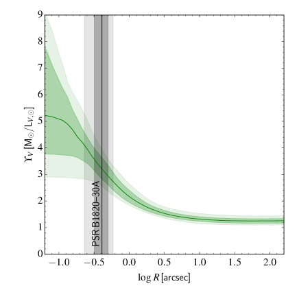
Figure 7: Mass-to-light ratio profile from the dynamical models. The location of PSR B1820–30A  and corresponding $1\sigma$ and $2\sigma$ uncertainties are indicated with a vertical line and (black) shaded regions, respectively.

From randomly selecting walkers from the MCMC chain and populating the density profile of the neutrons stars with mass-less tracers, we find that in about 1.5 per cent of cases the line-of-sight acceleration is higher than what is inferred for PSR B1820–30A. Although this is suggestive that the model (surface) densities are on the low-side to account for the pulsar $\dot{P}$, we note that there is a contribution to the observed $\dot{P}$ from intrinsic spin-down due to magnetic breaking that we have so far not discussed. The $\gamma$-ray data of Freire et al. (2011) show that PSR B1820–30A dominates the $\gamma$-ray emission from NGC 6624. In fact, PSR B1820–30A is the most luminous $\gamma$-ray MSP known. Freire et al. (2011) estimate from the $\gamma$-ray emission that at least $10$ per cent of the observed $\dot{P}$ is due to the intrinsic spin-down, when one assumes an unrealistic $\gamma$-ray efficiency of $\eta=1$. If one assumes a more realistic efficiency of $\eta\simeq 0.1$ (Freire et al., 2011), the majority of the observed $\dot{P}$ could in fact be due to intrinsic effects.

There are five more pulsars known in NGC 6624 (Lynch et al., 2012), and for two of these there are $\dot{P}$ measurements. Both have $P\simeq 0.4\,{\rm s}$, and their $\dot{P}$ values are comparable to what is found for pulsars in the field with similar $P$ (Manchester et al., 2005), implying that these pulsars can not be used to infer the gravitational potential.

MSPs are potentially the only way of inferring the acceleration with sufficient precision to make a viable case for an IMBH. To form a MSP, a pulsar needs to tidally capture a star, which subsequently spins up the pulsar by angular momentum transport via Roche overflow (Verbunt et al., 1987). However, high stellar densities are required for tidal capture to be efficient (Fabian et al., 1975), and an IMBH reduces the stellar density (Heggie et al., 2007), making GCs with MSPs unlikely GCs to possess an IMBH. Given the degeneracies of a dynamical signal of an IMBH with radial velocity anisotropy (Zocchi et al., 2017b) and the presence of a stellar-mass black hole population (Lützgendorf et al., 2013; Peuten et al., 2016; Zocchi et al., 2017a), perhaps a convincing detection will need to come from gravitational microlensing (Kains et al., 2016). Future instrumentation, such as the ELT first-light instrument MICADO (Davies et al., 2010), may be able to resolve the proper motion velocity dispersion to sufficiently close distances to the centre of clusters and for enough stars to be able to find convincing signatures of IMBHs in the cores of GCs, if they exist.

References

- Anderson & van der Marel (2010) Anderson J., van der Marel R. P., 2010, ApJ, 710, 1032
- Balbinot & Gieles (2017) Balbinot E., Gieles M., 2017, MNRAS accepted, arXiv:1702.02543
- Baumgardt et al. (2004) Baumgardt H., Makino J., Ebisuzaki T., 2004, ApJ, 613, 1143
- Bianchini et al. (2016) Bianchini P., van de Ven G., Norris M. A., Schinnerer E., Varri A. L., 2016, MNRAS, 458, 3644
- Blandford et al. (1987) Blandford R. D., Romani R. W., Applegate J. H., 1987, MNRAS, 225, 51P
- Breen & Heggie (2013) Breen P. G., Heggie D. C., 2013, MNRAS, 432, 2779
- Claydon et al. (2017) Claydon I., Gieles M., Zocchi A., 2017, MNRAS, 466, 3937
- Conroy & Gunn (2010) Conroy C., Gunn J. E., 2010, ApJ, 712, 833
- Daniel et al. (2017) Daniel K. J., Heggie D. C., Varri A. L., 2017, MNRAS, 468, 1453
- Davies et al. (2010) Davies R., et al., 2010, Proc. SPIE, 7735, 77352A
- den Brok et al. (2014) den Brok M., van de Ven G., van den Bosch R., Watkins L., 2014, MNRAS, 438, 487
- Djorgovski & King (1986) Djorgovski S., King I. R., 1986, ApJ, 305, L61
- Eisenhauer et al. (2005) Eisenhauer F., et al., 2005, ApJ, 628, 246
- Fabian et al. (1975) Fabian A. C., Pringle J. E., Rees M. J., 1975, MNRAS, 172, 15p
- Ferrarese & Merritt (2000) Ferrarese L., Merritt D., 2000, ApJ, 539, L9
- Foreman-Mackey et al. (2013) Foreman-Mackey D., Hogg D. W., Lang D., Goodman J., 2013, PASP, 125, 306
- Freire et al. (2011) Freire P. C. C., et al., 2011, Science, 334, 1107
- Fukushige & Heggie (2000) Fukushige T., Heggie D. C., 2000, MNRAS, 318, 753
- Gieles & Zocchi (2015) Gieles M., Zocchi A., 2015, MNRAS, 454, 576
- Gill et al. (2008) Gill M., Trenti M., Miller M. C., van der Marel R., Hamilton D., Stiavelli M., 2008, ApJ, 686, 303
- Goldsbury et al. (2010) Goldsbury R., Richer H. B., Anderson J., Dotter A., Sarajedini A., Woodley K., 2010, AJ, 140, 1830
- Goodman & Weare (2010) Goodman J., Weare J., 2010, Commun. Appl. Math. Comput. Sci., 5, 65
- Grabhorn et al. (1992) Grabhorn R. P., Cohn H. N., Lugger P. M., Murphy B. W., 1992, ApJ, 392, 86
- Gunn & Griffin (1979) Gunn J. E., Griffin R. F., 1979, AJ, 84, 752
- Harris (2010) Harris W. E., 2010, ArXiv:1012.3224,
- Heggie & Giersz (2009) Heggie D. C., Giersz M., 2009, MNRAS, 397, L46
- Heggie et al. (2007) Heggie D. C., Hut P., Mineshige S., Makino J., Baumgardt H., 2007, PASJ, 59, L11
- Illingworth & King (1977) Illingworth G., King I. R., 1977, ApJ, 218, L109
- Kains et al. (2016) Kains N., Bramich D. M., Sahu K. C., Calamida A., 2016, MNRAS, 460, 2025
- King (1966) King I. R., 1966, AJ, 71, 64
- Kroupa (2001) Kroupa P., 2001, MNRAS, 322, 231
- Lanzoni et al. (2013) Lanzoni B., et al., 2013, ApJ, 769, 107
- Leonard (1991) Leonard P. J. T., 1991, AJ, 101, 562
- Lützgendorf et al. (2011) Lützgendorf N., Kissler-Patig M., Noyola E., Jalali B., de Zeeuw P. T., Gebhardt K., Baumgardt H., 2011, A&A, 533, A36
- Lützgendorf et al. (2012) Lützgendorf N., et al., 2012, A&A, 543, A82
- Lützgendorf et al. (2013) Lützgendorf N., Baumgardt H., Kruijssen J. M. D., 2013, A&A, 558, A117
- Lynch et al. (2012) Lynch R. S., Freire P. C. C., Ransom S. M., Jacoby B. A., 2012, ApJ, 745, 109
- Manchester et al. (2005) Manchester R. N., Hobbs G. B., Teoh A., Hobbs M., 2005, AJ, 129, 1993
- Meylan et al. (1991) Meylan G., Dubath P., Mayor M., 1991, ApJ, 383, 587
- Murphy et al. (2011) Murphy B. W., Cohn H. N., Lugger P. M., 2011, ApJ, 732, 67
- Newell et al. (1976) Newell B., Da Costa G. S., Norris J., 1976, ApJ, 208, L55
- Nitadori & Makino (2008) Nitadori K., Makino J., 2008, New Astron, 13, 498
- Noyola & Gebhardt (2006) Noyola E., Gebhardt K., 2006, AJ, 132, 447
- Noyola et al. (2008) Noyola E., Gebhardt K., Bergmann M., 2008, ApJ, 676, 1008
- Patruno et al. (2017) Patruno A., et al., 2017, ApJ, 841, 98
- Perera et al. (2017a) Perera B. B. P., et al., 2017a, MNRAS, 468, 2114
- Perera et al. (2017b) Perera B. B. P., et al., 2017b, MNRAS, 471, 1258
- Peuten et al. (2014) Peuten M., Brockamp M., Küpper A. H. W., Kroupa P., 2014, ApJ, 795, 116
- Peuten et al. (2016) Peuten M., Zocchi A., Gieles M., Gualandris A., Hénault-Brunet V., 2016, MNRAS, 462, 2333
- Peuten et al. (2017) Peuten M., Zocchi A., Gieles M., Hénault-Brunet V., 2017, MNRAS, 470, 2736
- Phinney (1993) Phinney E. S., 1993, in Djorgovski S. G., Meylan G., eds, Astronomical Society of the Pacific Conference Series Vol. 50, Structure and Dynamics of Globular Clusters. p. 141
- Pryor et al. (1989) Pryor C., McClure R. D., Fletcher J. M., Hesser J. E., 1989, AJ, 98, 596
- Richstone & Tremaine (1986) Richstone D. O., Tremaine S., 1986, AJ, 92, 72
- Saracino et al. (2016) Saracino S., et al., 2016, ApJ, 832, 48
- Strader et al. (2012) Strader J., Chomiuk L., Maccarone T. J., Miller-Jones J. C. A., Seth A. C., Heinke C. O., Sivakoff G. R., 2012, ApJ, 750, L27
- Tiongco et al. (2016) Tiongco M. A., Vesperini E., Varri A. L., 2016, MNRAS, 455, 3693
- Trager et al. (1995) Trager S. C., King I. R., Djorgovski S., 1995, AJ, 109, 218
- Valenti et al. (2011) Valenti E., Origlia L., Rich R. M., 2011, MNRAS, 414, 2690
- Verbunt et al. (1987) Verbunt F., van den Heuvel E. P. J., van Paradijs J., Rappaport S. A., 1987, Nature, 329, 312
- Watkins et al. (2015) Watkins L. L., van der Marel R. P., Bellini A., Anderson J., 2015, ApJ, 803, 29
- Zaggia et al. (1992) Zaggia S. R., Capaccioli M., Piotto G., Stiavelli M., 1992, A&A, 258, 302
- Zocchi et al. (2016) Zocchi A., Gieles M., Hénault-Brunet V., Varri A. L., 2016, MNRAS, 462, 696
- Zocchi et al. (2017a) Zocchi A., Gieles M., Hénault-Brunet V., 2017a, submitted
- Zocchi et al. (2017b) Zocchi A., Gieles M., Hénault-Brunet V., 2017b, MNRAS, 468, 4429