Careful prior specification avoids incautious inference for log-Gaussian Cox point processes

Abstract

Prior specifications for hyperparameters of random fields in Bayesian spatial point process modelling can have a major impact on the statistical inference and the conclusions made. We consider fitting of log-Gaussian Cox processes to spatial point patterns relative to spatial covariate data. From an ecological point of view, an important aim of the analysis is to assess significant associations between the covariates and the point pattern intensity of a given species. This paper introduces the use of a reparameterised model to facilitate meaningful interpretations of the results and how these depend on hyperprior specifications. The model combines a scaled spatially structured field with an unstructured random field, having a common precision parameter. An additional hyperparameter identifies the fraction of variance explained by the spatially structured term and proper scaling makes the analysis invariant to grid resolution. The hyperparameters are assigned penalised complexity priors, which can be tuned intuitively by user-defined scaling parameters. We illustrate the approach analysing covariate effects on point patterns formed by two rainforest tree species in a study plot on Barro Colorado Island, Panama.

Keywords: Bayesian inference, ecological point process, penalised complexity prior, R-INLA, spatial modelling

1 Introduction

1.1 Habitat association modelling

There is a strong ecological interest in understanding the mechanisms that allow different species to coexist within an ecosystem, and in particular in extremely species-rich systems, such as rainforests or coral reefs (Chesson, 2000; Hubbell, 2001; Dornelas et al., 2006). Habitat association has often been seen as a potential strategy that reduces interspecific competition and hence facilitates coexistence (Connell, 1961; Bagchi et al., 2011). Ecological research has highlighted associations of specific plant species with distinct habitat defined by, for instance, climate and soil, but in many cases these associations have been derived from anecdotal knowledge expressed in floras rather than from a study that has thoroughly tested them. Recently, increasingly detailed data on soil properties have become available which provide fine-scale, spatially continuous data on soil chemistry rather than discrete habitat types providing an opportunity for a more detailed and local analysis characterising a species’ environmental preferences.

A statistical analysis of the relevant data structure here would need to relate the individuals’ occurrence in a specific location to the local environment. Spatial point process methodology (Diggle, 2003; Illian et al., 2008; Baddeley et al., 2015) has been used in this context (Law et al., 2009; Wiegand and Moloney, 2014; Velázquez et al., 2016) as it models the pattern formed by individuals in space relative to local conditions. Common approaches relate the occurrence of an individual in a location in continuous space to a set of environmental covariates. In addition to the terms representing these spatial covariates and associated parameters, models contain a further term, for instance a spatially structured random field such as a Gaussian random field, which accounts for spatial structures unexplained by the covariates (Illian et al., 2012a; Waagepetersen et al., 2016). These structures might be the result of biotic mechanisms such as dispersal limitation or of unobserved covariates.

However, this modelling approach is not as straight forward as it might seem. In particular, the literature is lacking a thorough discussion of (a) the impact of the smoothness of the spatial field on inference and (b) complexity of accounting for unexplained spatial structures due to mechanisms operating at a number of spatial scales. With regard to (a), the level of significance of the covariates’ association with the observed spatial pattern in a fitted model is not independent of the smoothness of the spatially structured field, and determining this smoothness in an objective way is difficult, see Section 1.2. Furthermore, the remaining spatial structure is likely to operate at different spatial scales, e.g.  as a combination of large scale clustering due to habitat association and small scale clustering due to local dispersal, and these are difficult to disentangle (Hamill and Wright, 1986; Bagchi et al., 2011). In both the statistical literature on point processes and the ecological literature using spatial point process methods these issues have not been explicitly resolved. To the best of our knowledge a discussion of principles for choosing the smoothness of the spatial field is entirely absent from the spatial point process literature with a few papers accounting for the issue of clustering at different spatial scales (John et al., 2007; Illian et al., 2012a; Shen et al., 2013).

In this paper, we acknowledge these issues and that there is no universal objective criterion for resolving them. We discuss Bayesian methodology that allows us to investigate the spatial behaviour by a) constructing a model that explicitly takes the awareness of these issues into account and b) suggesting a constructive way of addressing them. This is done by using interpretable priors that allow us to vary the focus on different spatial scales and to observe changes in the resulting estimates with changes in scale. In other words we do not attempt to identify a single degree of smoothing that is optimal by some criterion but consider a standardised range of degrees of smoothing and observe the behaviour of the estimates relative to changes in smoothness.

The approach discussed here has been motivated by the analysis of point patterns formed by tropical forest tree species within the 50-ha rectangular plot at Barro Colorado Island (BCI), Panama. This plot was designed to help address the mechanisms that maintain species richness and deliberately involved spatial mapping of the entire community following the recognition that population and community dynamics occur in a spatial context (Hubbell, 2001). The full dataset includes observed positions for a large number of tree species (Condit, 1998; Hubbell et al., 1999, 2005) and measurements of topographical variables and soil nutrients that potentially influence the spatial distribution of the trees (John et al., 2007; Schreeg et al., 2010). A main aim of the statistical analysis is to investigate whether the spatial patterns of different tree species can be related to spatial environmental variations, reflected by observed topography and soil nutrients (Møller and Waagepetersen, 2007). To appropriately inform model choice and inference, this paper suggests an approach that does neither attempt to universally suggest an optimal degree of smoothing nor to a fixed spatial scale at which mechanisms are operating. This is done by explicitly communicating prior choices that impact on inference and statistical conclusions.

1.2 The statistical perspective

Point pattern data are the observed locations of objects or events within a bounded geographical region, for example the locations of plants or animals in the wild or the locations of earthquakes. By fitting a spatial point process model, the spatial structure of the pattern can be studied in terms of observed environmental variables that are included as covariates. To perform reliable statistical inference and to make an honest accounting of estimation uncertainty, it is of vital importance to also account for spatial dependence structures and random error due to potentially missing covariates and biotic processes. The resulting model will be sensitive to input choices. Hence, extra effort must be made to correctly communicate statistical statements and conclusions.

This paper explicitly focuses on how hyperprior specifications influence the statistical inference when a discretized log-Gaussian Cox process (Møller et al., 1998) is fitted to an observed spatial point pattern, including covariate information. However, all of the conclusions in this paper remain valid for any point process model that includes a high- or infinite-dimensional parameter as well as covariates. A log-Gaussian Cox process is a Poisson process with random intensity $\Lambda(s)=\exp\{\eta(s)\},$ where $\{\eta(s):s\in\mathbb{R}^{2}\}$ is a latent Gaussian random field. To assess the influence of observed covariates, we can express the log-intensity $\eta(s)$ in a spatial grid cell $s$ as

$$\eta(s)=\beta_{0}+\sum_{j=1}^{n_{\beta}}\beta_{j}z_{j}(s)+u(s)+v(s),\quad s\in\Omega,$$ (1)

where $\Omega$ represents a bounded two-dimensional study region. Here, $\beta_{0}$ is an intercept while $\{\beta_{j}\}_{j=1}^{n_{\beta}}$ represent linear fixed effects of observed covariates $\{z_{j}(s),s\in\Omega\}_{j=1}^{n_{\beta}}$. The spatially-correlated random field $\boldsymbol{u}=\{u(s),\,s\in\Omega$} is included to account for spatial autocorrelation or over-dispersion in point counts among neighbouring grid cells. The random field $\boldsymbol{v}=\{v(s),\,s\in\Omega$} is referred to as an error field or a spatially unstructured effect, accounting for over-dispersion or clustering within grid cells. A common modelling strategy is to assign Gamma priors to the precision (inverse variance) parameters of the two random fields (Rue et al., 2009; Illian et al., 2012a, b; Kang et al., 2015). However, both the model formulation in (1) and the use of Gamma priors are burdened with problems:

1. The two random fields in the model are not independent as $\boldsymbol{v}$ can be seen to be included in $\boldsymbol{u}$ in situations with no spatial dependence. The priors for the precision parameters should therefore not be chosen independently (Simpson et al., 2017).

2. The model is highly sensitive to prior choices for the precision parameters, especially the input parameters for the precision of the spatial field (Illian et al., 2012b; Beguin et al., 2012; Sørbye and Rue, 2014; Papoila et al., 2014; Homburger et al., 2015). These are not easily controlled using traditional hyperpriors, like Gamma distributions.

3. If the spatial component is intrinsic, the model gives different degrees of smoothing for different grid resolutions and priors have to be adjusted if the grid resolution is changed (Sørbye and Rue, 2014).

To address these problems, we suggest a subjective, application-driven approach which facilitates clear interpretation of model components and hyperprior specifications. This paper introduces the use of a reparameterised model for log-Gaussian Cox processes, where the log-intensity is expressed by

$$\eta(s)=\beta_{0}+\sum_{j=1}^{n_{\beta}}\beta_{j}z_{j}(s)+\frac{1}{\sqrt{\tau}}\left(\sqrt{\phi}u^{*}(s)+\sqrt{1-\phi}v(s)\right),\quad\phi\in(0,1).$$ (2)

Here, $\boldsymbol{u}^{*}=\{u^{*}(s),\,s\in\Omega\}$ represents a scaled spatial random field, and the hyperparameters $\tau$ and $\phi$ are assigned penalised complexity (PC) priors (Simpson et al., 2017). We detail below why this modelling approach has important advantages and avoids the three problems listed above.

First, the identifiability issue between the spatially structured and unstructured fields is avoided, combining the two fields as one random component with a marginal variance governed by a common precision parameter $\tau$. Conditioned on $\tau$, the parameter $\phi$ helps the interpretation, as it explains how much of the random variation is attributed to the spatial term. The two hyperparameters $\tau$ and $\phi$ are then seen to have orthogonal interpretation, which makes it natural to choose the hyperpriors for these parameters independently, see Simpson et al. (2017) and Riebler et al. (2016) for a similar formulation for the BYM-model (Besag et al., 1991). This makes hyperprior selection transparent and we avoid tuning two precision parameters.

The second issue to consider is prior sensitivity. Prior choices for hyperparameters in Bayesian hierarchical models are crucial as these govern the variability and strength of dependence for the underlying latent field. Especially, sensitivity to hyperprior choices for precision parameters of random effects represents a major challenge (Roos and Held, 2011) and commonly used Gamma priors are not necessarily appropriate (Lunn et al., 2009). The prior choice for the precision parameter $\tau$ in (2) will have a major influence on posterior results and it is essential that we are able to interpret the results in terms of prior information. This is facilitated using the framework of PC priors (Simpson et al., 2017), in which the informativeness of hyperpriors are adjusted in an intuitive way by user-defined scaling parameters. Klein and Kneib (2016) found that PC priors have better empirical performance than other standard choices in a similar context.

Thirdly, the spatial field $\boldsymbol{u}^{*}$ in (2) needs to be scaled to ensure that a given prior for its precision yields the same degree of smoothness for different grid resolutions. This is automatically the case for Gaussian (Markov) random field priors (Cressie, 1993; Rue and Held, 2005). However, if the spatial model is intrinsic, the marginal variance will depend on the grid resolution and the model needs to be scaled to give a unified interpretation for its precision parameter. One approach to avoid this issue is to scale the model in terms of its generalized variance (Sørbye and Rue, 2014).

Figure 1: The point pattern formed by the species Calophyllum Longifolium (left) and Oenocarpus mapoura (right) observed in a 50-ha study plot on Barro Colorado Island, Panama.

To initially illustrate our point, consider the point patterns formed by the species Calophyllum longifolium (1461 trees) and Oenocarpus mapoura (2027 trees) (Figure 1), using the 2005 census of the BCI data. Figure 2 illustrates the posterior $95\%$ point-wise credible intervals for each of a number of selected covariates included as fixed effects in (2). Using an ordinary generalized linear model (GLM) with only fixed effects, all of the covariates are significant (black intervals). However, the variance is underestimated giving too narrow credible intervals as spatial autocorrelation is ignored. When the random field component is included, it is essential that the hyperprior specifications can be controlled and the implication on the interpretation of the model are well-understood as these govern the statistical conclusions made, as is clear from the figure. This is achieved using a range of hyperprior models for $\tau$, governed by a scaling parameter which prescribes a maximum value for the marginal standard deviation $\sigma=\tau^{-1/2}$ (see Section 2).

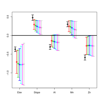
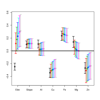
Figure 2: The posterior mean and $95\%$ point-wise credible intervals for the linear effects of fixed covariates for Calophyllum longifolium (left) and Oenocarpus mapoura (right). The black intervals show results using an ordinary generalized linear model with only linear effects of the covariates. For the other intervals, the PC prior for $\tau$ in (2) is scaled in terms of a user-defined scaling parameter $U_{\sigma}$, prescribing a maximum value for the marginal standard deviation $\tau^{-1/2}$, here using $U_{\sigma}=0.05$ (red), $U_{\sigma}=0.10$ (green), $U_{\sigma}=0.20$ (blue), $U_{\sigma}=0.5$ (cyan), $U_{\sigma}=1.0$ (purple) and $U_{\sigma}=2.0$ (grey).

Further details on the modelling approach taken here are given in Section 2, including scaling, computation and tuning of hyperpriors, and specifications for running the proposed model in the R-package R-INLA. Section 3 contains a thorough discussion on fitting the proposed model to the given example pattern, including interpretations of covariate associations and the posterior random fields. Discussion and concluding remarks are given in Section 4. A brief review on the principles underlying computation of penalised complexity priors is given in Appendix 5.

2 Modelling details

Log-Gaussian Cox processes may be interpreted as latent Gaussian models (Rue et al., 2009) where the observations are conditionally independent, given a latent Gaussian field $\boldsymbol{\eta}=\{\eta(s),\,s\in\Omega\}$. Here, we consider the case where the bounded observation window $\Omega$ is gridded and the set $\{y_{i}\}_{i=1}^{n}$ denotes the number of points in $n$ grid cells $\{s_{i}\}_{i=1}^{n}$. The conditional distribution of the counts is then assumed to approximately follow a Poisson distribution, i.e.,

$$y_{i}|\eta(s)\sim\mbox{Poisson}\left(\int_{s_{i}}\exp(\eta(s))ds\right)\approx\mbox{Poisson}(|s_{i}|\exp(\eta(s_{i}))).$$ (3)

The area of a grid cell is $|s_{i}|$ and $\eta(s_{i})$ denotes a representative value of the point log-intensity in cell $s_{i}$. Since the latent field $\eta(.)$ may be chosen flexibly, log-Gaussian Cox processes can be extended to analyse complex spatial point patterns, for example replicated point patterns and point patterns with marks (Illian et al., 2012a, b, 2013), and also to non-regular data (Simpson et al., 2016). However, the fitting of these models involves challenges, especially in terms of how hyperprior assumptions influence the inference. Unless we can communicate the meaning and interpretation of the role of priors for the hyperparameters, we cannot appropriately communicate the role of the latent model itself.

2.1 Spatial field specifications including scaling

Consider the case where the spatially structured field $\boldsymbol{u}=(u_{1},\ldots,u_{n})$ in (2) is an intrinsic conditional auto-regressive (ICAR) model (Besag et al., 1991). This prior is commonly applied to model underlying spatial dependence structures between neighbouring observations in Bayesian hierarchical models (Banerjee et al., 2004; Assunção and Krainski, 2009). The ICAR models are not proper but have several beneficial properties (Besag and Kooperberg, 1995). Especially, these models fit very nicely within the framework of PC priors as the models can be seen to penalise local deviation from their null space, as explained below.

Specifically, consider the ICAR prior defined on a regular lattice, also referred to as a second-order intrinsic Gaussian Markov random field (IGMRF) (Rue and Held, 2005, Section 3.4.2). The density of this model is defined by

$$\pi(\boldsymbol{u}\mid\tau_{u})\propto\tau_{u}^{\frac{1}{2}(n-2)}\exp{\left(-\frac{1}{2}\boldsymbol{u}^{T}\boldsymbol{Q}\boldsymbol{u}\right)},$$ (4)

where the precision matrix $\boldsymbol{Q}=\tau_{u}\boldsymbol{R}$. The parameter $\tau_{u}$ denotes the precision while $\boldsymbol{R}$ reflects the specific neighbourhood structure of the model. The precision matrix is singular of rank $n-2$ and does not specify an overall value for the mean, nor a finite variance. This is not a problem, as one can impose linear constraints to make the variance finite and the model then specifies a valid joint density. In fact, the rank deficiency implies that the null space of the model is a plane (Rue and Held, 2005) and the given model penalises local deviation from this plane. The marginal variances of the model, integrating out the random precision $\tau_{u}$, give information on how large we allow this local deviation to be. This implies that the hyperprior for $\tau_{u}$ has a clear interpretation, at least for a given model of a specified dimension.

An important feature of the IGMRF model which has usually not been accounted for in spatial point process analysis (Rue et al., 2009; Illian et al., 2012a, b, 2013; Kang et al., 2014), is that the marginal variances of the model depend on both the size and structure of $\boldsymbol{R}$ (Sørbye and Rue, 2014). This implies that a chosen prior for $\tau_{u}$ gives different degrees of smoothing, for different grid resolutions. To ensure a unified interpretation of the precision parameter $\tau_{u}$, the model $\boldsymbol{u}$ needs to be scaled. One way to do this is to consider the generalized variance of $\boldsymbol{u}$, computed as the geometric mean

$$\sigma^{2}_{\mbox{\scriptsize{GV}}}(\boldsymbol{u})=\frac{1}{\tau_{u}}\exp\left(\frac{1}{n}\sum_{i=1}^{n}\log(\sigma^{2}_{ii})\right),$$

where $\sigma^{2}_{ii}$ are the diagonal elements of the generalized inverse of $\boldsymbol{R}$ (Sørbye and Rue, 2014). The generalized variance can be seen to represent a characteristic or typical level for the marginal variances. For the given second-order IGMRF on a lattice, this generalized variance will increase by a factor of $k^{2}$ if the resolution for a study region is refined from $n\times n$ to $kn\times kn$ grid cells (Lindgren et al., 2011). By scaling $\boldsymbol{R}$ to have a generalized variance equal to 1 (Sørbye and Rue, 2014), the hyperprior for $\tau_{u}$ is invariant to grid resolution.

2.2 Tuning hyperparameters using PC priors

By using a scaled IGMRF-model $\boldsymbol{u}^{*}$, the random field component in (2), defined by

$$\psi(s)=\frac{1}{\sqrt{\tau}}\left(\sqrt{\phi}u^{*}(s)+\sqrt{1-\phi}v(s)\right)$$ (5)

is also scaled. This ensures that the precision parameter $\tau$ of the reparameterised model component has the same interpretation for different grid resolutions. Obviously, the grid resolution can still have a minor influence on the results as grid resolution impacts on the accuracy of the Poisson approximation in (3), where a very fine resolution yields a more accurate approximation than a coarser resolution. However, the higher the resolution the higher the required computation time – a trade-off that is relevant in practice. This will be discussed further for the given data example in Section 3.

The parameter $\tau$ represents the marginal precision of the random field component, and the prescribed size of this random effect is governed by the hyperprior specifications for $\tau$. Further, for a given finite precision, $\phi\in(0,1)$ can be interpreted as a mixing parameter which blends in spatial dependence in the model. As the two hyperparameters $\tau$ and $\phi$ control different features of the fitted random field, it is natural to assign independent hyperpriors to these parameters.

To facilitate control and interpretation of hyperprior choices, we use the recently developed framework of PC priors (Simpson et al., 2017). A main idea in calculating PC priors is that a random component, as in (5), can be seen as a flexible version of a simpler base model. An exponential prior is then assigned to a univariate measure of deviance from the flexible model to the simpler model, and transformed to give the PC prior for the parameter of interest. An important motivation for the given reparameterisation is to provide a proper sequence of base models, which can be used to derive PC priors for the hyperparameters $\phi$ and $\tau$, separately. Here, the simplest base model is one with no random effect, which corresponds to infinite precision $\tau$. This implies that given the covariates the pattern exhibits complete spatial randomness as represented by a homogeneous Poisson process. For a finite value of $\tau$, an alternative base model is defined as having no spatially structured effect ($\phi=0$). This could for example correspond to over-dispersed point patterns, where over-dispersion has no spatial structure and is picked up by the error field.

2.2.1 The PC prior for the marginal precision $\tau$

In general, the PC prior for a precision parameter $\tau$ (Simpson et al., 2017) is derived by assuming no random effect as the base model. In deriving the PC prior for $\tau$ in (5), the flexible and base models are defined by $(n-2)$-dimensional multinormal densities, $f_{1}=\pi_{G}(0,\tau^{-1}\boldsymbol{\Sigma})$ and $f_{0}=\pi_{G}(0,\tau_{0}^{-1}\boldsymbol{\Sigma})$, respectively. Here, $\tau<<\tau_{0}$, where $\tau_{0}$ is a large fixed value and the covariance matrix is

$$\boldsymbol{\Sigma}=\phi\boldsymbol{R}^{-1}+(1-\phi)\boldsymbol{I},$$

where $\boldsymbol{R}^{-1}$ is the generalized inverse of $\boldsymbol{R}$ in (4). The deviation from $f_{1}$ to the base model $f_{0}$ is defined by the univariate distance measure

$$d(\tau)=\sqrt{2\mbox{KLD}(f_{1}||f_{0})}=\sqrt{\frac{(n-2)\tau_{0}}{\tau}},$$

where KLD is the Kullback-Leibler divergence (Kullback and Leibler, 1951). Using a principle of constant rate penalisation (Simpson et al., 2017), the distance $d(.)$ is assigned an exponential distribution with rate $\theta$. Note that this automatically gives a prior on the distance, with its mode at the base model. By a change of variables, the resulting prior for $\tau$ is the type-2 Gumbel distribution, i.e.,

$$\pi(\tau)=\frac{\lambda}{2}\tau^{-3/2}\exp{\left(-\frac{\lambda}{\sqrt{\tau}}\right)},$$

where $\lambda=\theta\sqrt{(n-2)\tau_{0}}$, and where $\theta$ is kept constant when $\tau_{0}\rightarrow\infty$. This density corresponds to using an exponential prior on the standard deviation $\sigma=\tau^{-1/2}$.

The parameter $\lambda$ controls how fast the model shrinks towards the base model and to govern the size of (5) it is essential that reasonable values of $\lambda$ can be inferred intuitively. A natural suggestion (Simpson et al., 2017) is to impose an upper limit $U$ for the marginal standard deviation,

$$P(\sigma>U_{\sigma})=\alpha_{\sigma},$$ (6)

where $\alpha_{\sigma}$ is a small probability. This implies that $\lambda=-\ln\alpha_{\sigma}/U_{\sigma}$ where $U_{\sigma}$ is a user-defined scaling parameter. To suggest reasonable values of $U_{\sigma}$, we notice that the marginal standard deviation of a random effect $\boldsymbol{w}\sim N(0,\tau^{-1}\boldsymbol{I})$ is about $0.31U_{\sigma}$, when $\tau$ is integrated out. Assuming that the value of $\boldsymbol{w}$ is within three times the standard deviation, it seems reasonable that $U_{\sigma}$ represents a prescribed maximum value for the model component $\psi$ in (5). Equivalently, $\exp(U_{\sigma})$ represents an a priori chosen upper limit for the point intensity for each cell that is explained by the random component rather than the covariates.

2.2.2 The PC prior for the mixing parameter $\phi$

Assuming a finite precision parameter in (5), a natural base model corresponds to having a random effect which is just random noise with no spatial structure, obtained when $\phi=0$. The PC prior for $\phi$ (Simpson et al., 2017) is now derived by considering the deviation between the flexible Gaussian model $f_{1}=\pi_{G}(0,\phi\boldsymbol{R}^{-1}+(1-\phi)\boldsymbol{I})$ and the base model $f_{0}=\pi_{G}(0,\boldsymbol{I})$. The resulting distance measure is

$$d(\phi)=\sqrt{\phi\left(\mbox{tr}(\boldsymbol{R}^{-1})-n\right)-\ln|\phi\boldsymbol{R}^{-1}+(1-\phi)\boldsymbol{I}|},$$

which can be computed efficiently by embedding the model onto a larger torus (Rue and Held, 2005, ch. 2). In practice, the exponential prior assigned to $d(\phi)$ is transformed to give a prior for $\mbox{logit}(\phi)$, as $\phi$ is bounded. The resulting prior can not be expressed in closed form, but computed numerically making use of the standard change of variable transformation.

To complete the specification for the prior we again need to infer a value for the rate parameter of the exponential distribution. Simpson et al. (2017) suggest to infer the rate parameter based on

$$P(\phi<U_{\phi})=\alpha_{\phi},$$ (7)

where $\alpha_{\phi}>d(U_{\phi})/d(1)$. For example, a reasonable formulation might be $P(\phi<0.5)=2/3$, which gives more density mass to values of $\phi$ smaller than 0.5 (Riebler et al., 2016). A priori, we then assume that the unstructured random effect accounts for more of the variability than the spatially structured effect. The robustness of this prior will be investigated in Section 3.

2.3 Implementation in the R-INLA package

The reparameterised model component combining the spatially structured and unstructured effect is specified in R-INLA as the latent model component rw2diid. This combines the spatially structured effect on a grid (rw2d) with the spatially unstructured random error term iid, as defined in (2). For a given dataset (data) and fixed covariate (cov), the resulting call to inla is

> formula = y ~ cov + f(seq(1:(2*n)), nrow = nrow, ncol = ncol,
                model = "rw2diid", scale.model = T,
                hyper = list(prec = list(prior = "pc.prec",
                                      param = c(U.sigma, alpha.sigma)),
                             phi = list(prior = "pc",
                                      param = c(U.phi, alpha.phi))))
> result = inla(formula, family = "poisson", data = data, E = Area)

where n is the number of grid cells. By default, the rw2diid-model is implemented using the scaled IGMRF-model on a lattice, having generalized variance equal to 1. This can also be specified using the option scale.model = T in the model formulation. As already explained, this option is important in practice as we can then use the exact same prior for $\tau$ for different grid resolutions. If the model is not scaled, the prior needs to be adjusted to give the same degree of smoothness when the grid resolution is changed.

The penalised complexity priors for the precision and mixing parameter are specified as the hyperprior choices “pc.prec” and “pc”, respectively, in which the user provides values for the scaling parameters and probabilities in (6) and (7). By default, the PC prior for the precision is implemented using $(U_{\sigma},\alpha_{\sigma})=(1,0.01)$ in (6). For the mixing parameter in (7), the upper limit is by default set equal to $U_{\phi}=0.5$ while $\alpha_{\phi}$ is set equal to a value close to the allowed minimum value $d(U_{\phi})/d(1)$.

3 Careful prior specification in practice

A main motivation of this paper is to use the reparameterised model formulation in (2) to facilitate interpretation of hyperpriors and communicate how these influence the statistical analysis to practitioners. In this section, we study how covariate associations depend on hyperprior choices and propose some simple interpretations of the estimated hyperparameters and model components in the context of habitat assciation models for several rainforest species. We also consider how a change in grid resolution would influence the results.

3.1 The data set and covariate selection

We consider the spatial patterns formed by the rainforest species Calophyllum longifolium and Oenocarpus mapoura from the BCI-rainforest dataset, introduced in Section 1; see Figure 1. These species were chosen since there was an expectation that habitat associations and seed dispersal patterns were different for the species, based on previous work (Harms et al., 2001; Muller-Landau et al., 2008). In addition to spatial locations of a large number of tree species, the dataset includes measurements on two topographical variables, terrain elevation and slope, and thirteen different soil nutrients, which can be included as fixed covariates. Using a lattice-based approach, the 50-ha study plot is initially gridded into $50\times 100$ grid cells. We fit a log-Gaussian Cox process to the data as detailed above, assuming that the number of trees in each grid cell follows a Poisson distribution, as given by Equation (3).

When necessary, the observed covariates have been log-transformed to reduce skewness and all of the covariates have been standardised prior to the analysis. This justifies using the same prior on all coefficients $\boldsymbol{\beta}$ in (2), which are assigned independent zero-mean Gaussian priors with precision $10^{-3}$. As the covariates are highly correlated, we choose to select a subset of the covariates in which the variance inflation factor is less than 5 to avoid biased results due to multicollinearity. Also, we remove variables that are non-significant in an initial generalized linear model. The resulting set of covariates are slightly different for the two different species. For Calophyllum longifolium, the variable selection procedure suggested including two topographical variables (Elevation and Slope) and three soil nutrients (Al, Mn and Zn) in the model. For the species Oenocarpus mapoura, five soil nutrients (Al, Cu, Fe, Mg and Zn) were included in addition to the two topographical variables. Reich et al. (2006) point out that the deletion of scientifically relevant variables to avoid multicollinearity can potentially result in a model that is difficult to interpret. Also, the estimates of the coefficients could be biased but they should be more precise (Reich et al., 2006). For example, in this case the procedure eliminated soil P concentration, which is known to be an important predictor of tree distributions in Panama (Condit et al., 2013), but is also often correlated with exchangeable soil Al concentrations and pH (Brady and Weil, 2013). An alternative to the given variable selection is to use principal components to summarise covariate effects based on all the variables, which was the approach taken by John et al. (2007) for the analysis of tree distributions in response to soil resource availability on the Barro Colorado Island plot. These can easily be included as fixed effects in the proposed model, but here we have chosen to focus on individual covariate effects as well as a linear combination of these.

3.2 Significance and interpretation of covariate associations

With the aim of identifying habitat association the spatial point patterns formed by the two species are analysed to establish which covariates potentially influence the spatial distribution of the observed points. We consider the soil nutrients and topographical variables and assess which variables have a significant association with the local intensity of trees for each of the patterns in Figure 1. This is not trivial as the results need to be interpreted with care keeping in mind the model assumptions. Specifically, we need to be aware that statistical significances of covariate associations might be due to model misspecification rather than ecologically meaningful mechanisms. For example, this is likely to be the case when we use a simple GLM, where spatial autocorrelation is ignored.

To make realistic conclusions concerning covariate associations, it is essential to consider the results for a reasonable range of prior input values. Using the model formulation in Equation (2), the scaling parameter $U_{\sigma}$ in Equation (6) plays a key role in adjusting prior information. Recall that this parameter can be seen as a prescribed maximum value for the effect of the random field component, explaining the variation of the log-intensity of a pattern. A very small value of the scaling parameter corresponds to using an informative spatial prior model, here equal to a plane. Often, such a model would not explain spatial autocorrelation sufficiently. The variance is then underestimated, giving too narrow credible intervals for the covariates and frequentistic coverage properties of the model will be poor. A large value of $U_{\sigma}$ corresponds to using a non-informative prior, allowing for large local deviation from the plane. Used carelessly, this might produce an overfitted random effect which masks relevant covariate effects due to spatial confounding. This trade-off in scaling the hyperprior for $\tau$ has a crucial effect on the results. In contrast, the results are very robust to tuning the hyperprior for $\phi$. This has been investigated implementing the given model using $U_{\phi}=0.5$, varying the probability $\alpha_{\phi}$ from the allowed minimum value to a value of 0.8.

Figure 2 summarises the posterior mean and $95\%$ point-wise credible intervals for the fixed covariate effects, using six different values of $U_{\sigma}$ ranging from 0.05 to 2.0. Recall that $\exp(U_{\sigma}$) represents a prescribed upper limit for the proportion of the point intensity of each cell, explained by the random component. For Calophyllum longifolium, Al is non-significant using the minimum value of $U_{\sigma}=0.05$. Mn has a significant positive effect when $U_{\sigma}\leq 0.2$, but then turns non-significant. Elevation, Slope and Zn concentration remain significant also using a very high value of $U_{\sigma}$ which then corresponds to non-informative analysis. The ecological interpretation of these results is not straightforward and should be elicited by experts. In this species the relationships with topographic variables are supported by earlier analyses of associations to discrete habitats on the BCI plot, which also found that C. longifolium was positively associated with slopes (Harms et al., 2001). A previous analysis has also highlighted the potential importance of high Al and Mn concentrations on the BCI plot correlates of species distributions, although effects on C. longifolium were not detected explicitly and the mechanisms underlying these patterns are unclear (Schreeg et al., 2010).

The spatial distribution of Oenocarpus mapoura is significantly associated with Elevation, Slope, Cu, Fe and Zn. A previous analysis has detected a positive association of O. mapoura to a swamp located in one part of the BCI plot (Harms et al., 2001), and the analyses presented here suggest that this may be accompanied by effects of slope and soil chemistry. Although associations of plant distributions with elements such as Cu, Fe and Zn are not commonly detected, analyses of the BCI plot data have determined a role for all these elements in niche structure (John et al., 2007), and effects on the distribution of individual species are therefore reasonable. Further research is required to understand the mechanisms that drive these patterns of plant distribution in response to elements that are not required in large quantities for plant growth, or may even be toxic (John et al., 2007; Schreeg et al., 2010). We notice that the effect of Elevation is positive when the spatial effect is included and becomes more significant with increasing values of $U_{\sigma}$. This is probably due to confounding between Elevation and the spatial effect, thus the significance of Elevation should be interpreted with care.

3.3 Interpretation of estimated hyperparameters and model components

A possible interpretation of $U_{\sigma}$ is to view the size of this parameter as a prior measure of misspecification in modelling the log-intensity in a given grid cell. This reflects that that inference is made we have inference in dependence on how certain we are to have included all potential causes of aggregation in the model. The statements and conclusions we end up with should then be interpreted conditional on the size of the unexplained effect. The model misspecification has two sources corresponding to the role played by the spatially structured effect $\boldsymbol{u}$ and the random error term $\boldsymbol{v}$ in (2). The spatial field $\boldsymbol{u}$ models over-dispersion in cell counts due to between-cell random effects which are not captured by other terms in the models. In essence, these represent non-local dependencies introduced by failing to model the mean correctly. The error field $\boldsymbol{v}$ captures the within-cell over-dispersion, which can be due to un-modelled random effects that might have led to increased local clustering in the point pattern. We can then interpret the mixing parameter $\phi$ as the balance between within- and between-cell misspecification and hence the relative importance of local and larger scale clustering that cannot be explained by the covariates alone.

	$50\times 100$			$100\times 200$
$U_{\sigma}$	$\hat{\sigma}$     $(95\%$ CI)	$\hat{\phi}$     $(95\%$ CI)	DIC	$\hat{\sigma}$     $(95\%$ CI)	$\hat{\phi}$     $(95\%$ CI)	DIC
0.05	1.54 (1.39, 1.69)	0.71 (0.63, 0.78)	5113	1.78 (1.62, 1.97)	0.72 (0.65, 0.79)	8153
0.10	2.02 (1.79, 2.27)	0.83 (0.76, 0.88)	5066	2.33 (2.09, 2.59)	0.83 (0.77, 0.87)	8077
0.20	2.64 (2.29, 3.03)	0.90 (0.86, 0.94)	5035	3.07 (2.69, 3.49)	0.90 (0.86, 0.93)	8031
0.50	3.50 (2.99, 4.10)	0.95 (0.92, 0.97)	5010	4.16 (3.51, 4.86)	0.95 (0.92, 0.97)	7996
1.00	4.05 (3.42, 4.76)	0.96 (0.94, 0.98)	5001	4.85 (4.08, 5.84)	0.96 (0.94, 0.98)	7982
2.00	4.41 (3.71, 5.21)	0.97 (0.95, 0.98)	4996	5.41 (4.49, 6.43)	0.97 (0.95, 0.98)	7975

Table 1: Calophyllum longifolium: Estimated hyperparameters including $95\%$ credible intervals and the deviance information criterion (DIC) for different choices of the scaling parameter $U_{\sigma}$, using two different grid resolutions.

	$50\times 100$			$100\times 200$
$U_{\sigma}$	$\hat{\sigma}$     $(95\%$ CI)	$\hat{\phi}$     $(95\%$ CI)	DIC	$\hat{\sigma}$     $(95\%$ CI)	$\hat{\phi}$     $(95\%$ CI)	DIC
0.05	0.59 (0.49, 0.70)	0.38 (0.23, 0.55)	7971	0.29 (0.18, 0.42)	0.92 (0.65, 1.00)	13137
0.10	0.74 (0.64, 0.84)	0.46 (0.30, 0.62)	7922	0.84 (0.71, 0.97)	0.43 (0.28, 0.59)	12919
0.20	0.85 (0.74, 0.97)	0.55 (0.39, 0.70)	7902	0.97 (0.84, 1.10)	0.50 (0.34, 0.66)	12872
0.50	0.98 (0.80, 1.17)	0.64 (0.46, 0.79)	7890	1.11 (0.91, 1.33)	0.59 (0.42, 0.75)	12846
1.00	1.04 (0.84, 1.26)	0.68 (0.50, 0.82)	7886	1.19 (0.96, 1.47)	0.64 (0.46, 0.79)	12839
2.00	1.08 (0.87, 1.33)	0.70 (0.52, 0.84)	7884	1.22 (1.03, 1.43)	0.65 (0.48, 0.80)	12835

Table 2: Oenocarpus mapoura: Estimated hyperparameters including $95\%$ credible intervals and the deviance information criterion (DIC) for different choices of the scaling parameter $U_{\sigma}$, using two different grid resolutions.

Table 1 and 2 summarise the estimated hyperparameters for the two species, using both a $50\times 100$ and a $100\times 200$ grid. For illustration, we also include the deviance information criterion (DIC) (Spiegelhalter et al., 2002), which is a commonly applied criterion in Bayesian model selection. Obviously, this criterion can not be used to select $U_{\sigma}$ automatically as it just decreases as the prescribed variability of the model increases. The results illustrate that the estimated values of $\sigma$ and $\phi$ typically increase as a function of $U_{\sigma}$. This is natural and suggests that as the model marginal variance increases, the within-cell variation becomes less important and more of the variability is explained by the spatially structured term. It is difficult to specify a recommended balance between these two types of misspecification, but a value of $\phi$ close to 1 might indicate that the spatially structured field dominates too much.

For the species Calophyllum longifolium $\phi$ gets close to 1 rather quickly as $U_{\sigma}$ is increasing. This may be indicating the relative unimportance of the error field and hence the relative irrelevance of local clustering. Conversely, for the species Oenocarpus mapoura increasing values of $U_{\sigma}$ result in medium sized $\phi$. Hence, in contrast to the what we saw for the first species, the error field representing local clustering plays a relatively bigger role in explaining the spatial pattern formed by the trees.

Associations between underlying biological processes and the point pattern formed by a species are typically much more complex than what we are able to capture with a simple statistical model. The specific point pattern formed can for example be influenced by interaction with other species, dispersal limitations and a mix of abiotic and biotic processes. To gain further insight, we consider the estimated sum of the fixed covariate effects and the posterior random fields to see whether these enable ecologically meaningful interpretations.

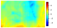
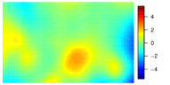
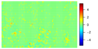
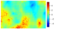
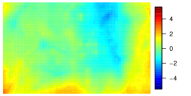
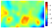
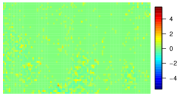
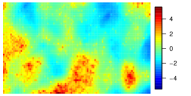
Figure 3: Calophyllum longifolium. The fixed covariate effects (without intercept), the weighted spatial component, the weighted error component, and the linear predictor (without intercept), using $U_{\sigma}=0.05$ (upper panels) and $U_{\sigma}=1.0$ (lower panels).

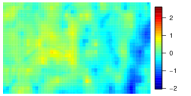
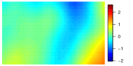
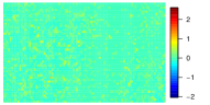
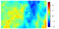
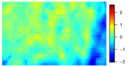
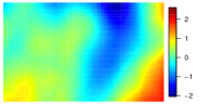
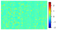
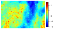
Figure 4: Oenocarpus mapoura: The fixed covariate effects (without intercept), the weighted spatial component, the weighted error component, and the linear predictor (without intercept), using $U_{\sigma}=0.05$ (upper panels) and $U_{\sigma}=1.0$ (lower panels).

Figures 3 and  4 illustrate the decomposition of the fitted log-intensity into three components – the fixed effects of covariates, the weighted spatially structured effect $\boldsymbol{u^{*}}\sqrt{\phi/\tau}$, the weighted error term $\boldsymbol{v}\sqrt{(1-\phi)/\tau}$ and the combination of these, the resulting linear predictor. Again, it is useful to consider the results for different scaling parameters, here $U_{\sigma}=0.05$ (upper panels) and $U_{\sigma}=1.0$ (lower panels). For both species, the summarised effect of the fixed covariates do not seem to change substantially with the different choices of the scaling parameters, while the spatially structured field clearly becomes more detailed. The error fields are also quite similar for both choices of $U_{\sigma}$.

The given results are robust to changes in the grid resolution of the study plot. This has been investigated dividing the given area into $50\times 100$ and $100\times 200$ grid cells, respectively. The difference in running time increasing from an average of 5 minutes to almost 2 hours when moving from the rougher to the finer resolution. By using a scaled spatial component in (2), we have ensured that both the results summarising the significance of covariates and the interpretations of the random field effects are similar when the grid cell resolution is changed. The PC prior for $\phi$ is by construction not invariant to grid resolution. However, Tables 1 and  2 illustrate that the estimates of $\phi$ are very similar using the two different grid resolutions. This can also be seen in Figure 5, which gives the posterior marginals of both $\sigma$ and $\phi$ when $U_{\sigma}=1$, for both resolutions.

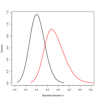
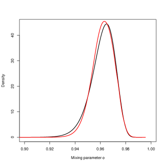
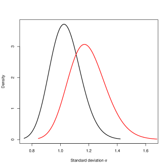
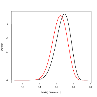
Figure 5: Posterior marginals for the standard deviation and the mixing parameter using grid resolution equal to $50\times 100$ and $100\times 200$ (red), when $U_{\sigma}=1.0$ for Calophyllum longifolium (upper panels) and Oenocarpus mapoura (lower panels).

3.4 A note on restricted spatial regression

A suggested alternative to the proposed method is to apply a restricted spatial regression approach, in which the spatial field is constrained to be orthogonal to the space spanned by the fixed covariates (Reich et al., 2006; Hodges and Reich, 2010; Hughes and Haran, 2013; Hanks et al., 2015). This is motivated by the fact that inclusion of spatially-correlated field in a model with fixed effects causes shrinkage and possibly biased estimates for the mean and variance of the fixed-effect coefficients (Reich et al., 2006; Hodges and Reich, 2010).

We can easily implement the idea of restricted spatial regression using (2). However, the implied assumption of no spatial confounding between the fixed and random effects is very strong as the observed fixed effects are attributed as much variability as possible. This typically leads to credible intervals that are inappropriately narrow under model misspecification (Hanks et al., 2015). We also notice that the obtained posterior means for the covariate effects are not extremely biased compared with the results obtained by GLM, except for the effect of Elevation for Oenocarpus mapoura, where it changes sign (Figure 2). Finally, using a restricted spatial regression approach we loose flexibility as the effects and credible intervals for the observed covariates are invariant to the choice of $U_{\sigma}$.

We can not recommend this approach, as it seems unrealistic to assume that unobserved biological processes reflected by the random fields are completely independent of the observed covariate information. In addition to false significances of the fixed covariates, interpretation of the resulting random fields is difficult. Meaningful interpretation of the posterior random fields is important as these can be viewed to reflect underlying biological processes and should not necessarily be considered as nuisance that needs to be accounted for (Hamel et al., 2012; Illian and Burslem, 2017). They may also be used for knowledge elicitation, pointing to biological mechanisms that cause aggregation but have not been included in the model, as we will see below.

4 Discussion and concluding remarks

For the species Calophyllum longifolium habitat association was expected based on its positive association with the slope habitat and negative association with the flat habitat in previous analyses of the same plot data (Harms et al., 2001). The species is known to be well dispersed, hence local clustering was not expected and the results have confirmed this (Harms et al., 2001; Muller-Landau et al., 2008). In addition, inspection of the spatial field in Figure 3 shows clear medium scale clustering that the covariates we examined cannot explain and may be related to the activity of the diverse assemblage of vertebrate secondary dispersers and seed predators that are known to be attracted to the fruits of this species (e.g. Adler and Kestell (1998)). Secondary dispersal and larder-hoarding of large tropical tree seeds may cause aggregations at medium scales that decouples the spatial structuring of recruitment from that of adults, which may be exacerbated by density-dependent mortality close to adult trees. These processes highlight the complexity of the interactions that determine spatial structure in tropical tree populations, including effects of biotic components of the community that are not captured by the covariates included in previous analyses. Through this example we have demonstrated that the modelling approach allows us to account for small and intermediate scale clustering while assessing the relative importance of either of these and also while providing potential interpretation of reason for larger scale clustering unexplained by the covariates.

For Oenocarpus mapoura significant habitat associations were expected (Harms et al., 2001; Muller-Landau et al., 2008) because this palm is a known specialist of the swamp habitat on the plot. The spatial field in Figure 4 shows a trend that covariates cannot explain, in particular, the high intensity of points in the bottom right hand corner of the plot. The cause of this cluster remains uncertain, but this corner has the lowest elevation across the plot and there may be aspects of the hydrological regime there that are particularly suitable for this species. In contrast to the other species, local clustering was to be expected here due to known seed dispersal limitation. This example allowed us to illustrate that we are able to establish the significance of covariate effects and their sensitivity to the smoothness (and hence potential overfitting) of the spatial field while accounting for both local and larger scale clustering and establishing their relative importance to the pattern.

An observed spatial point pattern represents one realisation of a random spatial point process. The fact that we have only one realisation of a random process is challenging as a statistical model including a spatially structured random field is easily overfitted to the observed pattern. This implies that valuable ecological information might not be revealed due to spatial confounding. However, underestimation of spatial autocorrelation could also give misleading results in terms of false significances of associations between the point pattern intensity of a species and covariates reflecting environmental conditions. For the given log-Gaussian Cox model, this trade-off is governed by the hyperprior choices for the precision of the included random field component. To avoid over-interpretation of the results, it is essential to fit models using a reasonable range of hyperprior choices.

In order to define reasonable hyperprior choices, the hyperparameters need to have clear interpretations. This is achieved here by viewing the spatially structured and unstructured random fields as one random component, parameterised in terms of two hyperparameters. The common precision parameter represents marginal precision and governs the total variability explained by the random component. The mixing parameter distributes this variability between the spatially structured and unstructured term. The given reparameterisation has a resemblance to modelling the nugget effect in geostatistics, which has been explained as a sum of a true “micro scale” nugget variance and variance due to measurement error (Cressie, 1993). By using the PC prior framework, we are able to control the effect and informativeness of these random fields using interpretable probability statements to tune the hyperpriors in an intuitive way. Also, the scaling of the spatially structured model ensures that given hyperprior choices can be transferred for analyses using different grid resolutions.

The given model formulation represents a first step towards explicitly communicating hyperprior choices in spatial point pattern analysis, fitting a log-Gaussian Cox process to an observed spatial point pattern. Ṫhe framework of log-Gaussian Cox processes is a versatile and flexible tool in spatial point pattern analysis, and care should be taken to facilitate correct ecological interpretation of the statistical results. The issues discussed here, are equally relevant in non-Bayesian settings where the choice of smoothing parameters impact the results in a similar way and an explicit discussion of these issues is equally ripe. An important future aim is to extend the given ideas to more complex modelling of the log-intensity, for example including non-linear effects of covariates, interaction between species and also to joint models of point patterns with marks as in Ho and Stoyan (2008) and Illian et al. (2012a). This requires further work in terms of model formulation, in which the total variance explained by random components is distributed between several model parameters, aiming to make the effect and influence of all hyperprior choices transparent.

5 Appendix: A brief review on computation of penalised complexity priors

The computation of PC priors for a given parameter $\xi$ is based on four principles. For ease of readability, these are listed below. We refer to Simpson et al. (2017) for further details on computation of PC priors, including a wide range of examples.

1. Occam’ razor:

Assume that $f_{1}=\pi(x\mid\xi)$ represents a flexible version of a simpler base model $f_{0}=\pi(x\mid\xi=\xi_{0})$. The prior for $\xi$ is computed to penalise deviation from the flexible model to the base model. This ensures that the constructed prior prefers the simpler model, until there is enough support for a more complex model.

2. Measure of complexity:

The PC prior is assigned to a function of the Kullback-Leibler divergence (KLD) (Kullback and Leibler, 1951), which represents a measure of complexity between two densities. Explicitly,

$$\mbox{KLD}(f_{1}\parallel f_{0})=\int f_{1}(x)\log\left(\frac{f_{1}(x)}{f_{0}(x)}\right)dx,$$

To facilitate interpretation, this deviation is transformed to a unidirectional measure of distance between the two densities, defined by

$$d(f_{1}\parallel f_{0})=\sqrt{2\mbox{KLD}(f_{1}\parallel f_{0})}.$$

3. Constant-rate penalisation:

The prior for $d$ is chosen according to a principle of constant rate penalisation

$$\frac{\pi(d+\delta)}{\pi(d)}=r^{\delta},\quad d,\delta\geq 0,$$

where $r\in(0,1)$. Consequently, the relative change in the prior for $d$ is independent of the actual distance and $d$ is exponentially distributed,

$$\pi(d)=\lambda\exp(-\lambda d),$$

where $r=\exp(\lambda)$. The prior for $\xi$ follows by a standard change of variable transformation and will always have its mode at the base model.

4. User-defined scaling:

The effect (or size of deviation from the base model) of a random component is adjusted by an intuitive scaling parameter, incorporating a user-defined probability statement for the parameter of interest. For example, this statement can be defined in terms of tail events, for example

$$P(Q(\xi)>U)=\alpha,$$

where $U$ represents an assumed upper limit for an interpretable transformation $Q(\xi)$, while $\alpha$ is a small probability, see on PC priors. This implies that the user should have an idea of a sensible size of the parameter (or any transformed variation) of interest.

References

- Adler and Kestell (1998) Adler, G. H. and Kestell, D. W. (1998). Fates of neotropical tree seeds influenced by spiny rats (proechimys semispinosus) 1. Biotropica, 30(4):677–681.
- Assunção and Krainski (2009) Assunção, R. and Krainski, E. (2009). Neighborhood dependence in Bayesian spatial models. Biometrical Journal, 5:851–869.
- Baddeley et al. (2015) Baddeley, A., Rubak, E., and Turner, R. (2015). Spatial Point Patterns: Methodology and Applications with R. Chapman and Hall/CRC Press, Boca Raton.
- Bagchi et al. (2011) Bagchi, R., Henrys, P. A., Brown, P. E., Burslem, D. F. R. P., Diggle, P. J., Gunatilleke, C. V. S., Gunatilleke, I. A. U. N., Kassim, A. R., Law, R., and Noor, S. (2011). Spatial patterns reveal negative density dependence and habitat associations in tropical trees. Ecology, 92(9):1723–1729.
- Banerjee et al. (2004) Banerjee, S., Carlin, B. P., and Gelfand, A. E. (2004). Hierarchical Modeling and Analysis for Spatial Data. Chapman and Hall/CRC Press, Boca Raton.
- Beguin et al. (2012) Beguin, J., Martino, S., Rue, H., and Cumming, S. G. (2012). Hierarchical analysis of spatially autocorrelated ecological data using integrated nested Laplace approximation. Methods in Ecology and Evolution, 3:921–929.
- Besag and Kooperberg (1995) Besag, J. and Kooperberg, C. (1995). On conditional and intrinsic autoregressions. Biometrika, 82:733–746.
- Besag et al. (1991) Besag, J., York, J., and Mollié, A. (1991). Bayesian image restoration, with two applications in spatial statistics. Annals of the Institute of Statistical Mathematics, 43:1–59.
- Brady and Weil (2013) Brady, N. C. and Weil, R. (2013). The Nature and Properties of Soils: Pearson New International Edition. Pearson Higher Ed.
- Chesson (2000) Chesson, P. (2000). Mechanisms of maintenance of species diversity. Annual Review of Ecology and Systematics, 31(1):343–366.
- Condit (1998) Condit, R. (1998). Tropical Forest Census Plots. Springer-Verlag and R. G. Landes Company, Berlin, Germany, and Georgetown, Texas.
- Condit et al. (2013) Condit, R., Engelbrecht, B. M., Pino, D., Pérez, R., and Turner, B. L. (2013). Species distributions in response to individual soil nutrients and seasonal drought across a community of tropical trees. Proceedings of the National Academy of Sciences, 110(13):5064–5068.
- Connell (1961) Connell, J. H. (1961). The influence of interspecific competition and other factors on the distribution of the barnacle chthamalus stellatus. Ecology, 42(4):710–723.
- Cressie (1993) Cressie, N. (1993). Statistics for Spatial Data. rev. ed. Wiley, New York.
- Diggle (2003) Diggle, P. J. (2003). Statistical analysis of spatial point patterns. 2nd edn. Arnold, London.
- Dornelas et al. (2006) Dornelas, M., Connolly, S. R., and Hughes, T. P. (2006). Coral reef diversity refutes the neutral theory of biodiversity. Nature, 440(7080):80–82.
- Hamel et al. (2012) Hamel, S., Yoccoz, N. G., and Baillard, J.-M. (2012). Statistical evaluation of parameters estimating autocorrelation and individual heterogeneity in longitudinal studies. Methods in Ecology and Evolution, 3:731–742.
- Hamill and Wright (1986) Hamill, D. N. and Wright, S. J. (1986). Testing the dispersion of juveniles relative to adults: a new analytic method. Ecology, pages 952–957.
- Hanks et al. (2015) Hanks, E. M., Schliep, E. M., Hooten, M. B., and Hoeting, J. A. (2015). Restricted spatial regression in practice: geostatistical models, confounding, and robustness under model misspecification. Environmetrics, 26:243–254.
- Harms et al. (2001) Harms, K. E., Condit, R., Hubbell, S. P., and Foster, R. B. (2001). Habitat associations of trees and shrubs in a 50-ha neotropical forest plot. Journal of Ecology, 89:947–959.
- Ho and Stoyan (2008) Ho, L. P. and Stoyan, D. (2008). Modelling marked point patterns by intensity-marked cox processes. Statistics & Probability Letters, 78(10):1194–1199.
- Hodges and Reich (2010) Hodges, J. S. and Reich, B. J. (2010). Adding spatially-correlated errors can mess up the fixed effect you love. The American Statistician, 64:325–334.
- Homburger et al. (2015) Homburger, H., Luscher, A., Scherer-Lorenzen, M., and Schneider, M. K. (2015). Patterns of livestock activity on heterogeneous subalpine pastures reveal distinct responses to spatial autocorrelation, environment and management. Movement Ecology, 3:35:1–15.
- Hubbell (2001) Hubbell, S. P. (2001). The Unified Neutral Theory of Biodiversity and Biogeography. Monographs in Population Biology 32, Princeton University Press.
- Hubbell et al. (2005) Hubbell, S. P., Condit, R., and Foster, R. B. (2005). Barro colorado forest census plot data.
- Hubbell et al. (1999) Hubbell, S. P., Foster, R. B., O’Brien, S. T., Harms, K. E., Condit, R., Wechsler, B., Wright, S. J., and de Lao, S. L. (1999). Light gap disturbances, recruitment limitation, and tree diversity in a neotropical forest. Science, 283:554–557.
- Hughes and Haran (2013) Hughes, J. and Haran, M. (2013). Dimension reduction and alleviation of confounding for spatial generalised linear mixed models. Journal of the Royal Statistical Society, Series B, 75:139–159.
- Illian and Burslem (2017) Illian, J. B. and Burslem, D. F. R. P. (2017). Improving the usability of spatial point processes methodology – an interdisciplinary dialogue between statistics and ecology. Advances in Statistical Analysis, to appear in.
- Illian et al. (2013) Illian, J. B., Martino, S., Sørbye, S. H., Gallego-Fernandez, J. B., Zunzunegui, M., Esquivias, M. P., and Travis, J. (2013). Fitting complex marked point patterns with integrated nested Laplace approximation (INLA). Methods in Ecology and Evolution, 4:305–315.
- Illian et al. (2008) Illian, J. B., Penttinen, A., Stoyan, H., and Stoyan, D. (2008). Statistical Analysis and Modelling of Spatial Point Patterns. Wiley, Chichester.
- Illian et al. (2012a) Illian, J. B., Sørbye, S. H., and Rue, H. (2012a). A toolbox for fitting complex spatial point process models using integrated nested Laplace approximation (INLA). Annals of Applied Statistics, 6:1499–1530.
- Illian et al. (2012b) Illian, J. B., Sørbye, S. H., Rue, H., and Hendrichsen, D. K. (2012b). Fitting a log Gaussian Cox process with temporally varying effects – a case study. Journal of Environmental Statistics, 3:1–29.
- John et al. (2007) John, R., Dalling, J. W., Harms, K. E., Yavitt, J. B., Stallard, R. F., Mirabello, M., Hubbell, S. P., Valencia, R., Navarrete, H., Vallejo, M., and Foster, R. B. (2007). Soil nutrients influence spatial distributions of tropical tree species. Proceeding of the National Academy of Science of the United States of America, 104:864–869.
- Kang et al. (2015) Kang, S. Y., McGree, J., Baade, P., and Mengersen, K. (2015). A case-study for modelling cancer incidence using bayesian spatio-temporal models. Australian and New Zealand Journal of Statistics, 57:325–245.
- Kang et al. (2014) Kang, S. Y., McGree, J., and Mengersen, K. (2014). The choice of spatial scales and spatial smoothness priors for various spatial patterns. Spatial and Spatio-temporal Epidemiology, 10:11–26.
- Klein and Kneib (2016) Klein, N. and Kneib, T. (2016). Scale-dependent priors for variance parameters in structured additive distributional regression. Bayesian Analysis, 11(4):1071–1106.
- Kullback and Leibler (1951) Kullback, S. and Leibler, R. A. (1951). On information and sufficiency. The Annals of Mathematical Statistics, pages 79–86.
- Law et al. (2009) Law, R., Illian, J., Burslem, D. F., Gratzer, G., Gunatilleke, C., and Gunatilleke, I. (2009). Ecological information from spatial patterns of plants: insights from point process theory. Journal of Ecology, 97(4):616–628.
- Lindgren et al. (2011) Lindgren, F., Rue, H., and Lindström, J. (2011). An explicit link between Gaussian fields and Gaussian Markov random fields: the stochastic partial differential equation approach. Journal of the Royal Statistical Society, Ser. B, 73:423–498.
- Lunn et al. (2009) Lunn, D., Spiegelhalter, D., Thomas, A., and Best, N. (2009). The BUGS project: Evolution, critique and future directions. Statistics in Medicine, 28:3049–3067.
- Møller et al. (1998) Møller, J., Syversveen, A. R., and Waagepetersen, R. P. (1998). Log Gaussian Cox processes. Scandinavian Journal of Statistics, 25:451–482.
- Møller and Waagepetersen (2007) Møller, J. and Waagepetersen, R. P. (2007). Modern statistics for spatial point processes (with discussion). Scandinavian Journal of Statistics, 34:643–711.
- Muller-Landau et al. (2008) Muller-Landau, H. C., Wright, S. J., Calderón, O., Condit, R., and Hubbell, S. P. (2008). Interspecific variation in primary seed dispersal in a tropical forest. Journal of Ecology, 96(4):653–667.
- Papoila et al. (2014) Papoila, A. L., Riebler, A., Amaral-Turkman, A., Sao-Joao, R., Ribeiro, C., Geraldes, C., and Miranda, A. (2014). Stomach cancer incidence in southern portugal 1998-2006: A spatio-temporal analysis. Biometrical Journal, 56:403–415.
- Reich et al. (2006) Reich, B. J., Hodges, J. S., and Zadnik, V. (2006). Effects of residual smoothing on the posterior of the fixed effects in disease-mapping models. Biometrics, 62:1197–1206.
- Riebler et al. (2016) Riebler, A., Sørbye, S. H., Simpson, D., and Rue, H. (2016). An intuitive Bayesian spatial model for disease mapping that accounts for scaling. Statistical Methods in Medical Research, 25:1145–1165.
- Roos and Held (2011) Roos, M. and Held, L. (2011). Sensitivity analysis in Bayesian generalized linear mixed models for binary data. Bayesian Analysis, 6:259–278.
- Rue and Held (2005) Rue, H. and Held, L. (2005). Gaussian Markov Random Fields. Chapman & Hall/CRC, Boca Raton.
- Rue et al. (2009) Rue, H., Martino, S., and Chopin, N. (2009). Approximate Bayesian inference for latent Gaussian models by using integrated nested Laplace approximations (with discussion). Journal of the Royal Statistical Society, Ser. B, 71:319–392.
- Schreeg et al. (2010) Schreeg, L. A., Kress, W. J., Erickson, D. L., and Swenson, N. G. (2010). Phylogenetic analysis of local-scale tree soil associations in a lowland moist tropical forest. PLoS ONE, 5:1–10.
- Shen et al. (2013) Shen, G., He, F., Waagepetersen, R., Sun, I., Hao, Z., Chen, Z.-S., Yu, M., et al. (2013). Quantifying effects of habitat heterogeneity and other clustering processes on spatial distributions of tree species. Ecology, 94(11):2436–2443.
- Simpson et al. (2016) Simpson, D., Illian, J., Lindgren, F., Sørbye, S. H., and Rue, H. (2016). Going off grid: computationally efficient inference for log-Gaussian Cox processes. Biometrika, 103:49–70.
- Simpson et al. (2017) Simpson, D., Rue, H., Riebler, A., Martins, T. G., and Sørbye, S. H. (2017). Penalising model component complexity: A principled, practical approach to constructing priors. Statistical Science, 32:1–28.
- Sørbye and Rue (2014) Sørbye, S. H. and Rue, H. (2014). Scaling intrinsic Gaussian Markov random field priors in spatial modelling. Spatial Statistics, 8:39–51.
- Spiegelhalter et al. (2002) Spiegelhalter, D. J., Best, N. G., Carlin, B. P., and der Linde A, A. V. (2002). Bayesian measures of model complexity and fit (with discussion). Journal of the Royal Statistical Society, Series B, 64:583–616.
- Velázquez et al. (2016) Velázquez, E., Martínez, I., Getzin, S., Moloney, K. A., and Wiegand, T. (2016). An evaluation of the state of spatial point pattern analysis in ecology. Ecography, 39:1042–1055.
- Waagepetersen et al. (2016) Waagepetersen, R., Guan, Y., Jalilian, A., and Mateu, J. (2016). Analysis of multispecies point patterns by using multivariate log-gaussian cox processes. Journal of the Royal Statistical Society, Series C, 65:77–96.
- Wiegand and Moloney (2014) Wiegand, T. and Moloney, K. A. (2014). Handbook of Spatial Point-Pattern Analysis in Ecology. Chapman and Hall/CRC Press, Boca Raton.