How to Differentiate Collective Variables in Free Energy Codes: Computer-Algebra Code Generation and Automatic Differentiation

Abstract

The proper choice of collective variables (CVs) is central to biased-sampling free energy reconstruction methods in molecular dynamics simulations. The PLUMED 2 library, for instance, provides several sophisticated CV choices, implemented in a C++ framework; however, developing new CVs is still time consuming due to the need to provide code for the analytical derivatives of all functions with respect to atomic coordinates. We present two solutions to this problem, namely (a) symbolic differentiation and code generation, and (b) automatic code differentiation, in both cases leveraging open-source libraries (SymPy and Stan Math respectively). The two approaches are demonstrated and discussed in detail implementing a realistic example CV, the local radius of curvature of a polymer. Users may use the code as a template to streamline the implementation of their own CVs using high-level constructs and automatic gradient computation.

PROGRAM SUMMARY

Program Title:
Practical approaches to the differentiation of collective variables in free energy codes: computer-algebra code generation and automatic differentiation
Licensing provisions:
GNU Lesser General Public License Version 3 (LGPL-3)
Programming languages:
C++, Python
Nature of problem:
The C++ implementation of collective variables (CVs, functions of atomic coordinates to be used in biased sampling applications) in biasing libraries for atomistic simulations, such as PLUMED [1], requires computation of both the variable and its gradient with respect to the atomic coordinates; coding and testing the analytical derivatives complicates the implementation of new CVs.
Solution method:
The paper shows two approaches to automate the computation of CV gradients, namely, symbolic differentiation with code generation and automatic code differentiation, demonstrating their implementation entirely with open-source software (respectively, SymPy and the Stan Math Library).
Additional comments:
The paper’s accompanying code serves as an example and template for the methods described in the paper; it is distributed as the two modules curvature_codegen and curvature_autodiff integrated in PLUMED 2’s source tree; the latest version is available at https://github.com/tonigi/plumed2-automatic-gradients .

1 Introduction

Biased approaches to molecular dynamics (MD) enable the sampling of events whose occurrence would otherwise be prohibitively rare on the time scales affordable by direct (unbiased) integration of the equations of motion. Central to the possibility to obtain converged estimates of thermodynamic quantities is the search of appropriate projections of the system state [1]; in turn, this enables the search of a reaction coordinate to effectively push the specific system out of free energy minima. When an appropriate reaction coordinate is selected, the sampling of a system can be accelerated through a number of biased sampling methods, such as umbrella sampling [2], metadynamics [3], SuMD [4] and others [5], most of which enable the reconstruction of the free energy landscape, and in some cases the kinetics [6, 7], on the space spanned by the chosen variables. The availability of a wide range of functions of atomic coordinates (collective variables or CVs) is thus a valuable asset in the construction of proper reaction coordinates [8].

PLUMED 2 is a widely-used engine to perform biased sampling simulations in atomistic simulations [9]. Part of PLUMED’s success is due to the number and variety of collective variables implemented (see e.g. [10, 11, 12]), enabling projections of the system state on “axes” of intuitive value, and the number of CVs implemented in PLUMED 2 has been growing steadily (Figure 1). Users can incorporate their own CVs coding them in C++; however, the implementation of complex functions is complicated by the need to compute gradients with respect to atomic coordinates, which increases the complexity and debugging time of the corresponding source codes.

Here, we present two approaches to automatically implement CV gradients:

1. a symbolic differentiation with code generation approach, where the SymPy computer algebra system (CAS) [13] is used to derive the expressions and automatically produce an equivalent C function (Section 2); and

2. an automatic code differentiation approach, using the reverse-mode code differentiation capabilities provided by the Stan Math library [14] (Section 3).

We demonstrate the two approaches on the simple (yet non trivial) case of a CV computing the local curvature of a polymer, approximated as the radius of curvature of a circle passing through three consecutive atoms. The two approaches provide identical numerical results and are based on mature and well-known open source libraries. Their different characteristics will be presented in the discussion section.

Example code is made available as open-source respectively in PLUMED 2’s curvature_codegen and curvature_autodiff modules; from there, the corresponding source files can be used as templates for the implementation of customized CVs.

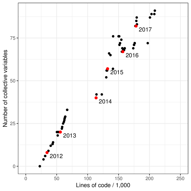
Figure 1: Growth of the number of CVs in PLUMED 2 and the corresponding code base (lines of C++ code in the master branch, including headers and inline documentation; the count also includes support functions, command line utilities and file readers).

1.1 Background

A CV is a function of a system’s state through the coordinates of its $n$ particles, namely: [15]

$$f(\mathbf{x})=f(\mathbf{x}_{1},\ldots,\mathbf{x}_{n})$$

Applying biases to CVs implies that the system is subject to a potential $V$ which depends on the coordinates solely through $f$:

$$V(\mathbf{x})=V_{1}(f(\mathbf{x}))$$

The bias potential translates to forces acting on each atom, which are computed in the biasing library and passed to the molecular dynamics (MD) engine. The MD code adds them to those due to the force field, and integrates the equations of motion. From the chain differentiation rule,

$$\mathbf{F}(\mathbf{x})=-\nabla_{\mathbf{x}}V_{1}(f(\mathbf{x}))=-\frac{\partial V_{1}(f)}{\partial f}\nabla_{\mathbf{x}}f(\mathbf{x})$$

here $\partial V_{1}/\partial f$ is the generalized force, set by the chosen biasing scheme (e.g., a time-dependent sum of Gaussians in the case of metadynamics), while $\nabla_{\mathbf{x}}f$ depends only on the functional form of $f$ and the system state $\mathbf{x}$. Implementation of a CV requires the programmer to write code for $f(\mathbf{x})$ and its derivatives with respect to all of the arguments (number of involved atoms times three Cartesian components).

1.2 Radius of curvature

To illustrate the methods, we shall use as an example the radius of curvature at a given atom along a polymer. A natural choice for this quantity is to compute the radius $R$ of the circle (circumcircle) passing through three given points $\mathbf{r}_{1},\mathbf{r}_{2}$ and $\mathbf{r}_{3}$ (Figure 2), e.g. the centers of consecutive C$\alpha$ atoms. The diameter $2R$ is obtained elementarily via the sine rule as the ratio between a side of the triangle formed by the points and the sine of the opposing angle, i.e., calling $\mathbf{r}_{ij}=\mathbf{r}_{i}-\mathbf{r}_{j}$ and $\theta_{123}$ the angle at $\mathbf{r}_{2}$,

$$2R=\frac{|\mathbf{r}_{13}|}{\sin\theta_{123}}\qquad\mbox{with}\qquad\cos\theta_{123}=\frac{\mathbf{r}_{12}\cdot\mathbf{r}_{23}}{|\mathbf{r}_{12}||\mathbf{r}_{23}|}$$ (1)

The above expression is compact in vector notation, but the expressions for its gradient in Cartesian coordinates, i.e. the components of $\nabla_{\mathbf{x}}R(\mathbf{r}_{1},\mathbf{r}_{2},\mathbf{r}_{3})$ with $\mathbf{x}=(r_{1x},r_{1y},\ldots,r_{3z})$, are unwieldy (see the notebook CurvatureCodegen.ipynb).

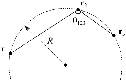
Figure 2: The radius of curvature as a collective variable $R(\mathbf{r}_{1},\mathbf{r}_{2},\mathbf{r}_{3})$.

1.3 Edge cases and inverse radius

Computer-assisted code generation does not automatically guarantee that the functions are well-defined in all conditions. Of special relevance are singularities on edge cases, such as collinearity ($R\to\infty$) in the curvature example. Edge cases are generally set aside when deriving expressions “on paper”, but their occurrence in computer code, however rare, must be caught to avoid crashes in simulations.

In the example of this paper the user-visible INVERSE flag is added to the curvature collective variables in order to illustrate a possible approach to removing singularities, and to show how CV computations can be made to depend on user-defined parameter. The idea is that the reciprocal of the radius is a better-behaved collective variable, lacking the singularity (infinite radius) for the case of three collinear points (which may arise e.g. when the initial configuration of a polymer is generated artificially). Of note, this solution does not eliminate a singularity in the gradient, whose limit for collinear atoms is still undefined.

2 Generating code with a computer algebra system

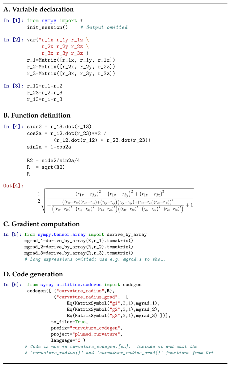
Figure 3: Symbolic differentiation with code generation approach – A SymPy Jupyter notebook generating C code for the collective variable R and its gradient. (See also the calling code in the module curvature_codegen/Curvature.cpp, and the notebook CurvatureCodegen.ipynb containing the extended version of this figure.)

CAS manipulate mathematical expressions in symbolic form. They usually build internal representations of expression as trees, which are subject to transformations encoding algebraic manipulations (such as differentiation) as pattern-matching rules. When desired, the trees can be evaluated numerically, printed, or transformed in other languages. It is therefore tempting to use CAS to generate lengthy mathematical expressions for later compilation and inclusion in CV code.

We used the SymPy package [13] to implement the collective variable as a mathematical expression, compute its gradient symbolically, and convert the function and the gradient into C code for inclusion in PLUMED. SymPy turned out to be suitable for this task because of three reasons: it is open source and freely available; it provides excellent symbolic manipulation and simplification features (among others); and generates stand-alone C code which does not rely on external libraries. It has been used for code-generation purposes in other contexts [16].

Figure 3 shows the steps required for this approach, i.e.:

1. Atom coordinates are introduced as SymPy symbols.

2. The collective variable is defined following eq. (1); note the use of vector algebra.

3. Symbolic computation of $\nabla_{\mathbf{x}}R(\mathbf{r}_{1},\mathbf{r}_{2},\mathbf{r}_{3})$.

4. Code generation is performed with the codegen() function, which translates R and mgrad in the files curvature_codegen.[ch].

The code generated is included via a wrapper, which makes the functions curvature_radius and curvature_radius_grad available for use in the Curvature class. The rest of the code does not depend on the specific CV function, and can be reused from the example’s source (Curvature.cpp), available in PLUMED’s curvature_codegen module. The module also contains a multicolvar implementation, enabling the use of aggregated curvature radius values along a polymer (e.g., its mean, minimum and so on).

An extended version of the notebook of Figure 3 distributed with the source code also demonstrates how substitution operators were used within the CAS to check the results of the derivations with respect to known values and limits towards edge cases (in this case, collinear points). There was no need to generate separate expressions for the inverse radius, whose gradient is trivially implemented in C++ via the chain rule.

Finally, depending on the symmetry of the CV and the number of atoms involved, it may be more natural to differentiate with respect to atoms’ distance vectors rather than coordinates, and then apply the chain rule in the calling code. The code generation steps proceed straightforwardly as above (final examples in the notebook).

2.1 Symbolic Common Subexpression Elimination

Inspection of the code generated by the “naive” CAS approach in Figure 3 shows repeatedly-computed expressions that could be made more efficient with the introduction of intermediate variables. This is due to the fact that the translation of a formula derived by contemporary CAS systems into code form usually happens all at once on the basis of the explicit expression, which may be unnecessarily (or even intractably) complex; in particular, the translation does not re-use the subexpressions which are generated during differentiation. As an example, consider the derivative $\frac{d}{dx}\exp(\exp(f(x))=\exp(\exp(f(x)))\exp(f(x))f^{\prime}(x)$: even though the $\exp(f(x))$ subexpression could in principle be evaluated just once, this simplification can not be rendered in the mathematical formula.

SymPy can indeed exploit opportunities for common subexpression elimination (CSE) at a symbolic level, as demonstrated in the section Common subexpression elimination of the notebook. The source code of the gradient function generated by codegen() contains approximately 1,980 floating-point (FP) operators. The symbolic CSE step, in contrast, produces the source code of an equivalent gradient function containing just 101 FP operators (the radius function has 44).

It is important to note that most of the redundant arithmetic operations are optimized by the compiler anyway, because CSE is a standard pass in current compiler optimizations; however, the extent of subexpressions that are going to be recognized at this low-level pass is hard to assess a priori. In Section 4 we report actual FP counts measured on naive and CSE code downstream of the compiler optimization passes.

3 Automatic code differentiation

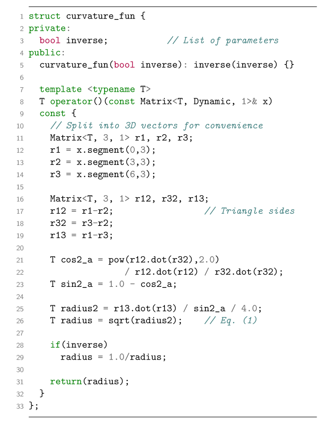
Figure 4: Automatic code differentiation approach – Automatically differentiable code implementing the radius of curvature CV. The “abstract” type T is used for variables and parameters. The use of Eigen types allows writing Eq. (1) in a compact vector form close to the textbook one. See CurvatureAutoDiff.cpp in the PLUMED module curvature_autodiff for full code.

A different and independent approach to gradient computation is through automatic code differentiation, a powerful method which calculates gradients of functions defined by (in principle) arbitrary algorithms. In short, the gradient computation “mirrors” each elementary step executed by the function being derived by keeping track of the partial derivatives (“adjunct”) of each variable, propagating them via the chain rule; the components of a gradient are computed together in a single pass. It has the same computational complexity as the original code and hence, for example, loops of arbitrary length can be differentiated even when the number of iterations is only known at run time (see [14] for a thorough explanation).

We rely on Stan Math, a header-only library part of the Stan probabilistic programming language, to provide reverse-mode automatic differentiation for C++ code [17, 14]. The library uses template-based metaprogramming, meaning that expressions can be written with the same semantics used for common floating-point operations, while in reality operator overloading is used to construct the code and data structures necessary for differentiation.

In practice, a convenient way to introduce this in PLUMED is to wrap the function to be differentiated in a C++ functor, as shown in Figure 4. Apart from boilerplate semantics, the body of function can be written as customary, with the following assumptions:

• arguments are passed as one single-column Matrix object (typically as long as the number of atomic coordinates involved in the collective variable);

• arguments and return value should all be of “type” T;

• parameters, if needed, can passed through the functor constructor (see section 3.2 for details).

The gradient computation is transparent for the programmer. The collective variable’s compute() method, invoked by PLUMED at each time step of the simulation, will call stan::math::gradient(), perform any vector reshaping necessary, then set the derivatives to inform the rest of the code of the bias forces to be applied. The compute method is thus largely independent on the CV at hand, and can be re-used unchanged from the complete example provided in the CurvatureAutoDiff.cpp file.

3.1 Linear algebra and special functions

The example code expresses the curvature function concisely by using dot() inner product operators; they operate between two $3\times 1$ vectors (the sides of the triangle), declared of type Eigen::Matrix<T,1,3>. Eigen, a template-based linear algebra library, defines operations on dense and sparse vectors and matrices, and is part of Stan Math. Its scope is in fact much larger, providing e.g. determinants, eigenvectors and many decomposition types [18].

In addition to the code differentiation features, the Stan Math library provides a remarkable range of special functions and distributions, whose enumeration is beyond the scope of this paper. Functions can also be defined through differential equations and differentiated with respect to their parameters, thanks to SUNDIALS’ CVodes library [14, 17, 19].

3.2 Dealing with parameters

Functors expect only an N-dimensional vector of variables; lines 3–5 of Figure 4 show how additional parameters (e.g. set by the user in PLUMED’s input file) can be passed to the functor constructor.

Note that parameters should not be passed via the arguments (e.g., as variables in addition to the atom coordinates) because, besides restricting their types to floating point numbers, the function would be unnecessarily differentiated with respect to them (although reverse mode differentiation is relatively efficient in this regard).

4 Performance considerations

In order to estimate real-world performance, i.e. downstream of optimizations performed automatically by modern compilers, we compared the optimized executables in terms of FP instructions actually executed by the CPU. Measurements were obtained through hardware FP counters, namely FP_COMP_OPS_EXE:SSE_SCALAR_DOUBLE and vector analogs. Table 1 reports the performance of the functions performing the radius and gradient computations, in terms of number of double-precision FP instructions, and CPU time required per calculation (medians and inter-quartile ranges over 10 runs of $10^{7}$ evaluations each).

In Section 2.1 we reported that the number of FP operators found in the naive and symbolic CSE-generated source codes differed by a factor of 20. The dramatic difference is not reflected in the compiled code, indicating that the compiler optimized out almost all of the redundant expressions. The high-level CSE step was still beneficial, reducing the final FP instruction count by further 45 (out of 137).

Interestingly, the automatic differentiation approach used roughly the same number of floating-point operations as the CAS-generated code. Its actual run time was longer, likely due to non-FP operations such as method calls, expected because of the use of objects representing variables along with their adjoints. Note also that run times varied widely with “fast-math”-like optimizations, and that hardware counters may be affected by approximations [20].

Finally, we remark that all of the above measurements included the FP-intensive part of the calculations only. If speed is a concern, the overhead at the interface with the free-energy code (e.g., reshaping coordinate arrays) should be accounted, as it may dwarf the cost of the functions proper.

Floating-point ops. CPU time (ns) Method $R$ and $\nabla R$ $\nabla R$ only $R$ and $\nabla R$ $\nabla R$ only Code generation 173 137 $125.98\pm 0.07$ $110.36\pm 0.02$ Code generation, symbolic CSE 128 92 $60.19\pm 0.01$ $48.48\pm 0.11$ Automatic differentiation 148 — $532.61\pm 7.82$ —

Table 1: Number of floating-point operations and CPU time required by one evaluation of the gradient of the curvature function with the approaches presented in the paper. One iteration of either the curvature function and its gradient, or gradient only, as indicated in the column headers, is measured; time spent in the interface with the free energy code is not included. (Medians and inter-quartile ranges over $10\times 10^{7}$ calls; Intel Xeon CPU E5-2697 v4 at 2.30GHz, GCC version 6.1.0, optimization O3.)

5 Discussion

The two approaches discussed yield, as expected, numerical results equal within machine precision. Which of the two is preferred depends on the complexity of the specific problem being addressed.

On the one hand, symbolic differentiation may be closer to the “classroom” approach, where a closed form expression is derived top-down. CAS assist the development of the final formulas, e.g. enabling complex substitutions, differentiations, and simplifications. Symbols can also be replaced by values and evaluated at any time necessary, which is generally useful for quickly checking the consistency of equations with known results. Also, structuring computations as “notebook” format, while optional, is an approach favoured by most CAS as a means to keep a readable and reproducible record of the steps leading to a particular formula or code [21].

The most important limitation of CAS code generators is that they do not handle generic functions defined as algorithms (e.g., loops until convergence). As discussed above, the automatic code differentiation approach largely solves the issue: it is therefore expected to be the preferred way to implement very complex CVs in real-world problems. The vastly increased generality comes at some expense of convenience, for the edit-compile-run cycle is somewhat at odds with notebook-style readability and the interactive testing it affords. Performance-wise, the approaches are very close in terms of amount of the floating-point calculations required; and at least in the same order of magnitude in terms of CPU time.

An even more high-level language approach than the ones presented here would be to evaluate mathematical functions in an embedded Python interpreter, an approach recently implemented in PLUMED (also used in [22]). This may be desirable for casual coding, but likely inefficient, as the critical portion of the calculations would happen in an interpreted language.

The code templates presented have been tested in combination with software version widely in use at the time of writing (Table 2). The libraries are under active development, so code may require minor adaptations with future releases. Regression testing and continuous integration of the PLUMED code base ensure that incompatibilities, should they arise, will be spotted timely.

Software	Version
Plumed	2.4.0
Python (Anaconda)	3.6.4
SymPy	1.0
Stan Math library	2.16.0
GCC	6.1.0
Clang++	3.8.1
Intel ICC	18.0.1

Table 2: Software versions tested.

6 Conclusion

This paper presented two methods intended to substantially reduce the barrier to the development of functions of atomic coordinates. While the resulting code may not as optimized as hand-written one, it is hoped that the approaches presented will enable the extension of free energy codes with further CVs, significant from the points of view of structural biology, biological relevance, or closeness to experimental observables, whose complexity would have otherwise made their implementation prohibitive.

7 Acknowledgements

I would like to thank Prof. G. Bussi and Prof. C. Camilloni for discussions on the applications of automatic differentiation and comments on the manuscript. I acknowledge CINECA awards under the ISCRA initiative for the availability of high performance computing resources and support. Research funding from Acellera Ltd. is gratefully acknowledged.

8 References

References

- [1] Tribello GA, Bonomi M, Branduardi D, Camilloni C, Bussi G. PLUMED 2: New feathers for an old bird. Computer Physics Communications. 2014 Feb;185(2):604-13.

References

- [1] A. Laio, F. L. Gervasio, Metadynamics: a method to simulate rare events and reconstruct the free energy in biophysics, chemistry and material science, Reports on Progress in Physics 71 (12) (2008) 126601. doi:10.1088/0034-4885/71/12/126601.
- [2] G. M. Torrie, J. P. Valleau, Nonphysical sampling distributions in Monte Carlo free-energy estimation: Umbrella sampling, Journal of Computational Physics 23 (2) (1977) 187–199. doi:10.1016/0021-9991(77)90121-8.
- [3] A. Laio, M. Parrinello, Escaping free-energy minima, Proceedings of the National Academy of Sciences of the United States of America 99 (20) (2002) 12562–12566. doi:10.1073/pnas.202427399.
- [4] V. Salmaso, M. Sturlese, A. Cuzzolin, S. Moro, Exploring Protein-Peptide Recognition Pathways Using a Supervised Molecular Dynamics Approach, Structure 25 (4) (2017) 655–662.e2. doi:10.1016/j.str.2017.02.009.
- [5] D. Hamelberg, J. Mongan, J. A. McCammon, Accelerated molecular dynamics: A promising and efficient simulation method for biomolecules, The Journal of Chemical Physics 120 (24) (2004) 11919–11929. doi:10.1063/1.1755656.
- [6] L. Mollica, S. Decherchi, S. R. Zia, R. Gaspari, A. Cavalli, W. Rocchia, Kinetics of protein-ligand unbinding via smoothed potential molecular dynamics simulations, Scientific Reports 5 (2015) srep11539. doi:10.1038/srep11539.
- [7] H. Sun, Y. Li, M. Shen, D. Li, Y. Kang, T. Hou, Characterizing Drug–Target Residence Time with Metadynamics: How To Achieve Dissociation Rate Efficiently without Losing Accuracy against Time-Consuming Approaches, Journal of Chemical Information and Modelingdoi:10.1021/acs.jcim.7b00075.
- [8] T. Giorgino, A. Laio, A. Rodriguez, METAGUI 3: A graphical user interface for choosing the collective variables in molecular dynamics simulations, Computer Physics Communications 217 (2017) 204–209. doi:10.1016/j.cpc.2017.04.009.
- [9] G. A. Tribello, M. Bonomi, D. Branduardi, C. Camilloni, G. Bussi, Plumed 2: New feathers for an old bird, Computer Physics Communications 185 (2) (2014) 604–613. doi:10.1016/j.cpc.2013.09.018.
- [10] G. A. Tribello, F. Giberti, G. C. Sosso, M. Salvalaglio, M. Parrinello, Analyzing and Driving Cluster Formation in Atomistic Simulations, Journal of Chemical Theory and Computation 13 (3) (2017) 1317–1327. doi:10.1021/acs.jctc.6b01073.
- [11] D. Branduardi, F. L. Gervasio, M. Parrinello, From A to B in free energy space, The Journal of Chemical Physics 126 (5) (2007) 054103. doi:10.1063/1.2432340.
- [12] M. Bonomi, C. Camilloni, Integrative structural and dynamical biology with PLUMED-ISDB, Bioinformatics 33 (24) (2017) 3999–4000. doi:10.1093/bioinformatics/btx529.
- [13] A. Meurer, C. P. Smith, M. Paprocki, O. Čertík, S. B. Kirpichev, M. Rocklin, A. Kumar, S. Ivanov, J. K. Moore, S. Singh, T. Rathnayake, S. Vig, B. E. Granger, R. P. Muller, F. Bonazzi, H. Gupta, S. Vats, F. Johansson, F. Pedregosa, M. J. Curry, A. R. Terrel, S. Roučka, A. Saboo, I. Fernando, S. Kulal, R. Cimrman, A. Scopatz, SymPy: symbolic computing in Python, PeerJ Computer Science 3 (2017) e103. doi:10.7717/peerj-cs.103.
- [14] B. Carpenter, M. D. Hoffman, M. Brubaker, D. Lee, P. Li, M. Betancourt, The Stan Math Library: Reverse-Mode Automatic Differentiation in C++, arXiv:1509.07164 [cs]ArXiv: 1509.07164.
- [15] G. Fiorin, M. L. Klein, J. Hénin, Using collective variables to drive molecular dynamics simulations, Molecular Physics 111 (22-23) (2013) 3345–3362. doi:10.1080/00268976.2013.813594.
- [16] A. Mushtaq, K. Olaussen, Automatic code generator for higher order integrators, Computer Physics Communications 185 (5) (2014) 1461–1472. doi:10.1016/j.cpc.2014.01.012.
- [17] B. Carpenter, A. Gelman, M. Hoffman, D. Lee, B. Goodrich, M. Betancourt, M. Brubaker, J. Guo, P. Li, A. Riddell, Stan: A probabilistic programming language, Journal of Statistical Software, Articles 76 (1) (2017) 1–32. doi:10.18637/jss.v076.i01.
- [18] G. Guennebaud, B. Jacob, et al., Eigen v3, http://eigen.tuxfamily.org (2010).
- [19] A. C. Hindmarsh, P. N. Brown, K. E. Grant, S. L. Lee, R. Serban, D. E. Shumaker, C. S. Woodward, SUNDIALS: Suite of Nonlinear and Differential/Algebraic Equation Solvers, ACM Trans. Math. Softw. 31 (3) (2005) 363–396. doi:10.1145/1089014.1089020.
- [20] V. M. Weaver, D. Terpstra, S. Moore, Non-determinism and overcount on modern hardware performance counter implementations, in: 2013 IEEE International Symposium on Performance Analysis of Systems and Software (ISPASS), 2013, pp. 215–224. doi:10.1109/ISPASS.2013.6557172.
- [21] F. Perez, B. E. Granger, IPython: A System for Interactive Scientific Computing, Computing in Science Engineering 9 (3) (2007) 21–29. doi:10.1109/MCSE.2007.53.
- [22] R. Galvelis, Y. Sugita, Neural Network and Nearest Neighbor Algorithms for Enhancing Sampling of Molecular Dynamics, Journal of Chemical Theory and Computation 13 (6) (2017) 2489–2500. doi:10.1021/acs.jctc.7b00188.