Deconvolving the Wedge: Maximum-Likelihood Power Spectra via Spherical-Wave Visibility Modeling

Abstract

Direct detection of the Epoch of Reionization (EoR) via the red-shifted 21-cm line will have unprecedented implications on the study of structure formation in the infant Universe. To fulfill this promise, current and future 21-cm experiments need to detect this weak EoR signal in the presence of foregrounds that are several orders of magnitude larger. This requires extreme noise control and improved wide-field high dynamic-range imaging techniques. We propose a new imaging method based on a maximum likelihood framework which solves for the interferometric equation directly on the sphere, or equivalently in the $uvw$-domain. The method uses the one-to-one relation between spherical waves and spherical harmonics (SpH). It consistently handles signals from the entire sky, and does not require a $w$-term correction. The spherical-harmonics coefficients represent the sky-brightness distribution and the visibilities in the $uvw$-domain, and provide a direct estimate of the spatial power spectrum. Using these spectrally-smooth SpH coefficients, bright foregrounds can be removed from the signal, including their side-lobe noise, which is one of the limiting factors in high dynamics range wide-field imaging. Chromatic effects causing the so-called “wedge" are effectively eliminated (i.e. deconvolved) in the cylindrical ($k_{\perp},k_{\parallel}$) power spectrum, compared to a power spectrum computed directly from the images of the foreground visibilities where the wedge is clearly present. We illustrate our method using simulated LOFAR observations, finding an excellent reconstruction of the input EoR signal with minimal bias.

1 Introduction

The Epoch of Reionization (EoR) is an important milestone in tracing back the whole history of the Universe. At this epoch the first luminous sources largely influence the conditions of the intergalactic medium and therefore played a significant role in galaxy formation and its evolution. New discoveries of sources at high redshift (z $\sim$ 8) have pinned down the bright end of the galaxy luminosity function (Bouwens et al., 2010; Oesch et al., 2013). In parallel, a number of indirect techniques came up with tight constraints for the redshift of the ionized to neutral phase transition through cosmic microwave background (CMB) which tries to constraint reionization from the optical depth of Thomson scattering to the CMB (Planck Collaboration et al., 2014), but the redshift range of the EoR is significantly less certain. The tail of reionization is also well probed by Gunn-Peterson absorption troughs in the spectra of high redshift quasars (for a detailed review see Fan et al. (2006)), Ly$\alpha$ emitting galaxies (Schenker et al., 2013; Treu et al., 2013) and the Ly-$\alpha$ absorption profile toward very distant quasars (Bolton et al., 2011; Bosman & Becker, 2015). Although, at higher redshifts ($z\geq 6$) the interpretation of the Lyman-$\alpha$ quasar absorption data becomes more uncertain. We note that a new population of galaxies discovered by the various probes still fall well short of reionizing the universe consistently with the inferred redshifts of the CMB optical depth measurements (Robertson et al., 2013; Robertson et al., 2015). In addition to these probes, the statistical technique targeting the 21-cm spin flip transition of neutral hydrogen at high redshifts has been well recognized as a unique probe of the EoR (Wyithe & Loeb, 2004; Bharadwaj & Ali, 2005; Furlanetto et al., 2006; Mesinger, 2010; Morales & Wyithe, 2010; Mellema et al., 2013) which can reveal the large-scale fluctuations in the ionization state and temperature of the IGM, and open up an unique window in the detailed astrophysical processes of the first sources and their environments.

Recent advances in radio instrumentation and techniques will soon make it possible to probe the detailed information from the EoR which will enable one to study structure formation and the formation of the first galaxies. For the current generation radio telescopes it is believed that a statistical analysis of the fluctuations in the redshifted 21 cm signal holds significant potential for observing the HI at high redshifts. Among the foreground sources, discrete sources can be identified and removed from the images depending on the sensitivity of the instrument. The contribution from remaining sources (Di Matteo et al., 2002), the diffuse synchrotron emission from our Galaxy (Shaver et al., 1999) and the free-free emission from ionizing halos (Oh & Mack, 2003) is still several orders of magnitudes higher compared to the weak EoR signal.

The foregrounds are expected to have highly-correlated continuum spectra with a highly correlated spectra. On the contrary, the HI signal is expected to be uncorrelated at such a frequency separation and there lies the promise of separating the signal from the foregrounds. In an earlier paper, using a higher frequency 610 MHz GMRT observation (Ghosh et al., 2011), we noticed in addition to a smooth component the measured foreground also had an oscillatory component which poses a serious problem for foreground removal (Ghosh et al., 2011). We note that the angular position of the nulls and the side-lobes of the primary beam (PB) changes with frequency, and bright continuum sources located near the nulls and the side-lobes will be seen as oscillations along the frequency axis in the measured visibilities and subsequently the foreground power spectrum. We showed in Ghosh et al. (2011), one of the possible ways this problem can be reduced by tapering the array’s sky response with a frequency independent window function that falls off before the first null of the PB pattern and thereby suppresses the sidelobe response (Ghosh et al., 2011; Choudhuri et al., 2014). It is, however, necessary to note that by tapering the Field of View (FoV) we loose information at the largest angular scales and secondly, the reduced FoV results in a larger cosmic variance for the smaller angular modes which are within the tapered FoV. Moreover, although tapering the FoV is useful in reducing the frequency- dependent contribution coming from any bright continuum source located near the nulls of the side-lobes, in general the side-lobe noise arising from varying point spread function (PSF) of distant bright sources can not be minimized by just tapering the array’s response. The side-lobe noise will always add an extra noise component to the confusion noise budget of the unresolved sources within the FoV (Vedantham et al., 2012). One of the possible ways to reduce this chromatic effect is to image a large wide part of the sky and properly account for the PSF’s of the bright far away sources in building up the sky model, and subtracting it from the visibilities.

Imaging a wide FoV has been tackled traditionally by faceting the sky into a number of small regions so that we can approximately use tangent planes at the phase centers of the celestial sphere of each facet to image a wide FoV. Although, the w-projection algorithm (Cornwell et al., 2005; Rau et al., 2009; Bhatnagar et al., 2013) has provided sufficient speed improvements over the facet based algorithms, imaging a very large FoV is non-trivial, specially for aperture arrays which is sensitive to the entire hemisphere.

It is also important to note that, most of the EoR signal is confined to the short baselines where the low frequency sky is dominated by Galactic diffuse emission, confusion noise and side-lobe noise. Therefore, any proper imaging method has to make a spectrally smooth model of every resolution element of the sky. Hence, the traditional “model-building" of the foregrounds sky is very inefficient as the sky model is correlated due to the spatially varying PSF. Recently, simulations and analytical calculations have found the existence of a region in cylindrical Fourier space where a part of relatively high $k_{\parallel}$ modes are extensively free of foreground contamination and is well known as “EoR-window". The boundary of the EoR window is fixed by the intrinsic spectral structure of the foregrounds and the distance between two antennas in wavelengths (baselines). This creates the so called “foreground wedge" below the EoR window. Basically, the foreground wedge is the effect of increasing mis-alignment of the baselines where the mis-alignment angle is larger for longer baselines (Morales et al., 2012; Pober et al., 2013; Dillon et al., 2015). It will be well suited to have a method that models the whole sky or the entire uvw-volume self-consistently which can be a key step forward. This will also ensure that side-lobe leakage due to far away sources can be localized well below the foreground “wedge" line and thus leaving us with a relatively larger window to probe the 21-cm EoR signal. We note full-sky interferometric formulations for aperture arrays has been studied extensively in McEwen & Scaife (2008) and theoretical ML based formulation has been developed for CMB (Kim, 2007; Liu et al., 2016) and recently for transit radio scan telescopes (Shaw et al., 2014) where visibilities were represented in spherical harmonic basis. In this paper, we represent the visibilities in spherical Fourier Bessel basis and used a Maximum Likelihood (ML) inversion methodology to estimate the corresponding coefficients in this basis. The simulated foregrounds are modeled as a Gaussian Random Field (GRF) which has a power spectrum with negative power law index and assumed to be smooth in frequency. The corresponding visibilities are represented in spherical Fourier Bessel basis (Carozzi, 2015) where the coefficients in this basis gives us a direct estimate of the angular power spectrum in different angular scales. For some smooth foreground template in frequency, the corresponding spherical Fourier Bessel coefficients is also expected to have a smooth frequency spectrum. Here, assuming smoothness in frequency, we implement different foreground removal techniques (such as polynomial fitting, Principal Component Analysis (PCA), Generalized Morphological Component Analysis (GMCA) (Chapman et al., 2013)) which generally tries to construct a smooth continuum spectra along each line of sight in the frequency direction and then we use the residual to determine the residual power spectrum and compare with the input EoR signal, after correction for the noise bias.

The rest of the paper is organized as follows. In Section 2, we summarize our methodology and the mathematical formalism. In 3, we describe EoR and foreground simulations that has been used in this paper. While in Section 4, we elaborate on our foreground cleaning methods and highlights there performance with simulated data templates. Finally, in Section 5 we present a summary and possible future application of the current work to wide-field effects to next generation upcoming radio interferometers.

2 Formalism

In this section we will introduce a formalism to derive maximum likelihood estimate of the spherical harmonics coefficients from the sampled visibilities observed using a radio interferometer.

2.1 Sky brightness on the celestial sphere and non-coplanar visibilities

The relationship between the visibility $\mathcal{V}$ and brightness $B$ on a celestial sphere can be written as (Thompson et al., 2001),

$$\mathcal{V}_{\nu}(\mathbf{r_{\nu}},k)=\int B_{\nu}(\Omega_{k})\mathrm{e}^{-\mathrm{i}\mathbf{k}\cdot\mathbf{r_{\nu}}}\mathrm{d}\Omega_{k},$$ (1)

where in the visibility domain $\mathbf{r}_{\nu}$ is the separation vector between two identical receivers, $\mathbf{k}$ is the wave vector and $\Omega_{k}=(\theta_{k},\phi_{k})$ are the angular components of $\mathbf{k}$ on the sphere. Here we assume the primary beam of the receivers to be folded into $B_{\nu}(\Omega_{k})$. Using the Laplace operator, Eqn. 1 satisfies the three-dimensional Helmholtz or the spherical wave equation

$${\nabla_{r}}^{2}\mathcal{V}+k^{2}\mathcal{V}=0.$$ (2)

Along with the Cartesian solutions, the Helmholtz equation has a solution in spherical coordinates where the eigenfunctions are equal to

$$j_{\ell}(kr)Y_{\ell m}(\theta,\phi),\quad\textrm{for }\ell=0,1,2,\ldots,\infty;\>m=-\ell,\ldots,\ell.$$ (3)

Here, $Y_{\ell m}(\Omega)$ is the standard orthonormal spherical harmonic function and $j_{\ell}(kr)$ is the spherical Bessel function of the first kind. Following Carozzi (2015), Eqn. 1 can be recast into the eigen function of Eqn. 3. Using the Legendre addition theorem and the Jacobi-Anger expansion of a plane wave, one obtains,

$$\mathrm{e}^{-\mathrm{i}\mathbf{k}\cdot\mathbf{r}}=4\pi\sum_{lm}(-\mathrm{i})^{\ell}j_{\ell}(kr)Y_{\ell m}(\theta_{r},\phi_{r})Y_{\ell m}^{\ast}(\theta_{k},\phi_{k}),$$ (4)

Here, and subsequently, we use the short-hand notation $\sum_{lm}=\sum_{\ell=0}^{\infty}\sum_{m=-\ell}^{\ell}$. Using this relation in Eqn. 1 we find,

$$\mathcal{V}=\displaystyle\int B(\Omega_{k})\left(4\pi\sum_{lm}(-\mathrm{i})^{\ell}j_{\ell}(kr)Y_{\ell m}(\theta_{r},\phi_{r})Y_{\ell m}^{\ast}(\Omega_{k})\right)\mathrm{d}\Omega_{k}.$$ (5)

Similar to the visibilities, the sky brightness distribution over a celestial sphere can be expanded in the spherical harmonic basis

$$B(\Omega_{k})=\sum_{lm}b_{\ell m}Y_{\ell m}(\Omega_{k}),$$ (6)

where $b_{lm}$ are the multipole moments of the sky. Using Eqn. 5 we find,

$$\mathcal{V} = 4\pi\sum_{lm}(-\mathrm{i})^{\ell}j_{\ell}(kr)Y_{\ell m}(\theta_{r},\phi_{r})\,$$ (7)

$$\times\int\left(\sum_{lm}b_{\ell m}Y_{\ell m}(\Omega_{k})\right)Y_{\ell m}^{\ast}(\Omega_{k})\mathrm{d}\Omega_{k}\,$$

$$= 4\pi\sum_{lm}(-\mathrm{i})^{\ell}j_{\ell}(kr)Y_{\ell m}(\theta_{r},\phi_{r})b_{\ell m},$$

where we use the orthogonality relation for the spherical harmonic functions

$$\int_{0}^{4\pi}Y_{\ell m}(\Omega)Y_{\ell^{\prime}m^{\prime}}^{\ast}(\Omega)\mathrm{d}\Omega=\delta_{\ell\ell^{\prime}}\delta_{mm^{\prime}}.$$ (8)

It follows from Eqn. 2 that the visibility distribution in spherical coordinate can be expanded in terms of the eigenfunction of the spherical wave equation with coefficients $\tilde{v}_{\ell m}$:

$$\mathcal{V}=\sum_{lm}\tilde{v}_{\ell m}j_{\ell}(kr)Y_{\ell m}(\Omega_{k}).$$ (9)

Now comparing Eqn. 7 and 9 and using the orthonormality relation of the $Y_{\ell m}$ harmonics, we find the $(\ell,m)$ coefficients in the sky and the visibility domain are one to one related by (Carozzi, 2015),

$$\tilde{v}_{\ell m}=4\pi(-\mathrm{i})^{\ell}b_{\ell m}.$$ (10)

This shows that there is a simple proportionality relation between the brightness distribution, in terms of $b_{\ell m}$, and the visibility distribution, in terms of $\tilde{v}_{\ell m}$. While the former is defined on a 2D sphere, the latter is related to the 3D uvw-domain, but as in holography, these 2D and 3D spaces contain identical information. We also note that the spherical harmonic components are eigenfunctions of the measurement equation on the sphere and the components satisfy the Helmholtz dispersion relation $k^{2}=\omega^{2}/c^{2}$. On the other hand, plane wave solution of the Cartesian Fourier transform are not eigenfunctions of the measurement equation on the sphere and does not satisfy the dispersion relation leading to the additional complexity of dealing with the $w$-term of the wave-vector.

2.2 Spherical harmonics of a real sky

Next, extending  Carozzi (2015), we investigate whether we can simplify Eqn. 9 for a real sky. We note that the positive and negative $m$ modes for a real sky are related by,

$${b}_{\ell-m}=(-1)^{m}{b}_{\ell m}^{*},$$ (11)

and we also have the orthogonality relation between the spherical harmonics as,

$${Y}_{\ell-m}(\Omega_{k})=(-1)^{m}{Y}_{\ell m}^{*}(\Omega_{k}).$$ (12)

Combining Eqn. 10, 11 and 12 we find,

$$\tilde{v}_{\ell-m}=(-1)^{m}(-1)^{l}\tilde{v}_{\ell m}^{*}.$$ (13)

From Eqn. 13 we notice that $\tilde{v}_{\ell 0}=(-1)^{l}\tilde{v}_{\ell 0}^{*}$. This signifies that for $m=0$ mode $\tilde{v}_{\ell 0}$ modes are real for even $\ell$ and for odd $\ell$ it is imaginary. Using further algebraic manipulations we can show that,

$$\tilde{v}_{\ell m}{Y}_{\ell m}(\Omega_{k})+ \tilde{v}_{\ell-m}{Y}_{\ell-m}(\Omega_{k})=\tilde{v}_{\ell m}{Y}_{\ell m}(\Omega_{k})+(-1)^{\ell}\tilde{v}_{\ell m}^{*}{Y}_{\ell m}^{*}(\Omega_{k})\,$$

$$= \begin{dcases}2\,\Re(\tilde{v}_{\ell m}{Y}_{\ell m}(\Omega_{k}))&\rm{for\;\ell\;even}\,,\\ 2\mathrm{i}\,\Im(\tilde{v}_{\ell m}{Y}_{\ell m}(\Omega_{k}))&\rm{for\;\ell\;odd}.\\ \end{dcases}$$ (14)

Folding this relation into the visibility equation 9 implies that the real part of the visibilities are composed of even $\ell$ modes and the imaginary part are composed of odd $\ell$ modes.

$$\begin{split}\mathcal{V}&=\sum_{\ell=2p}j_{\ell}(kr)\big{[}\Re(\tilde{v}_{\ell 0}Y_{\ell 0}(\Omega_{k}))\\ &\qquad\qquad+2\sum_{m>0}\Re(\tilde{v}_{\ell m}Y_{\ell m}(\Omega_{k}))-\Im(\tilde{v}_{\ell m}Y_{\ell m}(\Omega_{k}))\big{]}\\ &\quad+\mathrm{i}\sum_{\ell=2p+1}j_{\ell}(kr)\big{[}\Im(\tilde{v}_{\ell 0})\Re(Y_{\ell 0})(\Omega_{k}))\\ &\qquad\qquad+2\sum_{m>0}\Im(\tilde{v}_{\ell m})\Re(Y_{\ell m}(\Omega_{r}))-\Re(\tilde{v}_{\ell m})\Im(Y_{\ell m}(\Omega_{k}))\big{]}\end{split}$$ (15)

An interesting consequence of this equation is that even and odd $\ell$ modes can be recovered independently from the real and imaginary part of the visibilities. This effectively reduces the computation time for inverting Eqn. 9 and subsequently determining the $\tilde{v}_{\ell m}$ coefficients.

2.3 Maximum-Likelihood Inversion

In this section, we present our ML solutions of $\textbf{{v}}_{\mathrm{ML}}$ based on the visibility data that we generated. We note that Kim (2007) have studied the direct reconstruction of spherical harmonics from visibilities for cosmic microwave background analysis where they compute the maximum likelihood solutions for the SpH coefficients directly from visibilities without going into the map space. Their analysis is mainly restricted to two dimensions whereas our analysis also incorporate the line of sight ‘w’ component of each visibility. Here, we represent the visibility data in the form of a system of linear equations,

$$\mathcal{V}=\textbf{{T}}\textbf{{v}}_{\mathrm{ML}}+\textbf{{n}},$$ (16)

where T is the transformation matrix which includes the spherical Bessel basis function, n is the Gaussian random noise in each visibility with mean zero and covariance $\left\langle\textbf{{n}}\textbf{{n}}^{\mathrm{H}}\right\rangle\equiv\textbf{{C}}_{\mathrm{D}}$. This equation is a simple translation of Eqn.15 in matrix form and hence Eqn.15 is used to build the transformation matrix T. In principle the full sky is described by an infinite number of $(\ell,m)$ modes and hence a proper sampling needs to be chosen which will be discussed in section 2.4.

In this paper, we have used a conjugate gradient (or quasi-Newtonian) optimization scheme to solve the minimum variance estimator of Eqn. 16, which is given by (Tegmark, 1997),

$$\textbf{{v}}_{\mathrm{ML}}=(\textbf{{T}}^{\mathrm{H}}\textbf{{C}}_{\mathrm{D}}^{-1}\textbf{{T}})^{-1}\textbf{{T}}^{\mathrm{H}}\textbf{{C}}_{\mathrm{D}}^{-1}\mathcal{V},$$ (17)

with a error co-variance matrix for v,

$$\mathbf{\Sigma_{\textbf{{v}}}}=(\textbf{{T}}^{\mathrm{H}}\textbf{{C}}_{\mathrm{D}}^{-1}\textbf{{T}})^{-1}.$$ (18)

We note in many cases for interferometric data sets, the problem of finding the most likely (ML) solutions is ill-posed and we need to introduce priors to regularize the solution of $\textbf{{v}}_{\mathrm{ML}}$. With regularization the new form of the ML solutions and the error co-variance matrix get updated as (Ghosh et al., 2015; Zheng et al., 2017),

$$\textbf{{v}}_{\mathrm{ML}}^{\textbf{{R}}}=(\textbf{{T}}^{\mathrm{H}}\textbf{{C}}_{\mathrm{D}}^{-1}\textbf{{T}}+\textbf{{R}})^{-1}\textbf{{T}}^{\mathrm{H}}\textbf{{C}}_{\mathrm{D}}^{-1}\mathcal{V},$$ (19)

where, R is the regularization matrix. With the introduction of R the new error co-variance matrix is,

$$\mathbf{\Sigma}^{\textbf{{R}}}=(\textbf{{T}}^{\mathrm{H}}\textbf{{C}}_{\mathrm{D}}^{-1}\textbf{{T}}+\textbf{{R}})^{-1}(\textbf{{T}}^{\mathrm{H}}\textbf{{C}}_{\mathrm{D}}^{-1}\textbf{{T}})(\textbf{{T}}^{\mathrm{H}}\textbf{{C}}_{\mathrm{D}}^{-1}\textbf{{T}}+\textbf{{R}})^{-1},$$ (20)

where $(\textbf{{T}}^{\mathrm{H}}\textbf{{C}}_{\mathrm{D}}^{-1}\textbf{{T}}+\textbf{{R}})^{-1}(\textbf{{T}}^{\mathrm{H}}\textbf{{C}}_{\mathrm{D}}^{-1}\textbf{{T}})$ acts as a point spread function for the corresponding $(\ell,m)$ mode in the true sky map (Zheng et al., 2017).

In general the computational effort of these linear inversion problem is in order $\sim\rm{N}_{lm}^{3}$, where $\rm{N}_{lm}$ is the number of modes in the sky that we are interested in. This leads to a substantial floating point operations per frequency channel. To overcome it, we run our ML inversion on a 196-CPU parallel 2TB shared memory machine. We note that currently creating the transformation matrices from the baseline co-ordinates takes more time than solving the system of linear equations, because of the computationally expensive spherical-harmonic and Bessel functions and the large size of the matrices involved.

2.4 Sampling the spherical harmonics

In general 21-cm power-spectra analyses are only done on short interferometric baselines, where its signal to noise is expected to be largest. This allows us to limit the range of $(\ell,m)$ modes that constitute the matrix $\mathrm{T}$. As illustration, for the LOFAR-EoR project, we use the LOFAR baseline range between 50$\lambda$ - 250$\lambda$ (Patil et al., 2017). This translates into recovering spherical harmonics modes from $\ell_{\mathrm{max}}=314$ to $\ell_{\mathrm{max}}=1570$, which implies a total of 1 185 351 modes to recover the full sky. Such a large inversion would still be intractable, but we can further reduce the number of coefficients to estimate, considering that we are observing the sky modulated by the primary beam (PB) of the telescope. The observed sky brightness $B(\Omega_{k})$ can be expanded as

$$B(\Omega_{k})=H(\Omega_{k})A(\Omega_{k}),$$ (21)

with $A(\Omega_{k})$ is the full-sky brightness and $H(\Omega_{k})$ being the PB. We can always set the phase center, and hence the center of the PB, to be at $\Omega_{k}=(0\,,0)$. Assuming an axi-symmetrical PB, this simplify the PB function to be a function of $\theta_{k}$ only, $H(\Omega_{k})=H(\theta_{k})$. The spherical harmonics basis can be decomposed as

$$Y_{\ell m}(\theta_{k},\phi_{k})=N_{\ell m}P^{m}_{\ell}(\mathrm{cos}(\theta_{k}))\mathrm{e}^{\mathrm{i}m\phi},$$ (22)

with $N_{\ell m}$ a normalization factor and $P^{m}_{\ell}$ the associated Legendre functions, as function of the cosine angle. Expanding the spherical harmonics coefficients of the observed sky brightness $b_{\ell m}$ into this basis, we obtain

$$b_{\ell m}=\int_{0}^{\pi}\left[\int_{0}^{2\pi}A(\Omega_{k})\mathrm{e}^{\mathrm{i}m\phi}d\phi_{k}\right]H(\theta_{k})N_{\ell m}P^{m}_{\ell}(\mathrm{cos}(\theta_{k}))d\theta_{k},$$ (23)

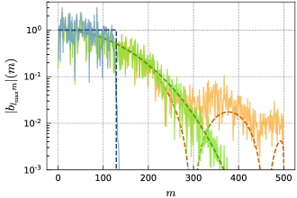
Figure 1: Effect of a primary beam on the $b_{\ell m}$. The norm of the beam modulated spherical harmonics coefficients of a simulated flat sky (solid line) is plotted for a fixed $\ell$ mode ($\ell=\ell_{\mathrm{max}}$) and compared against the profile of the primary beam $H(\mathrm{sin}^{-1}(\frac{m}{{\ell}}))$ (dashed line) for a top-hat (blue), Gaussian (green) and Bessel (orange) primary beam.

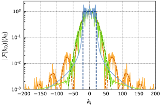
Figure 2: Effect of a primary beam on the $F_{\ell}[b_{\ell m}]$. The norm of $F_{\ell}[b_{\ell m}]$ of a simulated flat sky (solid line) is plotted for a fixed $m$ mode ($m=0$) and compared against the profile of the primary beam $H(\frac{2k_{\ell}}{\ell_{\mathrm{max}}-m}\pi)$ (dashed line) for a top-hat (blue), Gaussian (green) and Bessel (orange) primary beam.

which means that modulating the sky brightness by an axi-symmetric primary beam $H(\Omega_{k})$ is equivalent to modulating the associated Legendre functions. Exploring this relation, we find that multiplying the sky by a beam can be viewed as a convolution in $\ell$, and a multiplication in $m$. More specifically, for a fixed $\ell$, we have

$$b_{\ell m} \propto a_{\ell m}H(\mathrm{sin}^{-1}(\frac{m}{{\ell}})),$$ (24)

$$\mathcal{F_{\ell}}[b_{\ell m}](k_{\ell}) \propto \mathcal{F_{\ell}}[a_{\ell m}](k_{\ell})H(\frac{2\pi k_{\ell}}{\ell_{\mathrm{max}}-m}),$$ (25)

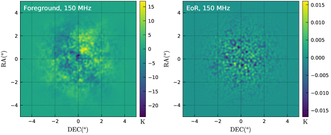
Figure 3: This figure shows a slice at 150 MHz for the diffuse foreground emission and the 21-cm eor signal template at a pixel resolution of 1.17 arc-min. Note that, the mean is subtracted from the maps. Each panel covers a region of $5^{\circ}\times 5^{\circ}$.

with $\mathcal{F_{\ell}}$ denoting the Fourier transform in $\ell$ (for a fixed $m$), $k_{\ell}$ the Fourier conjugate of $\ell$, $b_{\ell m}$ the spherical harmonics coefficient of the beam modulated sky, and $a_{\ell m}$ the spherical harmonics coefficient of the sky.

To experimentally confirm these relations, we simulate a Gaussian Random Field (GRF) on the sphere with a flat power spectra ($C_{\ell}=1$ for all $\ell$). This simulated sky is multiplied by a primary beam and we then compute the associated spherical harmonics coefficient using Eqn. 23. For this test, a top-hat, a Gaussian and a Bessel primary beam are used. In Fig.  1, the $b_{\ell m}$ (solid lines) are compared with the profile of the primary beam $H(\mathrm{sin}^{-1}(\frac{m}{{\ell}}))$ (dashed line), and in Fig. 2, the $\mathcal{F_{\ell}}[b_{\ell m}](k_{\ell})$ are compared with $H(\frac{2\pi k_{\ell}}{{\ell}-m})$. For the three beams, these experiments confirm that Eqn. 24 and Eqn. 25 are good approximation of the relation between the $b_{\ell m}$ and the primary beam profile $H(\theta_{k})$.

While we could not obtain an exact relation, these approximations are sufficient to define simple sampling rules. Reducing the sky Field of View (FoV) corresponds in the spherical-harmonics domain (defined at the phase-center) to reducing $m_{\mathrm{max}}(\ell)$, the maximum $m$ mode as function of $\ell$, and increasing $\Delta\ell$, the spacing between consecutive $\ell$ modes. Eqn. 25 suggests that these sampling rules are better applied in Fourier domain in $\ell$. Updating Eqn. 16 accordingly, we have,

$$\mathcal{V} = \textbf{{T}}\textbf{{F}}_{\ell}\textbf{{V}}_{\mathrm{ML}}+\textbf{{n}},$$ (26)

$$\textbf{{v}}_{\mathrm{ML}} = \textbf{{F}}_{\ell}^{-1}\textbf{{V}}_{\mathrm{ML}},$$ (27)

with F denoting the matrix form of the Fourier transform in $\ell$. We now solve for the $\textbf{{V}}_{\mathrm{ML}}$ using eqn. 26 and then compute the $\textbf{{v}}_{\mathrm{ML}}$ using eqn. 27. The size of $\textbf{{V}}_{\mathrm{ML}}$ can be reduced so that it contains only significant elements. Using Eqn.  24 and Eqn. 25, we can demonstrate that to fully describe the beam modulated sky up to $\theta_{\mathrm{max}}$, we can restrict the $k_{\ell}(m)$ modes of $\textbf{{V}}_{\mathrm{ML}}$ such that

$$|k_{\ell}(m)| <= \frac{\theta_{\mathrm{max}}(\ell_{\mathrm{max}}-m)}{2\pi},$$ (28)

$$m(l) <= \ell\,\mathrm{sin}(\theta_{\mathrm{max}}).$$ (29)

Using these sampling rules considerably reduce the computational scale of the problem. If we take for example a Gaussian primary beam with full width at half maximum (FWHM) $\theta_{\mathrm{fwmh}}$, it is reasonable to solve only for the ($\ell$, m) coefficients restricted to $\theta_{\mathrm{max}}\sim 2\theta_{\mathrm{fwmh}}$ without impacting the inversion strongly. For a FWHM of $4\degree$ and $\ell_{\mathrm{max}}=1570$, this reduce the number of coefficients to solve for from 1 185 351 to 7 864.

3 Full simulation

3.1 Simulated data templates

In this section we describe briefly the templates we considered for the EoR signal and diffuse foreground emission from which the visibility data were generated. In our formalism we assume that the bright extragalactic sources can be properly modeled and subtracted from the data, so they are not included in our foreground model.

3.1.1 EoR Signal

We have used the semi-analytic code 21cmFAST (Mesinger & Furlanetto, 2007; Mesinger et al., 2011) to simulate the EoR signal. 21cmFAST treats physical processes with approximate methods. Apart from the scales less than $<1{\rm Mpc}$, the output of this semi-analytic code tends to agree well with the hydro-dynamical simulations of Mesinger et al. (2011). The 21-cm EoR template used here is the same as used in Ghosh et al. (2015) and we refer the reader to Chapman et al. (2012) for details description of the simulations. The 21cmFAST simulation computes the $\delta T_{\mathrm{b}}$ box at each redshift based on the following equation,

$$\begin{split}\delta T_{\mathrm{b}}&=28\>\mathrm{mK}\times(1+\delta)x_{\mathrm{HI}}\left(1-\frac{T_{\mathrm{CMB}}}{T_{\mathrm{spin}}}\right)\left(\frac{\Omega_{b}h^{2}}{0.0223}\right)\\ &\qquad\times\sqrt{\left(\frac{1+z}{10}\right)\left(\frac{0.24}{\Omega_{m}}\right)},\end{split}$$ (30)

where, $\delta T_{\mathrm{b}}$ is the brightness temperature fluctuation which is detected as a difference from the background CMB temperature $T_{\mathrm{CMB}}$ (Field, 1958, 1959; Ciardi & Madau, 2003), $h$ is the Hubble constant in units of $100\>\mathrm{kms}^{-1}\>\mathrm{Mpc}^{-1}$, $x_{\mathrm{HI}}$ is the neutral hydrogen fraction and $\Omega_{b}$ and $\Omega_{m}$ are the baryon and matter densities in critical density units. We note that here we ignore the gradient of the peculiar velocity fluctuation whose contribution to the brightness temperature is relatively small (Ghara et al., 2015; Shimabukuro et al., 2015). We also assume that the neutral gas has been heated well above the CMB temperature during Epoch of Reionization ($T_{\mathrm{S}}\gg T_{\mathrm{CMB}}$) (Pritchard & Loeb, 2008) and therefore we can safely neglect the spin temperature fluctuations in generating the simulated 21-cm signal.

3.1.2 Diffuse foregrounds

The diffuse foreground model used in this paper include contribution from Galactic diffuse Synchrotron emission (GDSE), Galactic localized Synchrotron emission, Galactic diffuse free-free emission and unresolved extra-galactic foregrounds. We refer the reader to Jelić et al. (2008); Jelić et al. (2010) for a detail comprehensive review how the individual foreground components were simulated. Here, we highlight only few key features of the foreground simulations. Galactic diffuse Synchrotron emission (GDSE) originates due to the interaction of cosmic ray (CR) electrons produced mostly by supernova explosions and the Galactic magnetic field (Pacholczyk, 1970; Rybicki & Lightman, 1986). The intensity and the spectral index of the GDSE are modeled as Gaussian random fields (GRF) where the spatial power spectrum had a power law index of $-2.7$ and with frequency the GRF assumes a spectral index of $-2.55\pm 0.1$ (Shaver et al., 1999) with a fixed mean brightness temperature set around to $253\pm 1.3$ K at 120 MHz. The diffuse thermal (free-free) emission arises due to bremsstrahlung radiation in very diffuse ionized gas. At LOFAR-EoR frequencies the ionized gas is optically thin and the free-free emission from diffuse ionized gas is proportional to the emission measure. Here, the free-free emission is modeled as a GRF and spectral index is fixed to -2.15 (Tegmark et al., 2000; Santos et al., 2005) where the normalization is set with respect to the intensity of the $\rm{H}\alpha$ emission and fixed at $2.2$ K at 120 MHz (Smoot, 1998). The simulations of radio galaxies, used in this paper, are based on the extragalactic radio source counts at 151 MHz by Jackson (2005). Then the simulated radio galaxies are clustered using a random walk algorithm where the radio clusters are selected from the cluster catalogue of Virgo Consortium.

This diffuse foreground model is finally calibrated to have a spatial power spectra of 400 $\rm{mK}^{2}$ at 150 MHz and $\ell=400$, to match more closely with LOFAR (Patil et al., 2017) and Westerbork (Bernardi et al., 2010) observations of the diffuse emission on the NCP field.

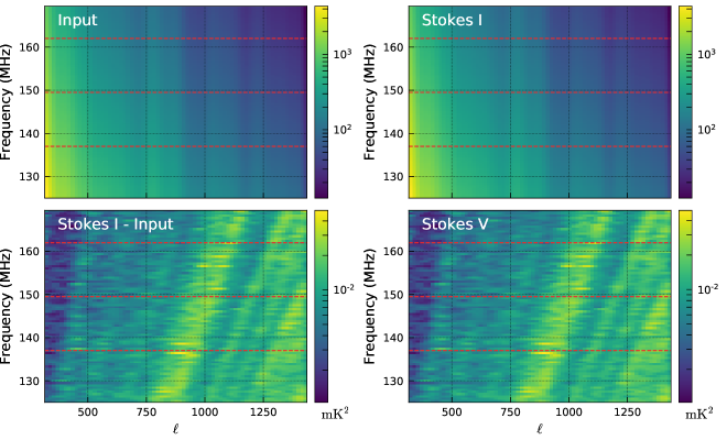
Figure 4: This figure shows the angular power spectrum as a function of angular scale $\ell$ and frequency $\nu$ for the input simulated sky composed of foregrounds diffuse emission and 21-cm signal (top-left panel), the Spherical-Harmonics(SpH) ML reconstructed Stokes I (top-right panel), the difference between the input sky and Stokes I (bottom-left) and SpH ML reconstructed Stokes V (bottom-right panel). The Stokes V power is due to the noise in the visibilities, and is similar to the difference in power between Stokes I and Input map. The red dashed line delimit the two frequency bins, 137.5-150 MHz ($z\sim 9$) and 150-162.5 MHz ($z\sim 8$) at which the three-dimensional power spectra are computed.

3.2 Simulating visibilities

The LOFAR-HBA antenna positions (van Haarlem et al., 2013) were used to generate the baseline components $(u,v,w)$ towards the North Celestial Pole (NCP) at which we predict visibilities corresponding to a combination of diffuse foregrounds and EoR only sky. Figure 3 shows a representative spatial slice at 150 MHz of the foreground and the EoR signal used in this simulation. We used a Gaussian primary beam with a FWHM of $4\degree$ (van Haarlem et al., 2013) to model the LOFAR primary beam which is multiplied with the input foreground and the 21-cm signal templates of $10\degree\times 10\degree$. The Cartesian maps were converted to spherical harmonics using the healpix package, and then transformed to visibilities using Eqn. 9. Next, we added random Gaussian noise to the real and imaginary part of the visibility separately where the rms of the noise were calculated from,

$$\sigma=\frac{\rm{SEFD}}{\sqrt{2\,\Delta\nu\,\Delta t}},$$ (31)

with $\Delta\nu$ and $\Delta t$ the frequency bandwidth and integration time, respectively. We assume that for LOFAR HBA the expected system equivalent flux density (SEFD) towards NCP is $\sim 4000$ Jy (van Haarlem et al., 2013). We note that the SEFD is generally elevation dependent and changes across the sky. We added Gaussian random noise with rms of 0.04 Jy, which corresponds to about 100 nights of 12 hours long LOFAR observation for a 0.5 MHz channel width and 100 s snapshot integration time. This integration time is chosen to reduce the number of visibilities and hence the complexity of the ML inversion, while avoiding time-smearing effect for the selected baseline range.

We simulate both visibilities including the sum of the foregrounds and the 21-cm signal input data template, which will be our Stokes I data set, and the visibilities of the noise only, which will be our Stokes V data set.

3.3 ML inversion and Power Spectra

From the simulated Stokes-I and Stokes-V visibilities, we infer the recovered spherical harmonics $b^{\mathrm{I}}_{\ell m}$ and $b^{\mathrm{V}}_{\ell m}$, using the maximum likelihood algorithm described in Sect. 2.3 and Sect. 2.4 and compute the angular power spectra via,

$$C_{\ell}=\frac{4\pi}{\Omega_{\mathrm{PB}}}\frac{1}{\ell+1}\sum_{m=0}^{\ell}|b_{\ell m}|^{2},$$ (32)

with $\Omega_{\mathrm{PB}}$ being the primary beam field of view (Parsons et al., 2012). Figure  4 shows the angular power spectra as function of $\ell$ and frequency for the input sky and for the recovered Stokes I and Stokes V. We find the input and the reconstructed angular power spectra for all the frequency channels resembles each other quite closely and this estimator can be used to jointly characterize the angular and frequency dependence of the observed sky signal. It also shows that the error introduced by the ML inversion is well below the thermal noise, as the power of the difference between the Stokes I and input sky is found to be similar to the Stokes V power. The diagonal structures observed in the Stokes V power spectra are related to baseline density. The noise is higher for $\ell$ modes corresponding to sparser baseline density which is a function of fixed baseline metric units and then scale to units of lambda as a function of frequency: $\ell=\frac{2\pi|\textbf{{b}}|}{\lambda}$ where b is the vector representing the coordinates in meters in the plane of the array.

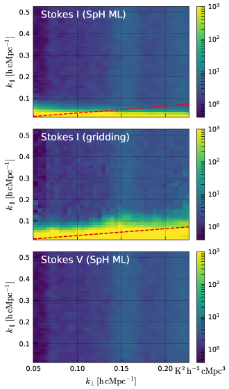
Figure 5: Cylindrically averaged power spectra estimated from the simulated visibilities. The top and middle panel shows the power spectra of the observed signal (foregrounds, noise and 21 cm signal; Stokes I) obtained from the spherical harmonics ML inversion (top) and by gridding the simulated visibilities using WSClean (middle). The absence of structure inside the 10 $\degree$ Field of View wedge line (red dashed line) in the power spectra estimated using the SpH ML inversion demonstrate that the method effectively compute PSF-deconvolved representation of the sky. The power spectra of the noise (Stokes V) is plotted in the bottom panel.

We then introduce the three-dimensional power spectra to quantify the entire second order statistics of the background sky signal by taking the Fourier transform of the $b_{\ell m}(\nu)$ cube in the frequency direction. We define the cylindrically averaged power spectra as (Parsons et al., 2012):

$$P(k_{\perp},k_{\parallel})=\frac{4\pi X^{2}Y}{\Omega_{\mathrm{PB}}B}\frac{1}{\ell+1}\sum_{m=0}^{\ell}\left|\hat{b}_{\ell m}(\eta)\right|^{2},$$ (33)

where $\eta$ is the Fourier conjugate of $\nu$, $\hat{b}_{\ell m}(\eta)$ the Fourier transform of the cube $b_{\ell m}(\nu)$, B the frequency bandwidth, X and Y are conversion factors from angle and frequency to comoving distance, and where the Fourier modes are in units of inverse comoving distance and are given by (Morales et al., 2006; Trott et al., 2012):

$$k_{\perp} =\frac{\ell}{D_{M}(z)},$$ (34)

$$k_{\parallel} =\frac{2\pi H_{0}f_{21}E(z)}{c(1+z)^{2}}\eta,$$ (35)

with $D_{M}(z)$ the transverse co-moving distance, $H_{0}$ the Hubble constant, $f_{21}$ the frequency of the hyperfine transition, and $E(z)$ the dimensionless Hubble parameter (Hogg, 1999).

It is important to point out that the three-dimensional power spectrum $P(k)$ is well suited to quantify the statistics of HI signal only if we perform it on limited frequency ranges which prevent the evolution of the HI signal across the line of sight, known as the Light-Cone effect (Datta et al., 2012), assuming the 21-cm signal to be statistically stationary in angular and frequency axis (Mondal et al., 2017; Ram Marthi et al., 2017). For this reason, we limit our estimation of the three dimensional power spectrum to frequency bands of 12.5 MHz. For the foregrounds, where the statistics are quite different for the chromatic response of the telescope the angular and frequency homogeneity assumption breaks down and the power spectrum $P(k)$ is no longer the obvious choice to quantify the statistical properties of the measured sky signal. For this latter case, the angular power spectrum estimator ($C_{\ell}$’s) as a function of frequency is more suitable. We note that this assumes homogeneity in angular domain but does not rely on the assumption of homogeneity in the frequency domain. We also note that when using the visibility correlation (Bharadwaj & Sethi, 2001; Bharadwaj & Ali, 2005; Ghosh et al., 2011; Ali et al., 2008; Ghosh et al., 2012), the angular power spectrum has been quantified earlier and the relation between the visibility correlations and the power spectrum $P({\bf{\rm k}})$ is also quite well known (Datta et al., 2007; Saiyad Ali & Bharadwaj, 2013).

3.3.1 Cylindrically averaged Power Spectra

Figure 5 presents the cylindrically averaged power spectra from the simulated visibilities using spherical harmonic ML inversion. We calculated the power spectrum for two cases. The top panel of figure 5 shows the power spectrum corresponding to diffuse foregrounds, 21-cm signal and noise (Stokes I), whereas the bottom panel displays the noise-only power spectrum (Stokes V). We calculate the power spectrum for a 12.5 MHz band around 150 MHz. We find the smooth diffuse foreground in the Stokes I power spectrum mostly dominates at low $k_{\parallel}$, where most of the foreground power is bound within $k_{\parallel}\leq 0.05\rm{hcMpc^{-1}}$. We find the power drops by two to three orders of magnitudes in high $k_{\parallel}$ regions, where the EoR plus noise signal is expected to dominate. On the other hand, the Stokes V power spectrum is more uniform and increases at higher $k_{\perp}$ scales where the baseline density of LOFAR drops with respect to the central core region.

The mode-mixing introduced by the instrument chromaticity are usually confined to a wedge-like structure in k space (Datta et al., 2010; Morales et al., 2012). This wedge line is defined by:

$$k_{\parallel}=\left[\mathrm{sin}(\theta_{\mathrm{field}})\frac{H_{0}D_{M}(z)E(z)}{c(1+z)}\right]k_{\perp},$$ (36)

where $\theta_{\mathrm{field}}$ is the angular radius of the FoV. In the power spectra obtained from the same simulated visibilities but using the more traditional method of gridding the visibilities in uv-space, a wedge like structure is clearly visible (middle panel of Figure 5), and is well known to be due to the frequency dependence of the PSF (Vedantham et al., 2012; Hazelton et al., 2013). Because our method consists of doing a ML fit to non-gridded visibility data sets at each frequency, we effectively obtain a PSF-deconvolved estimates of the sky spherical harmonics coefficients. The mode-mixing due to the PSF frequency dependence is then considerably reduced, demonstrated by the absence of a wedge in our ML power spectra estimates (top panel of Figure 5).

3.3.2 Spherically averaged Power Spectra

Next, we averaged the power spectrum in spherical shells and computed the spherically averaged dimensionless power spectrum, $\Delta^{2}({\bf{\rm k}})={\rm k^{3}P}({\bf{\rm k}})/2\pi^{2}$. In Fig. 6 we present the power spectrum in units of $\mathrm{mK}^{2}$ corresponding to Stokes I and Stokes V visibilities. We observe that the spherically averaged power spectrum for the Stokes I signal is mostly flat in the k range sampled by our simulation, whereas the Stokes V or the noise power spectrum rises steeply from the low k to high k values. It is also noteworthy that both the Stokes I and Stokes V spherically averaged power spectra are at-least order of magnitude higher compared to the 21cm signal and hence the signal to noise (S/N ratio) is always low in our simulation. In Fig. 6 we compare our power spectrum estimates using both the spherical harmonic ML inversion (solid line) and Cartesian ML inversion techniques (dashed line) as introduced in Ghosh et al. (2015) which we briefly expose here. Ideally, the simulated visibility records a single mode of the Fourier transform of the specific intensity distribution $I_{\nu}(\ell,m)$ corresponding to the simulated sky. Representing the celestial sphere by a unit sphere, the component $n$ can be expressed in terms of $(l,m)$ by $n(l,m)=\sqrt{1-l^{2}-m^{2}}$. Then the measured visibility for monochromatic, unpolarized signal is,

$$\begin{split}\mathcal{V}_{\nu}(u,v,w)&=\int\frac{I_{\nu}(l,m)}{\sqrt{1-l^{2}-m^{2}}}\\ &\qquad\times e^{-2\pi i(ul+vm+w(\sqrt{1-l^{2}-m^{2}}-1))}\mathrm{d}l\mathrm{d}m.\end{split}$$ (37)

We recall that Eqn. 37 can be re-written in vector form (similar to Eqn. 16), where we used the Fourier kernel, $e^{-2\pi i(ul+vm+w(\sqrt{1-l^{2}-m^{2}}-1))}$, is the response matrix T and $\frac{I_{\nu}(l,m)}{\sqrt{1-l^{2}-m^{2}}}\times d\Omega_{p}$ is the model sky parameters that we want to directly infer from the visibility data. It is interesting to point out that without any loss of generality (assuming that all stations have identical primary beams) we can incorporate the Primary Beam (PB) pattern in the response matrix (Ghosh et al., 2015) and close to the phase center the inverted specific intensity distribution closely follows to that where no primary beam pattern is introduced. Hence, we decided not to introduce any PB in the visibilities corresponding to the Cartesian ML solutions.

We notice that both Cartesian and Spherical-Harmonics ML inversion estimates are quite close to each other across the whole k range sampled by our simulation. This is also expected as we have restricted ourselves to a $\sim 4\degree$ window (which corresponds to the full width half maxima ($\theta_{\mathrm{fwhm}}$) LOFAR-HBA stations) from the phase center where the effects due to sky curvature is minimal. We also compared the difference between the input and the reconstructed power spectrum from the spherical harmonic and Cartesian ML inversion techniques. We note that the Cartesian ML approach assumes a finite field for the sky model and hence does not account for structure outside the FoV , hence leaves residual side-lobe noise. This is more apparent for large angular scales where the Cartesian ML inversion error increases compared to the SpH analysis, being the more appropriate choice for large scales. We find that the difference between the input and the spherical harmonic estimates (solid orange) is lower than difference between the input and the Cartesian ML estimates (dashed orange line). For both redshifts z=8 and z=9, the error due to the reconstruction lies well below the fiducial 21-cm signal, which is shown in gray in Figure 6. This is an important point as it shows that the error introduce by our SpH estimator will not affect the statistical detection of the EoR signal across the whole k range probed by the current simulation. Also, the SpH method could be further improved by increasing the number of ($\ell,m$) modes beyond that currently set by our sampling rule.

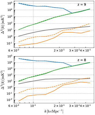
Figure 6: Spherically averaged power spectra of Stokes I (blue) and Stokes V (green). The power spectra estimated using the spherical harmonics ML inversion (solid line) is compared to the power spectra estimated using the Cartesian ML inversion (dashed line). The difference between the input power spectra and estimated power spectra (orange) is lowered using the spherical harmonics ML inversion, and is well below the 21 cm signal power spectra (gray).

4 Foreground removal algorithms

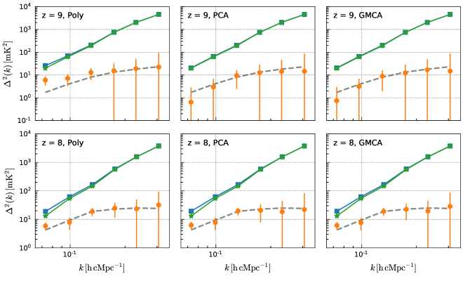
Figure 7: Detection of the 21-cm signal using the spherically averaged power spectra. Subtracting the noise bias (green) from Stokes I residual power spectra after the foreground removal step (blue), we can recover the power spectra of the 21-cm line signal (orange) which is compared to the input 21-cm signal (gray dashed line). The error bar corresponds to 2-$\sigma$ sampling variance.

Though the astrophysical foregrounds are expected to be approximately three to four orders of magnitudes larger than the cosmological 21-cm HI signal, the two signals have a markedly different frequency structure. The HI signal is expected to be uncorrelated on frequency scales on the order of MHz, where as the foregrounds are expected to be smooth in frequency. In this paper we have implemented different foreground modeling techniques where for each ($\ell$, m) mode we model the foreground as a smooth component in frequency. In the following subsections, we briefly describe our foreground removal techniques.

4.1 Polynomial Fitting

Probably, the most intuitively simplest method for foreground removal is to choose an ad-hoc basis of smooth functions such as polynomial fitting in frequency or log-frequency that we think can describe the foregrounds (McQuinn et al., 2006; Morales et al., 2006; Jelić et al., 2008; Bowman et al., 2006; Liu et al., 2009). Here, we use polynomial fitting to fit each individual ($\ell$, m) mode along the line of sight direction. When fitting in log space, we offset the data to avoid negative values. In log-log space our polynomial model is as follows:

$$\mathrm{log}(b_{\ell m}(\nu))=\sum_{k=0}^{N_{\mathrm{fg}}}\alpha_{\ell m}^{k}[\mathrm{log}(\nu)]^{k},$$ (38)

where, $N_{\mathrm{fg}}$ is the order of the polynomial and $\alpha_{\ell m}^{k}$ are the coefficients of the polynomials.

One needs to carefully choose the order of the polynomial to avoid over or under-fitting the foreground which could negatively affect the 21-cm EoR signal. Although, the polynomial order can be chosen in a Bayesian manner where we can choose the particular polynomial model which has the highest evidence based on the data we have. In this paper, we choose to fit 2nd order polynomial for each ($\ell,m$) modes whereas with both lower and higher order fits we find a worse result.

4.2 Principal Component Analysis (PCA)

Principal component analysis (PCA) utilizes the main properties of the foregrounds such as their large amplitude and smooth frequency coherence to find the largest foreground components and an optimal set of basis functions at the same time (Harker et al., 2009; Masui et al., 2013; Switzer et al., 2013; Alonso et al., 2015). As the foreground are highly correlated in frequency the frequency- frequency co-variance matrix of the continuum foregrounds will have a particular eigen system where most of the information can be sufficiently described by a small set of very large eigenvalues, the other ones being negligibly small. Thus, we can attempt to subtract the foregrounds by eliminating from the recovered ($\ell$, m) modes the components corresponding to the eigen-vectors of the frequency co-variance matrix with the largest associated eigenvalues. In this paper, we choose to remove 2 PCA components for each ($\ell$, m) mode which captured most of the variance of the foreground modes. This number will essentially depend on the frequency structure of the foregrounds and the different instrumental effects.

4.3 Generalized Morphological Component Analysis (GMCA)

GMCA is a blind source separation technique (BSS) (Bobin et al., 2008) which assumes that a wavelet basis exists in which the smooth continuum foregrounds can be sparsely represented with a few basis coefficients and thus can be separated from EoR signal and noise (Chapman et al., 2013). It is labeled as a non-parametric method due to the lack of parameterized model for foregrounds which are largely unknown at the low frequencies of interest. It uses the data to decide on the foreground model. We note that GMCA is able to clean the foregrounds based on both in spatial and frequency direction information contained within the foreground signal compared to the cosmological signal and instrumental noise. The result leads to a very different basis coefficients for the foregrounds and the residual signal which is a combination of the method and the instrumental noise.

4.4 Application to the simulation

In our simulation setup, we tried only to remove a minimal number of foreground degrees of freedom (for example in case of the PCA method we look for the first two modes corresponding to the highest variance) and thereby minimizing the risk of subtracting the 21-cm EoR signal. We also assume that we know the noise variance across the different k scales from Stokes V so that we can subtract the noise power spectrum from the data and compare the residuals with the input 21-cm EoR power spectrum. In Figure 7 we show the recovered Stokes I power spectrum from the SpH ML method, the Stokes V (noise power spectrum), the residual (Stokes I - Stokes V) and the power spectrum corresponding to the 21-cm EoR signal. We find, all the foreground removal methods recover the input power spectrum quite well for $k\leq 0.1\rm{h\,cMpc^{-1}}$.

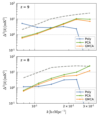
Figure 8: Spherically averaged power spectra of the foregrounds fitting error for the three different techniques used: the log-polynomial method (blue), the PCA method (green) and the GMCA method (red). The foregrounds fitting error is found to be below the 21-cm input signal (gray dashed line) in most situation except when using log-polynomial method at $z=9$.

We observe that we can recover the input foreground model fairly well using all three methods and that the differences between the input and recovered foreground model are well below the fiducial 21-cm EoR signal at redshift z=8, whereas we notice that at redshift z=9 the error is comparable to the EoR signal below $k\leq 0.1\rm{h\,cMpc^{-1}}$, but lies well below the EoR signal for higher $k$ ranges (Fig. 8). We also note all the three foreground-removal approaches show similar extent of errors in reconstructing the input foreground models, although at lower $k$ scales ($k\leq 0.1\rm{h\,cMpc^{-1}}$) PCA and GMCA seem to work better than the polynomial fitting method. We note this is mainly due to the differences in the three FG removal methods and our SpH ML inversion method works perfectly well in reconstructing the input signal across all the $k$ values probed by our current simulations (Fig. 6).

5 Conclusions

In this paper we have introduced a maximum likelihood spherical wave function harmonic decomposition of the complex visibilities. The method can produce wide- field images which will be a key component for next generation interferometers with large field of view and new wide-field imaging challenges (ionosphere, beam modeling etc.). The method has been formulated in a full sky setting including the primary beam and its side-lobes, allowing us to model large parts of the sky (up to a chosen $\theta_{\mathrm{max}}$) by considerably reducing the far side- lobe noise which is an addition noise component due to the un-modeled structure in the sky. We have shown, based on a spherical wave-function ML fit in the visibility domain, that it is possible to deconvolve the chromatic “wedge" (caused by frequency-dependent side-lobes) in the ($\rm{k}_{\perp},\rm{k}_{\parallel}$) power spectrum space, thus leaving us with a relatively wider ‘clean’ window to isolate the faint 21-cm EoR signal compared to the order of magnitude strong foregrounds. This is particularly important when aiming to achieve the expected level of sensitivity of future instruments such as the SKA, for which it is expected that the far-out side-lobes of the station beam will have a substantial impact on high dynamic range image performance (Cornwell & Perley, 1992; McEwen & Scaife, 2008; Carozzi & Woan, 2009; Carozzi, 2015).

We have shown that the coefficient of the visibility distribution in spherical coordinates is linearly related with the sky brightness distribution over a celestial sphere. Hence, by decomposing the visibilities in spherical wave functions, one provides a reconstruction of the sky brightness distribution without any extra computational cost. To reduce the computational load, we have introduced a sampling scheme which speeds up the inversion considerably. In a LOFAR-HBA full-sky simulation, including the 21-cm EoR signal, diffuse foregrounds and a Gaussian random noise with rms of 0.04 Jy roughly corresponding to 100 nights of 12 hr LOFAR integration time, we find that we can recover the input power spectrum quite well across the whole $k$ range $0.07-0.3\,\rm{h\,cMpc^{-1}}$. The foreground cleaning techniques implemented in our current scheme works reasonably well and we notice that we can recover the input EoR power spectrum assuming the noise power spectrum is known accurately.

Finally, we note that the simulated foregrounds and instrument model used in this paper is not complete and does not include other foregrounds contaminants such as the instrumental polarization leakage, the frequency dependence of the individual LOFAR HBA station’s primary beam and the phase errors caused by the ionosphere or imperfect calibration. To tackle this problem, we are currently working on a new foreground removal algorithm able to model multiple arbitrarily non-smooth foreground contaminants, along with estimating their statistical error, considerably improving the foregrounds model at the lowest $k$ where the 21-cm EoR signal also peaks, and delivering the full potential of the instrument.

The code implementing the algorithm described in this paper is freely available at https://gitlab.com/flomertens/sph_img.

References

- Ali et al. (2008) Ali S. S., Bharadwaj S., Chengalur J. N., 2008, MNRAS, 385, 2166
- Alonso et al. (2015) Alonso D., Bull P., Ferreira P. G., Santos M. G., 2015, MNRAS, 447, 400
- Bernardi et al. (2010) Bernardi G., et al., 2010, A&A, 522, A67
- Bharadwaj & Ali (2005) Bharadwaj S., Ali S. S., 2005, MNRAS, 356, 1519
- Bharadwaj & Sethi (2001) Bharadwaj S., Sethi S. K., 2001, Journal of Astrophysics and Astronomy, 22, 293
- Bhatnagar et al. (2013) Bhatnagar S., Rau U., Golap K., 2013, ApJ, 770, 91
- Bobin et al. (2008) Bobin J., Moudden Y., Starck J.-L., Fadili J., Aghanim N., 2008, Statistical Methodology, 5, 307
- Bolton et al. (2011) Bolton J. S., Haehnelt M. G., Warren S. J., Hewett P. C., Mortlock D. J., Venemans B. P., McMahon R. G., Simpson C., 2011, MNRAS, 416, L70
- Bosman & Becker (2015) Bosman S. E. I., Becker G. D., 2015, MNRAS, 452, 1105
- Bouwens et al. (2010) Bouwens R. J., et al., 2010, ApJ, 709, L133
- Bowman et al. (2006) Bowman J. D., Morales M. F., Hewitt J. N., 2006, ApJ, 638, 20
- Carozzi (2015) Carozzi T. D., 2015, MNRAS, 451, L6
- Carozzi & Woan (2009) Carozzi T. D., Woan G., 2009, MNRAS, 395, 1558
- Chapman et al. (2012) Chapman E., et al., 2012, MNRAS, 423, 2518
- Chapman et al. (2013) Chapman E., et al., 2013, MNRAS, 429, 165
- Choudhuri et al. (2014) Choudhuri S., Bharadwaj S., Ghosh A., Ali S. S., 2014, MNRAS, 445, 4351
- Ciardi & Madau (2003) Ciardi B., Madau P., 2003, ApJ, 596, 1
- Cornwell & Perley (1992) Cornwell T. J., Perley R. A., 1992, A&A, 261, 353
- Cornwell et al. (2005) Cornwell T. J., Golap K., Bhatnagar S., 2005, in Kassim N., Perez M., Junor W., Henning P., eds, Astronomical Society of the Pacific Conference Series Vol. 345, From Clark Lake to the Long Wavelength Array: Bill Erickson’s Radio Science. p. 350
- Datta et al. (2007) Datta K. K., Choudhury T. R., Bharadwaj S., 2007, MNRAS, 378, 119
- Datta et al. (2010) Datta A., Bowman J. D., Carilli C. L., 2010, ApJ, 724, 526
- Datta et al. (2012) Datta K. K., Mellema G., Mao Y., Iliev I. T., Shapiro P. R., Ahn K., 2012, MNRAS, 424, 1877
- Di Matteo et al. (2002) Di Matteo T., Perna R., Abel T., Rees M. J., 2002, ApJ, 564, 576
- Dillon et al. (2015) Dillon J. S., et al., 2015, Phys. Rev. D, 91, 123011
- Fan et al. (2006) Fan X., Carilli C. L., Keating B., 2006, ARA&A, 44, 415
- Field (1958) Field G. B., 1958, Proceedings of the IRE, 46, 240
- Field (1959) Field G. B., 1959, ApJ, 129, 536
- Furlanetto et al. (2006) Furlanetto S. R., Oh S. P., Briggs F. H., 2006, Phys. Rep., 433, 181
- Ghara et al. (2015) Ghara R., Choudhury T. R., Datta K. K., 2015, MNRAS, 447, 1806
- Ghosh et al. (2011) Ghosh A., Bharadwaj S., Ali S. S., Chengalur J. N., 2011, MNRAS, 418, 2584
- Ghosh et al. (2012) Ghosh A., Prasad J., Bharadwaj S., Ali S. S., Chengalur J. N., 2012, MNRAS, 426, 3295
- Ghosh et al. (2015) Ghosh A., Koopmans L. V. E., Chapman E., Jelić V., 2015, MNRAS, 452, 1587
- Harker et al. (2009) Harker G., et al., 2009, MNRAS, 397, 1138
- Hazelton et al. (2013) Hazelton B. J., Morales M. F., Sullivan I. S., 2013, ApJ, 770, 156
- Hogg (1999) Hogg D. W., 1999, ArXiv Astrophysics e-prints,
- Jackson (2005) Jackson C., 2005, Publ. Astron. Soc. Australia, 22, 36
- Jelić et al. (2008) Jelić V., et al., 2008, MNRAS, 389, 1319
- Jelić et al. (2010) Jelić V., Zaroubi S., Labropoulos P., Bernardi G., de Bruyn A. G., Koopmans L. V. E., 2010, MNRAS, 409, 1647
- Kim (2007) Kim J., 2007, MNRAS, 375, 625
- Liu et al. (2009) Liu A., Tegmark M., Bowman J., Hewitt J., Zaldarriaga M., 2009, MNRAS, 398, 401
- Liu et al. (2016) Liu A., Zhang Y., Parsons A. R., 2016, ApJ, 833, 242
- Masui et al. (2013) Masui K. W., et al., 2013, ApJ, 763, L20
- McEwen & Scaife (2008) McEwen J. D., Scaife A. M. M., 2008, MNRAS, 389, 1163
- McQuinn et al. (2006) McQuinn M., Zahn O., Zaldarriaga M., Hernquist L., Furlanetto S. R., 2006, ApJ, 653, 815
- Mellema et al. (2013) Mellema G., et al., 2013, Experimental Astronomy, 36, 235
- Mesinger (2010) Mesinger A., 2010, MNRAS, 407, 1328
- Mesinger & Furlanetto (2007) Mesinger A., Furlanetto S., 2007, ApJ, 669, 663
- Mesinger et al. (2011) Mesinger A., Furlanetto S., Cen R., 2011, MNRAS, 411, 955
- Mondal et al. (2017) Mondal R., Bharadwaj S., Datta K. K., 2017, preprint, (arXiv:1706.09449)
- Morales & Wyithe (2010) Morales M. F., Wyithe J. S. B., 2010, ARA&A, 48, 127
- Morales et al. (2006) Morales M. F., Bowman J. D., Hewitt J. N., 2006, ApJ, 648, 767
- Morales et al. (2012) Morales M. F., Hazelton B., Sullivan I., Beardsley A., 2012, ApJ, 752, 137
- Oesch et al. (2013) Oesch P. A., et al., 2013, ApJ, 773, 75
- Oh & Mack (2003) Oh S. P., Mack K. J., 2003, MNRAS, 346, 871
- Pacholczyk (1970) Pacholczyk A. G., 1970, Radio astrophysics. Nonthermal processes in galactic and extragalactic sources
- Parsons et al. (2012) Parsons A. R., Pober J. C., Aguirre J. E., Carilli C. L., Jacobs D. C., Moore D. F., 2012, ApJ, 756, 165
- Patil et al. (2017) Patil A. H., et al., 2017, ApJ, 838, 65
- Planck Collaboration et al. (2014) Planck Collaboration et al., 2014, A&A, 571, A16
- Pober et al. (2013) Pober J. C., et al., 2013, ApJ, 768, L36
- Pritchard & Loeb (2008) Pritchard J. R., Loeb A., 2008, Phys. Rev. D, 78, 103511
- Ram Marthi et al. (2017) Ram Marthi V., Chatterjee S., Chengalur J., Bharadwaj S., 2017, preprint, (arXiv:1707.05335)
- Rau et al. (2009) Rau U., Bhatnagar S., Voronkov M. A., Cornwell T. J., 2009, IEEE Proceedings, 97, 1472
- Robertson et al. (2013) Robertson B. E., et al., 2013, ApJ, 768, 71
- Robertson et al. (2015) Robertson B. E., Ellis R. S., Furlanetto S. R., Dunlop J. S., 2015, ApJ, 802, L19
- Rybicki & Lightman (1986) Rybicki G. B., Lightman A. P., 1986, Radiative Processes in Astrophysics
- Saiyad Ali & Bharadwaj (2013) Saiyad Ali S., Bharadwaj S., 2013, preprint, (arXiv:1310.1707)
- Santos et al. (2005) Santos M. G., Cooray A., Knox L., 2005, ApJ, 625, 575
- Schenker et al. (2013) Schenker M. A., et al., 2013, ApJ, 768, 196
- Shaver et al. (1999) Shaver P. A., Windhorst R. A., Madau P., de Bruyn A. G., 1999, A&A, 345, 380
- Shaw et al. (2014) Shaw J. R., Sigurdson K., Pen U.-L., Stebbins A., Sitwell M., 2014, ApJ, 781, 57
- Shimabukuro et al. (2015) Shimabukuro H., Yoshiura S., Takahashi K., Yokoyama S., Ichiki K., 2015, MNRAS, 451, 467
- Smoot (1998) Smoot G. F., 1998, ArXiv Astrophysics e-prints,
- Switzer et al. (2013) Switzer E. R., et al., 2013, MNRAS, 434, L46
- Tegmark (1997) Tegmark M., 1997, ApJ, 480, L87
- Tegmark et al. (2000) Tegmark M., Eisenstein D. J., Hu W., de Oliveira-Costa A., 2000, ApJ, 530, 133
- Thompson et al. (2001) Thompson A. R., Moran J. M., Swenson Jr. G. W., 2001, Interferometry and Synthesis in Radio Astronomy, 2nd Edition
- Treu et al. (2013) Treu T., Schmidt K. B., Trenti M., Bradley L. D., Stiavelli M., 2013, ApJ, 775, L29
- Trott et al. (2012) Trott C. M., Wayth R. B., Tingay S. J., 2012, ApJ, 757, 101
- Vedantham et al. (2012) Vedantham H., Udaya Shankar N., Subrahmanyan R., 2012, ApJ, 745, 176
- Wyithe & Loeb (2004) Wyithe J. S. B., Loeb A., 2004, Nature, 432, 194
- Zheng et al. (2017) Zheng H., et al., 2017, MNRAS, 465, 2901
- van Haarlem et al. (2013) van Haarlem M. P., et al., 2013, A&A, 556, A2